Some new results for the GHWS model

Abstract

Here we outline some new results for the GHWS model which points to a discretization of parameter space into well differentiated collective dynamic states. We argue this can lead to basic processes in parameter space, starting with minimum modelling ingredients: a complex network with a disorder parameter and an excitable dynamics (cellular automata) on it.

‘dynamics first and consolidation to symbols later’

In reference [1] numerical results for the GHWS model were presented. One of the main results was that we can change the collective state of the system by changing network disorder alone, at constant coupling $\sigma=rK$, where $K$ is the average coordination number in the WS network and $r$ is the transmission coefficient in the GH automaton. We reproduce equation $(2)$ from reference [1] here:

$$\sigma_{c}=\Delta_{\sigma}\exp[-(x/\tau)^{\beta}]+\sigma_{c1}$$ (1)

which summarizes numerical results for the frontier between extinct and active collective states. That frontier in [1] was obtained by considering as extinct states those for which, after $T$ steps, the activity was zero ($F=0$) for all $M$ generated samples which differ in their random initial condition and rewiring. Equation (1) is a stretched exponential (with exponent $\beta$) in the rewiring odd $x=p/(1-p)$, where $p$ is the rewiring probability in the WS network.

Further numerical results for the activity $F(z,\sigma)$ in parameter space can be seen in figure 1, with disorder $z=\log[p/(1-p)]$ and with the absorbing state depicted in black. We have confirmed that the following simplification to eq. (1) holds:

$$\sigma_{c}=\Delta_{\sigma}\left(1+\exp[-(x/\tau)^{\beta}]\right)$$ (2)

that is: $\sigma_{c1}\approx\Delta_{\sigma}$, with $\Delta_{\sigma}\approx 1.2$ from our numerical experiments, for some $K$ and $N$ (see below).

Even more relevant than $F$ for a possible connection with experiments should be the (normalized) fluctuations of activity $\varsigma$ [2]:

$$\varsigma=\frac{N}{\langle F\rangle(1-\langle F\rangle)}\left[\langle F^{2}\rangle-\langle F\rangle^{2}\right]$$ (3)

with $\varsigma\approx 1$ implying a near ideal gas like dynamics (no correlations of activity) [2]. $\varsigma(z,\sigma)$ can be appreciated in figures 2 and 3 for some values of $K$ and $N$, where $N$ is the number of nodes in the network. For $K=6$ and $N=1000$ we can see the further relevance of the quantity $\Delta_{\sigma}$, where the curve $\varsigma=1$ is obtained by displacing the extinct-active frontier as $\sigma\rightarrow\sigma+\Delta_{\sigma}$ in the whole range of disorder $z$. The curve $\varsigma=1$ (for $K=6$) in parameter space in fact provides a better method for measuring $\Delta_{\sigma}$, which can be used to locate back the extinct-active frontier.

Thus, the quantity $\Delta_{\sigma}$ is not only a disorder-dependent activation threshold, but provides further structure in parameter space in connection with a dynamic state for which we have a clear interpretation ($\varsigma=1$).

We can see from figures 1, 2 and 3 that we can talk about of two phases in the GHWS model, for which $\partial\varsigma/\partial z=0$ (and $\partial F/\partial z=0$): an ordered phase (say $z<-10$) and a disordered phase (say $z>4$). Fluctuations and patterns of activity for both phases can be seen in figures 4 and 5. Note the different way in which large correlations of activity manifest themselves in the ordered and disordered phases near the extinct-active frontier (fluctuations $\Leftrightarrow$ correlations [2]).

Thus, at least for $K=6$, we obtain characteristic and differentiated dynamic states for couplings $\sigma$ near:

$$\sigma_{ms}=\Delta_{\sigma}(1+s+m)$$ (4)

where $s=0,1$ and $m=0,1,2,3,\ldots$ are integer numbers. For the ordered phase $s=1$, and $s=0$ for the disordered phase. For $(m,s)=(0,0)$ we get a dynamic state near the extinct-active frontier in the disordered phase. For $(m,s)=(0,1)$ we get a dynamic state near the extinct-active frontier in the ordered phase. For $(m,s)=(1,0)$ and $(m,s)=(1,1)$ we obtain a state with $\varsigma=1$. If $\varsigma<1$ ($m>1$) then we have negative average correlations of activity, and we have states with random-like patterns of activity, with high values of activity (see figure 1), and with a peak in the power spectra of activity at frequency $1/3$ (at least for small $K$): the microscopic natural frequency for each neuron with three states surfaces to macroscopic activity, see figure 6. That microscopic natural frequency equal to $1/3$ is certainly the case in the deterministic limit $r\rightarrow 1$.

By looking at figures 2 and 3 it seems that how good is equation (4) for describing our numerical results is a function of average coordination number $K$ and number of nodes $N$. Around $K=6$ and $N=1000$ it appears to be a good approximation. Thus, for certain $K$ and $N$, we obtain a natural discretization of parameter space, a consolidation to symbols [3], see figure 7. It would be natural now to consider processes in parameter space, between these reference system’s states labeled by integer numbers $(m,s)$.

From a mean field approximation we can obtain $\sigma_{c}=1$. It is natural then to write $\Delta_{\sigma}=1+\triangleright$, with the quantity $\triangleright$ associated to correlations of activity. We could rewrite equation (4) as

$$\sigma_{ms}=(1+\triangleright)(1+s+m)$$ (5)

It should be expected some relationship between $\triangleright$ and $\varsigma$, and may be that connection could be found in the behaviour of $\varsigma(\sigma)$ around $\varsigma=1$ for the ordered and disordered phases, see figure 4.

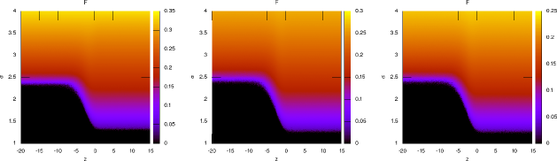
Figure 1: Activity $F(z,\sigma)$ for $K=4$ (left), $K=6$ (center), $K=8$ (right). $N=1000$. In this figure and also on figures 2 and 3 we plot $1000\times 1000$ points in parameter space $(z,\sigma)$, each of them obtained from a single run. We depict in black the absorbing state.

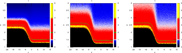
Figure 2: Normalized fluctuations of activity $\varsigma(z,\sigma)$ for $K=4$ (left), $K=6$ (center), $K=8$ (right). Note in green the reference value $\varsigma=2$, which is close to the extinct-active boundary in parameter space. After a transient of $T=1000$ time steps we considered the next $1000$ steps for obtaining the fluctuations. $N=1000$.

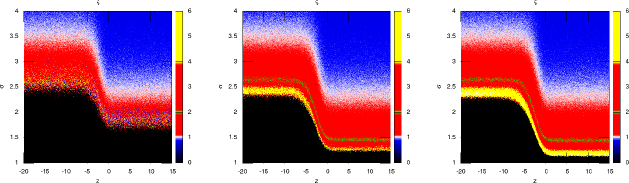
Figure 3: Normalized fluctuations of activity $\varsigma(z,\sigma)$ for $K=6$ with $N=100$ (left), $N=1000$ (center), $N=10000$ (right). Note in green the reference value $\varsigma=2$, which is close to the extinct-active boundary in parameter space.

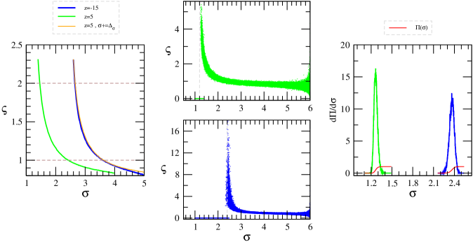
Figure 4: Normalized fluctuations of activity $\varsigma$ for ordered and disordered phases ($K=6$, $N=1000$). Note on the left the overlapping of $\varsigma(\sigma)$ for ordered and disordered phases once displaced by $\Delta_{\sigma}=1.2$ (for $\varsigma\in(0.9,2.3)$). Also, on the right, we show the variation of the fraction of active samples after $T=1000$ time steps $\Pi$ with respect to the coupling parameter $\sigma$ as a function of $\sigma$. At left and right we show averages over $M=1000$ samples. At center we show results from single runs.

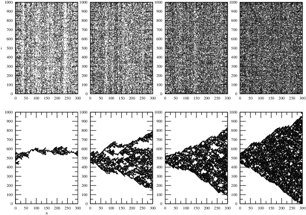
Figure 5: Patterns of activity. From right to left we get closer to the extinct-active frontier. top: disordered phase ($\sigma=1.3,1.4,1.5,1.6$). bottom: ordered phase ($\sigma=2.4,2.6,2.8,3.0$). ($K=6$, $N=1000$). For these eight plots: random initial conditions only on $100$ nodes in the center of the array, the rest in the susceptible state.

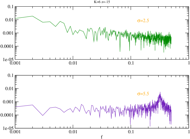
Figure 6: Power spectra of activity, from a single run, for the ordered phase, with $\sigma=2.5$ and $\sigma=5.5$. $K=6$ and $N=1000$.

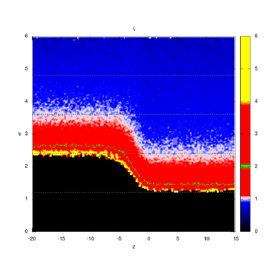
Figure 7: Discretization of parameter space for $K=6$ and $N=1000$. We show $200\times 200$ points. In dashed lines we show $\sigma=a\Delta_{\sigma}$, with $a=1,2,3,4$ and $\Delta_{\sigma}=1.2$.

References

- [1] Reyes L, Laroze D., Cellular Automata for excitable media on a Complex Network: The effect of network disorder in the collective dynamics, Physica A 588, 126552 (2022).
- [2] Chandler D., Introduction To Modern Statistical Mechanics, Oxford University Press, 1987. See section .
- [3] Kunihiko Kaneko, Life: An Introduction to Complex Systems Biology, Springer-Verlag Berlin Heidelberg, 2006.