Joint or Disjoint: Mixing Training Regimes for Early-Exit Models

Abstract

Early exits are an important efficiency mechanism integrated into deep neural networks that allows for the termination of the network’s forward pass before processing through all its layers. By allowing early halting of the inference process for less complex inputs that reached high confidence, early exits significantly reduce the amount of computation required. Early exit methods add trainable internal classifiers which leads to more intricacy in the training process. However, there is no consistent verification of the approaches of training of early exit methods, and no unified scheme of training such models. Most early exit methods employ a training strategy that either simultaneously trains the backbone network and the exit heads or trains the exit heads separately. We propose a training approach where the backbone is initially trained on its own, followed by a phase where both the backbone and the exit heads are trained together. Thus, we advocate for organizing early-exit training strategies into three distinct categories, and then validate them for their performance and efficiency. In this benchmark, we perform both theoretical and empirical analysis of early-exit training regimes. We study the methods in terms of information flow, loss landscape and numerical rank of activations and gauge the suitability of regimes for various architectures and datasets.

1 Introduction

Deep neural networks have achieved remarkable results across a variety of machine learning tasks. While the depth of these networks significantly contributes to their enhanced performance, the necessity of using large models for all inputs, especially in resource-constrained environments like mobile and edge computing devices, is questionable.

Early-exit methods in deep neural networks (DNNs) have gained importance due to their potential to significantly improve computational efficiency. By enabling exits at earlier layers, these methods can decrease the number of operations needed, leading to faster inference times. Early-exit methods allow the network to adapt its complexity based on the input. Simpler inputs can be processed with fewer layers, while more complex inputs can utilize the network’s full capacity.

Early exit methods are implemented through modification of the original architecture by adding internal classifiers (ICs) at selected layers. These ICs are designed to perform classification tasks based on the representations available at their respective positions in the network.

A common approach for training early-exit models involves training the entire network, both the original and added internal classifiers, from scratch [3, 19, 14]. Alternatively, some methods freeze the weights of the original network, focusing only on training the parameters of the newly added ICs [17, 12, 21].

We propose a novel training regimen: first, train the original layers until convergence, then train the entire architecture, including internal classifiers, jointly until convergence. This approach ensures that the backbone architecture is adequately trained before optimizing it alongside the internal classifiers for improved performance.

In this study, we perform an extensive evaluation of early-exit regimes and demonstrate preferred settings for training regimen. We perform theoretical analysis and empirical evaluation of early-exit regimes and present computation and accuracy trade-offs for multiple architectures and datasets.

To summarize, in this work most importantly we:

• Systematize and perform pioneering evaluation of methods to train early-exit architectures.

• Propose mixed training regime which underscores the importance of backbone training.

• Perform theoretical analysis via loss landscape, mutual information and numerical rank to increase understanding of how early-exit architectures learn and are optimized.

• Through this evaluation, emphasize the existence of connection between difficulty of data and early-exit training regimes.

To foster further research of training early-exit architectures, we release the code at https://github.com/kamadforge/early-exit-benchmark.

2 Related Work

Early-exits in deep learning refer to a technique employed to improve efficiency and speed up inference during model evaluation. This is accomplished by adding additional classification heads (internal classifiers, ICs) attached to intermediate layers of the network, and using them for a subset of easy samples, thus skipping the computation of remaining layers [15].

Early works used linear internal classifiers along with a simple entropy-based exit criterion [17]. [5] proposed Shallow-Deep Networks (SDN), introducing a pooling layer and making exit decisions based on the classifier’s confidence. Global Past-Future (GPF) method [12] made further improvements by incorporating early exit mechanisms that leverage information from both past and future layers to make quicker inference decisions.

SDN [5] was also the first to consider the instance of training early-exit models through initial pre-training of the architecture’s backbone. Other works proposed enhancements to early-exiting methods by focusing only on this setup [18, 8], potentially limiting the generality of their findings.

In contrast, a large body of works assume that the backbone network is always trained alongside the internal classifiers. Custom architectures were proposed with this assumption embedded in their design process [3, 19]. Such setup often requires weighting the losses applied to each exit head [21], or scaling the gradients [11] to effectively train the model. None of the above-mentioned works discusses the effect of training the entire model from scratch.

3 Training regimes.

Early exits change the structure of the neural networks in a fundamental way. Neural networks are believed to build on a hierarchy of features with more basic shapes learnt in earlier layers and subsequently building more complex in further layers. In other words, the earlier layers are characterized by higher frequency features while later layers learn low frequency elements. This regularity is disrupted in the case of early exit architectures as the backbone network is given additional classifiers that are placed in earlier parts of the network. These changes in architecture require a different approach for training and more nuanced analysis how the training should proceed.

In early-exit setting, we divide model parameters into backbone and internal classifier (IC) parameters. Each of these two groups of parameters can be trained separately, or they can be trained jointly. Consequently, we can proceed with three phases in the entire training:

1. Training only the backbone.

2. Joint training of both the backbone and ICs.

3. Training only the ICs.

Correspondingly we generalize the early exit training regimes into three types based on which of the phases are performed:

Disjoint training (Phase 1+3).

The model parameters undergo training during the first and third phases, that is the backbone architecture is trained first and then the ICs are trained separately with the backbone parameters being frozen. Training only the IC parameters in pre-trained models allows us to avoid using extra resources for fine-tuning the entire model. Consequently, this approach is used for rapid assessment of the early-exit method’s effectiveness. Nevertheless, in this study, we pre-trained the backbone ourselves to enhance comparison with other early-exit training methodologies.

Joint Training (Phase 2).

The training proceeds only in the second phase where all the model and IC parameters are jointly trained from scratch. It is currently the established way of training early-exit methods.

Mixed training (Phase 1+2).

In this approach, the model parameters are trained both in the first phase of training and in the second phase jointly with the IC parameters. This is our proposed way to improve early-exit training.

4 Theoretical understanding of training regimes.

4.1 Loss landscape

The concept of a loss landscape in the context of neural networks is crucial for understanding the training dynamics and generalization properties of models. The loss landscape provides a visual and analytical representation of how the loss function changes with respect to the model’s parameters. By visualizing the loss landscapes of different neural network architectures, we can understand how design choices affect the shape of the loss function.

For a trained model with parameters $\theta^{*}$, one can evaluate the loss function for the numbers $x,y$

$$f(x,y)=L(\theta^{*}+x\delta+y\eta)$$ (1)

such that $\delta,\eta$ are random directions sampled from a probability distribution, usually a Gaussian distribution, filter-normalized [10], obtaining a 3D plot. In contrast to a typical neural network architecture, in early-exit set-up, both the final and internal classifiers are considered. We consider total training loss and separate losses for each IC. When evaluating head losses, we use common random directions($\delta,\eta$) for each IC. The $\delta,\eta$ directions contain both backbone and head parameters.

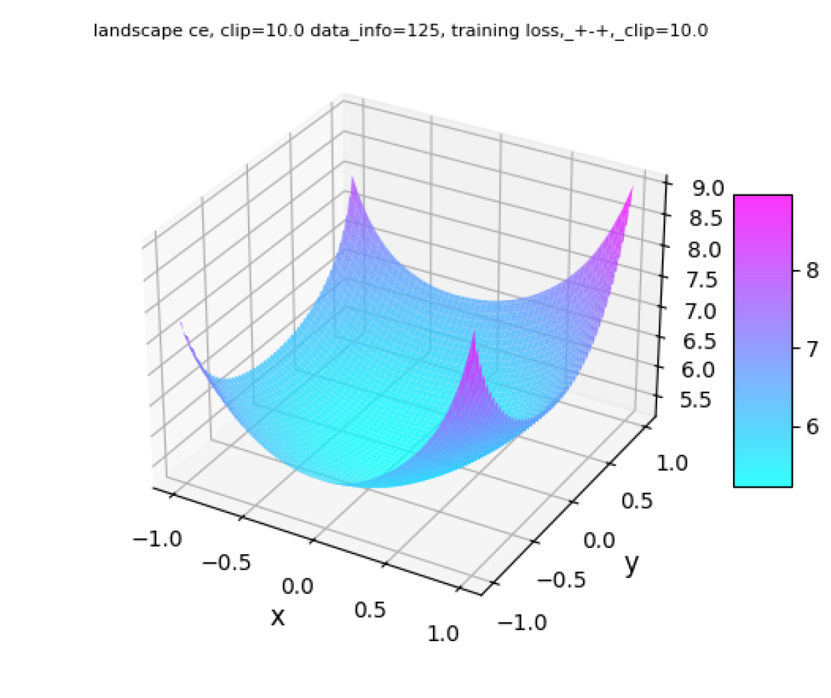
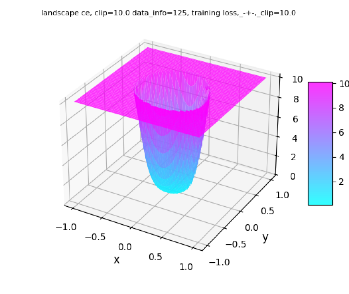
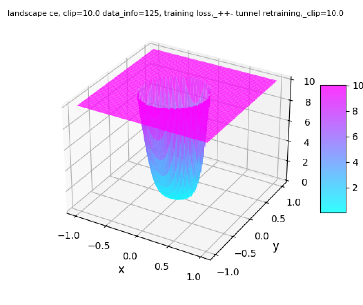
Figure 1: Training loss landscapes: comparison for Disjoint, Joint, and Mixed regimes (left to right)

As shown in Fig.  1 there is a significant difference in loss landscapes between the Disjoint regime and the Joint one. The Joint and Mixed regimes are similar in this regard.

In Appendix we show that in the disjoint regime, some head losses (usually early ones) do not have the local minimum for trained weights $\theta^{*}$ $((x,y)=(0,0))$ in the considered 3D subspace. The opposite is true for joint and mixed regimes. This fact coincides with much lower accuracy for early heads, as shown in Fig. 7. In Appendix we also include depictions for losses where $\delta$ and $\eta$ are sampled from uniform distribution. In this setting, mixed regime is characterized by smoother losses compared to joint regime showing that backbone pre-training may lead to easier optimization problem for early-exit architecture.

4.2 Numerical rank

To build a better understanding of early-exit training we look at the expressiveness of early-exit architectures under different regimes by means of numerical ranks. The rank of the internal representations, given the input, associated with different layers can provide insight into the "expressiveness" or capacity of the network. A higher rank (close to the maximum possible for a given layer’s matrix dimensions) indicates that the layer can capture more complex patterns or features in the data, as it implies a greater degree of linear independence among the feature detectors in that layer. High-rank activations matrices in a network suggest that the network is utilizing its capacity to learn diverse, high-frequency features, whereas a low rank might indicate that the network is not fully exploiting its potential.

In this framework, the numerical rank of the backbone architecture is analyzed under different early-exit regimes. A regular neural network is characterized by higher rank in earlier layers and lower one in later layers as shown in Fig.  2(a). Training only the backbone corresponds to the Phase 1 training. In Fig.  2(a) we can see the change in network expressiveness after adding intermediate classifiers and training the entire architecture jointly. Consequently, the numerical rank rises across the layers and becomes more uniform. This result indicates that early-exit architecture necessitates higher expressiveness of layers. See Appendix for more figures.

Fig.  2(b) shows the difference between the network trained with mixed and joint regime. The mixed regime has a flatter structure with relatively lower ranks earlier and higher ranks later. We hypothesize this since early-exit architecture consists of a set of classifiers placed uniformly across the network, the flatter architecture is desired for better performance across all the classifiers. In contrary, a steeper curve as in the case of joint regime may resemble more a regular architecture and be less suitable for early-exit task.

The numerical rank of matrices within a neural network not only provides insights into the computational and representational aspects but also influences the numerical stability and efficiency of training. Networks with appropriately constrained ranks are often easier to train and generalize better to unseen data.

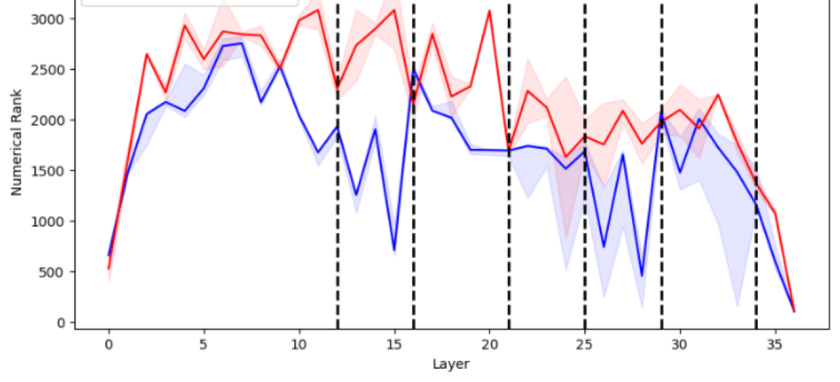
(a) The change in expressiveness of the network from Phase 1 (backbone) to Phase 2 (backbone+ICs).

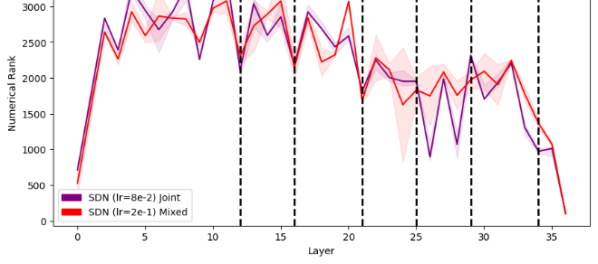
(b) Mixed vs joint training. The vertical lines indicate IC placement.

Figure 2: Numerical ranks of backbone network in an early-exit architecture trained with different regimes.

4.3 Mutual information.

In the context of neural networks, mutual information between $X$ and $Z$ represents how much information the input $X$ provides about the internal representation $Z$ after passing through a neural network.

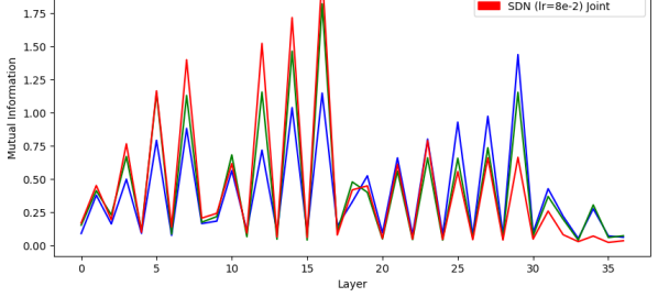
Figure 3: Mutual information $I(X;Z)$ between the input $X$ and the internal representation $Z$ for the ending training phase for regular backbone training, and mixed and joint early-exit training regimes.

[4] utilize the concept of mutual information between $X$ and $Z$ ($I(X;Z)$) in the framework of the information bottleneck (IB) principle. The IB principle aims to find a balance between the informativeness of the representation $Z$ for predicting the target variable $Y$ and the complexity of $Z$ in terms of its mutual information with the input $X$. Specifically, minimizing $I(X;Z)$ reduces the complexity and overfitting by ensuring $Z$ retains only the essential information from $X$, and maximizing $I(Y;Z)$ ensures that the representation $Z$ is informative enough to predict the target variable $Y$ effectively.

First, let us note the effect of early-exiting possibility on the mutual information. Due to exits, the mutual information between $X$ and $Z$ is smaller compared to a network trained without additional classifiers. Consequently, the network reduces the information in the final layers. Exiting earlier makes the information about the input less necessary in later layers since the decision is often made in the earlier parts of the architecture.

Following this observation, we note that the joint strategy is more suitable for easy datasets where more samples exit at earlier layers. Similarly, the mixed regime learns more uniform representation of the $I(X;Z)$ across the network (one may observe an analogy to the numerical rank results in the Sec. 4.2) and may be preferred for more difficult datasets that exit at later internal classifiers.

Moreover, as indicated in Fig. 3 training the backbone architecture in the mixed regime makes the mutual information closer to the information flow in the mixed regime more similar to the joint regime.

5 Empirical evaluation of training regimes.

General set-up.

Our model comparisons involve the CIFAR-10 [7], CIFAR-100 [7], Imagenette [9] and Imagenet [1] datasets. We perform our tests on the most established early-exit method SDN [5], and also verify our findings on GPF [12]. We train the standard ViT model from [6] on the CIFAR-10 dataset. We also train ResNet-34 [2] and EfficientNetV2-s [16] on the CIFAR-100 dataset. To test different pre-trained setting, we use the ViT-B [6] pretrained on ImageNet1k from Torchvision [13], and finetune it on CIFAR-100 dataset.

To ensure proper model training, we test different learning rates for pre-training the backbone and separately for each of the training phases, and select the optimal one for each phase and experimental set-up. For proper model convergence in each phase we utilize early-stopping to select a termination point of the training. This procedure halts training if there is no improvement in validation set accuracy over a specified number of epochs. At that point, we revert to the model checkpoint with the highest validation set accuracy.

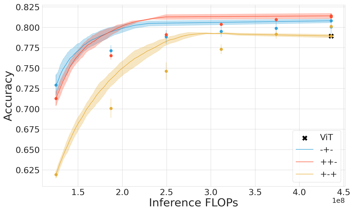
Figure 4: ViT and SDN performance in three training regimes

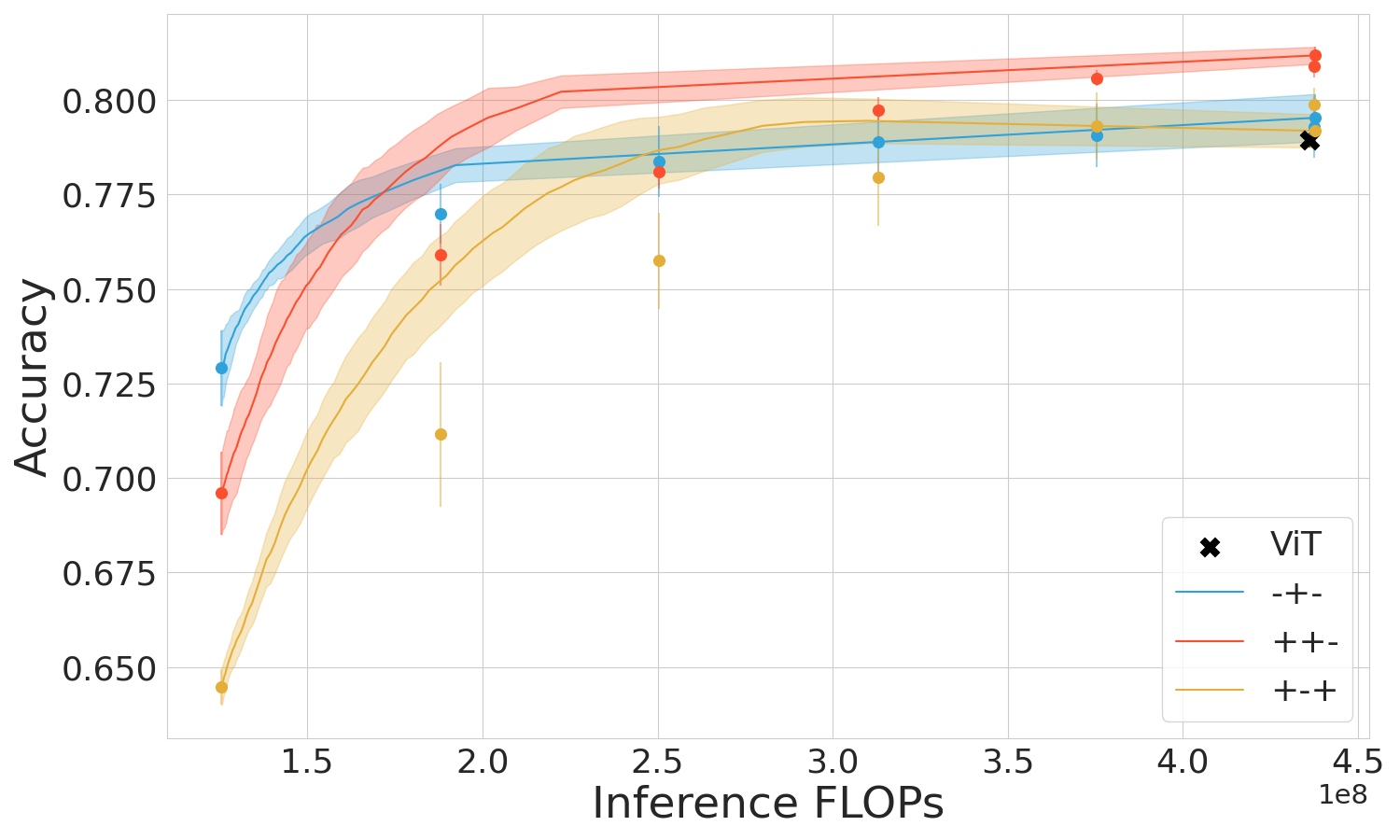
Figure 5: ViT and GPF peformance in three training regimes

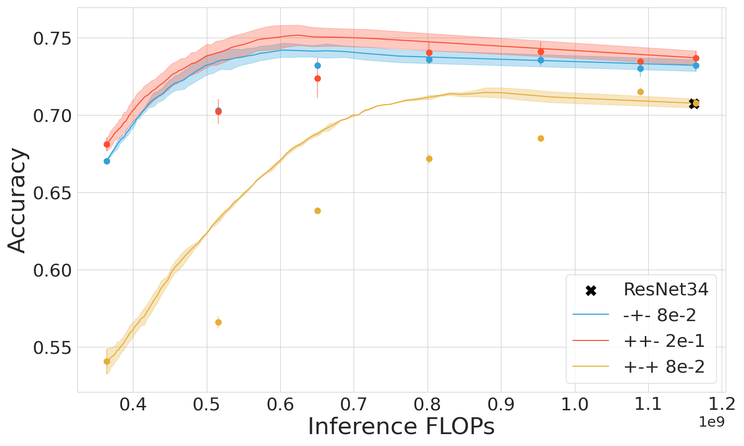
Figure 6: ResNet-34 and SDN performance in three training regimes

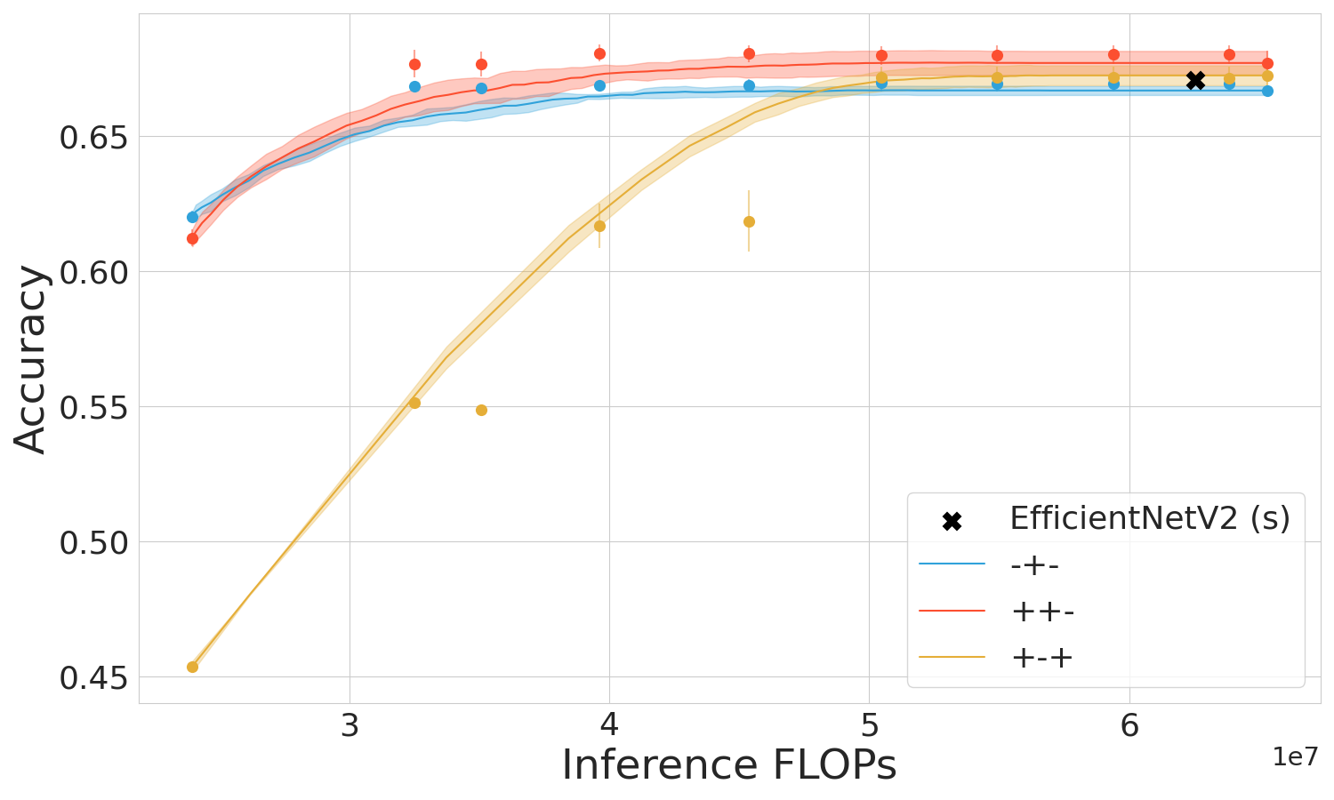
Figure 7: EfficientNetV2-s and SDN performance in three training regimes

Evaluation.

We assess each model by examining the trade-off between computational cost and task performance. For every early-exit model trained, we create 100 evenly spaced early-exit confidence thresholds, denoted as $\tau$. Then, we evaluate the model on the test set for each threshold and record the average FLOPs and classification accuracy. The trade-offs are aggregated for each method as a line on a two-dimensional plot, accompanied by its standard deviation. The standard deviation is calculated by conducting the experiment four times with different seeds.

In all the figures, a chosen training regime is encoded using three positions with signs + or -, where + indicates the phase included in training and - indicates the phase that is omitted. Hence, ++- denotes the mixed regime, -+- the joint training, and +-+ the disjoint training.

5.1 Efficiency trade-offs

In the ViT transformer model, we find that in both early-exit methods, mixed training achieves the best performance, see Fig. 7, 7. However, we should note that if exiting at very early stages (with low accuracy), a joint regime may be preferable. This effect is especially visible for GPF. In both methods training heads separately with frozen backbone yields the worst performance. In the case when ViT is pretrained with a different dataset (in our case, this is Imagenet) the conclusions are similar. The results are seen in Fig. 8. Mixed regime is shown to be the best performing across all computational budgets.

In the Resnet architecture, the results can be seen in Fig. 7. From the conducted experiments, it is evident that the disjoint regime is inferior compared to the rest. The difference between mixed and joint training is much smaller with a slight but consistent edge towards the mixed regime.

In EfficientNet setting seen in Fig. 7, in a similar way to Resnet-34, disjoint training is largely inferior. Mixed regime is consistently better across almost all computational budgets.

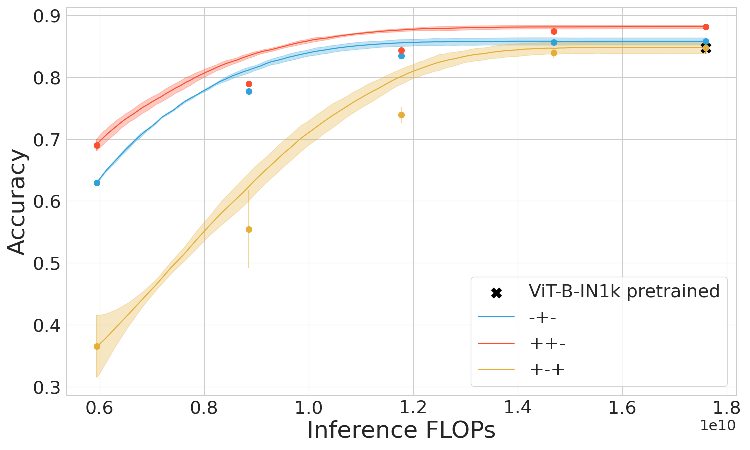
Figure 8: Performance of ViT-B pretrained on IN1k and SDN on CIFAR100 in 3 training regimes.

5.2 IC placement and size.

In this section, we look at two factors of variation in early exit architectures: internal classifier placement and the size of the classifier. There are no standard values that are given in literature. However, as shown below we note these factors play a role in the choice of training regime.

Frequency of IC classifiers. The frequency of internal classifiers in early exit architectures refers to how often these classifiers are inserted at different layers within the neural network. This can range from being placed at every layer to being placed at strategic intervals, depending on the architecture and the specific use case.

Placing internal classifiers at very frequent intervals (e.g., every layer) provides more opportunities for early exits, allowing the network to terminate inference earlier for simpler inputs. This can lead to significant computational savings, especially for easy-to-classify inputs. Placing internal classifiers less frequently (e.g., after every block or every few layers) can potentially lead to fewer computational savings but might be sufficient if the intermediate representations change significantly only after certain layers. Networks deployed in environments with highly variable input complexity might benefit from more frequent internal classifiers, providing more exit points to handle simpler inputs efficiently.

Table 1: The effect of varying head placement frequencies on the SDN early-exit architecture with ViT as a backbone, trained on Imagenette. Heads are placed after every $n$ layers. Given accuracy is obtained as in [18] using the time budget: 25%, 50%, 75%, 100% of the base network and without any limit (Max).

$n$	Regime	25%	50%	75%	100%	Max
$1$	mixed	$82.21$ $\pm 0.08$	$83.20$ $\pm 0.39$	$83.19$ $\pm 0.41$	$83.19$ $\pm 0.41$	$83.18$ $\pm 0.45$
	joint	$81.44$ $\pm 1.54$	$82.51$ $\pm 1.40$	$82.46$ $\pm 1.41$	$82.46$ $\pm 1.41$	$82.45$ $\pm 1.40$
	disjoint	$74.69$ $\pm 1.08$	$78.17$ $\pm 1.49$	$78.08$ $\pm 1.35$	$78.07$ $\pm 1.31$	$78.07$ $\pm 1.31$
$2$	mixed	$79.17$ $\pm 0.83$	$80.98$ $\pm 1.35$	$80.81$ $\pm 1.17$	$80.81$ $\pm 1.17$	$80.80$ $\pm 1.17$
	joint	$76.92$ $\pm 1.57$	$80.08$ $\pm 1.92$	$80.24$ $\pm 2.07$	$80.21$ $\pm 2.03$	$80.22$ $\pm 2.05$
	disjoint	$73.61$ $\pm 0.46$	$78.24$ $\pm 1.14$	$78.09$ $\pm 1.34$	$78.07$ $\pm 1.31$	$78.07$ $\pm 1.31$
$3$	mixed	$78.87$ $\pm 1.10$	$80.69$ $\pm 1.08$	$80.64$ $\pm 0.96$	$80.64$ $\pm 0.96$	$80.64$ $\pm 0.96$
	joint	$77.83$ $\pm 0.27$	$80.14$ $\pm 0.63$	$80.11$ $\pm 0.51$	$80.10$ $\pm 0.51$	$80.10$ $\pm 0.51$
	disjoint	$72.14$ $\pm 1.05$	$77.88$ $\pm 1.38$	$78.11$ $\pm 1.41$	$78.07$ $\pm 1.31$	$78.07$ $\pm 1.31$

As shown in the Table 1, training regimes perform differently when head frequencies vary. When heads are placed after each layer, the mixed regime outperforms the joint regime, especially when accounting for variation. With less frequent placements, performance drops and the difference between the joint and mixed regimes becomes less pronounced, although the mixed regime generally still prevails. Notably, the disjoint training regime shows the poorest performance of all.

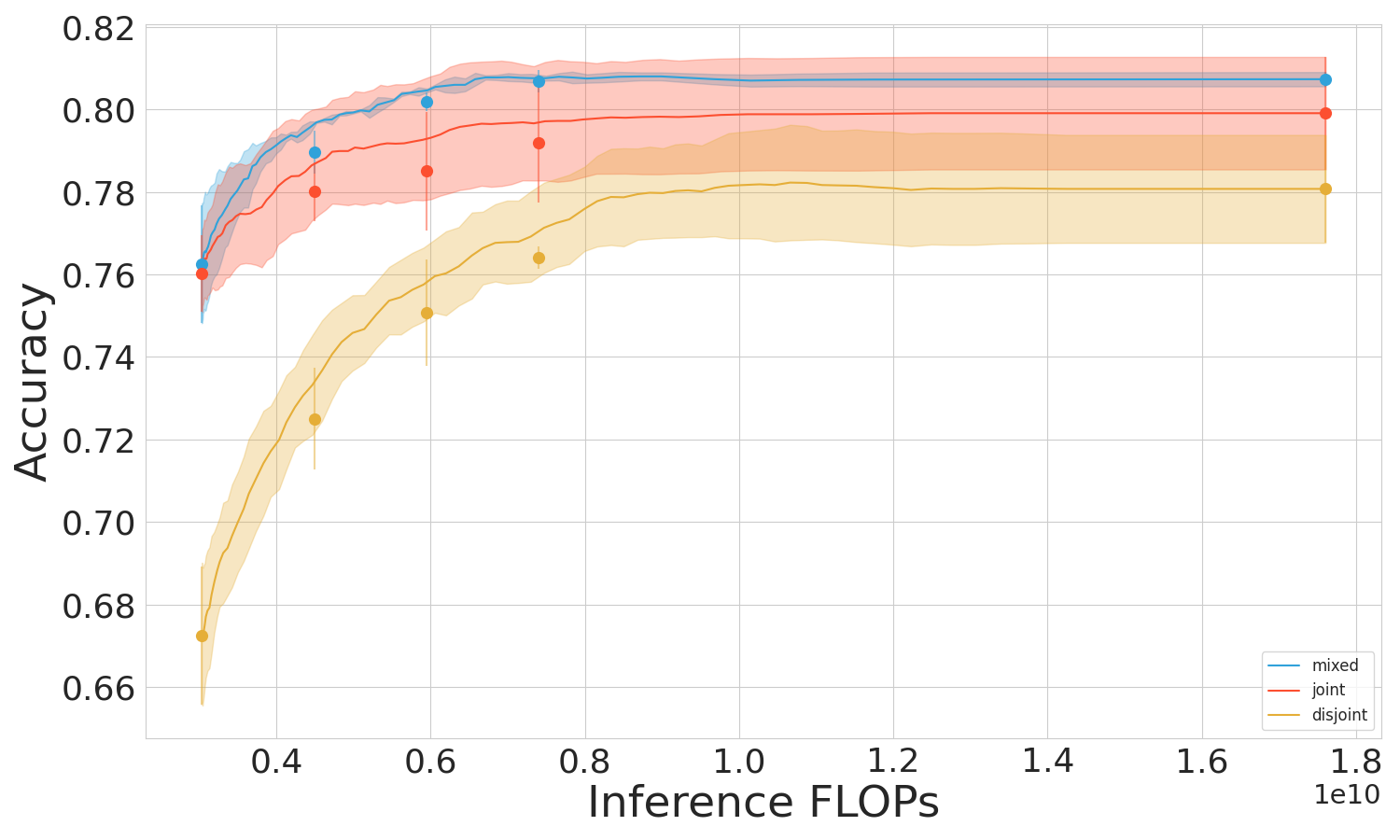
Figure 9: Performance when ICs are placed after each of the first $4$ layers.

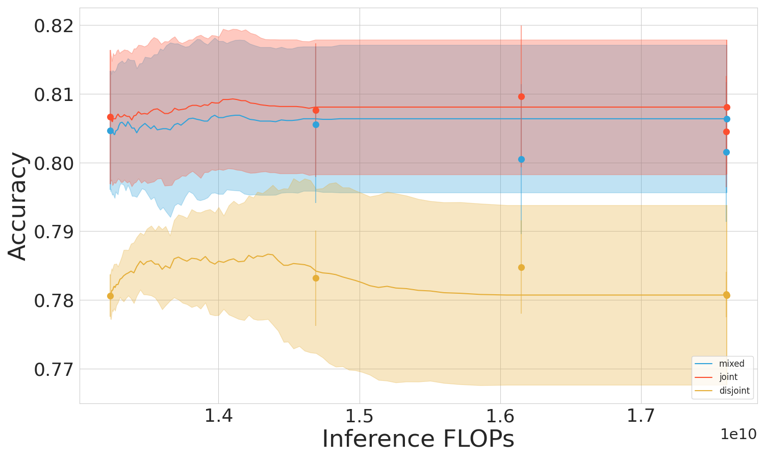
Figure 10: Performance when ICs are placed after each of the last $4$ layers.

We also examine where the heads are placed. As shown in Fig 10,10, networks trained with the mixed regime perform better than the joint regime when exits are positioned early in the network, while there is not much difference in accuracy in later sections. Moreover, we observe that when ICs are placed after each layer, most samples actually leave through earlier classifiers. In such cases, it is even more recommended to use the joint regime, which performs better for early classifiers.

Size of IC classifier. The size of an internal classifier in early exit architectures refers to the number of layers and neurons that make up the classifier inserted at intermediate layers of a neural network. The internal classifier typically consists of a few layers, such as a fully connected (dense) layer or a small convolutional block, although there is no standard IC architecture in literature.

The size of the internal classifier directly affects the computational cost of the early exit. Smaller internal classifiers are computationally cheaper and faster, enabling quick early exits without significant overhead. Larger internal classifiers, while potentially more accurate due to their increased capacity, may negate some of the computational savings achieved by early exits, especially if they are nearly as large as the remaining layers of the network.

We examine the effect of varying head sizes for the SDN architecture with ViT as the backbone. Each head architecture consists of either one or two connected layers with output dimensions of 1024 or 2048, followed by a softmax layer. As shown in Table 2, smaller architectures outperform larger ones. However, for larger architectures, there is a decrease in variation when using the joint training regime.

Table 2: The effect of varying head architecture size on the SDN early-exit architecture with ViT as a backbone, trained on Imagenette. Size describes number of layers used and output dimension.

Size	Regime	25%	50%	75%	100%	Max
1L-1024	mixed	$82.21$ $\pm 0.08$	$83.20$ $\pm 0.39$	$83.19$ $\pm 0.41$	$83.19$ $\pm 0.41$	$83.18$ $\pm 0.45$
	joint	$81.44$ $\pm 1.54$	$82.51$ $\pm 1.40$	$82.46$ $\pm 1.41$	$82.46$ $\pm 1.41$	$82.45$ $\pm 1.40$
2L-1024	mixed	$80.25$ $\pm 0.59$	$81.28$ $\pm 0.44$	$81.13$ $\pm 0.40$	$81.13$ $\pm 0.40$	$81.11$ $\pm 0.37$
	joint	$80.00$ $\pm 0.69$	$81.06$ $\pm 0.57$	$80.99$ $\pm 0.69$	$80.99$ $\pm 0.69$	$81.00$ $\pm 0.68$
2L-2048	mixed	$79.63$ $\pm 0.67$	$80.77$ $\pm 0.58$	$80.70$ $\pm 0.51$	$80.70$ $\pm 0.51$	$80.67$ $\pm 0.52$
	joint	$79.68$ $\pm 0.28$	$80.67$ $\pm 0.08$	$80.64$ $\pm 0.15$	$80.64$ $\pm 0.15$	$80.61$ $\pm 0.13$

5.3 How learning rate affects the training.

It is crucial to observe the effect of the learning rate choice on both performance and the comparison across all training strategies, in particular on proper backbone training. We make the following observations.

First, undertraining the backbone negatively affects mixed training setting. We perform identical experiments as described for ViT model but resulting in the undertrained backbone (trained with a learning rate $8\text{\times}{10}^{-4}$) ) achieving on average 77% accuracy. As shown in Fig. 12, when the backbone is undertrained mixed training underperforms and joint training yields a better outcome.

Secondly, as shown in Appendix, the learning rate also affects the second phase of mixed training. Then choosing a lower learning rate for the mixed training results in higher performance. However, a higher learning rate may perform better in low-resource settings when exiting at earlier classifiers.

In sum, we would like to state that it is important to have a properly trained backbone for the mixed training to perform better. To achieve this goal, unless we work in a very low-resource setting, lower learning rates are generally preferable.

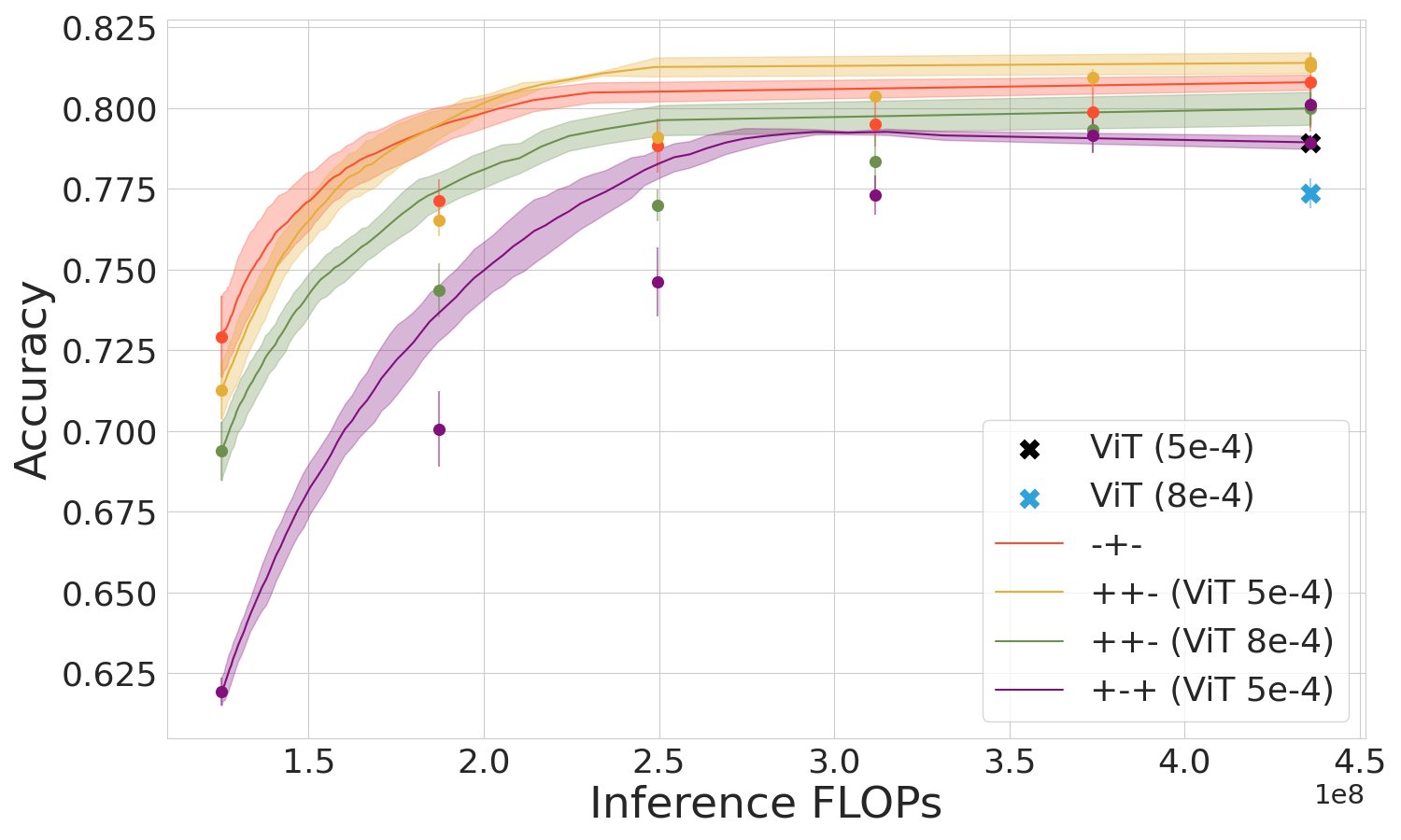
Figure 11: Mixed training performance drops with undertrained backbone (SDN, ViT)

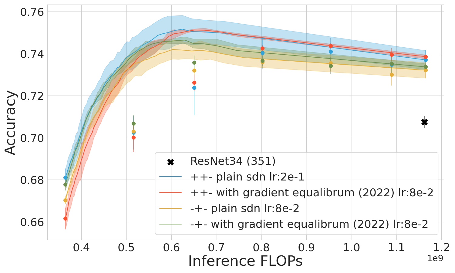
Figure 12: Comparison of chosen gradient scaling method with standard training (SDN) using the ResNet-34 model on CIFAR-100 across regimes.

5.4 Effects of gradient rescaling.

To effectively train the network and ICs, a weighted loss function is often used [20, 11]. This loss function $L$ accounts for the contributions of each IC’s prediction towards the overall objective. Weights can be adjusted to prioritize certain classifiers or to change the training dynamics over time.

The gradient scaling method is described by Eq. 2. The scaling involves multiplying the gradients of parameters $w_{n}$ of a given layer by the reciprocal of number of classifier, through which the input signal passes via that layer. There are $N-n+1$ such classifiers, where $N$ is the total number of classifiers and $n$ is the classifier number counting from the shallowest. This approach limits gradients and prevents a situation where all ICs would return the same signal for parameter improvement. In such a case, the same gradient would be amplified reinforcing such signals excessively.

$$\frac{\partial L}{\partial w_{n}}=\frac{1}{N-n+1}\sum_{i=n}^{N}\frac{\partial L_{i}}{\partial w_{n}},$$ (2)

We compare the conventional early-exit training method with the gradient-scaling version across regimes, the results can be seen in Fig. 12. For deeper classifiers, we can observe that in mixed regimes we cannot definitively say that the selected gradient scaling method alters the performance and offers some improvement for the joint regime. For shallower ones the performance degrades in the mixed regime, and improves in the joint regime. Overall, even with the scaling that may benefit the joint regime, the mixed training remains superior.

6 Discussion

In conclusion, this paper presents a comprehensive analysis and evaluation of different training regimes for early-exit models in deep neural networks. By categorizing training approaches into disjoint, joint, and mixed regimes, we have demonstrated that the way the backbone and internal classifiers in early-exit architectures are trained influences its performance and efficiency.

Among the benchmark methods, the mixed training regime is preferable in most of the cases. This method ensures that the backbone network is well-optimized before the integration of internal classifiers, leading to improved computational efficiency and accuracy. Mixed regime also hints at using pre-trained models as backbones in early-exit architectures. Both the theoretical and empirical findings show the mixed regime should be selected for easy and varying input complexity datasets with many samples exiting at earlier layers. In other cases the joint training can be preferable for harder datasets where samples leave by rear classifiers.

Future research should investigate more sophisticated optimization techniques, such as adaptive learning rates or meta-learning strategies, specifically designed for early-exit models. Moreover, other training strategies may be proposed where training is tailored to particular sub-networks within the entire early-exit architecture.

Overall, this study contributes valuable insights into the training of early-exit models, providing a foundation for developing more efficient dynamic deep learning systems.

References

- [1] Jia Deng, Wei Dong, Richard Socher, Li-Jia Li, Kai Li, and Li Fei-Fei. Imagenet: A large-scale hierarchical image database. In 2009 IEEE conference on computer vision and pattern recognition, pages 248–255. Ieee, 2009.
- [2] Kaiming He, Xiangyu Zhang, Shaoqing Ren, and Jian Sun. Deep residual learning for image recognition. In Proceedings of the IEEE conference on computer vision and pattern recognition, pages 770–778, 2016.
- [3] Gao Huang, Danlu Chen, Tianhong Li, Felix Wu, Laurens van der Maaten, and Kilian Q. Weinberger. Multi-scale dense networks for resource efficient image classification. In International Conference on Learning Representations, 2018.
- [4] Kenji Kawaguchi, Zhun Deng, Xu Ji, and Jiaoyang Huang. How does information bottleneck help deep learning? In International Conference on Machine Learning, pages 16049–16096. PMLR, 2023.
- [5] Yigitcan Kaya, Sanghyun Hong, and Tudor Dumitras. Shallow-deep networks: Understanding and mitigating network overthinking. In Proceedings of the International Conference on Machine Learning, ICML, pages 3301–3310, 2019.
- [6] Alexander Kolesnikov, Alexey Dosovitskiy, Dirk Weissenborn, Georg Heigold, Jakob Uszkoreit, Lucas Beyer, Matthias Minderer, Mostafa Dehghani, Neil Houlsby, Sylvain Gelly, Thomas Unterthiner, and Xiaohua Zhai. An image is worth 16x16 words: Transformers for image recognition at scale. 2021.
- [7] Alex Krizhevsky, Vinod Nair, and Geoffrey Hinton. Cifar-10 (canadian institute for advanced research).
- [8] Assaf Lahiany and Yehudit Aperstein. Pteenet: Post-trained early-exit neural networks augmentation for inference cost optimization. IEEE Access, 10:69680–69687, 2022.
- [9] Ya Le and Xuan S. Yang. Tiny imagenet visual recognition challenge. 2015.
- [10] Hao Li, Zheng Xu, Gavin Taylor, Christoph Studer, and Tom Goldstein. Visualizing the loss landscape of neural nets. Advances in neural information processing systems, 31, 2018.
- [11] Hao Li, Hong Zhang, Xiaojuan Qi, Yang Ruigang, and Gao Huang. Improved techniques for training adaptive deep networks. In 2019 IEEE/CVF International Conference on Computer Vision (ICCV), pages 1891–1900, 2019.
- [12] Kaiyuan Liao, Yi Zhang, Xuancheng Ren, Qi Su, Xu Sun, and Bin He. A global past-future early exit method for accelerating inference of pre-trained language models. In Proceedings of the 2021 Conference of the North American Chapter of the Association for Computational Linguistics: Human Language Technologies, pages 2013–2023, 2021.
- [13] TorchVision maintainers and contributors. Torchvision: Pytorch’s computer vision library. https://github.com/pytorch/vision, 2016.
- [14] Lassi Meronen, Martin Trapp, Andrea Pilzer, Le Yang, and Arno Solin. Fixing overconfidence in dynamic neural networks. In Proceedings of the IEEE/CVF Winter Conference on Applications of Computer Vision, pages 2680–2690, 2024.
- [15] Priyadarshini Panda, Abhronil Sengupta, and Kaushik Roy. Conditional deep learning for energy-efficient and enhanced pattern recognition. In 2016 Design, Automation & Test in Europe Conference & Exhibition (DATE), pages 475–480. IEEE, 2016.
- [16] Mingxing Tan and Quoc V. Le. Efficientnetv2: Smaller models and faster training. CoRR, abs/2104.00298, 2021.
- [17] Surat Teerapittayanon, Bradley McDanel, and Hsiang-Tsung Kung. Branchynet: Fast inference via early exiting from deep neural networks. In Proceedings of the International Conference on Pattern Recognition, ICPR, pages 2464–2469, 2016.
- [18] Bartosz Wójcik, Marcin Przewieźlikowski, Filip Szatkowski, Maciej Wołczyk, Klaudia Bałazy, Bartłomiej Krzepkowski, Igor Podolak, Jacek Tabor, Marek Śmieja, and Tomasz Trzciński. Zero time waste in pre-trained early exit neural networks. Neural Networks, 168:580–601, 2023.
- [19] Le Yang, Yizeng Han, Xi Chen, Shiji Song, Jifeng Dai, and Gao Huang. Resolution adaptive networks for efficient inference. In 2020 IEEE/CVF Conference on Computer Vision and Pattern Recognition (CVPR), pages 2369–2378, 2020.
- [20] Haichao Yu, Haoxiang Li, Gang Hua, Gao Huang, and Humphrey Shi. Boosted dynamic neural networks. In arXiv preprint arXiv:2211.16726, 2022.
- [21] Wangchunshu Zhou, Canwen Xu, Tao Ge, Julian McAuley, Ke Xu, and Furu Wei. BERT loses patience: fast and robust inference with early exit. arXiv:2006.04152, 2020.