Subsampled One-Step Estimation for Fast Statistical Inference
Abstract
Subsampling is an effective approach to alleviate the computational burden associated with large-scale datasets. Nevertheless, existing subsampling estimators incur a substantial loss in estimation efficiency compared to estimators based on the full dataset. Specifically, the convergence rate of existing subsampling estimators is typically rather than , where and denote the subsample and full data sizes, respectively. This paper proposes a subsampled one-step (SOS) method to mitigate the estimation efficiency loss utilizing the asymptotic expansions of the subsampling and full-data estimators. The resulting SOS estimator is computationally efficient and achieves a fast convergence rate of rather than . We establish the asymptotic distribution of the SOS estimator, which can be non-normal in general, and construct confidence intervals on top of the asymptotic distribution. Furthermore, we prove that the SOS estimator is asymptotically normal and equivalent to the full data-based estimator when . Simulation studies and real data analyses were conducted to demonstrate the finite sample performance of the SOS estimator. Numerical results suggest that the SOS estimator is almost as computationally efficient as the uniform subsampling estimator while achieving similar estimation efficiency to the full data-based estimator.
Keywords: Large-scale data; One-step estimation; Statistical efficiency; Subsampling.
1 Introduction
In recent years, big data has attracted great attention in various fields. Big data provides statisticians with the opportunity to explore vast amounts of information. However, traditional statistical methods can be computationally cumbersome or even infeasible with large-scale datasets. Existing methods for processing big data can be divided into three categories: distributed methods (Mcdonald et al., 2009; Zhang et al., 2013; Lee et al., 2017; Jordan et al., 2019), online update methods (Lin and Xi, 2011; Schifano et al., 2016; Luo and Song, 2020; Luo et al., 2023), and subsampling methods (Drineas et al., 2006, 2011; Fithian and Hastie, 2014; Ma et al., 2015; Ma and Sun, 2015; Han et al., 2020; Wang et al., 2018, 2019; Yao and Wang, 2019; Wang and Ma, 2020; Yu et al., 2020; Ai et al., 2021a, b). Distributed methods necessitate parallel computing systems, thus having high requirements for equipment. On the other hand, online update methods primarily cater to streaming data scenarios. Compared to distributed and online updating algorithms, subsampling techniques have become prevalent in numerous real-world applications due to their computational efficiency and their ability to be implemented with minimal computational resources, e.g., a single laptop. This article mainly focuses on the subsampling strategy.
The main issue of the subsampling strategy is that it only uses a small part of the data, making it hard to attain the estimation efficiency of the full data-based estimator (Drineas et al., 2006; Kushilevitz and Nisan, 1996). Therefore, many works are devoted to improving the estimation efficiency of subsampling estimation. The rationale behind many existing subsampling improvement strategies is that the information contained in different observations is different, and observations with more information should be sampled with higher probability (Wang, 2019). Based on this idea, many improvement schemes focus on designing nonuniform sampling probability (NSP) to improve the estimation efficiency of subsampling estimators. Drineas et al. (2006) proposed a leverage subsampling method for linear models, which prefers to select leverage points. Drineas et al. (2011) and Ma et al. (2015) proposed some fast calculation algorithms to speed up the calculation of the leverage subsampling method. Fithian and Hastie (2014) proposed a local case-control subsampling method for logistic regression, which prefers to keep data points which are easily misclassified. Han et al. (2020) extended the idea in Fithian and Hastie (2014) to the multi-class classification problem. These methods design subsampling probability based on some intuitive sample importance. Another line of work is the variance-based subsampling methods that design the NSP to minimize some criterion function of the resulting estimator’s asymptotic variance (Wang et al., 2018). This idea has been developed to dealing with various problems including the multi-class logistic regression (Yao and Wang, 2019), the quantile regression (Ai et al., 2021b), the quasi-likelihood (Yu et al., 2020), and cox regression (Keret and Gorfine, 2023). Recently, Fan et al. (2022) proposes an empirical likelihood weighting method that improves the estimation efficiency of the subsampling estimator by incorporating some easily available auxiliary information. The above estimators converge to the true parameter at the rate , where is the subsample size. Typically, is much smaller than the sample size of the full data . Thus, these subsampling estimators still has substantial estimation efficiency loss compared to the full data-based estimator.
This paper proposes a new approach to mitigating the estimation efficiency loss in subsampling M-estimator. The proposed method is based on uniform subsampling which includes different observations with equal probability. We commence by investigating the asymptotic expansions of the uniformly subsampled and full data-based estimators, subsequently devising a subsampled one-step (SOS) method to improve the estimation efficiency of the uniformly subsampled estimator while maintaining the computational efficiency. We prove that the SOS estimator has a fast convergence rate rather than . We establish the asymptotic distribution of the proposed estimator which can be non-normal in general. The confidence interval is provided for statistical inference based on the asymptotic distribution of SOS. Furthermore, we prove that the SOS estimator is asymptotically as efficient as the full data-based estimator when . Extensive numerical experiments were conducted based on both simulated and real datasets to demonstrate the finite sample performance of the proposed estimator. The proposed estimator exhibits promising performance in terms of both estimation efficiency and computational efficiency in our numerical results.
The rest of this paper is organized as follows. In Section 2, we introduce the SOS method. In Section 3, we establishes the asymptotic properties of the SOS estimator. In Section 4, we conduct simulation studies to evaluate the finite sample performance of the SOS estimator in terms of estimation efficiency and computation efficiency. Furthermore, we present a real data example in Section 5 to illustrate the practical application of the SOS method. The proofs are delayed to Appendix.
2 Methodology
Let be independent and identically distributed observations of a random vector . Suppose the parameter of interest is the minimizer of the population loss function , that is,
where is the parameter space. A natural estimator for can be obtained by minimizing the sample version of . Specifically, the full data-based M-estimator is
Computation of the full data-based estimator is time-consuming when dealing with extremely large datasets, particularly in cases where does not have a closed-form solution and requires to be solved by an iterative algorithm. The computing time of is of order when employing the Newton-Raphson algorithm, where denotes the number of iterations. When the sample size is large, storing the data and computing the full data-based estimator can be challenging or even infeasible.
Subsampling provides an effective approach to reduce the computational burden associated with large-scale data. The simplest subsampling is the uniform subsampling, which is also computationally efficient. The uniform subsampling method involves generating a Bernoulli random variable for each data point with , where represents the expected subsample size. Let denote the index set of the subsample. Based on the subsample indexed by , the uniform subsampling M-estimator can be defined as:
| (1) |
The uniform subsampling estimator is computationally efficient, while it is not as accurate as the full data-based estimator since only a small portion of the data is used. Extensive studies devote to improving the estimation efficiency of (Drineas et al., 2006; Yu et al., 2020; Yao and Wang, 2019; Wang et al., 2018, 2019; Wang and Ma, 2020; Ai et al., 2021a). However, the convergence rate of the existing estimator is typically , which can be much slower than that of .
This paper aims to develop a computationally and statistically efficient estimator that can asymptotically achieve the same estimation efficiency as the full data-based estimator while retaining similar computing time as . Note that under regularity conditions, the full-data based estimator and the uniform subsampling have the following asymptotic expansions
| (2) |
and
| (3) |
respectively. By comparing the expansions in (2) and (3), we have
| (4) |
One can find that the second term at the right side of (4) is ignorable when , i.e., the susbample size is not too small. The estimation efficiency loss comes mainly from the first term on the right side of (4), which is of order .
To mitigate the estimation efficiency loss while maintaining computational efficiency, we construct an easy-to-compute estimate for the first term on the right side of (4). Specifically, we estimate and by and
respectively. Then, we define the SOS estimator as
Notice that the computation of only involves sample average over the full data, which is easy to calculate even for large-scale data. The time complexity for computing is that is of the same order as that of computing the NSP for existing subsampling methods (Wang, 2019; Wang and Ma, 2020). In the next section, we establish the asymptotic properties of the SOS estimator.
3 Asymptotic Properties
In this section, we establish the asymptotic properties of the proposed estimator . For this purpose, we consider the following regularity conditions.
-
(C1)
There exist and such that , , and for any , with for .
-
(C2)
There exists some such that , , and .
-
(C3)
The minimum eigenvalue of is bounded away from zero.
Theorem 1.
Under conditions (C1)–(C3), as , we have
and
| (5) |
where is a dimensional random vector following from with
, with , with being the vectorized form of the upper triangle of , , , , , , and
, , the notation denotes Kronecker product, consists of the first elements of , consists of the -th to the -th elements of , and is a symmetrical matrix with upper triangle matrix consisted by the elements in arranged in rows with consisting of the -th to the -th elements of , is a matrix with the -th row being the vectorized form of the Hessian matrix of , and .
Theorem 1 shows that the convergence rate of is , significantly faster than the existing subsampling estimators whose convergence rates are typically of order (Wang et al., 2018; Wang and Ma, 2020; Yu et al., 2020). In addition, Theorem 1 establishes the asymptotic distribution of . Although the SOS is motivated by the asymptotic expansion under the assumption that , asymptotic properties of the SOS estimator can be derived with no condition on the ratio between and . Previous works, such as those by Su et al. (2022) and Wang et al. (2024), often assume to derive asymptotic distributions for subsampling estimators. However, it may be hard to process a subsample of size if the computational source is limited and the is extremely large. Our results facilitate inference even when is not significantly larger than , providing a practical solution for situations with limited computational resources.
The confidence interval for the proposed SOS estimator can be constructed based on the Monte Carlo approximation of the asymptotic distribution in Theorem 1 as follows:
-
Step 1.
Estimate by which replaces the expectation in by the corresponding sample form based on the subsample indexed by and replaces by ;
-
Step 2.
Generate random samples from the normal distribution with mean and variance ;
-
Step 3.
Estimate and in Theorem 1 by and , respectively, which replaces the expectation in and by their sample form based on the subsample indexed by and replaces in and by ;
-
Step 4.
Estimate by which replaces and in by and , respectively, and calculate for ;
-
Step 5.
Determine the lower and upper quantiles of , denoted by and respectively, where is the -th component of for and ;
-
Step 6.
For , construct the confidence interval for with confidence level as .
See Section 4 for the numerical performance of the proposed confidence interval. The asymptotic distribution in (5) is complicated and which requires to be approximated by the Monte Carlo approximation. The asymptotic distribution can be greatly simplified when the subsample size is not too small compared to the full data size in the sense that . In this case, is asymptotically equivalent to the full data-based estimator .
Theorem 2.
4 Numerical Experiments
In this section, we conduct numerical experiments to evaluate the finite sample performance of the proposed method. For comparison, we also calculate several other subsampling estimators, including the uniform subsampling estimator (UNI) in (1), the inverse probability weighted subsampling estimator (IPW) with the optimal nonuniform subsampling probability (optNSP) that minimizes the asymptotic mean squared error of the IPW estimator, the optNSP-based maximum sampled conditional likelihood subsampling estimator (MSCL), and the optNSP-based empirical likelihood weighting subsampling estimator (ELW). As a reference, we also calculate the full data-based estimator (FULL).
In the simulation, we generate a set of i.i.d. observations , , where is a -dimensional covariate vector, and are independently generated from . We consider two regression models: logistic regression and Weibull regression. In the logistic regression model, the response variable follows a Bernoulli distribution with mean , where and is a -dimensional vector with all elements set to . The parameter of interest is . In the Weibull regression model, the response variable is generated as , where follows a Weibull distribution with a shape parameter and scale parameter . The parameter of interest is . For each of the models, we fix the full sample size and vary the subsample size to be , , and . In addition, to calculate the optNSP, we generate a pilot sample of size . To evaluate the performance of an estimator , we calculate its empirical based on repetitions, where is the estimate from the -th run. Figure 1 plots the RMSE of above estimators under the logistic and Weibull models for different subsample sizes. Due to computational complexity, we do not provide the results for the MSCL estimator under the Weibull model, as the integral operation involved in this estimator is difficult to express in closed form.
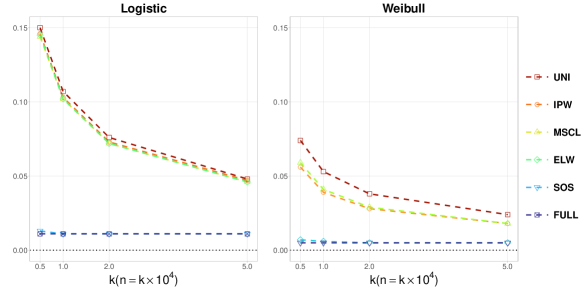
Figure 1 shows that the UNI subsampling estimator exhibits a large RMSE. The IPW, MSCL, and ELW estimators under the logistic model and the IPW and ELW estimators under the Weibull model have smaller RMSE than the UNI estimator, and the estimation efficiency improvement is significant under the Weibull model. Nevertheless, these subsampling estimators still suffer from substantial estimation efficiency loss compared to the full data-based estimator. In contrast, the proposed SOS estimator outperforms other subsampling estimators in terms of RMSE and even performs similarly to the full data-based estimator under both models. This phenomenon aligns with our theoretical results in Theorems 1–2. The proposed estimator achieves a faster convergence rate than existing subsampling estimators and even has the same estimation efficiency as the full data-based estimator when the subsample size is not too small compared to the full data size.
To further evaluate these estimators, we present the bias and the Monte Carlo standard deviation (SD) of above estimators for each dimension under the logistic and Weibull models in Tables 1 and 2, respectively. The bias and SD of the full data based estimator do not change as the subsample size varies and hence we present the results here. The bias and SD of the full data based estimator under the logistic model are (0.000, -0.003, 0.000, -0.001, 0.000, 0.001, 0.001, 0.000, -0.001, 0.002) and (0.020, 0.035, 0.035, 0.036, 0.035, 0.037, 0.034, 0.036, 0.036, 0.036), respectively. The bias and SD of the full data based estimator under the Weibull model are (0.000, 0.000, 0.001, 0.000, 0.000, 0.000, -0.001, -0.001, 0.000, -0.001, -0.001) and (0.004, 0.010, 0.017, 0.017, 0.018, 0.017, 0.018, 0.017, 0.017, 0.018, 0.017), respectively.
| UNI | IPW | MSCL | ELW | SOS | |||||||
|---|---|---|---|---|---|---|---|---|---|---|---|
| Bias | SD | Bias | SD | Bias | SD | Bias | SD | Bias | SD | ||
| 0.5 | 1 | 0.009 | 0.292 | -0.008 | 0.276 | -0.010 | 0.273 | 0.001 | 0.057 | 0.000 | 0.025 |
| 2 | 0.030 | 0.489 | -0.019 | 0.477 | -0.015 | 0.466 | -0.017 | 0.478 | -0.006 | 0.043 | |
| 3 | 0.011 | 0.489 | -0.016 | 0.500 | -0.010 | 0.494 | -0.002 | 0.485 | -0.005 | 0.043 | |
| 4 | 0.026 | 0.481 | -0.012 | 0.474 | -0.006 | 0.468 | 0.019 | 0.475 | -0.006 | 0.041 | |
| 5 | 0.008 | 0.498 | -0.007 | 0.477 | -0.006 | 0.471 | 0.005 | 0.484 | -0.006 | 0.042 | |
| 6 | -0.005 | 0.478 | 0.013 | 0.488 | 0.017 | 0.479 | 0.017 | 0.499 | -0.003 | 0.044 | |
| 7 | 0.005 | 0.504 | -0.011 | 0.475 | -0.010 | 0.470 | 0.006 | 0.504 | -0.003 | 0.041 | |
| 8 | -0.001 | 0.505 | -0.011 | 0.451 | -0.009 | 0.444 | 0.005 | 0.472 | -0.005 | 0.044 | |
| 9 | 0.028 | 0.480 | -0.031 | 0.479 | -0.032 | 0.474 | -0.007 | 0.465 | -0.005 | 0.042 | |
| 10 | 0.019 | 0.500 | 0.002 | 0.468 | -0.002 | 0.463 | 0.037 | 0.479 | -0.003 | 0.044 | |
| 1 | |||||||||||
| 1 | 0.003 | 0.204 | -0.004 | 0.192 | -0.004 | 0.189 | 0.001 | 0.043 | 0.000 | 0.021 | |
| 2 | 0.011 | 0.345 | -0.001 | 0.339 | -0.002 | 0.332 | -0.008 | 0.333 | -0.005 | 0.037 | |
| 3 | 0.002 | 0.345 | -0.014 | 0.346 | -0.009 | 0.339 | -0.009 | 0.344 | -0.002 | 0.037 | |
| 4 | 0.011 | 0.355 | -0.002 | 0.339 | 0.000 | 0.337 | 0.015 | 0.348 | -0.004 | 0.037 | |
| 5 | 0.003 | 0.344 | -0.010 | 0.336 | -0.011 | 0.333 | -0.001 | 0.335 | -0.003 | 0.037 | |
| 6 | 0.013 | 0.356 | -0.003 | 0.347 | -0.001 | 0.343 | 0.004 | 0.338 | -0.001 | 0.039 | |
| 7 | -0.003 | 0.350 | -0.004 | 0.324 | -0.006 | 0.322 | 0.007 | 0.349 | -0.001 | 0.036 | |
| 8 | 0.007 | 0.360 | -0.007 | 0.341 | -0.005 | 0.336 | -0.008 | 0.341 | -0.002 | 0.038 | |
| 9 | 0.011 | 0.341 | -0.013 | 0.342 | -0.014 | 0.335 | 0.001 | 0.348 | -0.004 | 0.038 | |
| 10 | 0.008 | 0.359 | -0.013 | 0.331 | -0.015 | 0.325 | 0.017 | 0.331 | 0.000 | 0.039 | |
| 2 | |||||||||||
| 1 | -0.002 | 0.147 | 0.001 | 0.142 | 0.002 | 0.140 | 0.000 | 0.032 | 0.000 | 0.020 | |
| 2 | -0.008 | 0.252 | 0.005 | 0.231 | 0.005 | 0.227 | -0.011 | 0.235 | -0.004 | 0.036 | |
| 3 | 0.005 | 0.243 | -0.006 | 0.241 | -0.004 | 0.238 | 0.006 | 0.233 | -0.001 | 0.035 | |
| 4 | 0.009 | 0.250 | -0.007 | 0.241 | -0.005 | 0.237 | 0.011 | 0.244 | -0.002 | 0.036 | |
| 5 | 0.003 | 0.246 | 0.001 | 0.240 | 0.001 | 0.239 | -0.010 | 0.239 | -0.001 | 0.035 | |
| 6 | 0.007 | 0.254 | 0.008 | 0.236 | 0.009 | 0.233 | 0.004 | 0.233 | 0.000 | 0.038 | |
| 7 | -0.007 | 0.253 | 0.009 | 0.247 | 0.008 | 0.242 | 0.002 | 0.252 | 0.000 | 0.035 | |
| 8 | -0.009 | 0.250 | -0.009 | 0.242 | -0.006 | 0.239 | 0.000 | 0.236 | -0.001 | 0.036 | |
| 9 | -0.001 | 0.247 | -0.008 | 0.240 | -0.008 | 0.236 | 0.010 | 0.239 | -0.002 | 0.037 | |
| 10 | 0.004 | 0.251 | -0.021 | 0.234 | -0.021 | 0.230 | 0.021 | 0.241 | 0.001 | 0.037 | |
| 5 | |||||||||||
| 1 | 0.001 | 0.090 | 0.002 | 0.089 | 0.002 | 0.088 | 0.000 | 0.025 | 0.000 | 0.020 | |
| 2 | -0.006 | 0.160 | -0.003 | 0.150 | -0.003 | 0.148 | 0.007 | 0.149 | -0.003 | 0.035 | |
| 3 | 0.006 | 0.148 | 0.003 | 0.156 | 0.004 | 0.154 | 0.008 | 0.150 | 0.000 | 0.035 | |
| 4 | -0.001 | 0.162 | -0.007 | 0.154 | -0.006 | 0.152 | 0.000 | 0.146 | -0.002 | 0.036 | |
| 5 | -0.003 | 0.160 | -0.001 | 0.151 | -0.001 | 0.150 | -0.006 | 0.155 | -0.001 | 0.035 | |
| 6 | 0.000 | 0.161 | 0.004 | 0.146 | 0.004 | 0.144 | 0.001 | 0.150 | 0.000 | 0.037 | |
| 7 | -0.002 | 0.162 | 0.001 | 0.152 | 0.001 | 0.149 | 0.002 | 0.156 | 0.000 | 0.034 | |
| 8 | 0.002 | 0.156 | 0.000 | 0.155 | 0.000 | 0.153 | -0.001 | 0.154 | -0.001 | 0.036 | |
| 9 | -0.001 | 0.155 | -0.006 | 0.150 | -0.008 | 0.149 | 0.003 | 0.151 | -0.001 | 0.036 | |
| 10 | 0.006 | 0.160 | -0.013 | 0.156 | -0.012 | 0.154 | 0.009 | 0.154 | 0.001 | 0.036 | |
| UNI | IPW | ELW | SOS | ||||||
|---|---|---|---|---|---|---|---|---|---|
| Bias | SD | Bias | SD | Bias | SD | Bias | SD | ||
| 0.1 | 1 | 0.007 | 0.055 | 0.000 | 0.057 | 0.002 | 0.041 | -0.007 | 0.005 |
| 2 | -0.001 | 0.153 | 0.000 | 0.123 | -0.001 | 0.111 | -0.004 | 0.012 | |
| 3 | -0.003 | 0.241 | 0.008 | 0.180 | 0.011 | 0.186 | -0.002 | 0.024 | |
| 4 | 0.003 | 0.244 | 0.003 | 0.184 | 0.002 | 0.190 | -0.002 | 0.024 | |
| 5 | 0.001 | 0.237 | 0.007 | 0.180 | -0.007 | 0.194 | -0.003 | 0.024 | |
| 6 | 0.005 | 0.248 | 0.005 | 0.184 | -0.004 | 0.191 | -0.002 | 0.023 | |
| 7 | -0.006 | 0.239 | -0.001 | 0.185 | 0.000 | 0.192 | -0.003 | 0.024 | |
| 8 | 0.004 | 0.237 | -0.006 | 0.181 | 0.004 | 0.195 | -0.004 | 0.023 | |
| 9 | 0.012 | 0.245 | -0.005 | 0.179 | 0.006 | 0.197 | -0.002 | 0.025 | |
| 10 | -0.005 | 0.243 | 0.008 | 0.185 | 0.005 | 0.193 | -0.002 | 0.023 | |
| 11 | 0.007 | 0.238 | 0.008 | 0.173 | -0.010 | 0.188 | -0.003 | 0.024 | |
| 0.5 | |||||||||
| 1 | 0.003 | 0.040 | -0.001 | 0.040 | 0.001 | 0.029 | -0.004 | 0.004 | |
| 2 | 0.000 | 0.106 | 0.002 | 0.088 | 0.000 | 0.078 | -0.002 | 0.011 | |
| 3 | -0.002 | 0.173 | 0.005 | 0.126 | 0.004 | 0.131 | 0.000 | 0.019 | |
| 4 | 0.002 | 0.175 | 0.003 | 0.130 | 0.003 | 0.134 | -0.002 | 0.019 | |
| 5 | 0.000 | 0.175 | -0.002 | 0.128 | -0.008 | 0.133 | -0.001 | 0.020 | |
| 6 | 0.002 | 0.172 | 0.000 | 0.129 | 0.000 | 0.131 | -0.002 | 0.018 | |
| 7 | -0.010 | 0.173 | -0.002 | 0.127 | -0.004 | 0.138 | -0.002 | 0.019 | |
| 8 | 0.001 | 0.166 | 0.000 | 0.125 | 0.005 | 0.134 | -0.002 | 0.019 | |
| 9 | 0.005 | 0.177 | 0.000 | 0.128 | 0.003 | 0.135 | -0.001 | 0.019 | |
| 10 | -0.001 | 0.176 | 0.008 | 0.130 | 0.000 | 0.131 | -0.002 | 0.019 | |
| 11 | 0.004 | 0.175 | 0.012 | 0.122 | -0.006 | 0.130 | -0.002 | 0.020 | |
| 0.5 | |||||||||
| 1 | 0.001 | 0.028 | -0.001 | 0.029 | 0.000 | 0.020 | -0.002 | 0.004 | |
| 2 | 0.002 | 0.077 | 0.002 | 0.063 | 0.001 | 0.053 | -0.001 | 0.011 | |
| 3 | 0.008 | 0.124 | 0.003 | 0.087 | 0.002 | 0.094 | 0.000 | 0.018 | |
| 4 | -0.001 | 0.121 | 0.002 | 0.093 | -0.001 | 0.096 | -0.001 | 0.018 | |
| 5 | -0.004 | 0.125 | 0.000 | 0.091 | -0.005 | 0.094 | 0.000 | 0.018 | |
| 6 | 0.001 | 0.123 | 0.000 | 0.091 | -0.001 | 0.093 | -0.001 | 0.017 | |
| 7 | -0.010 | 0.127 | -0.003 | 0.087 | -0.004 | 0.096 | -0.001 | 0.018 | |
| 8 | 0.001 | 0.123 | -0.002 | 0.091 | 0.005 | 0.096 | -0.001 | 0.018 | |
| 9 | 0.010 | 0.120 | 0.001 | 0.094 | 0.003 | 0.092 | 0.000 | 0.018 | |
| 10 | 0.001 | 0.124 | 0.003 | 0.091 | -0.003 | 0.095 | -0.001 | 0.018 | |
| 11 | 0.001 | 0.125 | 0.007 | 0.089 | -0.001 | 0.095 | -0.001 | 0.018 | |
| 0.5 | |||||||||
| 1 | 0.000 | 0.017 | 0.000 | 0.018 | 0.000 | 0.013 | -0.001 | 0.004 | |
| 2 | 0.000 | 0.047 | 0.000 | 0.041 | 0.000 | 0.034 | -0.001 | 0.010 | |
| 3 | 0.004 | 0.079 | -0.001 | 0.055 | 0.000 | 0.061 | 0.001 | 0.017 | |
| 4 | -0.002 | 0.076 | 0.004 | 0.058 | -0.004 | 0.061 | 0.000 | 0.017 | |
| 5 | 0.000 | 0.080 | -0.001 | 0.059 | 0.002 | 0.060 | 0.000 | 0.018 | |
| 6 | 0.002 | 0.077 | 0.000 | 0.055 | 0.002 | 0.058 | -0.001 | 0.017 | |
| 7 | -0.005 | 0.082 | -0.002 | 0.057 | 0.000 | 0.061 | -0.001 | 0.018 | |
| 8 | 0.002 | 0.080 | -0.002 | 0.056 | -0.002 | 0.059 | -0.001 | 0.017 | |
| 9 | 0.004 | 0.077 | 0.000 | 0.057 | -0.001 | 0.057 | 0.000 | 0.017 | |
| 10 | -0.002 | 0.077 | 0.000 | 0.058 | 0.001 | 0.059 | -0.001 | 0.018 | |
| 11 | -0.001 | 0.078 | 0.002 | 0.057 | 0.003 | 0.062 | -0.001 | 0.017 | |
Table 1 shows that all subsampling estimators under the logistic model exhibit slight bias, and the bias is similar to that of the full data-based estimator. However, the SD of the UNI, IPW, MSCL, and ELW estimators is considerably larger than that of the full data-based estimator. In contrast, the proposed SOS estimator demonstrates smaller SD than other subsampling estimators for all subsample sizes and approaches the SD of the full data-based estimator when the subsample size is not too small. These findings provide empirical evidence for the asymptotic equivalence between the proposed estimator and the full data-based estimator, as established in Theorem 2. Moreover, we observe that the SD of the IPW, MSCL, and ELW estimators can be larger than that of the UNI subsampling estimator for certain components of the parameter, e.g., the third component under the logistic model. This is because the IPW, MSCL, and ELW estimators are calculated based on nonuniform subsampling probabilities that minimize the trace of the resulting estimators’ asymptotic variances. Consequently, improvement for each component of the parameter cannot be guaranteed. In contrast, the SOS estimator consistently exhibits significantly smaller SD than the UNI subsampling estimator for each component of the parameter of interest. Similar observations can be made under the Weibull model, as shown in Table 2.
Furthermore, we investigate the effect of the full sample size on the performance of the proposed estimator. We fix the subsample size and vary the full sample size to be , , and . Figure 2 plots the RMSE of the above estimators under the logistic and Weibull models for different full data sizes.
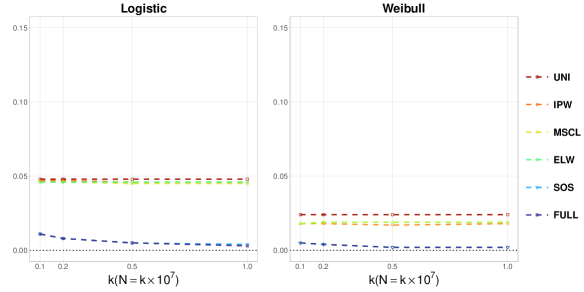
Figure 2 clearly demonstrates that the proposed SOS estimator performs comparably to the full data-based estimator, with the RMSE decreasing as the full data size increases. On the other hand, the RMSE of the UNI, IPW, MSCL, and ELW estimators shows little change as the full data size increases, and remains significantly larger than the RMSE of the SOS estimator.
We also present the bias and SD of above estimators for different full data sizes under the logistic and Weibull models in Tables 3 and 4, respectively.
| FULL | UNI | IPW | MSCL | ELW | SOS | ||||||||
|---|---|---|---|---|---|---|---|---|---|---|---|---|---|
| Bias | SD | Bias | SD | Bias | SD | Bias | SD | Bias | SD | Bias | SD | ||
| 0.1 | 1 | 0.000 | 0.020 | 0.001 | 0.090 | 0.002 | 0.089 | 0.002 | 0.088 | 0.000 | 0.025 | 0.000 | 0.020 |
| 2 | -0.003 | 0.035 | -0.006 | 0.160 | -0.003 | 0.150 | -0.003 | 0.148 | 0.007 | 0.149 | -0.003 | 0.035 | |
| 3 | 0.000 | 0.035 | 0.006 | 0.148 | 0.003 | 0.156 | 0.004 | 0.154 | 0.008 | 0.150 | 0.000 | 0.035 | |
| 4 | -0.001 | 0.036 | -0.001 | 0.162 | -0.007 | 0.154 | -0.006 | 0.152 | 0.000 | 0.146 | -0.002 | 0.036 | |
| 5 | 0.000 | 0.035 | -0.003 | 0.160 | -0.001 | 0.151 | -0.001 | 0.150 | -0.006 | 0.155 | -0.001 | 0.035 | |
| 6 | 0.001 | 0.037 | 0.000 | 0.161 | 0.004 | 0.146 | 0.004 | 0.144 | 0.001 | 0.150 | 0.000 | 0.037 | |
| 7 | 0.001 | 0.034 | -0.002 | 0.162 | 0.001 | 0.152 | 0.001 | 0.149 | 0.002 | 0.156 | 0.000 | 0.034 | |
| 8 | 0.000 | 0.036 | 0.002 | 0.156 | 0.000 | 0.155 | 0.000 | 0.153 | -0.001 | 0.154 | -0.001 | 0.036 | |
| 9 | -0.001 | 0.036 | -0.001 | 0.155 | -0.006 | 0.150 | -0.008 | 0.149 | 0.003 | 0.151 | -0.001 | 0.036 | |
| 10 | 0.002 | 0.036 | 0.006 | 0.160 | -0.013 | 0.156 | -0.012 | 0.154 | 0.009 | 0.154 | 0.001 | 0.036 | |
| 0.2 | |||||||||||||
| 1 | 0.000 | 0.014 | 0.002 | 0.089 | 0.004 | 0.089 | 0.003 | 0.087 | 0.000 | 0.021 | 0.000 | 0.014 | |
| 2 | 0.000 | 0.024 | 0.006 | 0.160 | -0.006 | 0.162 | -0.005 | 0.159 | -0.001 | 0.153 | -0.001 | 0.024 | |
| 3 | -0.001 | 0.025 | 0.003 | 0.154 | 0.001 | 0.152 | 0.001 | 0.149 | 0.001 | 0.151 | -0.001 | 0.025 | |
| 4 | 0.000 | 0.025 | 0.001 | 0.163 | 0.006 | 0.153 | 0.005 | 0.151 | -0.006 | 0.156 | -0.001 | 0.025 | |
| 5 | -0.001 | 0.024 | 0.004 | 0.158 | 0.000 | 0.153 | -0.001 | 0.151 | -0.010 | 0.153 | -0.001 | 0.024 | |
| 6 | 0.000 | 0.025 | 0.002 | 0.154 | 0.006 | 0.152 | 0.005 | 0.151 | -0.002 | 0.152 | 0.000 | 0.025 | |
| 7 | 0.000 | 0.024 | 0.000 | 0.162 | 0.002 | 0.152 | 0.004 | 0.151 | -0.011 | 0.151 | -0.001 | 0.024 | |
| 8 | 0.000 | 0.025 | 0.003 | 0.165 | -0.003 | 0.151 | -0.003 | 0.149 | 0.000 | 0.157 | -0.001 | 0.025 | |
| 9 | 0.000 | 0.025 | -0.004 | 0.157 | -0.002 | 0.153 | -0.002 | 0.150 | 0.000 | 0.155 | 0.000 | 0.025 | |
| 10 | 0.000 | 0.025 | 0.001 | 0.151 | 0.010 | 0.146 | 0.010 | 0.144 | -0.004 | 0.150 | -0.001 | 0.025 | |
| 0.5 | |||||||||||||
| 1 | 0.000 | 0.009 | 0.000 | 0.091 | 0.000 | 0.091 | 0.001 | 0.089 | 0.000 | 0.018 | 0.000 | 0.009 | |
| 2 | 0.001 | 0.015 | 0.007 | 0.159 | -0.003 | 0.148 | -0.003 | 0.147 | -0.001 | 0.151 | 0.001 | 0.015 | |
| 3 | 0.001 | 0.016 | 0.005 | 0.156 | -0.001 | 0.150 | -0.001 | 0.147 | -0.002 | 0.158 | 0.000 | 0.016 | |
| 4 | 0.000 | 0.016 | 0.001 | 0.160 | 0.004 | 0.155 | 0.005 | 0.152 | 0.001 | 0.155 | 0.000 | 0.016 | |
| 5 | 0.000 | 0.015 | 0.005 | 0.155 | 0.002 | 0.147 | 0.001 | 0.146 | -0.002 | 0.156 | -0.001 | 0.016 | |
| 6 | 0.000 | 0.016 | -0.001 | 0.158 | -0.001 | 0.149 | 0.000 | 0.147 | 0.002 | 0.153 | 0.000 | 0.016 | |
| 7 | 0.000 | 0.017 | 0.000 | 0.158 | 0.002 | 0.143 | 0.002 | 0.142 | 0.007 | 0.153 | -0.001 | 0.017 | |
| 8 | 0.000 | 0.016 | -0.010 | 0.158 | 0.005 | 0.145 | 0.006 | 0.142 | 0.007 | 0.149 | -0.001 | 0.016 | |
| 9 | 0.001 | 0.016 | 0.008 | 0.154 | 0.003 | 0.152 | 0.002 | 0.150 | 0.002 | 0.153 | 0.000 | 0.016 | |
| 10 | 0.000 | 0.015 | 0.003 | 0.158 | 0.008 | 0.155 | 0.008 | 0.153 | 0.005 | 0.154 | 0.000 | 0.016 | |
| 1 | |||||||||||||
| 1 | -0.001 | 0.006 | 0.002 | 0.093 | 0.001 | 0.088 | 0.000 | 0.086 | 0.000 | 0.017 | 0.000 | 0.007 | |
| 2 | 0.001 | 0.010 | 0.001 | 0.157 | 0.005 | 0.143 | 0.005 | 0.141 | -0.002 | 0.151 | 0.000 | 0.011 | |
| 3 | 0.002 | 0.011 | 0.003 | 0.159 | -0.003 | 0.153 | -0.004 | 0.149 | -0.002 | 0.158 | 0.000 | 0.012 | |
| 4 | -0.001 | 0.012 | 0.001 | 0.155 | -0.004 | 0.151 | -0.003 | 0.147 | -0.006 | 0.156 | 0.000 | 0.012 | |
| 5 | 0.000 | 0.011 | 0.011 | 0.156 | -0.004 | 0.155 | -0.003 | 0.154 | 0.004 | 0.157 | -0.001 | 0.012 | |
| 6 | 0.000 | 0.011 | -0.002 | 0.160 | -0.005 | 0.145 | -0.005 | 0.144 | 0.000 | 0.150 | -0.001 | 0.011 | |
| 7 | -0.001 | 0.011 | 0.009 | 0.154 | 0.002 | 0.148 | 0.003 | 0.147 | 0.005 | 0.155 | 0.000 | 0.012 | |
| 8 | 0.001 | 0.011 | 0.003 | 0.159 | -0.004 | 0.153 | -0.002 | 0.150 | -0.006 | 0.159 | 0.000 | 0.011 | |
| 9 | 0.001 | 0.010 | 0.006 | 0.157 | 0.004 | 0.147 | 0.004 | 0.145 | 0.000 | 0.149 | 0.000 | 0.011 | |
| 10 | 0.000 | 0.010 | 0.003 | 0.162 | -0.004 | 0.151 | -0.004 | 0.149 | 0.001 | 0.155 | 0.000 | 0.011 | |
| FULL | UNI | IPW | ELW | SOS | |||||||
|---|---|---|---|---|---|---|---|---|---|---|---|
| Bias | SD | Bias | SD | Bias | SD | Bias | SD | Bias | SD | ||
| 0.1 | 1 | 0.000 | 0.004 | 0.000 | 0.017 | 0.000 | 0.018 | 0.000 | 0.013 | -0.001 | 0.004 |
| 2 | 0.000 | 0.010 | 0.000 | 0.047 | 0.000 | 0.041 | 0.000 | 0.034 | -0.001 | 0.010 | |
| 3 | 0.001 | 0.017 | 0.004 | 0.079 | -0.001 | 0.055 | 0.000 | 0.061 | 0.001 | 0.017 | |
| 4 | 0.000 | 0.017 | -0.002 | 0.076 | 0.004 | 0.058 | -0.004 | 0.061 | 0.000 | 0.017 | |
| 5 | 0.000 | 0.018 | 0.000 | 0.080 | -0.001 | 0.059 | 0.002 | 0.060 | 0.000 | 0.018 | |
| 6 | 0.000 | 0.017 | 0.002 | 0.077 | 0.000 | 0.055 | 0.002 | 0.058 | -0.001 | 0.017 | |
| 7 | -0.001 | 0.018 | -0.005 | 0.082 | -0.002 | 0.057 | 0.000 | 0.061 | -0.001 | 0.018 | |
| 8 | -0.001 | 0.017 | 0.002 | 0.080 | -0.002 | 0.056 | -0.002 | 0.059 | -0.001 | 0.017 | |
| 9 | 0.000 | 0.017 | 0.004 | 0.077 | 0.000 | 0.057 | -0.001 | 0.057 | 0.000 | 0.017 | |
| 10 | -0.001 | 0.018 | -0.002 | 0.077 | 0.000 | 0.058 | 0.001 | 0.059 | -0.001 | 0.018 | |
| 11 | -0.001 | 0.017 | -0.001 | 0.078 | 0.002 | 0.057 | 0.003 | 0.062 | -0.001 | 0.017 | |
| 0.2 | |||||||||||
| 1 | 0.000 | 0.003 | 0.001 | 0.018 | 0.001 | 0.017 | 0.000 | 0.013 | -0.001 | 0.003 | |
| 2 | 0.000 | 0.008 | 0.000 | 0.047 | -0.002 | 0.040 | 0.001 | 0.034 | -0.001 | 0.008 | |
| 3 | 0.000 | 0.012 | -0.003 | 0.076 | 0.003 | 0.059 | 0.004 | 0.061 | 0.000 | 0.012 | |
| 4 | 0.001 | 0.013 | 0.001 | 0.077 | 0.001 | 0.058 | -0.002 | 0.059 | 0.000 | 0.013 | |
| 5 | 0.000 | 0.012 | 0.002 | 0.079 | -0.002 | 0.060 | -0.001 | 0.061 | 0.000 | 0.012 | |
| 6 | 0.000 | 0.012 | -0.002 | 0.078 | 0.000 | 0.055 | -0.001 | 0.061 | 0.000 | 0.012 | |
| 7 | 0.000 | 0.013 | 0.001 | 0.078 | -0.001 | 0.059 | -0.002 | 0.063 | 0.000 | 0.013 | |
| 8 | 0.001 | 0.012 | 0.002 | 0.079 | -0.001 | 0.059 | 0.001 | 0.059 | 0.000 | 0.012 | |
| 9 | 0.000 | 0.012 | 0.001 | 0.078 | 0.000 | 0.057 | 0.000 | 0.061 | 0.000 | 0.012 | |
| 10 | 0.000 | 0.012 | 0.003 | 0.077 | 0.001 | 0.056 | 0.000 | 0.059 | -0.001 | 0.012 | |
| 11 | 0.000 | 0.012 | 0.002 | 0.075 | -0.002 | 0.057 | 0.002 | 0.060 | 0.000 | 0.012 | |
| 0.5 | |||||||||||
| 1 | 0.000 | 0.002 | 0.002 | 0.017 | 0.001 | 0.018 | 0.001 | 0.013 | -0.001 | 0.002 | |
| 2 | 0.000 | 0.005 | 0.001 | 0.048 | -0.001 | 0.041 | 0.000 | 0.034 | -0.001 | 0.005 | |
| 3 | -0.001 | 0.008 | -0.002 | 0.075 | 0.002 | 0.057 | 0.002 | 0.061 | -0.001 | 0.008 | |
| 4 | 0.000 | 0.008 | -0.001 | 0.080 | 0.000 | 0.057 | 0.002 | 0.060 | 0.000 | 0.008 | |
| 5 | 0.000 | 0.008 | -0.002 | 0.079 | -0.001 | 0.056 | 0.003 | 0.060 | 0.000 | 0.008 | |
| 6 | 0.000 | 0.008 | 0.001 | 0.077 | 0.002 | 0.056 | -0.001 | 0.062 | 0.000 | 0.008 | |
| 7 | 0.000 | 0.008 | 0.000 | 0.077 | 0.003 | 0.056 | 0.002 | 0.060 | 0.000 | 0.008 | |
| 8 | 0.000 | 0.008 | 0.002 | 0.077 | -0.001 | 0.056 | -0.002 | 0.061 | 0.000 | 0.008 | |
| 9 | 0.000 | 0.008 | 0.004 | 0.079 | 0.001 | 0.054 | -0.001 | 0.059 | 0.000 | 0.008 | |
| 10 | 0.000 | 0.007 | -0.003 | 0.077 | 0.004 | 0.055 | -0.002 | 0.060 | 0.000 | 0.008 | |
| 11 | 0.000 | 0.008 | -0.003 | 0.079 | 0.001 | 0.056 | 0.000 | 0.062 | 0.000 | 0.008 | |
| 1 | |||||||||||
| 1 | 0.000 | 0.001 | 0.001 | 0.017 | 0.001 | 0.018 | 0.000 | 0.013 | -0.001 | 0.001 | |
| 2 | 0.000 | 0.003 | -0.001 | 0.048 | -0.001 | 0.039 | 0.001 | 0.035 | 0.000 | 0.003 | |
| 3 | -0.001 | 0.005 | -0.003 | 0.079 | -0.003 | 0.054 | 0.001 | 0.061 | 0.000 | 0.006 | |
| 4 | -0.001 | 0.006 | 0.000 | 0.078 | 0.002 | 0.057 | 0.000 | 0.063 | -0.001 | 0.006 | |
| 5 | 0.000 | 0.005 | -0.001 | 0.079 | 0.004 | 0.059 | 0.000 | 0.060 | 0.000 | 0.006 | |
| 6 | 0.000 | 0.006 | -0.004 | 0.077 | 0.004 | 0.057 | 0.002 | 0.061 | 0.000 | 0.006 | |
| 7 | 0.000 | 0.006 | 0.004 | 0.077 | 0.004 | 0.057 | 0.001 | 0.059 | 0.000 | 0.006 | |
| 8 | 0.001 | 0.005 | -0.003 | 0.076 | 0.000 | 0.058 | 0.001 | 0.060 | 0.000 | 0.006 | |
| 9 | -0.001 | 0.005 | -0.002 | 0.080 | 0.001 | 0.060 | 0.000 | 0.061 | 0.000 | 0.006 | |
| 10 | -0.001 | 0.005 | -0.001 | 0.077 | 0.001 | 0.057 | 0.001 | 0.059 | -0.001 | 0.006 | |
| 11 | 0.000 | 0.005 | 0.002 | 0.079 | 0.003 | 0.057 | 0.000 | 0.060 | 0.000 | 0.006 | |
Table 3 shows that the bias of all above estimators is similar and small for all full data sizes under the logistic model. The SD of the proposed estimator is similar to that of the full data-based estimator and decreases as the full data size increases. In addition, The SD of the UNI, IPW, MSCL, and ELW subsampling estimators is much larger than that of the proposed estimator, and their SD hardly changes as increases. Under the Weibull model, similar observations as those under the logistic model can be observed from Table 4.
Moving on to the inference performance of the SOS estimator, we calculated the coverage probability of the constructed confidence intervals based on the procedures behind Theorem 1 at a confidence level. The results for different subsample sizes under the logistic and Weibull models are presented in Table 5.
| Logistic | 0.5 | 0.945 | 0.951 | 0.942 | 0.952 | 0.942 | 0.948 | 0.952 | 0.939 | 0.956 | 0.939 | |
|---|---|---|---|---|---|---|---|---|---|---|---|---|
| 1 | 0.949 | 0.955 | 0.945 | 0.952 | 0.951 | 0.947 | 0.954 | 0.939 | 0.948 | 0.945 | ||
| 2 | 0.949 | 0.946 | 0.949 | 0.944 | 0.956 | 0.943 | 0.961 | 0.943 | 0.953 | 0.952 | ||
| 5 | 0.951 | 0.958 | 0.952 | 0.940 | 0.951 | 0.946 | 0.958 | 0.944 | 0.953 | 0.952 | ||
| Weibull | 0.5 | 0.948 | 0.955 | 0.951 | 0.940 | 0.946 | 0.948 | 0.949 | 0.952 | 0.936 | 0.958 | 0.947 |
| 1 | 0.950 | 0.954 | 0.952 | 0.950 | 0.946 | 0.955 | 0.959 | 0.949 | 0.946 | 0.956 | 0.948 | |
| 2 | 0.954 | 0.952 | 0.955 | 0.947 | 0.944 | 0.957 | 0.941 | 0.955 | 0.944 | 0.949 | 0.953 | |
| 5 | 0.955 | 0.953 | 0.956 | 0.942 | 0.945 | 0.958 | 0.949 | 0.957 | 0.944 | 0.947 | 0.949 |
From Table 5, we observe that the proposed SOS estimator achieves satisfactory coverage probabilities close to the nominal level of for both the logistic and Weibull models, regardless of the subsample size . This indicates that the proposed method provides reliable inference for the parameter of interest.
Next, we evaluate the computational performance of the proposed method. All the above estimators are calculated in the R programming (R Core Team, 2016) on a Windows server with a 24-core processor and 128GB RAM. The computing times of these estimators under the logistic and Weibull models for different and are presented in Table 6 and 7 respectively.
| UNI | IPW | MSCL | ELW | SOS | ||
| Logistic | 0.5 | 0.392 | 1.768 | 2.302 | 2.588 | 1.110 |
| 1 | 0.633 | 1.847 | 2.649 | 2.439 | 1.296 | |
| 2 | 0.988 | 2.291 | 3.779 | 2.527 | 1.532 | |
| 5 | 2.953 | 4.948 | 12.792 | 4.798 | 3.522 | |
| FULL: 123.632 seconds | ||||||
| UNI | IPW | ELW | SOS | |||
| Weibull | 0.5 | 1.144 | 2.831 | 3.357 | 1.973 | |
| 1 | 1.887 | 3.676 | 3.816 | 2.630 | ||
| 2 | 3.690 | 5.978 | 5.702 | 4.345 | ||
| 5 | 11.738 | 16.065 | 14.326 | 12.511 | ||
| FULL: 419.887 seconds | ||||||
| FULL | UNI | IPW | MSCL | ELW | SOS | ||
|---|---|---|---|---|---|---|---|
| Logistic | 0.1 | 123.632 | 0.392 | 1.768 | 2.302 | 2.588 | 1.110 |
| 0.2 | 240.100 | 0.633 | 1.847 | 2.649 | 2.439 | 1.296 | |
| 0.5 | 579.839 | 0.988 | 2.291 | 3.779 | 2.527 | 1.532 | |
| 1 | 1088.58 | 2.953 | 4.948 | 12.792 | 4.798 | 3.522 | |
| FULL | UNI | IPW | ELW | SOS | |||
| Weibull | 0.1 | 419.887 | 11.762 | 16.090 | 14.316 | 12.542 | |
| 0.2 | 832.932 | 11.170 | 16.943 | 15.932 | 12.628 | ||
| 0.5 | 2042.820 | 10.433 | 18.245 | 18.029 | 13.377 | ||
| 1 | 3891.762 | 11.134 | 25.554 | 27.281 | 17.134 |
Tables 6 and 7 show that the computing times of the subsampling estimators are significantly shorter compared to the full data-based estimator, particularly evident under the Weibull model and for large full data sizes. This highlights the effectiveness of subsampling methods in reducing the computational burden associated with large-scale datasets. Besides, the computing time of the SOS estimator is comparable to that of the UNI estimator, with the relative difference diminishing as increases. This showcases the computational efficiency of the proposed method.
The SOS method significantly reduces the computational burden while maintaining estimation efficiency compared to the full data-based estimator, emerging as a recommended approach to tackle challenges posed by large-scale data in practical applications.
5 Real data example
In this subsection, we apply the proposed method to a large-scale airline dataset, which is available at http://stat-computing.org/dataexpo/2009/the-data.html. The dataset encompasses flight arrival and departure details for all commercial flights within the United States from October 1987 through April 2008. The full data size is . To analyze the impact of main factors on airline delays, we construct a logistic regression model using the dataset. We uses the arrival delay indicator (1: if the arrival delay is fifteen minutes or more; 0 otherwise) as the response variable. The covariates include day/night, distance from departure to destination, weekend/weekday, and the departure delay indicator (1: if the departure delay is fifteen minutes or more; 0 otherwise). The full data-based estimate of the regression parameter is . The CPU times of calculating the full data-based estimator is seconds. We take the estimation results based on the full data as a reference and then apply the proposed SOS method. We also calculate the UNI, IPW and ELW estimators for comparison. We vary the subsample size to be , , , and . The results calculated based on 200 replicates are presented in Tables 8 and 9.
| UNI | IPW | ELW | SOS | ||||||
|---|---|---|---|---|---|---|---|---|---|
| Bias | SD | Bias | SD | Bias | SD | Bias | SD | ||
| 0.5 | 1 | -0.060 | 1.468 | 0.024 | 0.753 | 0.026 | 0.827 | 0.065 | 0.100 |
| 2 | -0.050 | 1.028 | 0.047 | 0.616 | 0.031 | 0.739 | -0.015 | 0.064 | |
| 3 | 0.055 | 5.139 | -0.194 | 2.483 | -0.356 | 2.589 | 0.068 | 0.399 | |
| 4 | -0.021 | 1.120 | -0.016 | 0.689 | 0.000 | 0.724 | -0.019 | 0.081 | |
| 5 | 0.111 | 1.277 | -0.057 | 0.680 | 0.042 | 0.478 | -0.127 | 0.115 | |
| 1 | |||||||||
| 1 | 0.030 | 1.021 | 0.015 | 0.537 | 0.009 | 0.575 | 0.031 | 0.046 | |
| 2 | -0.045 | 0.689 | 0.019 | 0.444 | 0.024 | 0.489 | -0.008 | 0.029 | |
| 3 | 0.094 | 3.302 | -0.145 | 1.718 | -0.318 | 1.781 | 0.027 | 0.158 | |
| 4 | -0.029 | 0.770 | 0.036 | 0.483 | 0.011 | 0.501 | -0.010 | 0.035 | |
| 5 | 0.025 | 0.912 | -0.079 | 0.459 | 0.053 | 0.336 | -0.056 | 0.048 | |
| 2 | |||||||||
| 1 | -0.038 | 0.689 | 0.013 | 0.391 | 0.030 | 0.403 | 0.015 | 0.023 | |
| 2 | -0.011 | 0.463 | 0.007 | 0.292 | -0.007 | 0.373 | -0.003 | 0.015 | |
| 3 | 0.298 | 2.262 | -0.092 | 1.268 | -0.211 | 1.193 | 0.015 | 0.078 | |
| 4 | -0.017 | 0.545 | 0.024 | 0.348 | -0.008 | 0.345 | -0.005 | 0.017 | |
| 5 | 0.028 | 0.653 | -0.052 | 0.367 | 0.045 | 0.230 | -0.028 | 0.024 | |
| 5 | |||||||||
| 1 | -0.020 | 0.439 | 0.012 | 0.240 | 0.025 | 0.233 | 0.005 | 0.007 | |
| 2 | -0.021 | 0.328 | -0.001 | 0.199 | -0.019 | 0.222 | -0.001 | 0.006 | |
| 3 | 0.230 | 1.443 | -0.005 | 0.769 | -0.015 | 0.720 | 0.008 | 0.031 | |
| 4 | -0.002 | 0.337 | -0.006 | 0.191 | -0.023 | 0.236 | -0.002 | 0.007 | |
| 5 | -0.012 | 0.401 | -0.025 | 0.216 | 0.015 | 0.145 | -0.011 | 0.008 | |
| UNI | IPW | ELW | SOS | |
|---|---|---|---|---|
| 0.5 | 7.008 | 34.26 | 42.406 | 17.624 |
| 1 | 6.815 | 35.485 | 42.494 | 17.041 |
| 2 | 7.130 | 36.138 | 43.870 | 17.625 |
| 5 | 8.066 | 36.339 | 43.590 | 17.974 |
Table 8 provides insights into the performance of different estimators on the airline dataset. The bias of the other subsampling estimators is small, particularly for larger subsample sizes. The standard deviation of the IPW and ELW estimators is smaller than that of the UNI estimator, indicating the effectiveness of designing NSP and incorporating sample moments in improving the estimation efficiency of the UNI method.
However, there is still considerable efficiency loss in these estimators. In contrast, the proposed SOS method outperforms other subsampling estimators in terms of standard deviation. The SD of the proposed method is significantly smaller than that of the IPW and ELW estimators for each component of the parameter of interest, across all subsample sizes. Moreover, the standard deviation decreases at a faster rate as the subsample size increases, indicating the superior efficiency of the proposed method.
Table 9 highlights the computational performance of the estimators. Subsampling methods substantially reduce the computing time compared to the full data-based estimator, with the time of seconds reduced to less than one minute. The UNI method is the fastest among the subsampling estimators. The computing time of SOS estimator is approximately half the time of other subsampling methods. Considering both estimation efficiency and computation efficiency, the results from the numerical studies and real data analyses consistently demonstrate the significant advantages of the proposed SOS method in handling large-scale data.
6 Discussion
This paper proposes the SOS estimator, a simple yet useful subsampling estimator for fast statistical inference with large-scale data. The SOS estimator can achieve a faster convergence rate with the same time complexity as many existing NSP-based subsampling estimators. We obtain the asymptotic distribution of the proposed estimator in the general case with no condition on the ratio between and , and provide a Monte Carlo-based procedure for statistical inference. Extensive numerical results demonstrate the promising finite-sample performance of the SOS estimator.
The current SOS estimator requires the loss function to be smooth. Developing methods to handle non-smooth loss function is a meaningful topic for future research. The SOS estimator is designed for M-estimation problem with a fixed-dimensional parameter. It is of future interest to extend the SOS estimator to general semiparametric estimation problems and problems with high-dimensional parameters.
Acknowledgement
Su’s research was supported by fundamental research funds from the Beijing University of Posts and Telecommunications (No.2023RC47) and the Key Laboratory of Mathematics and Information Networks (Beijing University of Posts and Telecommunications), Ministry of Education, China.
Appendix: proofs for all theoretical results
Lemma S1.
Under Conditions (C1)–(C3), we have
| (6) |
Proof of Lemma S1.
By the definition of , we have
| (7) |
where is between and . Note that by Condition (C1), we have
Since and , then we have by Chebyshev’s inequality, and hence
| (8) |
In addition, under Condition (C2), we can show that
| (9) |
Then (7) together with (8) and (9) implies
| (10) |
By the definition of , we have . Then under Condition (C2), we have . This together with (10) proves under Condition (C3), and hence the result in Lemma S1 is proved.
∎
Proof of Theorem 1.
In the proof, for simplicity of notation, we denote as the kronecker product for any vector . By Taylor’s expansion and some algebras, we have
| (11) |
where and are between and . Note that
By Condition (C1), we have
In addition, under Condition (C2). Then we have
| (12) |
Similarly, under Conditions (C1) and(C2), we can show that
| (13) |
and
| (14) |
Combing (11) – (14), by Lemma S1 and Slutsky’s theorem, we have
| (15) |
Then we have
| (16) |
where is a dimensional random vector sequence with , and is the vectorized form of the upper triangle of
and
| (17) |
with being a symmetrical matrix and the upper triangle matrix of consisting of the elements in arranged in rows.
To prove the result in Theorem 1, according to the continuous mapping in Theorem 2.3 of van der Vaart (2000), it suffices to prove that . Note that can be written as
| (18) |
where and respectively denote the vectorized form and the upper triangle matrix of . Note that . By applying the Lindeber-Feller central limit theorem in Proposition 2.27 in van der Vaart (2000), to prove , it suffices to verify the Lindeberg condition
| (19) |
for every . Since holds for any , then to prove (19), it suffices to prove that
holds for some . By the definition of and Condition (C2), we have . ∎
Proof of Theorem 2.
Similar to Lemma S1, under Conditions (C1)–(C3), we have
| (20) |
Then by the central limit theorem, we have . To prove the results in Theorem 2, it suffices to prove that . Note that
| (21) |
where is between and . For , we have and by Condition (C1) and Chebyshev’s inequality. Then by Condition (C3), we have . In addition, by the definition of and Conditions (C1) and (C2), we have . Then we have .
∎
References
- Ai et al. (2021a) Ai, M., Yu, J., Zhang, H., and Wang, H. (2021a), “Optimal Subsampling Algorithms for Big Data Regressions,” Statistica Sinica, 31, 749–772.
- Ai et al. (2021b) — (2021b), “Optimal subsampling for large-scale quantile regression,” Journal of Complexity, 62.
- Drineas et al. (2006) Drineas, P., Mahoney, M. W., and Muthukrishnan, S. (2006), “Sampling algorithms for regression and applications,” in Proceedings of the seventeenth annual ACM-SIAM symposium on Discrete algorithm, pp. 1127–1136.
- Drineas et al. (2011) Drineas, P., Mahoney, M. W., Muthukrishnan, S., and Sarlós, T. (2011), “Faster least squares approximation,” Numerische Mathematik, 117, 219–249.
- Fan et al. (2022) Fan, Y., Liu, Y., Liu, Y., and Qin, J. (2022), “Nearly optimal capture-recapture sampling and empirical likelihood weighting estimation for M-estimation with big data,” arXiv.
- Fithian and Hastie (2014) Fithian, W. and Hastie, T. (2014), “Local case-control sampling: Efficient subsampling in imbalanced data sets,” The Annals of Statistics, 42, 1693 – 1724.
- Han et al. (2020) Han, L., Tan, K. M., Yang, T., and Zhang, T. (2020), “Local uncertainty sampling for large-scale multiclass logistic regression,” The Annals of Statistics, 48, 1770 – 1788.
- Jordan et al. (2019) Jordan, M. I., Lee, J. D., and Yang, Y. (2019), “Communication-efficient distributed statistical inference,” Journal of the American Statistical Association, 114, 668–681.
- Keret and Gorfine (2023) Keret, N. and Gorfine, M. (2023), “Analyzing big ehr data—optimal cox regression subsampling procedure with rare events,” Journal of the American Statistical Association, 118, 2262–2275.
- Kushilevitz and Nisan (1996) Kushilevitz, E. and Nisan, N. (1996), Communication Complexity, Cambridge University Press.
- Lee et al. (2017) Lee, J. D., Liu, Q., Sun, Y., and Taylor, J. E. (2017), “Communication-efficient Sparse Regression,” The Journal of Machine Learning Research, 18, 1–30.
- Lin and Xi (2011) Lin, N. and Xi, R. (2011), “Aggregated estimating equation estimation,” Statistics and Its Interface, 4, 73–83.
- Luo and Song (2020) Luo, L. and Song, P. X.-K. (2020), “Renewable estimation and incremental inference in generalized linear models with streaming data sets,” Journal of the Royal Statistical Society Series B: Statistical Methodology, 82, 69–97.
- Luo et al. (2023) Luo, L., Wang, J., and Hector, E. C. (2023), “Statistical inference for streamed longitudinal data,” Biometrika, 110, 841–858.
- Ma et al. (2015) Ma, P., Mahoney, M. W., and Yu, B. (2015), “A Statistical Perspective on Algorithmic Leveraging,” Journal of Machine Learning Research, 16, 861–911.
- Ma and Sun (2015) Ma, P. and Sun, X. (2015), “Leveraging for big data regression,” WIREs Computational Statistics, 7, 70–76.
- Mcdonald et al. (2009) Mcdonald, R., Mehryar, M., Nathan, S., Walker, D., and Mann, G. S. (2009), “Efficient Large-Scale Distributed Training of Conditional Maximum Entropy Models,” Advances in Neural Information Processing Systems 22, 1231–1239.
- R Core Team (2016) R Core Team (2016), “A Language and Environment for Statistical Computing,” R Foundation for Statistical Computing, Vienna, Austria. URL https://www.R-project.org.
- Schifano et al. (2016) Schifano, E. D., Wu, J., Wang, C., Yan, J., and Chen, M.-H. (2016), “Online updating of statistical inference in the big data setting,” Technometrics, 58, 393–403.
- Su et al. (2022) Su, M., Wang, R., and Wang, Q. (2022), “A two-stage optimal subsampling estimation for missing data problems with large-scale data,” Computational Statistics & Data Analysis, 173, 107505.
- van der Vaart (2000) van der Vaart, A. W. (2000), Asymptotic Statistics, Cambridge University Press, New York.
- Wang (2019) Wang, H. (2019), “More Efficient Estimation for Logistic Regression with Optimal Subsamples,” Journal of Machine Learning Research, 20, 1–59.
- Wang and Ma (2020) Wang, H. and Ma, Y. (2020), “Optimal subsampling for quantile regression in big data,” Biometrika, 108, 99–112.
- Wang et al. (2019) Wang, H., Yang, M., and Stufken, J. (2019), “Information-Based Optimal Subdata Selection for Big Data Linear Regression,” Journal of the American Statistical Association, 114, 393–405.
- Wang et al. (2018) Wang, H., Zhu, R., and Ma, P. (2018), “Optimal Subsampling for Large Sample Logistic Regression,” Journal of the American Statistical Association, 113, 829–844.
- Wang et al. (2024) Wang, J., Zeng, D., and Lin, D.-Y. (2024), “Fitting the Cox proportional hazards model to big data,” Biometrics, 80, ujae018.
- Yao and Wang (2019) Yao, Y. and Wang, H. (2019), “Optimal subsampling for softmax regression,” Statistical Papers, 60, 585–599.
- Yu et al. (2020) Yu, J., Wang, H., Ai, M., and Zhang, H. (2020), “Optimal Distributed Subsampling for Maximum Quasi-Likelihood Estimators With Massive Data,” Journal of the American Statistical Association, 0, 1–12.
- Zhang et al. (2013) Zhang, Y., Duchi, J. C., and Wainwright, M. J. (2013), “Communication-Efficient Algorithms for Statistical Optimization,” The Journal of Machine Learning Research, 14, 3321–3363.