Kaluza-Klein discreteness of the entropy:

Symmetrical bath and CFT subsystem

Harvendra Singh

Theory Division, Saha Institute of Nuclear Physics

1/AF Bidhannagar, Kolkata 700064, India

Homi Bhabha National Institute (HBNI)

Anushaktinagar, Mumbai 400094, India

Abstract

We explore the entanglement entropy of CFT systems in contact with large bath system, such that the complete system lives on the boundary of $AdS_{d+1}$ spacetime. We are interested in finding the HEE of a bath (system-B) in contact with a central subsystem-A. We assume that the net size of systems A and B together remains fixed while allowing variation in individual sizes. This assumption is simply guided by the conservation laws. It is found that for large bath size the island entropy term are important. However other subleading (icebergs) terms do also contribute to bath entropy. The contributions are generally not separable from each other and all such contributions add together to give rise a fixed quantity. Further when accounted properly all such contributions will form part of higher entropy branch for the bath. Nevertheless the HEE of bath system should be subjected to minimality principle. The quantum minimality principle $S_{quantum}[B]=\{S[A],S_{total}+S[A]\}_{min}$, is local in nature and gives rise to the Page curve. It is shown that the changes in bath entropy do capture Kaluza-Klein discreteness. The minimality principle would be applicable in finite temperature systems as well.

1 Introduction

The AdS/CFT holographic duality [1] has provided a big insight to our understanding of entanglement in strongly coupled quantum theories. Our focus here is on simple cases of the entanglement between two similar type of quantum systems with common interfaces. Generally one believes that sharing of quantum information between systems is guided by unitarity and the locality. Under this principle the understanding of the formation of gravitational black holes like states evolving from a loosely bound pure quantum matter state and the subsequent evaporation process (via Hawking radiation) still remains an unsolved puzzle. Though it is believed that the whole evolution process would be unitary and all information inside the black hole interior (behind the horizon) will be recovered once the black hole fully evaporated. Related to this aspect there is a proposal that the entanglement entropy curve for the bath radiation should bend when the half Page-time is crossed [6]. This certainly is often true when a pure quantum system is divided into two smaller subsystems. But for mixed states of the hawking radiation, or for finite temperature CFTs dual of the AdS-black holes, it is not that straight forward to obtain the Page curve. However, important progress has been made recently in certain models by coupling holographic CFT to an external radiation system (bath), and in some other examples by involving nonperturbative techniques such as wormholes, riplicas and islands [4, 5]. Some answers to the difficult questions have been attempted.

Particularly the AMM proposal for generalized entanglement entropy [4] involves the hypothesis of islandic $(I)$ contribution, and by including gravitational entropy of respective island boundary $(\partial I)$. According to this proposal the ‘quantum’ entropy of a 2-dimensional radiation bath subsystem $(B)$ can be expressed as

$$S_{quantum}[B]=[ext\{{Area(\partial I)\over 4G_{N}}+S[B~{}U~{}I]\}]_{min}$$ (1)

This model uses a hybrid type ‘gravity plus gauge theory’ holographic model. It includes contribution of (gravitational) island entropy to the bath entanglement entropy. The islands are usually disconnected surfaces inside bulk JT gravity. The JT (conformally or nearly AdS) gravity is a dual theory of ‘dot’ like quatum system on the boundary. The same dot lives on the boundary of an infinte $CFT_{2}$ bath system. In the low energy description the JT gravity is treated as a system which is in contact with a 2-dim radiation bath over a flat Minkowski coordinate patch. So there are both field theoretic ($S[B~{}U~{}I]$) as well as gravitational contributions (${Area(\partial I)\over 4G_{N}}$) present in the formula (1). Secondly there is a need to pick the lowest contribution out of a set of many such possible extremas, which may include entropy contributions of islands and the radiation. Although complicated looking, the expression in (1) seemingly reproduces a Page-curve for the bath radiation entropy [4]. However AMM proposal ignores contributions of several subleading terms which we shall altogether pronounce as ’icebergs’ terms. Here it should be clear that the icebergs also are contributions of various disconnected elements to the bath entropy, similar to the islands entropy.

The important feature of AMM-proposal is that it highlights the appearance of island inside bulk gravity. The islands are normally situated outside the black hole horizon. These arise by means of a dynamical principle, and usually the islands are associated with the presence of a bath system when in contact with the quantum-dot. We highlight in present work that other subleading (disconnected) contributions of ‘icebergs’ entropies would have to be properly accounted for in the bath entropy. Here we will be extending our 2-dimensional proposal [18] to the case of higher dimensional CFTs. We provide the picture that no doubt there would exist island contributions but we should not ignore (subleading) icebergs contributions to the bath entropy. If these are ignored we only end up with incomplete interpretation of the Page curve for quantum entropy.

We clearly show that when island, icebergs and leading (pure) bath entropy once added together as a series, that gives rise to a system dependent constant contribution to the entropy of bath system. These contributions are naturally inseparable from each other as they compensate each other perfectly well no matter how large or small their individual contributions could be. We have explicitly shown this phenomenon for limiting case of a quantum dot like system located at the interface of symmetrical CFT bath system [18]. Correspondingly we find that there are gravitational contributions to the bath entropy arising from island and the subleading icebergs, for system-A attached to large bath (subsystem-B). We must note that the entanglement entropy of two such systems together $(AUB)$ can be expanded as

$$S_{total}[AUB]=S_{pure~{}bath}+S_{island}+S_{icebergs}\equiv S_{l}$$

This expansion can always be done whenever system-B is sufficiently large compared to system-A, e.g. see drawing in lower figure in (2).

Figure 1: A symmetrical arrangement of CFT system-A in the center (along $x_{1}$-axis) and CFT bath subsystem-B (of size $b$) situated on either side. The transverse spatial directions other than $x_{1}$ (if any) are all suppressed. The complimentary bath system $(B^{c})$ is also drawn.

Note $S_{l}\gg 0$ is the entropy contained in the total system ($AUB$). It is a constant quantity once the total system size is fixed, and if the system being conserved.

Furthermore, it is proposed that the quantum entropy of entanglement of a large bath subsystem-B should be obtained from local minimality principle

$$S[B]_{quantum}=\{S[A],~{}S_{l}+S[A]\}_{min}=S[A]$$

where $S[A]$ is the entropy of system-A. To make it further clear the above minimality principle works because both $S[A]$ and $S[B]$, as systems being in contact, involve identical local entropies, corresponding to common RT surfaces they do share. Note two systems in contact will have common interfaces fig.(1). The complementary bath system $(B^{c})$ which is semi-infinite on both sides does not play direct role here. For non-contact type systems one should study them separately. In conclusion, the above two equations reproduce the Page curve for the entropy of a large bath system, including for finite temperature systems. The formula is definitely valid at least in static (equillibrium) cases. For time dependent processes involving black hole evaporation, or if there is a continuous change in the total system size (e.g. due to change in mass, energy, or horizon size), the scenario is expected to be similar at any point in time, hence it might be applicable for slow enough processes.

The rest of the article is organized as follows. In section-2 we explain the island and icebergs contributions and define the generalized entropy formulation for pure $AdS$ case. On the boundary we take a finite size system in contact with a symmetrical bath. In section-3 we also discuss a limiting case when system-A becomes very small and appears as point like (where we would use Kaluza-Klein scenario) and is in contact with large size CFT bath. Under Kaluza-Klein perspective the situation emerges similar to that of $2n$ parallel quantum (strip) systems attached to some large bath. The results for the AdS black holes cases are covered in section-4. The section-5 contains a summary.

2 Islands and Icebergs and bath subsystem entropy

Let us consider a system (A) in contact with a bath subsystem (B) in fully symmetrical set up, and both having finite sizes, and living on the boundary of the $AdS_{d+1}$ spacetime. Thus it is assumed that both systems A and B are made of identical field species, i.e. described by same field contents, for simplicity of the problem. The pure $AdS_{d+1}$ spacetime geometry is described by following line element

$$ds^{2}={L^{2}\over z^{2}}(-dt^{2}+dx_{1}^{2}+\cdots+dx_{d-1}^{2}+dz^{2})$$ (2)

where constant $L$ represents a large radius of curvature (in string length units) of spacetime. The coordinate ranges lie $-\infty\leq(t,~{}x_{i})\leq\infty$ and $0\leq z\leq\infty$, where coordinate $z$ represents the holographic range of boundary theory.

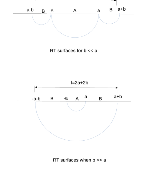
Figure 2: Two different extremal situations are drawn schemetically. The extremal RT surfaces when bath-B size is small compared to the system-A ($b\ll a$), we have all disconnected minimal area surfaces. The lower graph for $b\gg a$ instead has connected surfaces. We keep $l$ same in the both the graphs.

The $CFT_{d}$ theory lives on $d$-dimensional $(t,\vec{x})$ flat Minkowski spacetime describing boundary dynamics of $AdS_{d+1}$ bulk geometry. Consider a set up in which a finite size bath subsystem-B lives on the coordinate patches $[-(b+a),-a]$ & $[a,(b+a)]$ along $x_{d-1}$ direction, whereas system-A, sandwiched in between the bath, lives over the patch $[-a,a]$. The sketches are provided in figures (1), (2) for clarity. The entire systems set-up is arranged in a symmetrical way for the convenience. The states of the system-A and the bath subsystem-B are obviously entangled. The complementary bath system $B^{c}$ lives over the coordinate patches $[b+a,\infty]$ and $[-(b+a),-\infty]$. The $B^{c}$ is semi-infinite on either sides.

From Ryu-Takayanagi holographic prescription the entanglement entropy of a $d$-dimensional $CFT$ strip-shape subsystem of width $l~{}(l=2a+2b)$ is given by

$$S_{total}[AUB]={L^{d-1}V^{(d-2)}\over(2d-4)G_{d+1}}\left({1\over\epsilon^{d-2}}-{b_{0}^{d-1}\over(a+b)^{d-2}}\right)\equiv S_{l}$$ (4)

where $\epsilon\simeq 0$ is the UV cut-off of the $CFT_{d}$ (we shall only consider examples where $d>2$). $V^{(d-2)}$ is the volume of $(d-2)$ spatial directions perpedicular to the strip width direction $x_{1}$. We take $l$ sufficiently large but fixed, so that $S_{l}$ has a constant value. Our aim is to determine entanglement entropy where size $b$ is varied from $b\simeq 0$ to $b\simeq l/2$, by hand. We simply assume local conservation laws, so that the net gain (loss) of system-A is compensated by equal loss (gain) in the size of bath subsystem-B and vice-versa. Note that such a process will keep $l$ fixed. Especially for explicit time dependent cases one may have some definite rate of change, while $\dot{a}=-\dot{b}$ is true due to conservation of energy. The exact rate of loss or gain and the mechanism by which it may happen is not important here and the actual details of the physical process is also not required here. All we are considering is that local conservation laws are at work for complete system within total box size, $l$. Obviously we are assuming here that the system and the bath are made up of identical (CFT) field content. Let us consider two extreme cases below.

Case-1: Independent entropies

When $b\ll a$, for the bath subsystem-B being very small in size, the entanglement entropy of the larger system-A can be found by its extremal surface area as [14, 15]

$$S[A] = {L^{d-1}V^{(d-2)}\over(2d-4)G_{d+1}}\left({1\over\epsilon^{d-2}}-{b_{0}^{d-1}\over a^{d-2}}\right)$$

While the extremal surfaces of bath subsytem on both sides become disconnected. The entropy of small subsystem-B become independently,

$$S[B]={L^{d-1}V^{(d-2)}\over(d-2)G_{d+1}}\left({1\over\epsilon^{d-2}}-{2^{d-2}b_{0}^{d-1}\over b^{d-2}}\right)$$ (6)

Eq.(6) involves area contributions from two disconnected but identical extremal surfaces, which contribute to the bath entropy, see the upper graph as in fig.(2). Note that $S[A]$ and $S[B]$ have the local parts which depend on individual strip parameters $a$ and $b$, respectively, Thus both systems entropies are completely independent even though systems are in contact with each other. The entropy of the small bath system-B would be defined by equation (6) until the crossover point is reached. After the crossover new extremal (connected) surfaces will emerge as drawn in lower graph of fig.(2). We will discuss it next.

Case-2: Entropies with identical local components

When $b\gg a$, in this regime of large bath system the entanglement entropy of system-B is given by the equation

$$S[B]={L^{d-1}V^{(d-2)}\over(2d-4)G_{d+1}}\left({1\over\epsilon^{d-2}}-{2^{d-2}b_{0}^{d-1}\over(l-2b)^{d-2}}\right)+S_{l}$$ (7)

where $S_{l}$ is total entropy of the systems together, which is a fixed quantity. $S_{l}$ gets the contribution from the outer RT surface connecting two farther ends of the symmetrical bath on either side, follow the lower graph in fig(2). Note $S_{l}$ is independent of individual sizes $b$ or $a$, and it is a fixed quantity for given $l$. We might still vary individual system sizes such that we keep $l$ fixed. Now for smaller system-A of strip width $2a$ the entropy is given by

$$S[A]={L^{d-1}V^{(d-2)}\over(2d-4)G_{d+1}}\left({1\over\epsilon^{d-2}}-{2^{d-2}b_{0}^{d-1}\over(l-2b)^{d-2}}\right)$$ (8)

where we have simply used $2a={l}-2b$.

From eqs. (7) and (8), we observe that the $S[A]$ and $S[B]$ differ only by an overall constant, $S_{l}$, otherwise they have the same type of local dependence on $b$. It also implies that under small change in the system sizes

$${\partial S[A]\over\partial b}={\partial S[B]\over\partial b}$$

$${\partial S[A]\over\partial a}={\partial S[B]\over\partial a}$$

Put in other words, $S[A]$ and $S[B]$ represent two independent extrema of the same observable and only differ up to a constant. Classically the areas of these extremal surfaces is such that $S[B]>S[A]$, but quantum entropy of large bath instead would be governed by the minimization

$$S^{quantum}_{b\gg a}[B]=\{S[A],S[A]+S_{l}\}_{min}=S[A]\ .$$ (10)

This states that the quantum entropy of a large bath is the same as the entropy of smaller system-A. Furthermore we note that the quantum entropy of bath decreases as $b$ gets larger and larger but at the same rate as that of system-A. So the Page-curve for entropy of large bath system ($b\gg a$) follows from the principle of minimum entropy, if there exist multiple extrema separated by constants, like $S_{l}$ here. The system-A and the bath subsystem-B entropy otherwise have identical local dependences. This is the net conclusion of the proposal given in eq.(10). Although we might still wonder that the bath entropy ought to have been taken simply as $S[B]$ given in (7), which is net classical area of bulk extremal surface. Instead, as per quantum minimality proposal (10), the bath entropy has to be given by smaller quantity $S[A]$, mainly because both have the same local dependence. The latter is in agreement with the Page curve expectation and unitarity for quantum systems that follows from conservation laws. The quantum entropy proposal shound be taken as complete result for extremal CFTs (at zero temperature) being in contact with symmetrical bath.

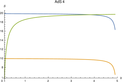
Figure 3: Entropy plots for the values $l=10,~{}\epsilon=.1$, for $CFT_{3}$ system. The lower falling curve (in yellow) is preferable for quantum entropy of large size bath. The rising (green) curve is good for entropy in the small bath region only. The topmost graph is classical entropy of large bath and is not the physical one. We have set ${L^{2}l_{2}\over 2G_{4}}=1$ for the graphs.

Island and Icebergs: full system entropy

We did not explicitly encounter any island like isolated (disconnected) surface area contributions to the entropy so far. So where are these contributions hidden in the above analysis? We have got the Page curve using quantum minimality principle for large bath system without knowing about the island (fragments) entropy contributions. To understand it we need to dissect the total entropy of system-A and system-B. It is vital to understand first what $S[AUB]$ teaches us, even though it is only some system parameter and a fixed quantity. We explore this systematically for $d=3,~{}4$ and $5$ dimensions. (For $d=2$ CFT case, this analysis has been presented in [18].)

i) For $d=3$ CFT: The total system entropy $S_{l}$ is given by ($l=2a+2b$)

$$S_{l}=S[AUB] = {L^{2}l_{2}\over 2G_{4}}\left({1\over\epsilon}-{b_{0}^{2}\over a+b}\right)$$ (11)

where $l_{2}$ is the length of the strip. Making an expansion on the r.h.s. in small ratio $s\ll 1$ $(~{}s={a\over b})$, one can find

$$S_{l} = {L^{2}l_{2}\over 2G_{4}}({1\over\epsilon}-{b_{0}^{2}\over b})+{L^{2}l_{2}\over 2G_{4}}{b_{0}^{2}\over b}(s-s^{2}+s^{3}-\cdots)$$ (12)

$$\equiv S^{(0)}_{bath}+S_{Island}+S_{Icebergs}$$

where expressions in the last line have been identified as: 1) entropy of pure bath:

$$S^{(0)}_{bath}={L^{2}l_{2}\over 2G_{4}}({1\over\epsilon}-{b_{0}^{2}\over b}),~{}~{}~{}~{}~{}$$ (13)

2) subleading gravitational entropy of island-ic boundary:

$$S_{island}={L^{2}l_{2}a\over 2G_{4}}{b_{0}^{2}\over b^{2}},~{}~{}~{}$$ (14)

3) rest all sub-subleading (icebergs) entropies together as:

$$S_{icebergs}=-{L^{2}l_{2}b_{0}^{2}\over 2G_{4}}\left({a^{2}\over b^{3}}-{a^{3}\over b^{4}}+\cdots\right).$$ (15)

Note $S^{(0)}_{bath}$ in eq.(13) represents the HEE of $CFT_{3}$ strip system having width $2b$ (net size of the bath subsystem on both sides). Note it is entropy of pure bath system without the presence of system-A. Whereas $S_{island}$, which genuinely represents the interactions between bath-B and system-A, is the ‘gravitational’ entropy of island-like boundary situated at $z=b$ (e.g. corresponding to an island-like region lying in between $z=\infty$ and $z=b$ inside the $AdS_{4}$). The codim-2 island boundary located at $z=b$ has a geometrical area:

$${\cal{A}}_{island}={2L^{2}l_{2}a\over b^{2}}$$

It is proportional to actual size $2l_{2}a$ of boundary CFT system-A. Thus geometric entropy of island eq.(14) may be expressed as

$$S_{island}={{\cal{A}}_{island}\over 4\tilde{G}_{4}}$$

Here $\tilde{G}_{4}=G_{4}/b_{0}^{2}$ is treated as effective Newton’s constant. Other sub-subleading terms, which are altogether named as icebergs’ entropies, include contributions from remaining terms in small $s$ expansion. Thus by doing a series expansion it gets revealed that the various terms in the series (12) although may have got distinct interpretations, but they are actually inseparable from each other. No matter what these individual values might be, all the terms are important because these add up nicely to constitute $S_{l}$, i.e. the total entropy. The total entropy, including island and icebergs, thus has a constant value, for given $l$. (The $S_{l}$ depends only on the parameter $l$, which is measure of total systems size. In this sense $S_{l}$ is actually a global quantity.) One could still vary $a$ and $b$ individually but keeping $l(=2a+2b)$ fixed. That means the bath size could grow at the cost of size of system-A and vice versa, under mutual local exchanges or those processes which may lead to shift in the mutual interface of systems A and B. (This appears akin to what might happen in black hole evoparation processes also, e.g. through Hawking radiation, where the Hawking radiation is treated as bath.) Perhaps simple CFT models may teach us something about the black hole evoparation process! The relevant entropy graphs are plotted in the figure (3) with a discussion in the caption for small and large bath cases.

Unitarity and the locality of entropy

The question still arises what would happen if we ignored the subleading (icebergs) contributions in eq.(12), due to their smallness, as being subleading $O(s^{2})$ and even smaller. Although one is free to do so but we immediately find that the r.h.s. of $S_{l}$ will now start depending on $a$ and $b$ in independent ways! This will lead to varied conclusions regarding the Page curve, unitarity and about the information content of the systems. Alternatively we may decide that $S_{icebergs}$ terms should not be dropped from leading terms in any situation. In other words precise knowledge of isolated contributions is vital for the unitarity! Furthermore, the island and the icebergs would remain invisible, as these contribute to eq. (7), which is an higher entropy extrema and hence unphysical as per ‘quantum entropy’ proposal of bath-B. The latter reason solely arises from the quantum entropy principle that for large size bath entropy should be taken with smaller value amongst $(S_{l}+S[A])$ and $S[A]$, where $S_{l}\gg 0$ is total entropy.

ii) $d=4$ case: For $CFT_{4}$ the total system entropy $S[AUB]$ can be written as

$$S_{l} = {L^{3}l_{3}l_{2}\over 4G_{5}}\left({1\over\epsilon^{2}}-{b_{0}^{3}\over(a+b)^{2}}\right)$$ (16)

where $l_{2}\&l_{3}$ are the sizes of two transverse spatial coordinates of the $CFT_{4}$ on the boundary of $AdS_{5}$ geometry. The systems are separated along $x_{1}$ direction. By making an expansion on the r.h.s. in (16), for small $s$ we get

$$S_{l} = {L^{3}l_{3}l_{2}\over 4G_{5}}\left({1\over\epsilon^{2}}-{b_{0}^{3}\over b^{2}}+{b_{0}^{3}\over b^{2}}s(1+s)^{-2}\right)$$ (17)

$$= {L^{3}l_{3}l_{2}\over 4G_{5}}\left({1\over\epsilon^{2}}-{b_{0}^{3}\over b^{2}}+{b_{0}^{3}\over b^{2}}(s-2s^{2}+O(s^{3}))\right)$$

$$\equiv S^{(0)}_{B}+S_{Island}+S_{Icebergs}$$

where break up of various expressions in the last line is as: the leading pure bath entropy,

$$S^{(0)}_{B}={L^{3}l_{3}l_{2}\over 4G_{5}}({1\over\epsilon^{2}}-{b_{0}^{3}\over b^{2}}),~{}~{}~{}~{}~{}$$ (18)

the island-ic (gravitational) entropy,

$$S_{island}={L^{3}l_{3}l_{2}b_{0}^{3}a\over 4G_{5}b^{3}}\equiv{{\cal{A}}_{island}\over 4\tilde{G}_{5}},~{}~{}~{}$$ (19)

and other subleading icebergs entropies:

$$S_{icebergs}=-{L^{3}b_{0}^{3}l_{3}l_{2}\over 2G_{5}}\big{[}{a^{2}\over b^{4}}-{a^{3}\over 3b^{5}}+\cdots\big{]}.$$ (20)

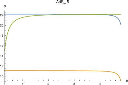
Figure 5: Entropy plots for the values $l=10,~{}\epsilon=.3$, for the $CFT_{4}$ system. The lower falling curve (yellow) is only preferred for quantum entropy at large $b$. The rising (green) curve is good only for bath entropy in small $b$ region only. The topmost graph is classical entropy for large bath but it is unphysical. We have set ${L^{3}l_{3}l_{2}\over 4G_{5}}=1$.

Note again $S_{island}$ is proportional to ${2L^{3}l_{3}l_{2}a\over b^{3}}$ which is the geometrical area of extended 3-dim island boundary located at $z=b$ inside $AdS_{5}$ spacetime, with a redefined 5-dim Newton’s constant as $\tilde{G}_{5}=G_{5}/b_{0}^{3}$. The related entropies are plotted in the figure (5). They exhibit similar properties as $d=3$ case for small and large bath cases.

iii) For $d=5$ case: Above results clearly tell us that for $CFT_{5}$ the subsystem entanglement properties would also be similar to $d=3,~{}4$ cases. We may convince ourselves that it will be a common occuring phenomenon whenever there are two systems (system and the bath) in contact, i.e. separated by interfaces. The islands and icebergs typically arise as a result of interactions and information sharing between the dofs of the systems.

3 Lower dimensional Kaluza-Klein perspective: Multiple thin strips

Figure 4: An arrangement of system-A (in the middle on $x_{1}$-axis) and CFT bath subsystem-B of size $b$ each lie on either side. All transverse spatial directions (if any) except $x_{1}$ direction are suppressed. The complimentary bath system $(B^{c})$ is also drawn.

It is important to discuss special case of the systems described by eq.(7). Consider very small size for system-A, such that $a\simeq R$, where $R$ is Kaluza-Klein scale of the theory (analogous to JT-gravity and near $CFT_{1}$ case). (We expect that for such small size system, with a narrow width, system-A could be effectively treated as being compactified on $S^{1}$, with a compactification radius $R$, but $R\gg\epsilon$.) In that case we can safely take $a\simeq\pi nR$, with $n$ being a positive integer. For simplificity we shall consider only small $n$ values, also $\epsilon\ll\pi R\ll b$ (If there is any difficulty one can simply take $n=1$). The system-A can essentially be treated as assembly of $2n$ narrow (parallel) strips sandwiched between symmetrical bath system-B (on either sides of total size $2b$). We have a situation as depicted in the figure (4), where transverse directions $x_{2}$ and $x_{3}$ are suppressed. An expansion on the r.h.s of (7), for small ${n\ll{b\over\pi R}}$, gives bath entanglement entropy (for $d=3$)

$$S[B] =S_{l}+{L^{2}l_{2}\over 2G_{4}}({1\over\epsilon}-{b_{0}^{2}\over n\pi R})$$ (21)

$$\equiv(S^{(0)}_{bath}+S_{island}+S_{icebergs})+S_{2n-strips}[R]$$

where leading term $S^{(0)}_{bath}$ is same as described earlier, and other expressions are

$$S_{island}={L^{2}l_{2}\over 4G_{3}}{n\over b^{2}},~{}~{}~{}$$

$$S_{icebergs}=-{L^{2}l_{2}\over 4G_{3}}({n^{2}\pi Rb_{0}^{2}\over b^{3}})+O(n^{3})$$ (22)

The $G_{3}=G_{4}/(2\pi R)$ is 3-dimensional Newton’s constant. The islandic contribution, especially for $n=1$, is similar to the gravitational entropy of the island boundary situated at $z=b$ inside bulk. The $S_{icebergs}$ includes rest all subleading contributions. The eq.(21) involves an infinite series which is perturbative. Actually it will not be wise to separate icebergs from first two leading terms in (21) at all! They all remain important as the total sum of these terms (within the parenthesis) sum up to $l$-dependent entropy $S_{l}$. It is quite clear from the starting line of the perturbative expansion in (21).

While the entanglement entropy of the $2n$ parallel strips, assembled side by side, and in contact with bath, is simply (for $d=3$)

$$S_{2n-strips}[A]={L^{2}l_{2}\over 2G_{4}}({1\over\epsilon}-{b_{0}^{2}\over n\pi R})$$ (23)

and the bath system entropy is

$$S[B]=S_{l}+S_{2n-strips}[R]$$ (24)

The local $R$-dependent terms in eqs. (23) and (24) are identical, and since the two expressions differ only by an overall constant $S_{l}$, the actual ‘quantum entropy’ of bath would be given by the local entropy contained in system-A (multiple narrow strips) only. So under minimality selection rule quantum entropy of bath should simply be stated as

$$S^{quantum}[B]=\{S_{2n-strips},S_{l}+S_{2n-strips}\}_{min}=S_{2n-strips}$$ (25)

where entopy of all $2n$ parallel strips arranged together is given above. Note $l_{2}$ is length of these strips, and the individual strip width is taken as $\pi R$. This is the net entanglement entropy of a large bath system, when $b\gg R$, i.e. towards the end of the Page curve. It entirely gets its contribution from single RT surface homologous to central $2n$ strips system. Note the narrow strips have width $\pi R$ $(\ll b)$. It is important to note that the bath entropy is discretized since KK-level $n$ takes integral values ($n\in Z$). Obviously we would trust these results for small $n$ values only. For large $n$ it would be good to use noncompact continuum description in one higher dimensions.

It can be concluded that the entropy for a large bath will necessarily show discrete jumps as and when KK level changes. This is an example of strongly coupled system of $2n$ parallel sheets (system-A) placed in the middle of large symmetrical CFT baths on either side. The conclusions shall remain unchanged even under infinite size limit $(b\to\infty,~{}l\to\infty)$ and thus should be treated universal. We conclude that we would not be able to see island and icebergs physically, as their net contribution to entropy always results in a fixed constant only.

3.1 Entropy spectrum of strip systems

We are interested in exchanging small number of strips between bath (B) and the multi-strip system (A). This will lead to changes in the systems entanglement entropy. Note a small number of strip exchanges between B and A will not change the total entropy $S_{l}$. Thus net change in entropy of system-A with KK-strips number $n_{2}$ and with KK-strips number $n_{1}$ can be found to be $(n_{1}<n_{2})$

$$\bigtriangleup S_{1\to 2} =S_{strips}[n_{2}]-S_{strips}[n_{1}]$$ (26)

$$={L^{2}l_{2}\over 2G_{4}}({1\over n_{1}}-{1\over n_{2}}){b_{0}^{2}\over\pi R}$$

$$\equiv{1\over T_{E}}\bigtriangleup E_{1\to 2}$$

In the last line the entanglement temperature of bath can be taken as $T_{E}\simeq{1\over l}$ [16]. Empirically we may determine that typical change in energy density of systems (energy per unit strip-length)

$${\bigtriangleup{\cal E}_{1\to 2}}={\bigtriangleup E_{1\to 2}\over l_{2}}={L^{2}b_{0}^{2}\over 2\pi G_{4}lR}({1\over n_{1}}-{1\over n_{2}})={L^{2}b_{0}^{2}\over 4\pi^{2}G_{3}lR^{2}}({1\over n_{1}}-{1\over n_{2}})$$ (27)

This energy spectrum is obviously discrete in nature! A fixed quantum of energy exchanges is required to take place between bath-B and multi-strip system-A during an exchange of the strips. Note we are discussing the CFT ground state (zero temperature) only. The spectrum appears analogous to the atomic spectrum, but system-A here is made up of discrete number of strips whereas a finite number of strips (quantum matter and not the photons) are exchanged between various KK levels. This exchange process entails KK-level ‘jumps’. Here $n_{1}=1$ may be treated as the lowest level (for smallest size single strip system) while $n_{2}>1$ will correspond to higher levels (more than one strip cases). Note a level jump in the strip number is necessarily associated with discrete (quantum) CFT matter exchanges between system and its surrounding bath. The relevant physical scale is compactification radius $R$.

A plausible interpretation of above energy spectrum may be given as follows. The discrete KK modes have typical momentum $\sim{1\over R}$. (The strip length $l_{2}$ is some large quantity (fixed), $L\gg 1$ is $AdS$ radius of curvature, $G_{3}\equiv G_{4}/(2\pi R)$ is 3-dim Newton’s constant.) Thus

$$\bigtriangleup E_{1\to 2}\propto{1\over R^{2}}$$

appears primerily due to the KK momentum modes in this case. The energy-matter exchanges between central strip system-A and the bath are precise and discrete! We emphasize that with more careful analysis of subleading terms in the entropy, we might be able to see winding modes contributions! We hope to report about it in subsequent communications.

A similar analysis for 4-dimensional $CFT_{4}$ would provide energy density in exchanges

$${\bigtriangleup E_{1\to 2}\over l_{3}l_{2}}={L^{3}b_{0}^{3}\over 8\pi^{3}G_{4}lR^{3}}({1\over n_{1}^{2}}-{1\over n_{2}^{2}})$$ (28)

where $(l_{3}l_{2})$ is the transverse size of the $3d$ strips, where the individual width of strips is $\sim\pi R$.

We will show that change in entanglement entropy under strip exchange (or KK level jumps) can be determined for finite temperature cases as well. There the $|\bigtriangleup E|$ will involve thermal corrections. Perturbatively we shall estimate and find that the leading thermal correction grows proportional to $R$, the width of the strips. We guess these corrections involve string winding modes.

4 Finite temperature systems

The previous exercise can be extended to the case of CFT at finite temperature as well. The whole process goes in parallel for any CFT system which is in a mixed state. The limitation is that for $d>2$ case the HEE at finite temperature can only be estimated by using perturbative methods. Alternative options would be resort to the numerical approach. Consider the asymptotically $AdS_{d+1}$ geometry that has Schwarzschild black hole at the center

$$ds^{2}={L^{2}\over z^{2}}(-f(z)dt^{2}+{dz^{2}\over f(z)}+dx_{1}^{2}+\cdots+dx_{d-1}^{2})$$ (29)

where $f(z)=(1-{z^{d}\over z_{0}^{d}})$ with $z=z_{0}$ being the location of black hole horizon. There is a finite temperature in the field theory on AdS boundary. Assume now that the strip shaped system-A with strip width $2a$ is taken in thermal equillibrium with symmetrical bath system-B on either sides, so that system-A is located in the middle of bath (net width of bath system being $2b$). Other transverse directions of the systems are infinitely extended. Here both systems $A$ and $B$ have same temperatures. We only discuss the case when $a\ll b$, because $a\gg b$ case is rather straight forward. The entanglement entropy of the strip like bath system-B on the boundary of (29) can be written as

$$S[B]=S_{l}({l,z_{0}})+S({2a,z_{0}})=S_{l}({l,z_{0}})+S({l-2b,z_{0}})$$ (30)

In our notation a functional $S(x,z_{0})$ represents the HEE for strip system having width $x$ obtained from area of extremal surfaces in a black-brane AdS geometry [17]. The $z_{0}$ dependences indicate there is finite temperature effect (horizon dependence). Note the first term on the r.h.s. of (30) involves those constants which treat system-A and bath-B together as single entity. It measures a global information involving $A$ and $B$. Only second term has the local entropy information regarding central system-A like the size and location of interface boundaries between system-A and bath-B.

Usually for small width $x$ one can estimate $S({x,z_{0}})$ using perturbative tools as discussed in [17]. It is the best method so long as we have $x\ll z_{0}$. Also this is what one would be requiring most when approaching the end of the Page curve involving two systems A & B. Typically the perturbative series looks like [17]

$$S({x,z_{0}})=S_{0}(x)+S_{1}(x,z_{0})+S_{2}(x,z_{0})+\cdots$$ (31)

where leading term $S_{0}(x)$ is the entropy of AdS ground state, see eqs.(2) and (6), while the first order term is given by

$$S_{1}({x,z_{0}})={L^{d-1}V^{(d-2)}\over 16G_{d+1}}{(d-1)a_{1}x^{2}\over(d+1)b_{0}^{2}z_{0}^{d}}$$ (32)

note it has explicit horizon $(z_{0})$ dependence, and same is true for second order term and so on. (Here $a_{1}$ and $b_{0}$ are specific dimension dependent coefficients involving explicit Beta-functions, see appendix of [17]).

At the same time the entanglement entropy of central system-A, having width $2a$, is given by

$$S[A]=S({2a,z_{0}})=S({l-2b,z_{0}})$$ (33)

In second equality we used $l=2a+2b$, as the bath has size $2b$. Again one can compare that the expressions in equations (30) and (33) differ only by an over all constant (global) quantity $S_{l}({l,z_{0}})$, that depends only on full size (system plus symmetrical bath) $l$. From the perspective of system-A $S_{l}$ is some global fixed quantity. Therefore we conclude that these two equations represent two different extrema of the same entropy observable, primerily because both entropies contain identical local terms. The local terms arise from extremal RT surface that connects common interfaces of systems A and B. These local terms contain mutual entanglement information which two systems share between them. Further eqs. (30) and (33) are telling us that they contain identical entanglement entropy (through local exchanges along common interfaces) for system $A$ and system $B$. Classically they differ only up to overall constant. We conclude that ‘quantum’ entanglement entropy measure at finite temperature for large bath subsystem-B (i.e. $b\gg a$) ought to be taken as the smaller value between (30) and (33). Therefore the quantum entropy of any large thermal bath system (in contact with smaller system-A) would be

$$S_{quantum}[B]=\{S[A],S_{l}+S[A],\cdots\}_{min}=S[A]\ .$$ (34)

The above result in (34) is consistent with the expectations of the quantum entropy Page curve when bath is very large. Note this conclusion is independent of how large $l$ might be, so long as $b\gg a$ is obeyed! In infinite bath limit $b\to\infty$ ( $l\to\infty$, $a=fixed$), the constant $S_{l}$ has a limit:

$$S_{l}(l,z_{0})\to S_{BH}(z_{0})$$

where $S_{BH}$ is black hole entropy. So we will get

$$\lim_{b\to\infty}S_{quantum}[B]=\{S[A],S_{BH}+S[A],\cdots\}_{min}\equiv S[A]=S(2a,z_{0})\ .$$ (35)

The right hand side of the eqs. (34) and (35) are identical. Hence for mixed states irrespective of the overall system size, the entropy of a large bath system is determined by the entropy of smaller system-A, under quantum minimality principle. $S[A]$ again accounts for the smallest entanglement entropy between two contact systems A & B, even in thermal case!

Perhaps an interesting stage (during blackhole evaporation) can arise when system-A size becomes very small such that it becomes comparable to intermediate Kaluza-Klein scale of the theory, i.e. $a\simeq n\pi R$, and $b\simeq{l\over 2}-\pi nR$, where $R$ is radius of Kaluza-Klein circle. Then bath entropy may be expressed as

$$S_{quantum}[B]=S({2\pi nR,z_{0}})$$ (36)

which is the entropy of $2n$ independent strips (or sheets) put together. It is the smallest quantum entropy for a large bath, and is quantized by the virtue of the presence of KK scale in the (bulk) theory. However we should trust this result for small $n\in Z$ values only. It is clear that any change in large bath entropy tends to be discrete in nature, if there exists KK scale. Similarly, one can deduce that during quantum evolution of a black hole state after long times, i.e. towards the end of evaporation, when system-A will shrink to zero size, the bath entropy

$$S_{quantum}[B]\to 0\ .$$

That means all the information which was kept within system-A has been transferred to system-B (a very large bath). No loss of information can be expected in this process even for thermal systems!

4.1 Spectrum of narrow KK strips

When the size of the system-A becomes very small such that it is closer to a Kaluza-Klein radius, $R$, we can set system size as $2a\simeq 2n\pi R$, for some integer KK-level $n\geq 1$. ($n=0$ means there is no system-A.) We are now interested in exchang of a small number of KK strips between bath (B) and the strip system (A). We may call this process as ‘sheets of CFT matter’ exchange between bath and system-A at their mutual interfaces. This will result in change of level $n$ for the system-A. The resulting change in entanglement entropy from level $n_{2}$ to $n_{1}$ can be calculated $(n_{1}<n_{2})$ as

$$\bigtriangleup S_{1\to 2} =S_{strips}[n_{2}]-S_{strips}[n_{1}]$$ (37)

$$={L^{2}l_{2}\over 2G_{4}}({1\over n_{1}}-{1\over n_{2}}){1\over\pi R}+\bigtriangleup S_{thermal}$$

$$\equiv{1\over T_{E}}\bigtriangleup E_{1\to 2}$$

Assuming entanglement temperature can be set as $T_{E}={1\over l}$. So empirically it can be determined that change in energy of strips is discrete,

$${\bigtriangleup E_{1\to 2}}={L^{2}l_{2}\over G_{3}l(2\pi R)^{2}}({1\over n_{1}}-{1\over n_{2}})+{\bigtriangleup E_{1\to 2}^{thermal}}$$ (38)

A conclusion is drawn from here that a discrete quantum of energy would have to be exchanged between outer bath system-B and central (strip-like) system-A for finite temperature CFT. The length of strips $l_{2}$ is some large value (fixed), $L\gg 1$ is AdS radius of curvature, and $G_{3}$ is the Newton’s constant.

The thermal part of entropy is difficult to estimate exactly. However in the regime of our interest, when $a\ll z_{0}$, we can evaluate it perturbatively. From (32) up to first order (say, for the $CFT_{3}$)

$$\bigtriangleup E_{1\to 2}^{thermal}={L^{2}l_{2}\over 32G_{3}l}{a_{1}\pi(n_{2}^{2}-n_{1}^{2})R\over 2b_{0}^{2}z_{0}^{3}}$$ (39)

Thus schematically we get

$$|\bigtriangleup E_{1\to 2}|\propto{1\over n_{1}n_{2}R^{2}}+\#{(n_{2}+n_{1})R\over z_{0}^{3}}$$

Indeed the first term appears primerily due to the KK momentum modes. While the second term (due to thermal correction) grows linearly with $R$, which we guess presumably is consequence of string winding (wrapping) modes. We conclude that these energy and matter exchanges are all discrete! The same analysis can also be done for other $CFT_{d}$.

5 Summary

We have proposed that quantum entropy of entanglement for a large bath system-B (CFT) when in contact with small subsystem-A follows quantum minimality principle

$$S_{quantum}[B]=\{S[A],S[A]+S_{l},\cdots\}_{min}=S[A].$$

where $S_{l}$ is full system $(AUB)$ entropy. Any small fluctuation in the size of system-A (due to the matter exchange with bath) would not alter this conclusion provided systems follow conservation laws. Thus the equation realizes the Page curve for the entropy of quantum matter in contact with sufficiently large bath system. This conclusion is based upon the observation that for small subsystem-A and relatively large bath-B the respective entanglement entropies differ only by an overall constant. The constant does depend on the total systems size $(l)$, which is fixed. For this reason $S_{l}$ is conserved and quantum information it contains is essentially global.

We have explicitly shown that islands and subleading entropis (icebergs) contribute to the unphysical extremum of bath entropy. Actually all these contributions form various parts of $S_{l}$ only. The (physical) quantum entropy of bath however does not get contribution from these fictitious parts! In this light the entropy expression (1) is very close to our proposal, but it is only approximate and may not cover full account of quantum entanglement between systems, mainly it ignores vital subleading contributions beyond the islands. On the contrary, we have shown that there will be an infinitum of such subleading contributions. It is shown to be true for all $CFT_{d}$ systems in equillibrium. Furthermore we have analysed our results when subsystem-A size becomes ‘point-like’, similar in size as Kaluza-Klein scale of the theory, if there exist such an scale. As the small system size approaches KK-scale, we find necessary discreteness in the entropy and the energy spectrum due to existence of low lying KK towers. Should there be no spontaneous compactification scale in the theory, the entropy of a large bath would vanish smoothly as and when the subsystem-A disappears. In summary it is indicated that the change in bath entropy does capture Kaluza-Klein discreteness.

Acknowledgments: It is pleasure to thank Stefan Theisen for several insightful discussions on this subject. I am thankful to MPI Golm for the kind hospitality where part of this work was carried out. The financial support from the Alexander-von-Humboldt foundation is also highly acknowledged.

Appendix A An effective construction of the hybrid gravity and CFT systems

For small size central CFT subsystem-A, such that its size $2a\approx 2\pi R$, i.e. when the system size can approximately fit within the Kaluza-Klein radius, the system-A may be treated as being point like. The symmetrical bath subsystem-B on either side is being comparatively very large so it can continue to be described by respective (noncompact) CFT. However, for all practical purposes, with out any loss of physical picture, the system-A can also be replaced by dual ‘near AdS’ geometry in one lower spacetime dimensions. The Newton’s constant for near-AdS bulk geometry would become $G_{d}=G_{d+1}/(2\pi R)$. We have tried to draw these situations in the figure (6) for systems $A$, $B$ and the compliment system $B^{c}$. The mixed gravity and CFT systems set up has been a favourable arrangement for an island proposal [4].

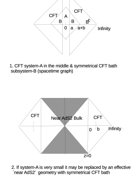
Figure 6: An hybrid arrangement of the gravitational and CFT systems.

References

- [1] J. Maldacena, Adv. Theor. Math. Phys. 2, 231 (1998) arXiv:9711200[hep-th]; S. Gubser, I. Klebanov and A.M. Polyakov, Phys. lett. B 428, 105 (1998) arXiv:9802109[hep-th]; E. Witten, Adv. Theor. Math. Phys. 2, 253 (1998) arXiv:9802150[hep-th].
- [2] A.K. Pati and S.L. Braunstein, NATURE 404, 164 (2000); S.L. Braunstein and A.K. Pati, Phys. Rev. Lett. 98, 080502 (2007).
- [3] J. R. Samal, A. K. Pati, and Anil Kumar, Phys. Rev. Lett. 106, 080401 (2011).
- [4] A. Almheiri, R. Mahajan and J. Maldacena, “Islands outside the horizon”, arXiv:1910.11077[hep-th].
- [5] G. Penington, S. H. Shenker, D. Stanford and Z. Yang, “Replica wormholes and the black hole interior”, arXiv:1911.11977[hep-th]; A. Almheiri, T. Hartman, J. Maldacena, E. Shaghoulian and A. Tajdini, “Replica Wormholes and the Entropy of Hawking Radiation”, JHEP05 (2020) 013, arXiv:1911.12333.
- [6] D. N. Page, “Average entropy of a subsystem”, Phys. Rev. Lett. 71 (1993) 1291–1294, [gr-qc/9305007].
- [7] S. Raju, “Lessons from the Information Paradox”, arXiv:2012.05770.
- [8] L. Susskind, arXiv:1810.11563[hep-th]; Fortschr. Phys. 64 (2016) 24; D. Stanford and L. Susskind, Phys. Rev. D90 (2014) 126007.
- [9] A.R. Brown , D.A. Robert, L. Susskind, B. Swingle, and Y. Zhao, Phys. Rev. Lett 116 (2016) 191301; A.R. Brown , D.A. Robert, L. Susskind, B. Swingle, and Y. Zhao, Phys. Rev. Lett 93 (2016) 086006;
- [10] A. Bernamonti et.al, Phys. Rev. Lett. 123 (2019) 081601.
- [11] K. Hashimoto, N. Iizuka, and S. Sugishita, Phys. Rev D96 (2017) 126001; K. Hashimoto, N. Iizuka, and S. Sugishita, arXiv:1805.04226[hep-th]
- [12] R. Jackiw, ”Lower Dimensional Gravity”, Nucl. Phys. B252, 343 (1985).
- [13] C. Teitelboim, ” Gravitational and Hamiltonian Structure in Two Space-Time Dimensions”, Phys. Lett. 126B, 41 (1983).
- [14] S. Ryu and T. Takayanagi, Phys. Rev. Lett. 86 (2006) 181602, arXiv:0603001[hep-th]; S. Ryu and T. Takayanagi, ”Aspects of Holographic Entanglement Entropy”, JHEP 0608 (2006) 045, arXiv:0605073[hep-th].
- [15] V. Hubeny, M. Rangamani and T. Takayanagi, JHEP 0707 (2007) 062, arXiv: 0705.0016 [hep-th].
- [16] Jyotirmoy Bhattacharya, Masahiro Nozaki, Tadashi Takayanagi, and Tomonori Ugajin Phys. Rev. Lett. 110, 091602.
- [17] R. Mishra and H. Singh, JHEP 10 (2015) 129, e-Print:1507.03836 [hep-th]; S. Maulik and H. Singh, JHEP 04 (2021) 065, e-Print: 2012.09530 [hep-th]
- [18] H. Singh, ”Islands and Icebergs may contribute nothing to the Page curve”, e-Print: 2210.13970 [hep-th]