Constrained Approximate Optimal Transport Maps

Abstract

We investigate finding a map $g$ within a function class $G$ that minimises an Optimal Transport (OT) cost between a target measure $\nu$ and the image by $g$ of a source measure $\mu$. This is relevant when an OT map from $\mu$ to $\nu$ does not exist or does not satisfy the desired constraints of $G$. We address existence and uniqueness for generic subclasses of $L$-Lipschitz functions, including gradients of (strongly) convex functions and typical Neural Networks. We explore a variant that approaches a transport plan, showing equivalence to a map problem in some cases. For the squared Euclidean cost, we propose alternating minimisation over a transport plan $\pi$ and map $g$, with the optimisation over $g$ being the $L^{2}$ projection on $G$ of the barycentric mapping $\overline{\pi}$. In dimension one, this global problem equates the $L^{2}$ projection of $\overline{\pi^{*}}$ onto $G$ for an OT plan $\pi^{*}$ between $\mu$ and $\nu$, but this does not extend to higher dimensions. We introduce a simple kernel method to find $g$ within a Reproducing Kernel Hilbert Space in the discrete case. Finally, we present numerical methods for $L$-Lipschitz gradients of $\ell$-strongly convex potentials.

1 Introduction

Let $\mu$ and $\nu$ denote two probability distributions on two (potentially different) measurable spaces $\mathcal{X}$ and $\mathcal{Y}$. Many problems in applied fields can be written under the form

$$\underset{g\in G}{\inf}\ \mathcal{D}(g\#\mu,\nu),$$ (1)

where $\#$ denotes the push-forward operation, $\mathcal{D}$ is a non-negative discrepancy (such as a distance metric or a $\phi$-divergence) measuring the similarity between $g\#\mu$ and $\nu$, and $G$ is a set of acceptable functions between $\mathcal{X}$ and $\mathcal{Y}$. Under appropriate assumptions on $\mathcal{D}$, this problem can be interpreted as a projection of $\nu$ on the set $G\#\mu:=\{g\#\mu,g\in G\}$ for the discrepancy $\mathcal{D}$. In this paper, we focus on cases where $\nu$ cannot be written as $g\#\mu$ for $g\in G$.

One prominent example of Eq. 1 within machine learning and applied statistics is model inference. If $\nu$ is a discrete distribution of data samples, the goal is to infer the adequate parameter $\theta$ of a parametric model $\{\mu_{\theta},\;\theta\in\Theta\}$ such that $\mu_{\theta}$ fits $\nu$ as well as possible. This can be done by maximum likelihood, but also by minimising a well-chosen discrepancy between $\mu_{\theta}$ and $\nu$. In the highly popular field of generative modelling, the parametric model $\mu_{\theta}$ is written $g_{\theta}\#\mu$, with a latent distribution $\mu$, often taking the form of a Gaussian distribution in $\mathbb{R}^{k}$ or a uniform distribution over a hypercube, and a set of parametric functions $G=\{g_{\theta},\;\theta\in\Theta\}$ represented by a specific neural network architecture. The discrepancy $\mathcal{D}$ is often chosen as the Kullback-Leibler divergence [20] or the Wasserstein distance [4]. In such problems, it is clear that we do not target $g\#\mu=\nu$, since it would mean that the model has only learned to reproduce existing samples, and not to create new ones. This is possible because the expressivity of neural networks is limited, but also because the training steps usually impose regularity properties on $g$ and constrain its Lipschitz constant in order to increase its robustness [37, 18] or stabilise its training [25].

In an Euclidean setting, another example of Eq. 1 appears when we need to compare two distributions $\mu$ and $\nu$ potentially living in spaces of different dimensions, or when some invariance to some geometric transformations is required (for problems such as shape matching or word embedding). In such cases, it is usual to choose $G$ as a well chosen set of linear or affine embeddings (such as matrices in the Stiefel manifold if the space dimension is different between $\mathcal{X}$ and $\mathcal{Y}$). For instance, this idea underpins several sets of works introducing global invariances in optimal transport [2, 31].

In both of the previous examples, $G$ is parametrised by a set $\Theta$ of parameters which is potentially extremely large (for neural networks) but of finite dimension. Alternatively, the set of functions $G$ can be much more complex and characterised by regularity or convexity assumptions, the problem becoming non-parametric. This is typically the case in the field of optimal transport [36, 32]. Given $\mu$ and $\nu$ probability measures on respective Polish spaces $\mathcal{X}$ and $\mathcal{Y}$, Monge’s Optimal Transport consists in finding a Transport map $T$ such that $T\#\mu=\nu$ and which minimises a given displacement cost. When there is no map $T$ such that $T\#\mu=\nu$ (for example, if $\mu$ is discrete and if $\nu$ is not), or when the map solution does not meet the regularity requirements for some given practical application, it makes sense instead to solve problems of the form of Eq. 1, with $\mathcal{D}$ a Wasserstein distance and $G$ a set of functions with acceptable regularity. For instance, as studied in [26], $G$ can be composed of functions $g=\nabla\phi$ with $\phi$ $\ell$-strongly-convex with an $L$-Lipschitz gradient. For cases where $\mu$ is discrete, this formulation also overcomes a classic shortcoming of numerical optimal transport approaches, which usually compute solutions which are only defined on the support of $\mu$. If a machine learning algorithm requires the computation of the transport of new inputs, the map must be either recomputed, or an approximation of the previous map must be defined outside of the support of $\mu$. Several solutions have been proposed in the literature to solve this problem [10, 6, 22, 26, 28], and some of them [22, 26] consists in solving Eq. 1 with an appropriate set of functions $G$. Consistency and asymptotic properties of such estimators are also the subject of several of these works [10, 22, 21].

OT discrepancies. In this paper, we focus on problems of the form Eq. 1 when $\mathcal{D}$ is chosen as an optimal transport discrepancy for a general ground cost $c$. We recall that if $\mathcal{X}$ and $\mathcal{Y}$ are two Polish spaces, the Optimal Transport cost between two measures $\nu_{1}\in\mathcal{P}(\mathcal{X})$ and $\nu_{2}\in\mathcal{P}(\mathcal{Y})$ for a ground cost function $c:\mathcal{X}\times\mathcal{Y}\longrightarrow\mathbb{R}_{+}$ is defined by the following optimisation problem

$$\mathcal{T}_{c}(\nu_{1},\nu_{2})=\underset{\pi\in\Pi(\nu_{1},\nu_{2})}{\min}\ \int_{\mathcal{X}\times\mathcal{Y}}c(x,y)\mathrm{d}\pi(x,y),$$ (2)

where $\Pi(\nu_{1},\nu_{2})$ is the set of probability measures on $\mathcal{X}\times\mathcal{Y}$ whose first marginal is $\nu_{1}$ and second marginal is $\nu_{2}$. Given this method of quantifying the discrepancy between $g\#\mu$ and $\nu$, Eq. 1 becomes

$$\underset{g\in G}{\inf}\ \mathcal{T}_{c}(g\#\mu,\nu).$$ (3)

In the case where the source measure is discrete and the target measure is absolutely continuous, the Optimal Transport problem in Eq. 3 is said to be semi-discrete, and has a slightly more explicit expression (see [24] for a course on the matter). If we suppose in addition that $c(x,y)=\|x-y\|_{2}^{2}$ and that the source measure weights are uniform ($a_{i}=1/n$), then Eq. 3 is a constrained version the Optimal Uniform Quantization problem studied thoroughly in [23].

Existence of minimisers. An important question regarding this optimisation problem concerns the existence of minimisers, depending on the ground cost $c$ and the set of functions $G$. While numerous works in the literature have focused on the convergence of optimisation algorithms (such as stochastic gradient descent) to critical points for this kind of problem [17], the existence of minimisers has surprisingly been little studied. We derive in Theorems 2.5 and 2.6 generic conditions to ensure existence of such minimisers in $G$, and show counter-examples when these conditions are not met. We also show that these conditions are satisfied for two classes of functions, namely classes of $L$-Lipschitz functions which can be written as gradient of $l$-strongly convex functions (recovering a result shown in [26] as a particular case of Theorem 2.6), and classes of neural networks with Lipschitz activation functions. We also discuss uniqueness of the solutions, which is usually not satisfied, and remains a difficult question without strong assumptions on the set of functions $G$.

Approximating a coupling. In the field of optimal transport, a particular setting where Eq. 3 is interesting is when we have access to a non deterministic coupling $\pi$ solution of a regularised version of a optimal transport between two probability measures $\mu$ and $\nu$. For instance, the entropic optimal transport [27], or the mixture Wasserstein formulation [12] both yield optimal plans $\pi$ which cannot be trivially written as optimal maps between $\mu$ and $\nu$. For some applications, it can be interesting to approximate $\pi$ by another transport plan supported by the graph of a function with possible additional regularity assumptions. This can be done by approximating $\pi$ by $(I,g)\#\mu$, with specific regularity properties on $g$, which is a particular case of Eq. 3, replacing $\nu$ by $\pi$ and $G$ by the set $H:=\{(I,g),g\in G\}$. In this specific setting, we show in Section 2.7 under which conditions on the ground cost $c$ the solutions of this problem between plans are equivalent to solutions of the original Eq. 3 when $\pi\in\Pi(\mu,\nu)$.

Alternate minimisation. Under appropriate assumptions, Eq. 3 can be rewritten as a minimisation problem over $\pi\in\Pi(\mu,\nu)$ and $g\in G$:

$$\underset{g\in G}{\min}\ \underset{\pi\in\Pi(\mu,\nu)}{\min}\ \int_{\mathcal{X}\times\mathcal{Y}}c(g(x),y)\mathrm{d}\pi(x,y).$$ (4)

This naturally leads to consider Eq. 3 as an alternate minimisation problem, that we study in Section 3 in the Euclidean case when $c(x,y)=\|x-y\|_{2}^{2}$. More precisely, we show that  Eq. 3 is strongly linked to the barycentric projection problem: when $\pi$ is fixed, the solution $g$ minimising Eq. 4 can be reinterpreted as the $L^{2}$-projection of the barycentric projection of $\pi$ on the set $G$. In the one-dimensional case, when $G$ is a subclass of increasing functions, this yields an explicit solution to the problem (as it was shown in [26] in a more specific case), and we show that this explicit solution does not hold in dimension larger than $1$ by presenting a counter-example.

Outline of the paper. In this work, we address problem Eq. 1 for large classes of functions $G$. In Section 2, we define the problem and establish general conditions for the existence of solutions, exploring examples involving gradients of convex functions and neural networks. Section 3 examines the link between Eq. 1 and a constrained barycentric projection problem, demonstrating an explicit solution in one dimension and providing a counterexample in higher dimension. Section 4 focuses on practical numerical methods to solve the optimisation problem, with a particular emphasis on classes within a Reproducing Kernel Hilbert Space, and the case of gradients of strongly convex functions.

2 A Constrained Approximate Transport Map Problem

2.1 Problem Definition

We consider $(\mathcal{X},d_{\mathcal{X}})$ a locally compact Polish space, and $\mu\in\mathcal{P}(\mathcal{X})$ a probability measure on $\mathcal{X}$. Our objective is to find a map $g:\mathcal{X}\longrightarrow\mathbb{R}^{d}$ verifying the constraint $g\in G$ for some class of functions $G\subset(\mathbb{R}^{d})^{\mathcal{X}}$, such that the image measure $g\#\mu$ is "close" to a fixed probability measure $\nu\in\mathcal{P}(\mathbb{R}^{d})$, in the sense of Eq. 3.

Applying the definition of $\mathcal{T}_{c}$ directly (Eq. 2) yields the following expression for Eq. 3:

$$\underset{g\in G}{\inf}\ \underset{\pi\in\Pi(g\#\mu,\nu)}{\min}\ \int_{\mathcal{X}\times\mathbb{R}^{d}}c(x,y)\mathrm{d}\pi(x,y).$$ (5)

The optimisation variable $g$ acts on the set of constraints of the Optimal Transport problem, however thanks to a well-known "change of variables" result ([14] Lemmas 1 and 2 for a reference), we will be able to reformulate Eq. 5. In the following, we shall denote by $\Pi_{c}^{*}(\nu_{1},\nu_{2})$ the set of minimisers of the optimal transport problem Eq. 2 between two measures $\nu_{1}$ and $\nu_{2}$.

Lemma 2.1.

([14], Lemmas 1 and 2) Let $\mathcal{X},\mathcal{Y},\mathcal{X}^{\prime},\mathcal{Y}^{\prime}$ Polish spaces. Let $g:\mathcal{X}\longrightarrow\mathcal{X}^{\prime}$ and $h:\mathcal{Y}\longrightarrow\mathcal{Y}^{\prime}$ two measurable maps and let $(\mu,\nu)\in\mathcal{P}(\mathcal{X})\times\mathcal{P}(\mathcal{Y})$. Consider two costs $c:\mathcal{X}\times\mathcal{Y}\longrightarrow\mathbb{R}$ and $c^{\prime}:\mathcal{X}^{\prime}\times\mathcal{Y}^{\prime}\longrightarrow\mathbb{R}$ such that $\forall(x,y)\in\mathcal{X}\times\mathcal{Y},\;c(x,y)=c^{\prime}(g(x),h(y))$.

• For any $\gamma^{\prime}\in\Pi(g\#\mu,h\#\nu)$, there exists $\gamma\in\Pi(\mu,\nu)$ such that $\gamma^{\prime}=(g,h)\#\gamma$.

• We have $\Pi_{c^{\prime}}^{*}(g\#\mu,h\#\nu)=(g,h)\#\Pi_{c}^{*}(\mu,\nu)$.

Using Lemma 2.1, the energy of the map problem Eq. 3 can be written as follows:

$$\mathcal{T}_{c}(g\#\mu,\gamma)=\underset{\pi\in\Pi(\mu,\nu)}{\inf}\ \int_{\mathcal{X}\times\mathbb{R}^{d}}c(g(x),y)\mathrm{d}\pi(x,y).$$ (6)

In our study of the map problem Eq. 3, we will consider classes $G$ that are a subset of the $L$-Lipschitz functions. The first reason is that with unbounded Lipschitz constants, the problem may not have a solution, as we shall see in Section 2.5. Moreover, there are multiple practical considerations that lead to choosing functions with an upper-bounded Lipschitz constant. To begin with, numerous practical models enforce this condition, such as Wasserstein GANs [4], and diffusion models [33] (see also [30] Appendix S2), furthermore most neural networks are Lipschitz (since typical non-linearities are chosen as Lipschitz), and the control of the Lipschitz constant may be desirable as a regularisation method [37]. From a theoretical standpoint, a Lipschitz function $g$ has the convenient property of conserving the moment conditions of a measure $\mu$ through its image measure, as we show in Lemma 2.2, which automatically ensures the finiteness of the transport cost $\mathcal{T}_{c}(g\#\mu,\nu)$ for measures admitting $p$-moments and $c(x,y)=d_{\mathcal{X}}(x,y)^{p}$.

Lemma 2.2.

Let $(\mathcal{X},d_{\mathcal{X}})$ a Polish space and $\mu$ a probability measure on $\mathcal{X}$ with a finite moment of order $p\geq 1:$ $\int_{\mathcal{X}}d_{\mathcal{X}}(x_{0},\cdot)^{p}\mathrm{d}\mu<+\infty$ (for any or all $x_{0}\in\mathcal{X}$). Then for an $L$-Lipschitz function $g:\mathcal{X}\longrightarrow\mathcal{Y}$, with $(\mathcal{Y},d_{\mathcal{Y}})$ a Polish space, the push-forward measure $g\#\mu$ also has a finite moment of order $p$.

Proof.

Choose $y_{0}\in\mathcal{Y}$ and $x_{0}\in\operatorname{supp}(\mu)$. We have $\int_{\mathcal{Y}}d_{\mathcal{Y}}(y_{0},y)^{p}\mathrm{d}g\#\mu(y)=\int_{\mathcal{X}}d_{\mathcal{Y}}(y_{0},g(x))^{p}\mathrm{d}\mu(x)$, then given $x\in\mathcal{X}$, write

$$d_{\mathcal{Y}}(y_{0},g(x))^{p} \leq(d_{\mathcal{Y}}(y_{0},g(x_{0}))+d_{\mathcal{Y}}(g(x_{0}),g(x)))^{p}$$

$$\leq 2^{p-1}(d_{\mathcal{Y}}(y_{0},g(x_{0}))^{p}+d_{\mathcal{Y}}(g(x_{0}),g(x))^{p})$$

$$\leq 2^{p-1}(d_{\mathcal{Y}}(y_{0},g(x_{0}))^{p}+2^{p-1}L^{p}d_{\mathcal{X}}(x_{0},x)^{p},$$

where we used the inequality $(a+b)^{p}=2^{p}(\frac{a}{2}+\frac{b}{2})^{p}\leq 2^{p-1}(a^{p}+b^{p})$ for $a,b\geq 0$, by convexity of $t\longmapsto t^{p}$. Now the constant $2^{p-1}d_{\mathcal{Y}}(y_{0},g(x_{0}))^{p}$ is $\mu$-integrable since $\mu$ is a probability measure, and the function $d_{\mathcal{X}}(x_{0},\cdot)^{p}$ is integrable since $\mu$ has a finite moment of order $p$. ∎

For the sake of legibility, we focus on the case where the target space is $\mathbb{R}^{d}$, however it is possible to extend our considerations to a target space $\mathcal{Y}$ which is a Polish space verifying the Heine-Borel property (i.e. that any bounded and closed set is a compact set), which in particular allows the case where $\mathcal{Y}$ is a connected and complete smooth Riemannian manifold (in which case the Heine-Borel property follows from the Hopf-Rinow Theorem, see [13] Theorem 2.8). Similarly, the problem naturally extends to the case where the codomain of the maps $g$ and the target measure $\nu$ are different spaces $\mathcal{Y},\mathcal{Y}^{\prime}$.

In Fig. 1, we illustrate a solution of the map problem using numerical methods introduced in Section 4.2, for two different values of $L$ (the Lipschitz constant of the maps $g$).

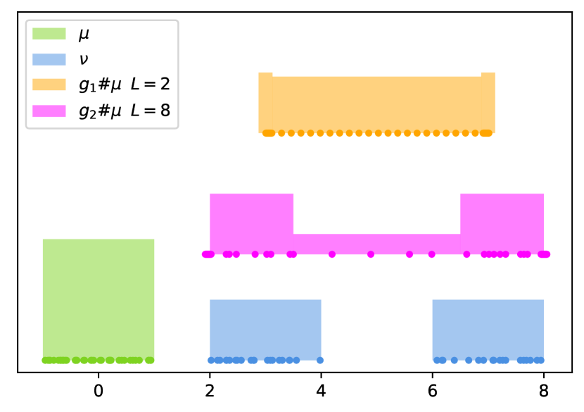
(a) Illustration of the source, target and image measures using their samples and (approximate) densities.

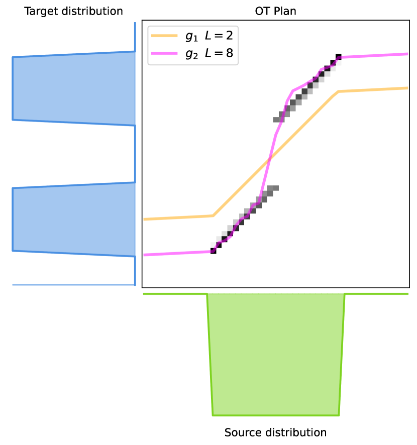
(b) Illustration of map solutions and comparison with the (discontinuous) Optimal Transport coupling.

Figure 1: Illustration of solutions of maps problems (Eq. 3) on a toy dataset with a source measure $\mu=\mathcal{U}([-1,1])$ and a target measure $\nu=\frac{1}{2}\mathcal{U}([2,4])+\frac{1}{2}\mathcal{U}([6,8])$. The two solutions are respectively $L=2$ and $L=8$ Lipschitz.

2.2 Existence of a Solution

To formulate an existence result, we shall apply the direct method of calculus of variations, for which we require the following technical lemma, which states that the Optimal Transport cost $\mathcal{T}_{c}$ is lower-semi-continuous with respect to the weak convergence of measures.

Lemma 2.3.

Let $c:\mathcal{Y}\times\mathcal{Y}^{\prime}\longrightarrow\mathbb{R}_{+}$ a lower-semi-continuous cost function, and $(\mu_{n})_{n\in\mathbb{N}}\in\mathcal{P}(\mathcal{Y}){N}$ and $(\nu)_{n\in\mathbb{N}}\in\mathcal{P}(\mathcal{Y}^{\prime}){N}$ such that $\forall n\in\mathbb{N},\;\mathcal{T}_{c}(\mu_{n},\nu_{n})<+\infty$.

Assume that $\mu_{n}\xrightarrow[n\longrightarrow+\infty]{w}\mu\in\mathcal{P}(\mathcal{Y})$ and $\nu_{n}\xrightarrow[n\longrightarrow+\infty]{w}\nu\in\mathcal{P}(\mathcal{Y}^{\prime})$. Then:

$$\underset{n\longrightarrow+\infty}{\liminf}\mathcal{T}_{c}(\mu_{n},\nu_{n})\geq\mathcal{T}_{c}(\mu,\nu).$$

Proof.

Using the Kantorovich duality formulation in [32] Theorem 1.42, we see that $\mathcal{T}_{c}(\mu,\nu)$ is a supremum of lower-semi-continuous functions, hence also a lower-semi-continuous function of $(\mu,\nu)$ (see  [32] Box 1.5). ∎

In order to state a general existence result, we introduce a condition on the class of functions $G$.

Definition 2.4.

We say that a set of functions $G\subset(\mathbb{R}^{d})^{\mathcal{X}}$ is stable by local uniform limit if there exists a sequence $(\mathcal{K}_{m})$ of compact sets of $\mathcal{X}$ verifying $\cup_{m}\mathcal{K}_{m}=\mathcal{X}$ such that:

for any sequence $(g_{n})_{n\in\mathbb{N}}\in G{N}$ such that for all $m$, $(g_{n}|_{\mathcal{K}_{m}})_{n\in\mathbb{N}}$ converges uniformly towards a function $g_{\mathcal{K}_{m}}:\mathcal{K}_{m}\longrightarrow\mathbb{R}^{d}$, there exists $g\in G$ such that $g|_{\mathcal{K}_{m}}=g_{\mathcal{K}_{m}}$ for all $m$.

Theorem 2.5.

Let $c:\mathbb{R}^{d}\times\mathbb{R}^{d}\longrightarrow\mathbb{R}_{+}$ a continuous cost function, a probability measure $\mu\in\mathcal{P}(\mathcal{X})$ on a locally compact Polish space $(\mathcal{X},d_{X})$, and $\nu\in\mathcal{P}(\mathbb{R}^{d})$. If:

• (Coercive cost). There exists $y_{0}\in\mathbb{R}^{d}$ such that $c(y,y_{0})\xrightarrow[\|y\|_{2}\longrightarrow+\infty]{}+\infty$;

• (Locally Lipschitz cost). For all $y\in\mathbb{R}^{d},\;$ and for any compact set $\mathcal{K}\subset\mathbb{R}^{d}$, $c(\cdot,y)$ is $\kappa_{y,\mathcal{K}}$-Lipschitz on $\mathcal{K}$, with $\int\kappa_{y,\mathcal{K}}\mathrm{d}\nu(y)<+\infty$;

• (Local uniform stability of $G$). $G$ is a subset of the space of $L$-Lipschitz functions from $\mathcal{X}$ to $\mathbb{R}^{d}$, that is stable by local uniform limit (see Definition 2.4);

• (Problem finiteness) There exists $g\in G$ such that $\mathcal{T}_{c}(g\#\mu,\nu)<+\infty$;

then the problem $\underset{g\in G}{\operatorname{argmin}}\ \mathcal{T}_{c}(g\#\mu,\nu)$ has a solution.

Proof.

— Step 1: Defining a minimising sequence.

We introduce the notation $J(g):=\mathcal{T}_{c}(g\#\mu,\nu)$ for convenience, and $J^{*}$ the problem value, which is finite by Assumption iv). Consider a minimising sequence $(g_{n})_{n\in\mathbb{N}}\in G{N}$ such that

$$\forall n\in\mathbb{N},\;J(g_{n})\leq J^{*}+2^{-n}.$$

— Step 2: Bounding $g_{n}$.

First, we fix $n\in\mathbb{N}$, a compact set $A\subset\mathcal{X}$ of diameter $r>0$ such that $\mu(A)>0$, and $a\in A$. We lower-bound:

$$J(g_{n})\geq\underset{\pi\in\Pi(\mu,\nu)}{\min}\int_{A\times\mathbb{R}^{d}}c(g_{n}(x),y)\mathrm{d}\pi(x,y).$$

Now for $(x,y)\in A\times\mathbb{R}^{d}$, we lower-bound

$$c(g_{n}(x),y) =\left|c(g_{n}(a),y)-\left(c(g_{n}(a),y)-c(g_{n}(x),y)\right)\right|$$

$$\geq c(g_{n}(a),y)-\left|c(g_{n}(a),y)-c(g_{n}(x),y)\right|$$

$$\geq c(g_{n}(a),y)-\kappa(y)\|g_{n}(a)-g_{n}(x)\|_{2}$$

$$\geq c(g_{n}(a),y)-\kappa(y)Ld_{\mathcal{X}}(a,x)$$

$$\geq c(g_{n}(a),y)-\kappa(y)Lr,$$

where we defined $\kappa(y):=\kappa_{y,g_{n}(A)}$ and used Assumptions ii) and iii). We introduce the constant $K:=-Lr\int\kappa\mathrm{d}\nu$, which does not depend on $n$. Our previous computations yield the lower-bound

$$J(g_{n})\geq\int_{\mathbb{R}^{d}}c(g_{n}(a),y)\mathrm{d}\nu(y)+K,$$

where we used the marginal constraints on the variable $\pi\in\Pi(\mu,\nu)$. We now fix $y_{0}\in\mathbb{R}^{d}$ and $s>0$ such that $\nu(\overline{B}(y_{0},s))>0$, and continue to lower-bound

$$J(g_{n}) \geq\int_{\overline{B}(y_{0},s)}c(g_{n}(a),y)\mathrm{d}\nu(y)+K$$

$$\geq\nu(\overline{B}(y_{0},s))\ \underset{y\in\overline{B}(y_{0},s)}{\min}\ c(g_{n}(a),y)+K$$

$$\geq\nu(\overline{B}(y_{0},s))\ c(g_{n}(a),y^{*})+K,$$

where the continuity of $c(g_{n}(a),\cdot)$ allowed to choose a minimiser $y^{*}\in\overline{B}(y_{0},s)$. We now use Assumption i), the inequality

$$\nu(\overline{B}(y_{0},s))\ c(g_{n}(a),y^{*})+K\leq J^{*}+1$$

shows that there exists a constant $M$ independent on $n$ such that $\|g_{n}(a)\|_{2}\leq M$. Indeed, if it were the case that $\|g_{n}(a)\|_{2}\xrightarrow[n\longrightarrow+\infty]{}+\infty$, then Assumption i) would contradict the inequality above, for $n$ large enough.

— Step 3: Applying Arzelà-Ascoli’s Theorem on a compact subset of $\mathcal{X}$.

Since $G$ is stable by local uniform limit (see Definition 2.4), we can choose $(\mathcal{K}_{m})_{m\in\mathbb{N}}$ compact sets of $\mathcal{X}$ associated to uniform local stability on $G$. We can suppose that the sequence $(\mathcal{K}_{m})$ is increasing for the inclusion, and contains $a$ (introduced in Step 2). For $m\in\mathbb{N}$, we use the upper-bound from Step 2 and the fact that each $g_{n}$ is $L$-Lipschitz:

$$\forall x\in\mathcal{K}_{m},\;\|g_{n}(x)\|_{2}\leq M+L\underset{y\in\mathcal{K}_{m}}{\max}\ d_{\mathcal{X}}(y,a),$$

which shows that the sequence $(g_{n})$ is uniformly bounded on $\mathcal{K}_{m}$. The sequence $(g_{n})$ is equi-Lipschitz and thus equi-continuous on the compact set $\mathcal{K}_{m}$, thus by Arzelà-Ascoli’s theorem, we can choose $\alpha_{m}:\mathbb{N}\longrightarrow\mathbb{N}$ an extraction such that $g_{\alpha_{m}(n)}\xrightarrow[n\longrightarrow+\infty]{}g_{m}$ uniformly on $\mathcal{K}_{m}$, for a certain function $g_{m}\in\mathcal{C}^{0}(\mathcal{K}_{m},\mathbb{R}^{d})$.

— Step 4: Diagonal extraction to prove subsequential convergence of $(g_{n})$ on $\mathcal{X}$

Without loss of generality, we assume that the extractions $(\alpha_{m})$ from Step 3 are such that for $m<m^{\prime}$, $\alpha_{m^{\prime}}$ is a sub-extraction of $\alpha_{m}$. Consider the diagonal extraction $\beta:n\longmapsto\alpha_{n}(n)$. By construction, the sequence $(g_{\beta(n)})$ converges uniformly towards $g_{m}$ on each $\mathcal{K}_{m}$. By assumption (Definition 2.4), there exists $g\in G$ such that $g|_{\mathcal{K}_{m}}=g_{\mathcal{K}_{m}}$ for each $m\in\mathbb{N}$. Furthermore, we have the convergence $g_{\beta(n)}\xrightarrow[n\longrightarrow+\infty]{}g$ uniformly on each $\mathcal{K}_{m}$, thus we have $g_{\beta(n)}\xrightarrow[n\longrightarrow+\infty]{}g$ uniformly on all compact sets of $\mathcal{X}$.

— Step 5: Showing that the limit $g$ is optimal

First, by the dominated convergence theorem, given the convergence from Step 4, the sequence $g_{\beta(n)}\#\mu$ converges weakly towards the probability measure $g\#\mu$. This allows us to apply Lemma 2.3, which provides the following inequality:

$$\underset{n\longrightarrow+\infty}{\liminf}J(g_{\beta(n)})\geq J(g),$$

where $J$ was introduced in Step 1, where we also chose $g_{n}$ such as $J(g_{n})\leq J^{*}+2^{-n}$, thus we conclude $J^{*}\geq J(g)$, hence $g$ is optimal.

∎

Theorem 2.5 can be extended to the case where the regularity of the functions of $G$ is only assumed on a partition of $\mathcal{X}$.

Theorem 2.6.

Let $c:\mathbb{R}^{d}\times\mathbb{R}^{d}\longrightarrow\mathbb{R}_{+}$ a continuous cost function, a probability measure $\mu\in\mathcal{P}(\mathcal{X})$ on a locally compact Polish space $(\mathcal{X},d_{\mathcal{X}})$, and $\nu\in\mathcal{P}(\mathbb{R}^{d})$. Consider $(E_{i})_{\llbracket 1,K\rrbracket}$ a partition of $\mathcal{X}$ such that for every $i\in\llbracket 1,K\rrbracket,\;\mu(\partial E_{i})=0$. Under the same conditions as Theorem 2.5, and replacing assumption iii) by

• The class of functions $G\subset(\mathbb{R}^{d})^{\mathcal{X}}$ is of the form

  $$G=\left\{g:\mathcal{X}\longrightarrow\mathbb{R}^{d}\ |\ \forall i\in\llbracket 1,K\rrbracket,\;g|_{\mathring{E_{i}}}=g_{i},\;g_{i}\in G_{i}\right\},$$

  where for every $i\in\llbracket 1,K\rrbracket$, the set of functions $G_{i}\subset(\mathbb{R}^{d})^{\mathring{E_{i}}}$ is a subset of the space of $L$-Lipschitz functions from $\mathring{E_{i}}$ to $\mathbb{R}^{d}$, that is stable by local uniform limit (see Definition 2.4),

then the problem $\underset{g\in G}{\operatorname{argmin}}\ \mathcal{T}_{c}(g\#\mu,\nu)$ has a solution.

Proof.

We shall follow closely the proof of Theorem 2.5, and point out the technical differences. We introduce a minimising sequence exactly identically to Step 1. The computations from Step 2 can be done verbatim, choosing instead a compact set $A_{i}\subset\mathring{E_{i}}$, and concluding $\|g_{n}(a_{i})\|_{2}\leq M_{i}$ for a fixed $a_{i}\in A_{i}$.

Steps 3 and 4 are then done separately on each $\mathring{E_{i}}$, yielding extractions $(\beta_{i})$ such that each $g_{\beta(i)}$ converges locally uniformly on $\mathring{E_{i}}$ towards a function $g_{i}\in G_{i}$. Considering the extraction $\beta:=\beta_{1}\circ\cdots\circ\beta_{K}$, we have for all $i\in\llbracket 1,K\rrbracket$ the uniform convergence of $(g_{\beta(n)})$ towards $g\in G$ on all compact sets of $\mathring{E_{i}}$.

Finally, Step 5 is done likewise to Theorem 2.5, with the technicality that since $\mu(\partial E_{i})=0$, the pointwise convergence of $(g_{\beta(n)})$ towards $g$ at each point of $\mathring{E_{i}}$ suffices to show that $g_{\beta(n)}(x)\xrightarrow[n\longrightarrow+\infty]{}g(x)$ for $\mu$-almost-every $x\in\mathcal{X}$, which yields the convergence in law $g_{\beta(n)}\#\mu\xrightarrow[n\longrightarrow+\infty]{w}g\#\mu$. The rest follows verbatim. ∎

In Remarks 2.7 and 2.8, we present some natural extensions of Theorems 2.5 and 2.6, which we kept separate for legibility.

Remark 2.7.

The existence results of Theorems 2.5 and 2.6 also hold if the objective functional is changed to a regularised version

$$J(g)=\mathcal{T}_{c}(g\#\mu,\nu)+R(g),$$

where $R:G\longrightarrow\mathbb{R}_{+}\cup\{+\infty\}$ is lower semi-continuous with respect to uniform local convergence. One also has to assume that there still exists $g\in G$ such that the new cost $J$ is finite. The proofs can be written almost identically: in Step 1, it suffices to lower-bound $R(g_{n})\geq 0$, and in Step 5, one obtains $\liminf\ R(g_{\beta(n)})\geq J(g)$ thanks to the lower semi-continuity of $R$.

Remark 2.8.

Condition i) on $c$ can be generalised to the case where the target space $\mathbb{R}^{d}$ is instead a Polish space $\mathcal{Y}$ verifying the Heine-Borel property (i.e. all closed and bounded sets are compact), in which case Condition i) can be replaced with the condition that $c(\cdot,y_{0})$ be proper, which is to say that its preimage by any compact set $S\subset\mathbb{R}_{+}$ is a compact set of $\mathcal{Y}$. This property would be used in Step 2 to show that $g_{n}(a)\in C$ for some compact set $C\subset\mathcal{Y}$ independent of $n$, then in Step 3, we would use the Lipschitz property of $g_{n}$ and the triangle inequality on $d_{\mathcal{Y}}$ to show that $\forall x\in\mathcal{K},\;g_{n}(x)\in\overline{B}_{\mathcal{Y}}(y_{0},Lr+d_{\mathcal{Y}}(y_{0},C))$, for a compact set $\mathcal{K}\subset\mathcal{X}$ of diameter $r$ and $y_{0}\in\mathcal{Y}$. This would show that for each $x\in\mathcal{K}$, the set $\{g_{n}(x)\}_{n\in\mathbb{N}}$ is pre-compact in $\mathcal{Y}$, and allow one to apply Arzelà-Ascoli likewise.

A natural context for Optimal Transport is the case where the ground cost is of the from $c(x,y)=\|x-y\|^{p}$ for some norm $\|\cdot\|$ on $\mathbb{R}^{d}$ and $p\geq 1.$ In 2.9, we show that such costs verify the assumptions to our existence theorems.

Proposition 2.9.

Cost functions $c(x,y):=\|x-y\|^{p}$, where $p\geq 1$ and $\|\cdot\|$ is a norm on $\mathbb{R}^{d}$ satisfy Assumptions i) and ii) of Theorems 2.5 and 2.6, as long as $\nu\in\mathcal{P}_{p-1}(\mathbb{R}^{d})$.

Proof.

For Assumption i), take $y_{0}:=0$, we have by norm equivalence the existence of $K>0$ such that for $x\in\mathbb{R}^{d},\;K\|x\|_{2}^{p}\leq\|x\|^{p}$, hence if $\|x\|_{2}\longrightarrow+\infty$, then $c(x,y_{0})\longrightarrow+\infty$.

For Assumption ii), set $x_{0},y\in\mathbb{R}^{d}$ and $r>0$. For any $x,x^{\prime}\in\overline{B}_{\|\cdot\|_{2}}(x_{0},r)$,

$$|\|x-y\|^{p}-\|x^{\prime}-y\|^{p}| \leq p\max(\|x-y\|^{p-1},\|x^{\prime}-y\|^{p-1})|\|x-y\|-\|x^{\prime}-y\||$$

$$\leq p(K^{\prime})^{p-1}(r+\|x_{0}-y\|_{2})^{p-1}\|x-x^{\prime}\|_{2},$$

where the first inequality comes from the local Lipschitz constant of $t\mapsto t^{p}$, and the second inequality from the norm comparison $\|\cdot\|\leq K^{\prime}\|\cdot\|_{2}$, and the triangle inequality. We deduce a local Lipschitz constant

$$\kappa_{y,\overline{B}(x_{0},r)}:=p(K^{\prime})^{p-1}(r+\|x_{0}-y\|_{2})^{p-1},$$

which is $\nu$-integrable, since $\nu$ is assume to be a probability measure with a finite moment of order $p-1$, thanks to the inequality $(a+b)^{q}\leq 2^{q-1}(a^{q}+b^{q})$. ∎

2.3 Function Class Example: Gradients of Convex Functions

An interesting class of functions $G$ to optimise over is the set of $L$-Lipschitz functions that are gradients of ($\ell$-strongly) convex functions. Indeed, this can be seen as a regularising assumption, and was studied in [26] for the cost $c(x,y)=\|x-y\|_{2}^{2}$. We shall see in 2.11 that classes of such functions on arc-connected partitions verify the conditions of our existence result Theorem 2.6. In particular, [26] Definition 1 (which states existence, with a simplified proof due to lack of space) is a consequence of Theorem 2.6. Before this result, we will present a technical lemma on arc-connectedness (for the proof and additional details, see Section A.1).

Lemma 2.10.

Let $\mathcal{O}$ an arc-connected open set of $\mathbb{R}^{d}$. There exists $(C_{k})_{k\in\mathbb{N}}$ a sequence of arc-connected compact sets such that $\forall k\in\mathbb{N},\;C_{k}\subset C_{k+1}$ and $\displaystyle\bigcup\limits_{k\in\mathbb{N}}C_{k}=\mathcal{O}$.

Proposition 2.11.

Consider $\mathcal{X}:=\mathbb{R}^{d}$, and a partition $\mathcal{E}:=(E_{i})_{\llbracket 1,K\rrbracket}$, where each $\mathring{E_{i}}$ is arc-connected. Let $0\leq\ell\leq L$, the set of functions

$$\mathcal{F}_{\mathcal{E},L,\ell}:=\left\{g:\mathbb{R}^{d}\longrightarrow\mathbb{R}^{d}\ |\ \forall i\in\llbracket 1,K\rrbracket,\;g|_{\mathring{E_{i}}}\ L-\text{Lipschitz};\;g|_{\mathring{E_{i}}}=\nabla\varphi_{i},\;\varphi_{i}\in\mathcal{C}^{1}(\mathring{E_{i}},\mathbb{R}),\;\varphi_{i}\ \ell-\text{strongly\ convex}\right\}$$

verifies Assumption iii) of Theorem 2.6.

Proof.

Let $i\in\llbracket 1,K\rrbracket$, and define for notational convenience $\mathcal{U}:=\mathring{E_{i}}$. We want to show that the set of functions

$$G:=\left\{g:\mathcal{U}\longrightarrow\mathbb{R}^{d}\ L-\text{Lipschitz}\ |\ g=\nabla\varphi,\;\varphi\in\mathcal{C}^{1}(\mathcal{U},\mathbb{R}),\;\varphi\ \ell-\text{strongly\ convex}\right\}$$

is stable by uniform local limit (Definition 2.4). By Lemma 2.10, since $\mathcal{U}$ is open and arc-connected, we can choose an increasing sequence of arc-connected compact sets $\mathcal{K}_{m}\subset\mathcal{U}$ such that $\cup_{m}\mathcal{K}_{m}=\mathcal{U}$. We fix $a\in\mathcal{K}_{0}$.

Take a sequence $(g_{n})_{n\in\mathbb{N}}\in G{N}$ such that for each $m\in\mathbb{N}$, $g_{n}|_{K_{m}}$ converges uniformly to some function $h_{m}\in\mathcal{C}^{0}(\mathcal{K}_{m},\mathbb{R}^{d})$. We will show that there exists $g\in G$ that coincides with $h_{m}$ on each $\mathcal{K}_{m}$. Regarding the Lipschitz constraint, by point-wise convergence, each function $h_{m}$ is $L$-Lipschitz.

For any $n\in\mathbb{N}$, since $g_{n}\in G$, we can introduce an $\ell$-strongly convex function $\varphi_{n}\in\mathcal{C}^{1}(\mathcal{U},\mathbb{R})$ such that $g_{n}=\nabla\varphi_{n}$. Since $\varphi_{n}$ can be chosen up to an additive constant, we can assume $\varphi_{n}(a)=0$. We study the point-wise convergence of $(\varphi_{n})$ on $\mathcal{K}_{m}$ for $m\in\mathbb{N}$ fixed, so we fix $x\in\mathcal{K}_{m}$. Since $\mathcal{K}_{m}$ is arc-connected, we can choose $w\in\mathcal{C}^{1}([0,1],\mathcal{K}_{m})$ such that $w(0)=a$ and $w(1)=x$. Noticing that $\frac{\mathrm{d}}{\mathrm{d}t}\varphi_{n}(w(t))=\langle\nabla\varphi_{n}(w(t)),\dot{w}(t)\rangle$ and using $\varphi_{n}(a)=0$, we write

$$\varphi_{n}(x)=\displaystyle\int_{0}^{1}\langle\nabla\varphi_{n}(w(t)),\dot{w}(t)\rangle\mathrm{d}t\xrightarrow[n\longrightarrow+\infty]{}\displaystyle\int_{0}^{1}\langle h_{m}(w(t)),\dot{w}(t)\rangle\mathrm{d}t=:\psi_{m}(x),$$

where the convergence is obtained using the uniform convergence of $(\nabla\varphi_{n})=(g_{n})$ towards $h_{m}$ on the compact set $w([0,1])\subset\mathcal{K}_{m}$.

Our objective is now to prove that $\psi_{m}$ is $\mathcal{C}^{1}$-smooth on $\mathring{\mathcal{K}}_{m}$, and that $\nabla\psi_{m}=h_{m}$. Let $x\in\mathring{\mathcal{K}}_{m}$, $v\in\mathbb{R}^{d}$ and $\delta>0$ such that $\forall t\in[-\delta,\delta],\;x+tv\in\mathring{\mathcal{K}}_{m}$. For $n\in\mathbb{N}$ and $t\in[-\delta,\delta]$, let $f_{n}(t):=\varphi_{n}(x+tv)$. We have shown that the sequence $(f_{n})$ converges pointwise to $f:=t\longmapsto\psi_{m}(x+tv)$. Furthermore, by convergence of $(g_{n})$, the derivative sequence $f_{n}^{\prime}=t\longmapsto\langle\nabla\varphi_{n}(x+tv),v\rangle$ converges uniformly on $[-\delta,\delta]$ to $t\longmapsto\langle h_{m}(x+tv),v\rangle$. A standard calculus theorem then shows that $f$ is differentiable on $(-\delta,\delta)$, with $f^{\prime}(t)=\frac{\mathrm{d}}{\mathrm{d}t}\langle h_{m}(x+tv),v\rangle$. In particular, by setting $t=0$ we have shown that the directional derivative $D_{v}\psi_{m}(x)$ exists and has the value $\langle h_{m}(x),v\rangle$. Since $h_{m}$ is continuous (we saw that it is Lipschitz), this shows that $\psi_{m}$ is of class $\mathcal{C}^{1}$, with $\nabla\psi_{m}=g_{m}$ on $\mathring{\mathcal{K}}_{m}$.

For $x\in\mathcal{U}$, letting $m:=\min\{m\in\mathbb{N}:x\in\mathcal{K}_{m}\}$, we define $\psi(x):=\psi_{m}(x)$, which is well-defined since $x\in\mathcal{K}_{m}$. For $m<m^{\prime}$, since $\mathcal{K}_{m}\subset\mathcal{K}_{m^{\prime}}$, we have $\psi_{m^{\prime}}|_{\mathcal{K}_{m}}=\psi_{m}$, as a consequence, for any $m\in\mathbb{N},\;\psi|_{\mathcal{K}_{m}}=\psi_{m}$ without ambiguity. The previous result implies in particular that $\psi$ is of class $\mathcal{C}^{1}$ on each $\mathring{\mathcal{K}}_{m}$, and thus everywhere on $\mathcal{U}$. We define $g:\mathcal{U}\longrightarrow\mathbb{R}^{d}$ similarly, with the same property $g|_{\mathcal{K}_{m}}=h_{m}$. With this construction, on each $\mathring{\mathcal{K}}_{m}$, one has $g=g_{m}=\nabla\psi_{m}=\nabla\psi$: as result, we have $g=\nabla\psi$ on all of $\mathcal{U}$. Since each $g_{m}$ is $L$-Lipschitz, it follows that $g$ is $L$-Lipschitz on $\mathcal{U}$.

To see that $g\in G$, it only remains to show that $\psi$ is $\ell$-strongly convex, which is a consequence of the fact that it everywhere a point-wise limit of a $\psi_{m}$, which is itself $\ell$-strongly convex. ∎

2.4 Function Class Example: Neural Networks

Another natural idea is to consider classes $G$ of parametrised functions, in particular Neural Networks (NNs) with Lipschitz activation functions. We will consider relatively general expression for NNs borrowed from [34]. We consider a class $G_{\mathrm{NN}}$ of functions $g_{u}=h_{N}(u,\cdot):\mathbb{R}^{k}\longrightarrow\mathbb{R}^{d}$ for a parameter vector $u\in\mathcal{K}$, where $\mathcal{K}\subset\mathbb{R}^{p}$ is a compact set, and where $h_{N}$ is the $N$-th layer of a recursive NN structure defined by

$$\begin{split}&h_{0}(u,x)=x,\quad\forall n\in\llbracket 1,N\rrbracket,\;h_{n}=\left\{\begin{array}[]{ccc}\mathbb{R}^{p}\times\mathbb{R}^{k}&\longrightarrow&\mathbb{R}^{d_{n}}\\ (u,x)&\longmapsto&a_{n}\left(\displaystyle\sum\limits_{i=0}^{n-1}A_{n,i}(u)h_{i}(u,x)+b_{n}u\right)\\ \end{array}\right.,\\ &N\in\mathbb{N},\;d_{0}=k,\;d_{N}=d,\;\forall n\in\llbracket 1,N\rrbracket,\;d_{n}\in\mathbb{N}^{*},\\ &a_{n}:\mathbb{R}^{d_{n}}\longrightarrow\mathbb{R}^{d_{n}}\ \text{Lipschitz},\;b_{n}\in\mathcal{L}(\mathbb{R}^{p},\mathbb{R}^{d_{n}}),\;\forall i\in\llbracket 0,n-1\rrbracket,\;A_{n,i}\in\mathcal{L}(\mathbb{R}^{p},\mathbb{R}^{d_{n}\times d_{i}}),\end{split}$$ (7)

where $\mathcal{L}(A,B)$ is the space of linear maps from $A$ to $B$. The terms $A_{n,i}$ and $b_{n}$ corresponds to the weights matrices and biases respectively, and we allow the use of the entire parameter vector $u\in\mathcal{K}\subset\mathbb{R}^{p}$ at each layer for generality. The summation over the previous layers allows the inclusion of “skip-connections" in the architecture. Thanks to the assumption that the parameters lie in a compact set, we will show that the class $G_{\mathrm{NN}}$ verifies the conditions of our existence theorem Theorem 2.5.

Proposition 2.12.

Let $\mathcal{K}\subset\mathbb{R}^{p}$ a compact set and $G_{\mathrm{NN}}$ the class of functions $\mathbb{R}^{p}\longrightarrow\mathbb{R}^{d}$ of the form $g_{u}=h_{N}(u,\cdot)$, with $h_{N}$ as in Eq. 7. Then $G_{\mathrm{NN}}$ verifies Assumption iii) of Theorem 2.5.

Proof.

An immediate induction over the layers shows that for $g_{u}\in G_{\mathrm{NN}}$, there exists a constant $L>0$ independent of $u$ such that $g_{u}$ is $L$-Lipschitz on $\mathbb{R}^{k}$.

Concerning the stability by local uniform limit (Definition 2.4), we will show the following stronger property: if $(g_{m})\in(G_{\mathrm{NN}}){N}$ converges pointwise towards a functions $f:\mathbb{R}^{k}\longrightarrow\mathbb{R}^{d}$. Then there exists $u\in\mathcal{K}$ such that $f=g_{u}$. For $m\in\mathbb{N}$, we can write $g_{m}=g_{u_{m}}$ for $u_{m}\in\mathcal{K}$. Since the sequence $(u_{m})$ lies in the compact set $\mathcal{K}$, there exists a converging subsequence $(u_{\alpha(m)})$ which converges towards $u\in\mathcal{K}$. Let $x\in\mathbb{R}^{k}$, we have the convergence $g_{u_{m}}(x)\longrightarrow f(x)$. By induction over the layers, the function $v\longmapsto g_{v}(x)$ is continuous, thus $g_{u_{\alpha(m)}}(x)\longrightarrow g_{u}(x)$. By uniqueness of the limit, $f(x)=g_{u}(x)$, and since $x\in\mathbb{R}^{k}$ was chosen arbitrarily, we conclude $f\in G$. ∎

Remark 2.13.

For simplicity, we presented NNs taking $x\in\mathbb{R}^{k}$ as input, yet the theory holds if $\mathcal{X}$ is a locally compact Polish space, just as in Theorem 2.5. For instance, one could take a “nice" Riemannian manifold.

Remark 2.14.

In some weak sense, the convergence of minibatch Stochastic Gradient Descent training methods for a NN $g_{u}$ with respect to the parameters $u$ with OT for a cost $c(x,y)=\|x-y\|_{2}^{p}$ has been shown in [17] (Section 4.2) under suitable assumptions on the activation functions $a_{i}$. Given the proof of [17] Theorem 25, this result should be extendable to the case where $y\longmapsto c(x,y)$ is $\mathcal{C}^{1}$, or even Clarke regular (see [8] for a monograph on this notion), for instance.

2.5 On the Necessity of the Lipschitz Constraint for Existence

Beyond the theoretical usefulness of the constraint that $g$ be $L$-Lipschitz, this constraint may add substantial difficulty to the numerical implementation (see Section 4). As a result, one could consider the map problem Eq. 3 without the Lipschitz assumption on $G$. Unfortunately, this variant has no solution in general. We illustrate this in the light of the class of functions $\mathcal{F}_{\mathcal{E},L,\ell}$ introduced in 2.11, and consider $G$ the cone of continuous non-decreasing functions, yielding the problem:

$$\underset{g\in\mathcal{C}^{0}(\mathbb{R}),\ \text{non-decreasing}}{\operatorname{argmin}}\ \mathrm{W}_{2}^{2}(g\#\mu,\nu),$$ (8)

where we choose the specific measures $\mu:=\mathcal{U}([-1,1])$ and $\nu:=\frac{1}{2}\mathcal{U}([-2,-1])+\frac{1}{2}\mathcal{U}([1,2])$. In this setting, no continuous function $g:\mathbb{R}\longrightarrow\mathbb{R}$ can satisfy $g\#\mu=\nu$. Indeed, suppose that such a continuous function $g$ were to exist. On the one hand, since $g$ is continuous, $\operatorname{supp}(g\#\mu)=g(\operatorname{supp}(\mu))=g([-1,1])$. On the other hand, by assumption $\operatorname{supp}(g\#\mu)=\operatorname{supp}(\nu)=[-2,-1]\cup[1,2]$. However, since $g$ is continuous and $[-1,1]$ is connected, $g([-1,1])$ is also connected, thus $[-2,-1]\cup[1,2]$ is connected, which is a contradiction.

We now consider a specific function $g$ which satisfies $g\#\mu=\nu$:

$$g:=\left\{\begin{array}[]{ccc}\mathbb{R}&\longrightarrow&\mathbb{R}\\ x&\longmapsto&\left\{\begin{array}[]{c}x-1\ \text{if}\ x<0\\ 0\ \text{if}\ x=0\\ x+1\ \text{if}\ x>0\\ \end{array}\right.\\ \end{array}\right.,$$ (9)

note that the value at 0 can be chosen arbitrarily. This function is not continuous, so we approach it by functions $g_{\varepsilon}$, with $\varepsilon\in(0,1)$, which are continuous and non-decreasing:

$$g_{\varepsilon}:=\left\{\begin{array}[]{ccc}\mathbb{R}&\longrightarrow&\mathbb{R}\\ x&\longmapsto&\left\{\begin{array}[]{c}x-1\ \text{if}\ x\leq-\varepsilon\\ \frac{1+\varepsilon}{\varepsilon}x\ \text{if}\ x\in[-\varepsilon,\varepsilon]\\ x+1\ \text{if}\ x\geq\varepsilon\\ \end{array}\right.\\ \end{array}\right..$$ (10)

Straightforward computation yields

$$g_{\varepsilon}\#\mu=\cfrac{1-\varepsilon}{2}\mathcal{U}([-2,-1-\varepsilon])+\varepsilon\mathcal{U}([-1-\varepsilon,1+\varepsilon])+\cfrac{1-\varepsilon}{2}\mathcal{U}([1+\varepsilon,2]),$$ (11)

which we illustrate in Fig. 2.

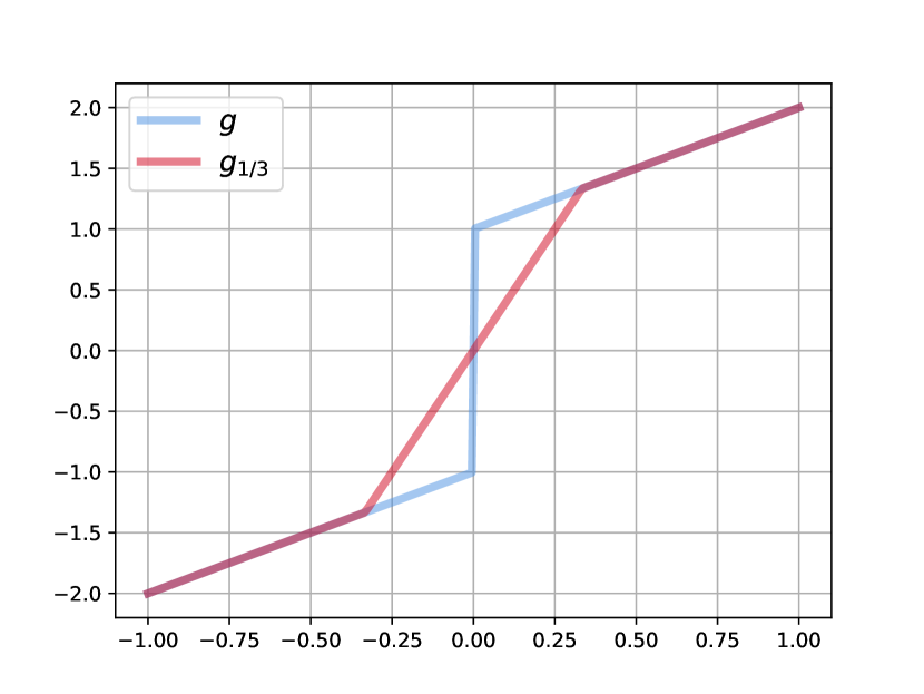
(a) Illustration of the maps $g$ from Eq. 9 and $g_{\varepsilon}$ from Eq. 10 with $\varepsilon=1/3$.

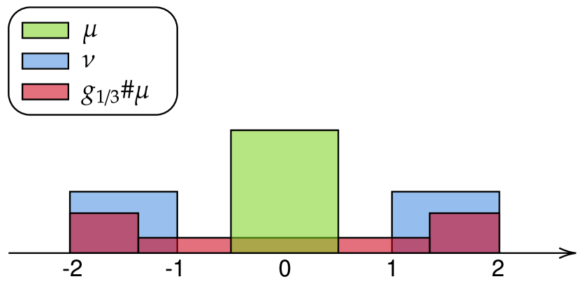
(b) Illustration of the image measure $g_{1/3}\#\mu$ with $\mu=\mathcal{U}([-1,1])$ and $g_{\varepsilon}$ from Eq. 10.

Figure 2: Illustration of the counter-example to existence.

It follows that $g_{\varepsilon}\#\mu$ converges weakly towards $\nu$ as $\varepsilon\longrightarrow 0$. As a result, since the measures are compactly supported, $\mathrm{W}_{2}^{2}(g_{\varepsilon}\#\mu,\nu)\xrightarrow[\varepsilon\longrightarrow 0]{}0$, thus the value of Problem Eq. 8 is 0.

To conclude, if Problem Eq. 8 had a solution $g$, then it would be continuous and verify $\mathrm{W}_{2}^{2}(g\#\mu,\nu)=0$ (since the problem value is 0), thus $g\#\mu=\nu$, which is impossible by the connectivity argument. Therefore, the problem defined in Eq. 8 does not have a solution.

2.6 Discussion on Uniqueness

A natural question is the uniqueness of a solution of the problem

$$\underset{g\in G}{\operatorname{argmin}}\ \mathcal{T}_{c}(g\#\mu,\nu),$$

in the case where the measures, the cost and the class $G$ satisfy the conditions of Theorem 2.5, guaranteeing existence. A first negative answer concerns the simple case where $\mu,\nu$ are discrete and at least two-dimensional. For instance, consider

$$\mu:=\frac{1}{2}(\delta_{(-1,0)}+\delta_{(1,0)}),\quad\nu:=\frac{1}{2}(\delta_{(0,-1)}+\delta_{(0,1)}).$$

Then there are two distinct maps $g_{1},g_{2}$ both verifying $g_{i}\#\mu=\nu$, which are characterised in $L^{2}(\mu)$ by their values on the two points $(\pm 1,0)$.

$$g_{1}((-1,0))=(0,-1),\;g_{1}((1,0))=(0,1),\quad g_{2}((-1,0))=(0,1),\;g_{2}((1,0))=(0,-1),$$

as we illustrate in Fig. 3.

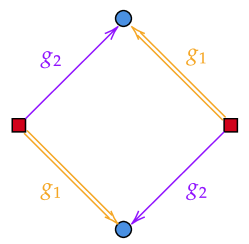
Figure 3: A simple case with two transport maps between 2-point discrete measures in $\mathbb{R}^{2}$.

The previous example illustrates a potential issue for uniqueness, which is the multiplicity of the set $\{g\in G\ |\ g\#\mu=\nu\}$. Another simple counter-example to uniqueness which stems from this property is for $\mu=\nu=\mathcal{N}(0,I)$ the standard $d$-variate Gaussian distribution. In this case, any rotation $R$ verifies $R\#\mathcal{N}(0,I)=\mathcal{N}(0,I)$.

More generally, Brenier’s polar factorisation theorem [7] sheds a light on our invariance issue. We present the theorem below for completeness, see also [32] Section 1.7.2.

Theorem 2.15 (Brenier’s Polar Factorisation [7]).

Let $\mathcal{K}\subset\mathbb{R}^{d}$ a compact set, and $g:\mathcal{K}\longrightarrow\mathbb{R}^{d}$. Consider $\mathscr{L}_{\mathcal{K}}$ the rescaled Lebesgue measure on $\mathcal{K}$, suppose that $g\#\mathscr{L}_{\mathcal{K}}\ll\mathscr{L}$, then there exists a unique ($\mathscr{L}$-almost-everywhere) decomposition $g=(\nabla\varphi)\circ s$ such that:

• $\varphi:\mathcal{K}\longrightarrow\mathbb{R}^{d}$ is convex;

• $s:\mathcal{K}\longrightarrow\mathcal{K}$ is measure-preserving, which is to say that $s\#\mathscr{L}_{\mathcal{K}}=\mathscr{L}_{\mathcal{K}}$.

To fix the ideas, if we consider $\mu=\mathscr{L}_{[0,1]^{d}}$, we can fix $g\in G$ and assume sufficient regularity, then decompose $g=\nabla\varphi\circ s$. Then any map $h$ of the form $\nabla\varphi\circ r$ with $r$ a measure-preserving map will verify $h\#\mathscr{L}_{[0,1]^{d}}=g\#\mathscr{L}_{[0,1]^{d}}$. To avoid such potential counter-examples, we will focus on the case where $G$ is a subset of gradients of convex functions.

We provide a uniqueness result for the $\mathrm{W}_{2}$ case, under the simplifying assumption that $\nu=\mu$. Note that if $L<1$, the identity map does not belong in $G$, and there does not exist a $g\in G$ such that $g\#\mu=\mu$.

Proposition 2.16.

Suppose that

$$G=\left\{g:\mathbb{R}^{d}\longrightarrow\mathbb{R}^{d}:g=\nabla\varphi\ \mathscr{L}-\text{a.e.},\;\varphi\ \text{convex},\;g\ L-\text{Lipschitz}\right\},$$

and that $\mu\in\mathcal{P}_{2}(\mathbb{R}^{d})$ with $\mu\ll\mathscr{L}$. Then if $g_{0}$ and $g_{1}$ are solutions of the problem

$$\underset{g\in G}{\operatorname{argmin}}\ \mathrm{W}_{2}^{2}(g\#\mu,\mu),$$

then $g_{0}=g_{1}$ everywhere on $\operatorname{supp}(\mu)$.

Proof.

We will show that if $g_{0}$ and $g_{1}$ are solutions, then $g_{0}\#\mu=g_{1}\#\mu$. First, one may write $g_{i}=\nabla\varphi_{i}$ with $\varphi_{i}$ convex (for $i=0,1$). By [32] Theorem 1.48 (we remind that by Lemma 2.2, $g_{i}\#\mu\in\mathcal{P}_{2}(\mathbb{R}^{d})$), since $\varphi_{i}$ is convex, $g_{i}$ is the optimal transport map between $\mu$ and $\nabla\varphi_{i}\#\mu$. Consider for $t\in[0,1]$ the interpolation $g_{t}:=(1-t)g_{0}+tg_{1}$. Then by definition (see [3], Section 9.2), the curve $(g_{t}\#\mu)_{t\in[0,1]}$ is a generalised geodesic between $g_{0}\#\mu$ and $g_{1}\#\mu$ with respect to the base measure $\mu$. This allows us to apply [3] Lemma 9.2.1, specifically Equation 9.2.7c, which yields

$$\forall t\in[0,1],\;\mathrm{W}_{2}^{2}(g_{t}\#\mu,\mu)\leq(1-t)\mathrm{W}_{2}^{2}(g_{0}\#\mu,\mu)+t\mathrm{W}_{2}^{2}(g_{1}\#\mu,\mu)-t(1-t)\mathrm{W}_{2}^{2}(g_{0}\#\mu,g_{1}\#\mu).$$

The curvature of this generalised geodesic will allow us to build a better solution if $g_{0}\#\mu\neq g_{1}\#\mu$, as we illustrate in Fig. 4.

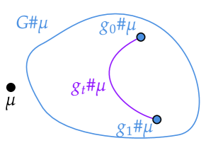
Figure 4: The generalised geodesic based on $\mu$ between $g_{0}\#\mu$ and $g_{1}\#\mu$.

Taking $t=1/2$ yields, using the optimality of $g_{0}$ and $g_{1}$ and writing $v$ for the problem value:

$$\mathrm{W}_{2}^{2}(g_{\frac{1}{2}}\#\mu,\mu)\leq v-\frac{1}{4}\mathrm{W}_{2}^{2}(g_{0}\#\mu,g_{1}\#\mu).$$

Since $G$ is convex, we have $g_{\frac{1}{2}}\in G$, which imposes $\mathrm{W}_{2}^{2}(g_{0}\#\mu,g_{1}\#\mu)=0$, since $v$ is the optimal problem value. We conclude $g_{0}\#\mu=g_{1}\#\mu$. However, as stated earlier, by [32] Theorem 1.48, $g_{i}$ is the optimal transport map between $\mu$ and $g_{i}\#\mu$ for $i=0,1$. By uniqueness of the optimal transport map in this setting, we conclude $g_{0}=g_{1}$. (The equality holds $\mu$-a.e., then since $g_{0}$ and $g_{1}$ are assumed Lipschitz, this shows equality everywhere on $\operatorname{supp}(\mu)$.) ∎

Remark 2.17.

One could replace the set $G$ in 2.16 by a convex subset of $G$, the proof of the result would follow verbatim.

Remark 2.18.

The problem in 2.16 is related to the problem of the Wasserstein metric projection, which was studied in [11] (see Section 5), from which the curvature argument in our proof was closely inspired. This Wasserstein projection problem was also studied for $\mathrm{W}_{p}^{p}$ in [1].

Remark 2.19.

Under some assumptions, it may be possible to find subclasses of gradients of convex functions $G$ such that the set $G\#\mu\subset\mathcal{P}_{2}(\mathbb{R}^{d})$ is geodesically convex (with respect to $\mathrm{W}_{2}$ geodesics): take $g_{0},g_{1}\in G$, assume that $g_{0}\#\mu\ll\mathscr{L}$ (Lemma A.5 provides a sufficient condition on $g_{0}$ and $\mu$ for this to be the case). Then the $\mathrm{W}_{2}$ geodesic from $g_{0}\#\mu$ to $g_{1}\#\mu$ is

$$\nu_{t}:=((1-t)I+tT)\#g\#\mu_{0},$$

where $T$ is the optimal transport map from $g_{0}\#\mu$ to $g_{1}\#\mu$, which is uniquely defined thanks to Brenier’s Theorem (see [32], Theorem 1.22 for a possible reference without compactness assumptions). Since $(T\circ g_{0})\#\mu=g_{1}\#\mu$, under some regularity assumptions, it may be possible to show that $T\circ g_{0}=g_{1}$ using the Monge-Ampère equation, then $((1-t)I+tT)\circ g_{0}=(1-t)g_{0}+tg_{1}\in G$. In this case, the generalised geodesic based on $\mu$ coincides with the $\mathrm{W}_{2}$ geodesic between $g_{0}\#\mu$ and $g_{1}\#\mu$.

Unfortunately, $\rho\longmapsto\mathrm{W}_{2}^{2}(\rho,\nu)$ is not convex along $\mathrm{W}_{2}$ geodesics, since it satisfies the opposite inequality ([3], Theorem 7.3.2). As a result, even if we found a convex class $G$ of gradients of convex functions such that $G\#\mu$ were geodesically convex, curvature arguments would not yield uniqueness immediately. Intuition suggests that in some sense, the problem minimises a concave function over a convex set, which bodes poorly with uniqueness.

In Section 3.2, we shall study the case $d=1$ and show uniqueness and an explicit expression for the minimiser of the map problem for non-decreasing functions $g$ and the squared Euclidean cost.

2.7 The Plan Approximation Problem

In some cases, one may have access to a transport plan between two measures $\mu,\nu$, which poses the natural question of finding a map that approximates this transport plan. For instance, one may compute the optimal entropic plan [9], a Gaussian-Mixture-Model optimal plan [12], or an optimal transport plan for a cost that does not verify the twist condition (see [32] Definition 1.16).

Given a cost $C:(\mathbb{R}^{k}\times\mathbb{R}^{d})\times(\mathbb{R}^{k}\times\mathbb{R}^{d})\longrightarrow\mathbb{R}_{+}$, and measures $\mu\in\mathcal{P}(\mathbb{R}^{k}),\nu\in\mathcal{P}(\mathbb{R}^{d})$, we will want to approximate a plan $\gamma\in\Pi(\mu,\nu)$ by the image measure $(I,g)\#\mu$, where $I$ denotes the identity map of $\mathbb{R}^{k}$. We define the Constrained Approximate Transport Plan problem as:

$$\underset{g\in G}{\operatorname{argmin}}\ \mathcal{T}_{C}((I,g)\#\mu,\gamma).$$ (12)

Similarly to Eq. 3, the transport cost in Eq. 12 can be re-written using the change-of-variables formula (Lemma 2.1):

$$\mathcal{T}_{C}((I,g)\#\mu,\gamma)=\underset{\rho\in\Pi(\mu,\gamma)}{\min}\ \int_{\mathbb{R}^{k}\times(\mathbb{R}^{k}\times\mathbb{R}^{d})}C\left((x,g(x)),(y_{1},y_{2})\right)\mathrm{d}\rho(x,y_{1},y_{2}).$$ (13)

To begin with, one may cast Eq. 12 as a map problem (Eq. 3), providing existence automatically under adequate conditions.

Corollary 2.20.

Consider the class of functions

$$H:=\{h:\mathbb{R}^{k}\longrightarrow\mathbb{R}^{k}\times\mathbb{R}^{d}\ :\ h=(x,y)\longmapsto(x,g(y)),\;g\in G\},$$

the map problem (Eq. 3) is a particular map problem (Eq. 12):

$$\underset{g\in G}{\min}\ \mathcal{T}_{C}((I,g)\#\mu,\gamma)=\underset{h\in H}{\min}\ \mathcal{T}_{C}(h\#\mu,\gamma),$$

hence existence holds by Theorem 2.5 if the conditions of the theorem are verified by $C,G$ and the measures $\mu,\gamma$.

Remark 2.21.

In the light of Remark 2.8, one could replace the input space $\mathbb{R}^{k}$ and the target space $\mathbb{R}^{d}$ by Polish spaces $\mathcal{X}$ and $\mathcal{Y}$ verifying the Heine-Borel property, in which case condition 1) would ask for $(x_{1},x_{2})\longmapsto C((x_{1},x_{2}),(y_{1},y_{2}))$ to be proper.

We shall see that in certain cases, the two problems Eq. 12 and Eq. 3 are in fact equivalent.

Proposition 2.22.

Consider a cost $C$ of the separable form $C((x_{1},x_{2}),(y_{1},y_{2}))=h(c_{1}(x_{1},y_{1}),c_{2}(x_{2},y_{2}))$, where $h:\mathbb{R}_{+}\times\mathbb{R}_{+}\longrightarrow\mathbb{R}_{+}$, $c_{1}:\mathbb{R}^{k}\times\mathbb{R}^{k}\longrightarrow\mathbb{R}_{+}$ and $c_{2}:\mathbb{R}^{d}\times\mathbb{R}^{d}$ are continuous, with $\forall x\in\mathbb{R}^{k},\;c_{1}(x,x)=0$, and $\forall u,v\in\mathbb{R}_{+},\;h(u,v)\geq v$ and $h(0,v)=v$. Let $g:\mathbb{R}^{k}\longrightarrow\mathbb{R}^{d}$ a measurable function, $\nu\in\mathcal{P}(\mathbb{R}^{d})$ and $\mu\in\mathcal{P}(\mathbb{R}^{k})$. Let $\gamma\in\Pi(\mu,\nu)$ a plan between $\mu$ and $\nu$.

We assume that the values $\mathcal{T}_{C}((I,g)\#\mu,\gamma)$ is finite. We have the equality

$$\mathcal{T}_{c_{2}}(g\#\mu,\nu)=\mathcal{T}_{C}((I,g)\#\mu,\gamma).$$

Proof.

For $\rho\in\Pi(\mu,\gamma)$, let $A(\rho):=\int_{\mathbb{R}^{k}\times(\mathbb{R}^{k}\times\mathbb{R}^{d})}C((x,g(x)),(y_{1},y_{2}))\mathrm{d}\rho(x,y_{1},y_{2})<+\infty$, and denote $A^{*}:=\mathcal{T}_{C}((I,g)\#\mu,\gamma)$. Likewise, for $\pi\in\Pi(\mu,\nu),$ let $B(\pi):=\displaystyle\int_{\mathbb{R}^{k}\times\mathbb{R}^{d}}c_{2}(g(x),y)\mathrm{d}\pi(x,y)$, and $B^{*}:=\mathcal{T}_{c_{2}}(g\#\mu,\nu).$

First, we prove $A^{*}\leq B^{*}$. By [32], Theorem 1.7, there exists $\pi^{*}\in\Pi(\mu,\nu)$ such that $B^{*}=B(\pi^{*})$. Define $\rho\in\Pi(\mu,\gamma)$ a measure such that for each test function $f$,

$$\int_{\mathbb{R}^{k}\times(\mathbb{R}^{k}\times\mathbb{R}^{d})}f(x,y_{1},y_{2})\mathrm{d}\rho(x,y_{1},y_{2})=\displaystyle\int_{\mathbb{R}^{k}\times\mathbb{R}^{d}}f(y_{1},y_{1},y_{2})\mathrm{d}\pi^{*}(y_{1},y_{2}),$$

or symbolically “$\rho(\mathrm{d}x\mathrm{d}y_{1}\mathrm{d}y_{2})=\delta_{y_{1}}(\mathrm{d}x)\pi^{*}(\mathrm{d}y_{1}\mathrm{d}y_{2})$". Then, since $h(c_{1}(y_{1},y_{1}),c_{2}(g(y_{1}),y_{2}))=0$, we have

$$A^{*}\leq A(\rho)=\displaystyle\int_{\mathbb{R}^{k}\times(\mathbb{R}^{k}\times\mathbb{R}^{d})}h(c_{1}(y_{1},y_{1}),c_{2}(g(y_{1}),y_{2}))\mathrm{d}\pi^{*}(y_{1},y_{2})\leq\displaystyle\int_{\mathbb{R}^{k}\times\mathbb{R}^{d}}c_{2}(g(y_{1}),y_{2})\mathrm{d}\pi^{*}(y_{1},y_{2})=B^{*}.$$

Now for $A^{*}\geq B^{*}$, we let $\rho\in\Pi(\mu,\gamma)$. Using $h(u,v)\geq v,$ we have

$$A(\rho)=\displaystyle\int_{\mathbb{R}^{k}\times(\mathbb{R}^{k}\times\mathbb{R}^{d})}h(c_{1}(x,y_{1}),c_{2}(g(x),y_{2}))\mathrm{d}\rho(x,y_{1},y_{2})\geq\displaystyle\int_{\mathbb{R}^{k}\times(\mathbb{R}^{k}\times\mathbb{R}^{d})}c_{2}(g(x),y_{2})\mathrm{d}\rho(x,y_{1},y_{2}).$$

Again, we can define $\pi\in\Pi(\mu,\nu)$ such that for any test function $f$,

$$\int_{\mathbb{R}^{k}\times\mathbb{R}^{d}}f(x,y_{2})\mathrm{d}\pi(x,y_{2})=\displaystyle\int_{\mathbb{R}^{k}\times(\mathbb{R}^{k}\times\mathbb{R}^{d})}f(x,y_{2})\mathrm{d}\rho(x,y_{1},y_{2}),$$

and notice

$$\int_{\mathbb{R}^{k}\times(\mathbb{R}^{k}\times\mathbb{R}^{d})}c_{2}(g(x),y_{2})\mathrm{d}\rho(x,y_{1},y_{2})=B(\pi)\geq B^{*},$$

which yields $A^{*}\geq B^{*}$. ∎

For example, the cost $C(x,y)=\|x-y\|_{2}^{2}$ satisfies these conditions (with $h(u,v)=u+v$), and thus the problems Eq. 3 and Eq. 12 are equivalent. This is still the case for costs of the form $C=\|\cdot-\cdot\|_{p}^{qp}$ for $p\geq 1$ and $q>0$, in which case one takes $h(u,v)=(u^{1/q}+v^{1/q})^{q}$. For $C((x_{1},x_{2}),(y_{1},y_{2}))=\|(x_{1},x_{2})-(y_{1},y_{2})\|_{\infty}^{p}$, this is also the case with $c_{1,2}(x,y)=\|x-y\|_{\infty}^{p}$ and $h(u,v)=\max(u,v)$.

In particular, a possible choice of norm on the product space is $\|x\|_{\Sigma}=(x^{\top}\Sigma^{-1}x)^{1/2}$ for $\Sigma$ symmetric positive-definite. This choice is of interest since the cost $C((x_{1},x_{2}),(y_{1},y_{2}))=\|(x_{1},x_{2})-(y_{1},y_{2})\|_{\Sigma}^{2}$ is quadratic (which is desirable for numerics), but does not satisfy the equivalence condition from 2.22 as soon as $\Sigma$ is not block-diagonal.

In Fig. 5, we illustrate the plan approximation problem for the quadratic cost for two different plans: the Entropic Optimal Transport plan [27] and the Gaussian Mixture Model OT plan [12]. The numerics where done using the tools presented in Section 4.2. Note that the plan approximation is equivalent to a map problem in this case, and has a particular structure due to the one-dimensional setting, hence we emphasise that Fig. 5 is merely an illustration of the problem at hand.

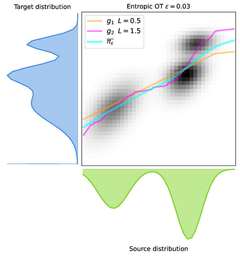
(a) plan approximation solutions for the Entropic-OT plan [27].

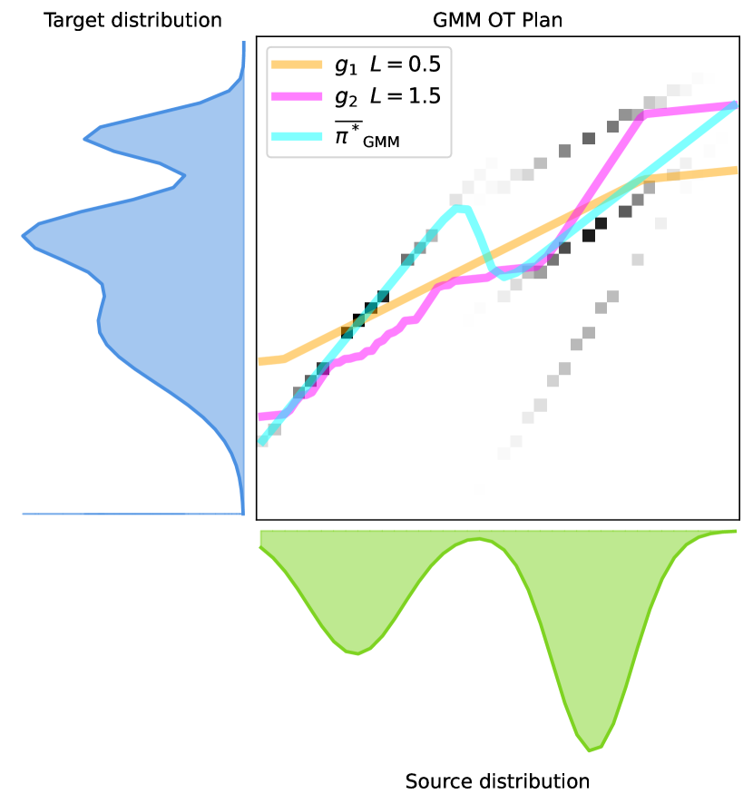
(b) Illustration of plan approximation solutions for the GMM-OT plan [12].

Figure 5: Illustration of solutions of plan approximation problems (Eq. 12), for two different plans between Gaussian Mixtures. We compare the plans with $L=1/2$ and $L=3/2$-Lipschitz solutions, as well as to the barycentric projection of the given plans (see Section 3.1).

3 Alternate Minimisation in the Squared Euclidean Case

For any continuous cost $c:\mathbb{R}^{d}\times\mathbb{R}^{d}\longrightarrow\mathbb{R}_{+}$, the map problem Eq. 3 is a minimisation problem over $\pi\in\Pi(\mu,\nu)$ and $g\in G$:

$$\underset{g\in G}{\min}\ \underset{\pi\in\Pi(\mu,\nu)}{\min}\ \int_{\mathcal{X}\times\mathbb{R}^{d}}c(g(x),y)\mathrm{d}\pi(x,y).$$

In this section, we study this alternate minimisation problem in the case where $c(x,y)=\|x-y\|_{2}^{2}$.

When $\pi\in\Pi(\mu,\nu)$ is fixed, the sub-problem has the particular structure

$$\underset{g\in G}{\min}\ \int_{\mathcal{X}\times\mathbb{R}^{d}}\|g(x)-y\|_{2}^{2}\mathrm{d}\pi(x,y).$$ (14)

To ensure the finiteness of the cost, we assume that $\nu\in\mathcal{P}_{2}(\mathbb{R}^{d})$ and that $\forall g\in G,\;g\#\mu\in\mathcal{P}_{2}(\mathbb{R}^{d})$. We shall see in Section 3.1 that the problem in (Eq. 14) is equivalent to the $L^{2}$ projection of the barycentric map $\overline{\pi}$ onto the set $G$, provided that $G$ is a convex and closed subset of $L^{2}(\mu)$.

When $g\in G$ is fixed, the problem reads

$$\underset{\pi\in\Pi(\mu,\nu)}{\min}\ \int_{\mathcal{X}\times\mathbb{R}^{d}}\|g(x)-y\|_{2}^{2}\mathrm{d}\pi(x,y),$$ (15)

and can be seen from two different viewpoints: either as the squared Euclidean optimal transport problem between $g\#\mu$ and $\nu$ (i.e. $\mathrm{W}_{2}^{2}(g\#\mu,\nu)$), or as the optimal transport problem with cost $c(x,y):=\|g(x)-y\|_{2}^{2}$ between $\mu$ and $\nu$. If $g\#\mu$ is absolutely continuous and $\nu$ is discrete, then Eq. 15 is a semi-discrete OT problem. We provide sufficient conditions on $g$ for this to be the case in Section A.2.

This alternate minimisation viewpoint poses a natural question: if $\pi:=\pi^{*}\in\Pi^{*}(\mu,\nu)$ is an optimal plan between $\mu$ and $\nu$, does the following equality holds?

$$\underset{g\in G}{\operatorname{argmin}}\ \underset{\pi\in\Pi(\mu,\nu)}{\min}\ \int_{\mathcal{X}\times\mathbb{R}^{d}}\|g(x)-y\|_{2}^{2}\mathrm{d}\pi(x,y)\;\stackrel{{\scriptstyle\mathclap{\mbox{?}}}}{{=}}\;\underset{g\in G}{\operatorname{argmin}}\ \int_{\mathcal{X}\times\mathbb{R}^{d}}\|g(x)-y\|_{2}^{2}\mathrm{d}\pi^{*}(x,y).$$ (16)

In Section 3.2, we prove that this equality holds in the one-dimensional case $\mathcal{X}=\mathbb{R}^{d}=\mathbb{R}$ and if $G$ is a subclass of non-decreasing functions, thus generalizing a result of [26]. We also provide a counter-example of this property when $d\geq 2$ in Section 3.3.

3.1 Projection of the Barycentric Map

In this section, we will show that the sub-problem with $\pi\in\Pi(\mu,\nu)$ fixed can be written as the following $L^{2}$ projection problem:

$$\underset{g\in G}{\operatorname{argmin}}\ \int_{\mathcal{X}\times\mathbb{R}^{d}}\|g(x)-y\|_{2}^{2}\mathrm{d}\pi(x,y)=\underset{g\in G}{\operatorname{argmin}}\ \|g-\overline{\pi}\|_{L^{2}(\mu)}^{2},$$

where $\overline{\pi}$ is the barycentric projection of $\pi$ (defined below), and $L^{2}(\mu)$ is a shorthand for $L^{2}(\mu;\mathbb{R}^{d})$, the space of measurable functions $T:\mathcal{X}\longrightarrow\mathbb{R}^{d}$ such that $\int_{\mathcal{X}}\|T(x)\|_{2}^{2}\mathrm{d}\mu(x)<+\infty$. We begin by briefly introducing the notion of barycentric projection.

The barycentric projection of $\pi$ is the map $\overline{\pi}:\mathbb{R}^{d}\longrightarrow\mathbb{R}^{d}$ defined for $\mu$-almost all $x\in\mathbb{R}^{d}$ by

$$\overline{\pi}(x)=\mathbb{E}_{(X,Y)\sim\pi}[Y|X=x],$$ (17)

If $\pi$ admits a disintegration with respect to its first marginal $\mu$ of the form $\pi(\mathrm{d}x\mathrm{d}y)=\pi_{x}(\mathrm{d}y)\mu(\mathrm{d}x)$, then

$$\overline{\pi}(x)=\displaystyle\int_{\mathbb{R}^{d}}y\,\mathrm{d}\pi_{x}(y).$$

Since the conditional expectation minimises the $L^{2}$ distance, we also have

$$\overline{\pi}=\underset{T\in L^{2}(\mu)}{\operatorname{argmin}}\displaystyle\int_{\mathbb{R}^{2d}}\|y-T(x)\|_{2}^{2}\mathrm{d}\pi(x,y),$$ (18)

where the equality is to be understood in $L^{2}(\mu)$. Another interesting property is that if $\pi=\pi^{*}\in\Pi^{*}(\mu,\nu)$ is an optimal transport plan between $\mu$ and $\nu$ with respect to the squared Euclidean distance cost, then by [3], Section 6.2.3, there exists $\varphi:\mathbb{R}^{d}\longrightarrow\mathbb{R}$ convex such that for $\pi^{*}$-almost-every $(x,y)\in\mathbb{R}^{2d}$, we have $y\in\partial\varphi(x)$, where $\partial\varphi(x)$ denotes the Fréchet sub-differential of $\varphi$:

$$y\in\partial\varphi(x)\Longleftrightarrow\underset{z\longrightarrow x}{\liminf}\ \cfrac{\varphi(z)-\varphi(x)-\langle y,z-x\rangle}{\|x-z\|_{2}}\geq 0.$$

Since the Fréchet sub-differential of a convex function is convex, it follows that for $\mu$-almost every $x\in\mathbb{R}^{d},\;\overline{\pi^{*}}(x)\in\partial\varphi(x)$.

If we require constraints on $T$ in Eq. 18, we obtain exactly the sub-problem of the map problem with a fixed plan $\pi$ (Eq. 14), which we reproduce below:

$$\underset{g\in G}{\operatorname{argmin}}\ \displaystyle\int_{\mathcal{X}\times\mathbb{R}^{d}}\|g(x)-y\|_{2}^{2}\mathrm{d}\pi(x,y).$$

For this reason, we call this problem the Constrained Barycentric Map problem. A consequence of the proof of Theorem 2.5 is that this problem has a solution. If $G$ is a convex set and closed in $L^{2}(\mu)$, then existence and uniqueness are guaranteed by the Hilbert projection Theorem. Since $\overline{\pi}$ minimises the $L^{2}$ distance, it is a solution of Eq. 14 if it is in $G$.

Using the fact that the barycentric projection is an $L^{2}$ projection (Eq. 18), one may re-write the Projected Barycentric Map Problem Eq. 14 as an $L^{2}$ minimisation with respect to the barycentric projection:

Proposition 3.1.

Let $\pi\in\Pi(\mu,\nu)$ and $f:\mathcal{X}\longrightarrow\mathbb{R}^{d}$ a measurable function. Then one has

$$\int_{\mathcal{X}\times\mathbb{R}^{d}}\|f(x)-y\|_{2}^{2}\mathrm{d}\pi(x,y)=\displaystyle\int_{\mathcal{X}}\|f(x)-\overline{\pi}(x)\|_{2}^{2}\mathrm{d}\mu(x)+\displaystyle\int_{\mathcal{X}\times\mathbb{R}^{d}}\|y-\overline{\pi}(x)\|_{2}^{2}\mathrm{d}\pi(x,y),$$ (19)

and as a result, the Projected Barycentric Map problem Eq. 14 is equivalent to the problem

$$\underset{g\in G}{\operatorname{argmin}}\ \displaystyle\int_{\mathcal{X}}\|g(x)-\overline{\pi}(x)\|_{2}^{2}\mathrm{d}\mu(x).$$ (20)

Moreover, the second term on the right-hand side of Eq. 19 only depends on $\overline{\pi}$ and the measures $\mu,\nu$ (it doesn’t depend on $\pi$). More precisely, we have

$$\int_{\mathcal{X}\times\mathbb{R}^{d}}\|y-\overline{\pi}(x)\|_{2}^{2}\mathrm{d}\pi(x,y)=m_{2}(\nu)-m_{2}(\overline{\pi}\#\mu),$$

where $m_{2}(\rho):=\int\|x\|_{2}^{2}\mathrm{d}\rho(x)$ for a positive measure $\rho$.

Proof.

Denote $J$ the left-hand-side of Eq. 19, and compute (taking the expectation under $(X,Y)\sim\pi$)

$$J =\mathbb{E}\left[\|Y-f(X)\|_{2}^{2}\right]=\mathbb{E}\left[\|Y-\overline{\pi}(X)+\overline{\pi}(X)+f(X)\|_{2}^{2}\right]$$

$$=\mathbb{E}\left[\|Y-\overline{\pi}(X)\|_{2}^{2}\right]+\mathbb{E}\left[\|\overline{\pi}(X)+f(X)\|_{2}^{2}\right]+2\mathbb{E}\left[(Y-\overline{\pi}(X))^{T}(\overline{\pi}(X)+f(X))\right],$$

then since $\overline{\pi}(X)$ is the orthogonal projection of $Y$ onto the set of random variables that are functions of $X$, the inner product $\mathbb{E}\left[(Y-\overline{\pi}(X))^{T}(\overline{\pi}(X)+f(X))\right]$ is zero, yielding Eq. 19.

We can expand the norm in the second term of the right-hand side of Eq. 19 using $m_{2}(\nu)$ the second moment of $\nu$ and get

$$\displaystyle\int_{\mathcal{X}\times\mathbb{R}^{d}}\|y-\overline{\pi}(x)\|_{2}^{2}\mathrm{d}\pi(x,y) =m_{2}(\nu)-2\displaystyle\int_{\mathcal{X}\times\mathbb{R}^{d}}y\cdot\overline{\pi}(x)\mathrm{d}\pi(x,y)+\displaystyle\int_{\mathcal{X}}\|\overline{\pi}(x)\|_{2}^{2}\mathrm{d}\mu(x).$$

Writing the disintegration of $\pi$ w.r.t. $\mu$ as $\pi(\mathrm{d}x,\mathrm{d}y)=\pi_{x}(\mathrm{d}y)\mu(\mathrm{d}x)$, we re-write the second term as

$$\int_{\mathcal{X}\times\mathbb{R}^{d}}y\cdot\overline{\pi}(x)\mathrm{d}\pi(x,y)=\int_{\mathcal{X}}\overline{\pi}(x)\cdot\left(\int_{\mathbb{R}^{d}}y\mathrm{d}\pi_{x}(y)\right)\mathrm{d}\mu(x)=\displaystyle\int_{\mathcal{X}}\overline{\pi}(x)\cdot\overline{\pi}(x)\mathrm{d}\mu(x)=m_{2}(\overline{\pi}\#\mu).$$

Putting our computations together yields

$$\int_{\mathcal{X}\times\mathbb{R}^{d}}\|y-\overline{\pi}(x)\|_{2}^{2}\mathrm{d}\pi(x,y)=m_{2}(\nu)-m_{2}(\overline{\pi}\#\mu).$$

∎

Remark 3.2 (Ties to the Convex Least Squares Estimator [22].).

In [22], Manole et al. study the statistical properties of various estimators of Optimal Transport maps, assuming some regularity on the input distributions. Specifically, they introduce the so-called Convex Least Squares Estimator: given $\hat{\mu}_{n}:=\frac{1}{n}\sum_{i=1}^{n}\delta_{x_{i}}$ with the $(x_{i})$ being i.i.d. samples of $\mu$ and $\hat{\nu}_{m}:=\frac{1}{m}\sum_{j=1}^{m}\delta_{y_{j}}$ with the $(y_{j})$ i.i.d. samples of $\nu$, the estimator is defined as

$$\hat{T}_{n,m}=\nabla\hat{\varphi},\quad\hat{\varphi}\in\underset{\varphi\in\Phi_{L}}{\operatorname{argmin}}\ \displaystyle\sum\limits_{i=1}^{n}\displaystyle\sum\limits_{j=1}^{m}\hat{\pi}^{*}_{i,j}\|\nabla\varphi(x_{i})-y_{j}\|_{2}^{2},$$ (21)

where $\hat{\pi}^{*}$ is an optimal transport plan between $\hat{\mu}_{n}$ and $\hat{\nu}_{m}$, and where $\Phi_{L}$ is the set of $\mathcal{C}^{1}$ convex functions from $\Omega\subset\mathbb{R}^{d}$ to $\mathbb{R}$ with a $L$-Lipschitz gradient. Notice that Eq. 21 is a Constrained Barycentric Projection problem Eq. 14 with a specific (discrete) transport plan $\hat{\pi}^{*}$, chosen to be the optimal transport plan between $\hat{\mu}_{n}$ and $\hat{\nu}_{m}$, and with the particular class $G:=\mathcal{F}_{\mathcal{E},L,\ell}$ (introduced in Section 2.3).

3.2 Equivalence to a Constrained Barycentric Projection in Dimension 1

In this section, we shall prove that the Constrained Approximate Transport Map problem (Eq. 3) is equivalent to the Constrained Barycentric Projection Problem (Eq. 14) for the quadratic cost in dimension $1$. This provides a positive answer to the question raised in Eq. 16 in this particular case. The idea behind this equivalence stems from the fact that in dimension one, optimal transport maps are non-decreasing, and the composition of two optimal transport maps remains an optimal transport map.

Proposition 3.3.

For $\mu,\nu\in\mathcal{P}_{2}(\mathbb{R})$, and $G$ a subclass of the non-decreasing functions $g:\mathbb{R}\longrightarrow\mathbb{R}$ such that $g\#\mu\in\mathcal{P}_{2}(\mathbb{R})$, we have the equality

$$\underset{g\in G}{\operatorname{argmin}}\ \mathrm{W}_{2}^{2}(g\#\mu,\nu)=\underset{g\in G}{\operatorname{argmin}}\ \|g-\overline{\pi^{*}}\|_{L^{2}(\mu)}^{2},$$ (22)

where $\pi^{*}$ is an optimal transport plan between $\mu$ and $\nu$ for the squared Euclidean cost.

3.3 generalises [26] Proposition 1, which proves the same equivalence for a specific class of functions $G$, and assuming $\mu$ to be either discrete or absolutely continuous with respect to the Lebesgue measure.

The proof of 3.3 hinges on Lemma 3.4, which is intuitive in the absolutely continuous or discrete case, but a bit more technical in full generality. We write below the cumulative distribution function of a probability measure $\rho$ as $F_{\rho}:=x\longmapsto\rho((-\infty,x])$. Since it is non-decreasing, we can define its right-inverse as (using the notation $\overline{\mathbb{R}}:=\mathbb{R}\cup\{-\infty,+\infty\}$)

$$F_{\rho}^{\leftarrow}:\mathbb{R}\longrightarrow\overline{\mathbb{R}}:\quad\forall p\in\mathbb{R},\;F_{\rho}^{\leftarrow}(p):=\inf\left.\left\{x\in\mathbb{R}\ \right|\ F_{\rho}(x)\geq p\right\}.$$

Lemma 3.4.

Let $\mu\in\mathcal{P}(\mathbb{R})$ and $g:\mathbb{R}\longrightarrow\mathbb{R}$ a non-decreasing function, we have the following almost-everywhere change of variables formula for the quantile functions of $g\#\mu$ and $\mu$:

$$F_{g\#\mu}^{\leftarrow}=g\circ F_{\mu}^{\leftarrow},\quad\mathscr{L}_{[0,1]}\text{-almost-everywhere}.$$

Proof.

The proof is provided in Section A.3. ∎

Proof of 3.3 .

Let $g\in G$. By [32] Proposition 2.17 and by Lemma 3.4 successively, we have

$$\mathrm{W}_{2}^{2}(g\#\mu,\nu) =\int_{0}^{1}|F_{g\#\mu}^{\leftarrow}(p)-F_{\nu}^{\leftarrow}(p)|^{2}\mathrm{d}p=\int_{0}^{1}|g\circ F_{\mu}^{\leftarrow}(p)-F_{\nu}^{\leftarrow}(p)|^{2}\mathrm{d}p=\int_{\mathbb{R}^{2}}|g(x)-y|^{2}\mathrm{d}\pi(x,y),$$

where $\pi:=(F_{\mu}^{\leftarrow},F_{\nu}^{\leftarrow})\#\mathscr{L}_{[0,1]}$, which by [32] Theorem 2.9 is the unique optimal plan between $\mu$ and $\nu$ for the squared Euclidean cost. We apply 3.1, which yields

$$\mathrm{W}_{2}^{2}(g\#\mu,\nu)=\int_{\mathbb{R}^{2}}|g(x)-y|^{2}\mathrm{d}\pi(x,y)=\int_{\mathbb{R}}|g(x)-\overline{\pi}(x)|^{2}\mathrm{d}\mu(x)+m_{2}(\nu)-m_{2}(\overline{\pi}\#\mu).$$

Given the expression of the right-hand-side above, we conclude that

$$\underset{g\in G}{\operatorname{argmin}}\ \mathrm{W}_{2}^{2}(g\#\mu,\nu)=\underset{g\in G}{\operatorname{argmin}}\ \|g-\overline{\pi^{*}}\|_{L^{2}(\mu)}^{2},$$

(for any optimal transport plan $\pi^{*}$ between $\mu$ and $\nu$ for the squared Euclidean cost, and we have even remarked that such a plan is in fact unique) since the costs are equal up to a constant independent of $g$. ∎

3.3 Counter-Example to Equivalence to Constrained Barycentric Projection in Dimension 2

In this section, we provide a negative example to the question formulated in Eq. 16, namely that

$$\underset{g\in G}{\operatorname{argmin}}\ \mathrm{W}_{2}^{2}(g\#\mu,\nu)\neq\underset{g\in G}{\operatorname{argmin}}\ \|g-\overline{\pi^{*}}\|_{L^{2}(\mu)},$$

where $\pi^{*}$ is an optimal transport plan (for the squared Euclidean cost) between $\mu$ and $\nu$, in dimension $d\geq 2$. We take $G$ to be the class of monotone continuous functions $g:\mathbb{R}^{2}\longrightarrow\mathbb{R}^{2}$, which is to say that

$$\forall x,y\in\mathbb{R}^{2},\;\langle g(x)-g(y),x-y\rangle\geq 0.$$

Note that gradients of convex functions are monotone, but the converse does not hold. For $(a,b,x)\in(0,+\infty)^{3}$, we consider the following measures:

$$\mu:=\frac{2}{3}\delta_{(0,0)}+\frac{1}{3}\delta_{(x,0)}\text{ and }\nu:=\frac{2}{3}\delta_{(0,0)}+\frac{1}{3}\delta_{(-a,b)}.$$

There is a unique optimal transport plan $\pi^{*}$ between $\mu$ and $\nu$, given by

$$\pi^{*}=\frac{1}{3}\delta_{(0,0)\otimes(0,0)}+\frac{1}{3}\delta_{(0,0)\otimes(-a,b)}+\frac{1}{3}\delta_{(x,0)\otimes(0,0)}.$$

Its barycentric projection is characterised by the following equation

$$\overline{\pi^{*}}(0,0)=(-a/2,b/2)\text{ and }\overline{\pi^{*}}(x,0)=(0,0).$$

We now consider the problem $\underset{g\in G}{\min}\|g-\overline{\pi^{*}}\|_{L^{2}(\mu)}$. A solution of this problem is characterised by its values on the support of $\mu$, and one may reduce the problem to an optimisation over $g(0,0)$ and $g(x,0)$, with the monotonicity constraint $\langle g(0,0)-g(x,0),(0,0)-(x,0)\rangle\geq 0$. Since $\overline{\pi^{*}}$ itself verifies this condition, it is the only solution (in the sense of $L^{2}(\mu)$). We conclude

$$\underset{g\in G}{\operatorname{argmin}}\ \|g-\overline{\pi^{*}}\|_{L^{2}(\mu)}^{2}=\left\{\overline{\pi^{*}}\right\}.$$

We now show that the problem $\underset{g\in G}{\operatorname{argmin}}\ \mathrm{W}_{2}^{2}(g\#\mu,\nu)$ has a different solution set. First, we compute

$$\mathrm{W}_{2}^{2}(\overline{\pi^{*}}\#\mu,\nu)=\frac{a^{2}+b^{2}}{6}.$$

However, if we introduce $g\in G$ such that $g(0,0)=(0,0)$ and $g(x,0)=(0,b)$, we have

$$\mathrm{W}_{2}(g\#\mu,\nu)=\frac{a^{2}}{3}.$$

For instance, $(a,b,x):=(1,10,1)$ yields

$$\mathrm{W}_{2}^{2}(\overline{\pi^{*}}\#\mu,\nu)=\frac{a^{2}+b^{2}}{6}=\frac{101}{6}>\mathrm{W}_{2}^{2}(g\#\mu,\nu)=\frac{a^{2}}{3}=\frac{1}{3}.$$

We illustrate the point configurations for $(a,b,x):=(1,3,1)$ in Fig. 6.

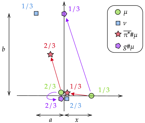
Figure 6: Illustration of the two-dimensional counter-example to the equivalence of the map problem to the $L^{2}$ projection of the barycentric projection. The four points close to $(0,0)$ are represented with an offset for legibility, and represent four points equal to $(0,0)$ exactly.

4 Discrete Measures and Numerical Methods

In this section, we consider some numerical methods to solve the approximate map problem for some specific function classes. In Section 4.1, we consider a simple kernel method which solves a regularised version of Eq. 3. This type of method hinges on the fact that kernel methods yield a finite-dimensional parametrisation of the variable $g$, hence our gradient descent algorithm extends naturally to any parametrised class of functions. In Section 4.2, we present methods in the case where $G$ is the class of $L$-Lipschitz gradients of $\ell$-strongly convex potentials (presented in Section 2.3). For the squared Euclidean cost, these methods were introduced in [26], using convex interpolation results from [35]. We present these methods in additional detail, and introduce a natural generalisation to other costs and regularisations.

4.1 Numerical Method for Maps in a RKHS

We introduce a relatively straightforward kernel method to solve the map problem (Eq. 3). We fix a reproducing kernel Hilbert space (RKHS) $\mathcal{H}$ of functions $\mathcal{X}\longrightarrow\mathbb{R}^{d}$ of kernel $K:\mathcal{X}\times\mathcal{X}\longrightarrow\mathbb{R}^{d\times d}$. We denote by $\langle\cdot,\cdot\rangle_{\mathcal{H}}$ the inner product on $\mathcal{H}$, and $\|\cdot\|_{\mathcal{H}}$ the associated RKHS norm on $\mathcal{H}$.

Given discrete measures $\mu=\sum_{i=1}^{n}a_{i}\delta_{x_{i}}\in\mathcal{P}(\mathcal{X})$ and $\nu=\sum_{j=1}^{m}b_{j}\delta_{y_{j}}\in\mathcal{P}(\mathbb{R}^{d})$, we will solve a regularised variant of the map problem (Eq. 3):

$$\underset{h\in\mathcal{H}}{\operatorname{argmin}}\ \mathcal{T}_{c}(h\#\mu,\nu)+\lambda\|h\|_{\mathcal{H}}^{2},$$ (23)

for some constant $\lambda>0$ that penalises the norm of $h$, which equates to imposing regularity on the function $h$. Given the support of $\mu$, the cost $\mathcal{T}_{c}(h\#\mu,\nu)$ only depends on $(h(x_{1}),\cdots,h(x_{n}))$. A well known reduction method in RKHS theory then allows to look for solutions in the following $n$-dimensional linear subspace $W$ of $\mathcal{H}$:

$$W:=\left\{\sum_{k=1}^{n}K(\cdot,x_{k})u_{k}\ :\ \forall k\in\llbracket 1,n\rrbracket,\;u_{k}\in\mathbb{R}^{d}\right\}.$$ (24)

This fact is known since [5] (Section 3), but given the simplicity of the arguments and for the sake of self-completeness, we provide a proof and presentation in Lemma 4.1.

Lemma 4.1.

Consider a cost function $J:\mathcal{H}\longrightarrow\mathbb{R}_{+}$ which can be written as $J(h)=J\left(h(x_{1}),\cdots,h(x_{n})\right)$. Then if $h^{*}$ is a solution of

$$\underset{h\in\mathcal{H}}{\operatorname{argmin}}\ J(h)+\lambda\|h\|_{\mathcal{H}}^{2},$$

then $h_{W}$, the orthogonal projection of $h^{*}$ onto $W$ (defined in Eq. 24) verifies

$$\forall i\in\llbracket 1,n\rrbracket,\;h_{W}(x_{i})=h^{*}(x_{i}),$$

and as a result $J(h_{W})=J(h^{*})$, which leads to the following problem reduction:

$$\underset{h\in\mathcal{H}}{\operatorname{argmin}}\ J(h)+\lambda\|h\|_{\mathcal{H}}^{2}=\underset{h\in W}{\operatorname{argmin}}\ J(h)+\lambda\|h\|_{\mathcal{H}}^{2}.$$ (25)

Proof.

To show that $\forall i\in\llbracket 1,n\rrbracket,\;h_{W}(x_{i})=h^{*}(x_{i})$, we will show that

$$W^{\perp}=H_{0}:=\left.\left\{h\in\mathcal{H}\ \right|\ \forall i\in\llbracket 1,n\rrbracket,\;h(x_{i})=0\right\}.$$

Indeed,

$$h\in H_{0} \Longleftrightarrow\forall i\in\llbracket 1,n\rrbracket,\;g(x_{i})=0$$

$$\Longleftrightarrow\forall i\in\llbracket 1,n\rrbracket,\;\forall u\in\mathbb{R}^{d},\;g(x_{i})\cdot u=0$$

$$\Longleftrightarrow\forall i\in\llbracket 1,n\rrbracket,\;\forall u\in\mathbb{R}^{d},\;\delta_{x_{i}}^{u}g=0$$

$$\Longleftrightarrow\forall i\in\llbracket 1,n\rrbracket,\;\forall u\in\mathbb{R}^{d},\;\langle g,K(\cdot,x_{i})u\rangle_{\mathcal{H}}=0$$

$$\Longleftrightarrow f\in W^{\perp},$$

where $\delta_{x}^{u}$ is the linear form $h\longmapsto h(x)\cdot u$, whose Riesz representation in $\mathcal{H}$ is $K(\cdot,x)u$ by the kernel reproducing property. We conclude the proof with the fact that as an orthogonal projection, $\|h_{W}\|_{\mathcal{H}}^{2}\leq\|h^{*}\|_{\mathcal{H}}^{2}$, which shows that the cost of $h_{W}$ is less than the cost of $h^{*}$. ∎

Lemma 4.1 allows us to re-write Eq. 23 as a finite-dimensional problem over $W$:

$$\underset{h\in W}{\operatorname{argmin}}\ \mathcal{T}_{c}(h\#\mu,\nu)+\lambda\|h\|_{\mathcal{H}}^{2}.$$ (26)

Since any element $h\in W$ is characterised by its coefficients $(u_{1},\cdots,u_{n})\in(\mathbb{R}^{d})^{n}$, we can formulate Eq. 26 as a problem over the $(u_{i})$. First, using the kernel reproducing property, we compute

$$\left\|\sum_{k=1}^{n}K(\cdot,x_{k})u_{k}\right\|_{\mathcal{H}}^{2}=\sum_{k=1}^{n}\sum_{l=1}^{n}u_{k}^{T}K(x_{k},x_{l})u_{l}.$$ (27)

Concerning the transport cost term, we introduce a notation for the value of the Kantorovich discrete problem

$$\mathrm{W}(a,b,C):=\underset{\pi\in\Pi(\mu,\nu)}{\min}\ C\cdot\pi,$$

and in this case, the cost matrix $C$ can be computed using the expression

$$\forall(i,j)\in\llbracket 1,n\rrbracket\times\llbracket 1,m\rrbracket,\;C_{i,j}=c\left(\sum_{k=1}^{n}K(x_{i},x_{k})u_{k},y_{j}\right).$$ (28)

The dependency in the $(u_{i})$ lies in the cost $C$. Numerically, provided that $c$ is sufficiently regular, this allows a minimisation through classical algorithms such as gradient descent, using differentiable implementations of the discrete Kantorovich cost, such as ot.emd2 [19].

By introducing the $nd\times nd$ matrix $\mathbf{K}$ defined by $n\times n$ blocks $K(x_{i},x_{j})$ of size $d\times d$:

$$\mathbf{K}=\left(\begin{array}[]{ccc}K(x_{1},x_{1})&\cdots&K(x_{1},x_{n})\\ \vdots&&\vdots\\ K(x_{n},x_{1})&\cdots&K(x_{n},x_{n})\end{array}\right),$$

and the stacked vector $\mathbf{u}\in\mathbb{R}^{nd}$, Eqs. 27 and 28 can be re-written as matrix products. This yields our final expression for Eq. 23:

$$\underset{\mathbf{u}\in\mathbb{R}^{nd}}{\min}\ \mathrm{W}(a,b,C(\mathbf{u}))+\lambda\mathbf{u}^{T}\mathbf{K}\mathbf{u},\quad C(\mathbf{u})_{i,j}:=c\left(\mathbf{K}_{[i,:]}\mathbf{u},y_{j}\right),$$ (29)

where $\mathbf{K}_{[i,:]}$ denotes the sub-matrix of $\mathbf{K}$ with the $n$ lines $((i-1)d+1,\cdots,id)$, which corresponds to the $i$-th $d\times d$ block line of $\mathbf{K}$.

Given optimal coefficients $\mathbf{u}=(u_{1},\cdots,u_{n})\in(\mathbb{R}^{d})^{n}$, a solution $h$ is defined everywhere in $\mathcal{X}$ using the kernel:

$$\forall x\in\mathcal{X},\;h(x)=\sum_{i=1}^{n}K(x,x_{i})u_{i}.$$

Remark 4.2.

The only constraints that are imposed upon a solution of Eq. 23 come from the choice of the kernel $K$ (or equivalently of the space $\mathcal{H}$) and of the regularisation coefficient $\lambda>0$. A natural idea would be to add a regularisation term $R(h)$, for instance to enforce $h$ to be a gradient of a convex function. For Lemma 4.1 to apply, one would need to have a regularisation which only depends on the values $(h(x_{i}))$, which is very restrictive. A possible heuristic would be to look for $h\in W$ regardless of this property on $R$, however the resulting problem would have no theoretical link to the problem over $h\in\mathcal{H}$, unlike in our case. Finally, a regularisation which depends on an infinite amount of values $h(x)$ are numerically challenging, in the specific case of dense inequality constraints, we refer to [29] as a useful tool.

Remark 4.3.

A natural idea is to consider class of functions that are perturbations of a simple map, for instance $g=sI+h$, where $h$ is in a RKHS $\mathcal{H}$, and $s>0$ is a scale factor. Given Lemma 4.1, this tweak comes without numerical or theoretical cost.

We illustrate this kernel method in Fig. 7, where we use the Gaussian kernel

$$k(x,y)=\exp\left(-\cfrac{\|x-y\|_{2}^{2}}{2\sigma^{2}}\right).$$

The maps are taken of the form $g=I+h$, where $h$ is in the RKHS generated by the Gaussian kernel.

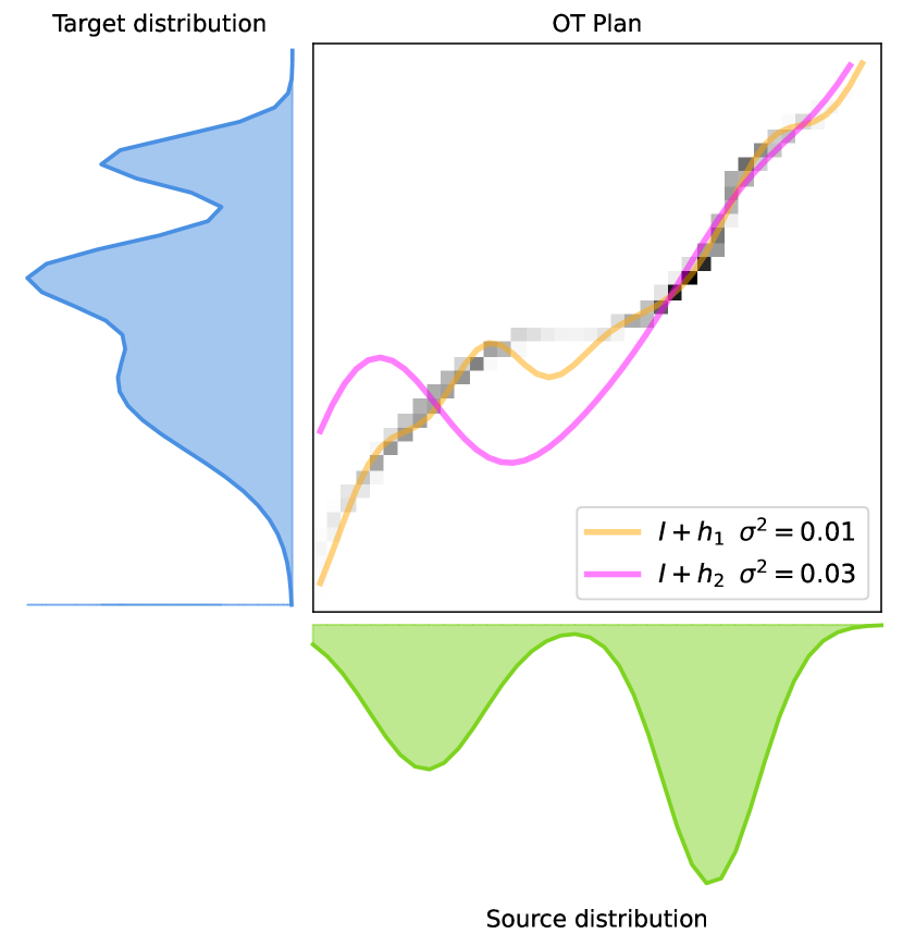
(a) Kernel map solution for a regularisation $\lambda=0.01$ and multiple scales $\sigma^{2}$.

(b) Kernel map solution for a scale $\sigma^{2}=0.01$ and multiple regularisations $\lambda$.

Figure 7: Illustration of the kernel method for the map problem between two Gaussian mixtures, using the Gaussian kernel.

4.2 Numerical Method for Gradients of Convex Functions

In this section, we present numerical methods to solve the approximate problem in the case of the function class $\mathcal{F}_{\mathcal{E},L,\ell}$ of functions $g:\mathbb{R}^{d}\longrightarrow\mathbb{R}^{d}$ that is $L$-Lipschitz and gradient of an $\ell$-strongly convex function $\varphi\in\mathcal{C}^{1}(\mathbb{R}^{d},\mathbb{R})$, on each part $E_{k}$ of the fixed partition $\mathcal{E}$. We already introduced this class in Section 2.3, and it was first considered in the context of map problems by [26]. The numerical methods will aim to solve the problem

$$\underset{\varphi\in\mathcal{F}_{\mathcal{E},L,\ell}}{\operatorname{argmin}}\ \mathcal{T}_{c}(g\#\mu,\nu),$$ (30)

with a particular emphasis on the case where $c$ is quadratic, i.e. $c(x,y)=(x-y)^{T}Q(x-y)+b^{T}(x-y)$, where $Q\in S_{d}^{+}(\mathbb{R})$ is a positive-semi-definite matrix, and $b\in\mathbb{R}^{d}$. For our numerical questions, we consider the discrete case

$$\mu=\sum_{i=1}^{n}a_{i}\delta_{x_{i}},\quad\nu=\sum_{j=1}^{m}b_{j}\delta_{y_{j}}.$$

Obviously, we need to assume that the measure $\mu$ is compatible with the partition, which is to say the the $x_{i}$ are never at the boundary of a part $E_{k}$: $\forall i\in\llbracket 1,n\rrbracket,\;x_{i}\in\left(\cup_{k}\partial E_{k}\right)^{c}$.

The objective in Eq. 30 only depends on the values $\varphi_{i}:=\varphi(x_{i})$ and $g_{i}:=g(x_{i})$, the immediate question is that given a candidate $(\varphi_{i},g_{i})\in(\mathbb{R}\times\mathbb{R}^{d})^{n}$, does there exist a function $g\in\mathcal{F}_{\mathcal{E},L,\ell}$ of the form $\nabla\varphi$ which interpolates these values, i.e. $g(x_{i})=g_{i}$ and $\varphi(x_{i})=\varphi_{i}$? This question, which is called $\mathcal{F}_{\mathcal{E},L,\ell}$-interpolation, was studied by Taylor [35]. We write $\mathcal{F}_{L,\ell}:=\mathcal{F}_{\mathcal{E},L,\ell}$ in the case $\mathcal{E}=\{\mathbb{R}^{d}\}$, and present the results in the restricted case where the space is $\mathbb{R}^{d}$, as opposed to any vector space.

Proposition 4.4.

(Multiple results from Taylor [35]). Let $S=(x_{i},g_{i},\varphi_{i})_{i\in\llbracket 1,n\rrbracket}\in(\mathbb{R}^{d}\times\mathbb{R}^{d}\times\mathbb{R})^{n}$. Consider the quadratic

$$Q(x,x^{\prime},\varphi,\varphi^{\prime},g,g^{\prime}):=\varphi-\varphi^{\prime}-\langle g^{\prime},x-x^{\prime}\rangle-c_{1}\|g-g^{\prime}\|_{2}^{2}-c_{2}\|x-x^{\prime}\|_{2}^{2}+c_{3}\langle g^{\prime}-g,x^{\prime}-x\rangle,$$ (31)

for $x,x^{\prime}\in\mathbb{R}^{d},\;\varphi,\varphi^{\prime}\in\mathbb{R},\;g,g^{\prime}\in\mathbb{R}^{d}$, with

$$c_{1}:=\cfrac{1}{2L(1-\ell/L)},\quad c_{2}:=\cfrac{\ell}{2(1-\ell/L)},\quad c_{3}:=\cfrac{\ell}{L(1-\ell/L)}.$$

• ([35], Theorem 3.8) The set $S$ is $\mathcal{F}_{L,\ell}$-interpolable if and only if for all $i,j\in\llbracket 1,n\rrbracket,$

  $$Q(x_{i},x_{j},\varphi_{i},\varphi_{j},g_{i},g_{j})\geq 0.$$ (32)

• ([35], Theorem 3.14) For $x\in\mathbb{R}^{d}$, let

  $$\varphi_{l}(x)= \underset{t\in\mathbb{R},\;g\in\mathbb{R}^{d}}{\min}\ t,$$ (33)

  $$\mathrm{s.t.}\ \forall j\in\llbracket 1,n\rrbracket,\;Q(x,x_{j},t,\varphi_{j},g,g_{j})\geq 0;$$

  $$\varphi_{u}(x)= \underset{t\in\mathbb{R},\;g\in\mathbb{R}^{d}}{\max}\ t,$$ (34)

  $$\mathrm{s.t.}\ \forall i\in\llbracket 1,n\rrbracket,\;Q(x_{i},x,\varphi_{i},t,g_{i},g)\geq 0.$$

  If $S$ is $\mathcal{F}_{L,\ell}$-interpolable, then any interpolating function $\varphi$ satisfies $\varphi_{l}\leq\varphi\leq\varphi_{u}$, and the potentials $\varphi_{l},\varphi_{u}$ are valid interpolations.

A set $S=(x_{i},g_{i},\varphi_{i})_{i\in\llbracket 1,n\rrbracket}$ is said to be $\mathcal{F}_{L,\ell}$-interpolable ([35], Definition 3.1) if there exists $\varphi\in\mathcal{F}_{L,\ell}$ such that $\forall i\in\llbracket 1,n\rrbracket,\;\nabla\varphi(x_{i})=g_{i}$ and $\varphi(x_{i})=\varphi_{i}$.

4.4 shows that the constraint on $(\varphi_{i},g_{i})_{i}$ can be written as a set of quadratic constraints. It follows immediately that any problem that only depends on the values $g(x_{i})$ for a variable $G\in\mathcal{F}_{\mathcal{E},L,\ell}$ can be written as a problem over $(\varphi_{i},g_{i})_{i}$ under quadratic constraints, as stated in Corollary 4.5.

Corollary 4.5.

Consider an objective $J:\mathcal{F}_{\mathcal{E},L,\ell}\longrightarrow\mathbb{R}_{+}$ such that for $g\in\mathcal{F}_{\mathcal{E},L,\ell}$, the value $J(g)$ can be written $J\left(g(x_{1}),\cdots,g(x_{n})\right)$. Then the problem

$$\underset{g\in\mathcal{F}_{\mathcal{E},L,\ell}}{\min}\ J(g)$$ (35)

is equivalent to the problem

$$\underset{\begin{subarray}{c}\varphi_{1},\cdots,\varphi_{n}\in\mathbb{R}\\ g_{1},\cdots,g_{n}\in\mathbb{R}^{d}\end{subarray}}{\min}J(g(x_{1}),\cdots,g(x_{n}))$$ (36)

$$\text{s.t.}\ \forall k\in\llbracket 1,K\rrbracket,\;\forall i,j\in I_{k}:Q(x_{i},x_{j},\varphi_{i},\varphi_{j},g_{i},g_{j})\geq 0,$$

where $I_{k}:=\{i\in\llbracket 1,n\rrbracket\ |\ x_{i}\in E_{k}\}$, and $Q$ is defined in Eq. 31. One a solution $(\varphi_{i}^{*},g_{i}^{*})_{i}$ of Eq. 36 is found, then any solution $\nabla\varphi^{*}$ of Eq. 35 satisfies $\varphi_{l}\leq\varphi^{*}\leq\varphi_{u}$ on $\cup_{k}\mathring{E_{k}}$, where for $x\in\mathring{E_{k}}$, the bounding potentials and their gradients can be computed as

$$(\varphi_{l}(x),\nabla\varphi_{l}(x))= \underset{t\in\mathbb{R},\;g\in\mathbb{R}^{d}}{\operatorname{argmin}}\ t,$$ (37)

$$\mathrm{s.t.}\ \forall j\in I_{k},\;Q(x,x_{j},t,\varphi_{j}^{*},g,g_{j}^{*})\geq 0;$$

$$(\varphi_{u}(x),\nabla\varphi_{u}(x))= \underset{t\in\mathbb{R},\;g\in\mathbb{R}^{d}}{\operatorname{argmax}}\ t,$$ (38)

$$\mathrm{s.t.}\ \forall i\in I_{k},\;Q(x_{i},x,\varphi_{i}^{*},t,g_{i}^{*},g)\geq 0.$$

The potentials $(\varphi_{l},\varphi_{u})$ themselves are both solutions of Eq. 35.

Note that the values of the potentials can be chosen arbitrarily on the boundaries $\partial E_{k}$.

We can now provide an algorithm for $\min_{g\in\mathcal{F}_{\mathcal{E},L,\ell}}\mathcal{T}_{c}(g\#\mu,\nu)$ (Eq. 30) using Corollary 4.5: the objective is

$$J(g(x_{1}),\cdots g(x_{n}))=\underset{\pi\in\Pi(a,b)}{\min}\ \sum_{i,j}\pi_{i,j}c(g(x_{i}),y_{j}),$$ (39)

and the resulting problem defined in Eq. 36 can be solved by alternating over $\pi$ (solving a discrete Kantorovich problem, using ot.emd from the PythonOT library, for instance [19]), and over $(\varphi_{i},g_{i})$, for which the constraints are quadratic and the objective depends on the cost $c$. For smooth cost, one may use projected gradient descent, and for (convex) quadratic costs, the problem becomes a (convex) Quadratically Constrained Quadratic Program (QCQP). In the case $c(x,y)=\|x-y\|_{2}^{2}$, this method is already known, and is the core contribution of [26].

This method extends naturally to the plan problem $\min_{g\in\mathcal{F}_{\mathcal{E},L,\ell}}\mathcal{T}_{C}(g\#\mu,\gamma)$ from Section 2.7, for fixed discrete measures

$$\mu=\displaystyle\sum\limits_{i=1}^{n}a_{i}\delta_{x_{i}},\quad\gamma=\displaystyle\sum\limits_{j=1}^{m}b_{j}\delta_{y_{j}},$$ (40)

in which case we can apply Corollary 4.5 with the cost

$$J(g(x_{1}),\cdots g(x_{n}))=\underset{\pi\in\Pi(a,b)}{\min}\ \sum_{i,j}\pi_{i,j}C((x_{i},g(x_{i})),y_{j}).$$ (41)

One may also introduce regularisations $R(g)$ to the objective function, however to apply Corollary 4.5, one must assume the condition $R(g)=R(g(x_{1}),\cdots,g(x_{n}))$.

For the discrete plan problem, a cost of interest is $C(x,y)=\|x-y\|_{\Sigma}^{2}$ for $\Sigma\in S_{2d}^{++}(\mathbb{R})$, where $\|x\|_{\Sigma}^{2}=x^{T}\Sigma^{-1}x$. In this case, the choice of a non-diagonal $\Sigma$ avoids having equivalence to Eq. 3, yet remains quadratic, yielding a QCQP. For example, one may consider precision matrices $S=\Sigma^{-1}$ of the form:

$$S_{\varepsilon}=\left(\begin{array}[]{cc}I_{d}&(\varepsilon/d)\mathbbold{1}_{d\times d}\\ (\varepsilon/d)\mathbbold{1}_{d\times d}&I_{d}\end{array}\right)\in S_{2d}^{++}(\mathbb{R})$$ (42)

for $\varepsilon\in(0,1)$, which has the eigenvalues $(1-\varepsilon,1,\cdots,1,1+\varepsilon)$.

5 Conclusion and Outlook

In this paper, we have considered the problem of finding an optimal transport map $g$ between two probability measures $\mu$ and $\nu$ under the constraint that $g\in G$, where $G$ is a given set of functions ($L$-Lipschitz, gradient of a convex function, for instance). We have given general assumptions to ensure the existence of an optimal map $g$, and we have studied the relationship between our problem and many other concepts in Optimal Transport: barycentric maps, Convex Least Squares Estimators, optimal quantization, semi-discrete optimal transport, and also the link with kernel methods. We have also explained how to solve the problem from a practical point a view.

We believe that there are two important but difficult questions that should be investigated in future work. The first is the question of the uniqueness of an optimal map. We have given a partial answer to this question, but it seems to be a difficult question in its whole generality. Having a result of uniqueness would then open the way to new questions, such as the use of $g$ to compare measures in a way similar to Linearised Optimal Transport, or the study of the statistical properties of $g$ (related to the sample complexity). The second important question is the addition of constraints in the kernel method, more precisely: how to translate a set of functions $G$ (like the set of gradients of convex functions for instance) into a RKHS representation?

Acknowledgements

We extend our warmest thanks to Nathaël Gozlan for his valuable input regarding technical assumptions for the existence result. We would also like to thank Jean Feydy for an insightful discussion regarding the extension of discrete Optimal Transport maps. We thank Joan Gloanès for the fruitful time we spent working together on kernel problems.

This research was funded in part by the Agence nationale de la recherche (ANR), Grant ANR-23-CE40-0017 and by the France 2030 program, with the reference ANR-23-PEIA-0004.

Appendix A Appendix

A.1 Technical Lemmas on Arc-Connectedness

In this section, we state and prove some simple technical results about arc-connected subsets of $\mathbb{R}^{d}$. First, we recall a definition of arc-connectedness.

Definition A.1.

For $k\in\mathbb{N}\cup\{+\infty\}$, an open set $S\subset\mathbb{R}^{d}$ is said to be $\mathcal{C}^{k}$-arc-connected if for any $x,y\in S,$ there exists $w\in\mathcal{C}^{k}([0,1],S)$ such that $w(0)=x$ and $w(1)=y$.

Lemma A.2 shows that the regularity $k$ can be chosen arbitrarily in the definition of arc-connectedness.

Lemma A.2.

Let $\mathcal{O}$ an open set of $\mathbb{R}^{d}$ that is $\mathcal{C}^{0}$-arc-connected, then it is $\mathcal{C}^{\infty}$-arc-connected.

Proof.

Let $x\neq y\in\mathcal{O}$ and $w\in\mathcal{C}^{0}([0,1],\mathcal{O})$ such that $w(0)=x$ and $w(1)=y$. With $d$ denoting the euclidean distance, we define

$$\varepsilon:=\min\left\{d(w(t),\partial\mathcal{O})\ |\ t\in[0,1]\right\}.$$

Since the minimum is attained (by continuity over $[0,1]$ which is compact), we have $\varepsilon>0$. Furthermore, for any $t\in[0,1]$, we have by construction $B(w(t),\varepsilon)\subset\mathcal{O}$. By uniform approximation on compacts, we can choose $f\in\mathcal{C}^{\infty}([0,1],\mathbb{R}^{d})$ such that $\sup_{t\in[0,1]}\|f(t)-w(t)\|_{2}<\varepsilon/4$. Now let $g\in\mathcal{C}^{\infty}([0,1],\mathbb{R}^{d})$ defined by

$$\forall t\in[0,1],\;g(t)=f(t)+\left(w(1)-f(1)+f(0)-w(0)\right)t+w(0)-f(0).$$

We have $g(0)=w(0)=x$ and $g(1)=w(1)=y$, then for any $t\in[0,1]$,

$$\|w(t)-g(t)\|_{2}\leq\|w(t)-f(t)\|_{2}+t\|w(1)-f(1)\|_{2}+t\|w(0)-f(0)\|_{2}+\|w(0)-f(0)\|_{2}<4\times\varepsilon/4<\varepsilon,$$

thus $g(t)\in B(w(t),\varepsilon)$ and in turn $g([0,1])\subset\mathcal{O}$, yielding a valid $\mathcal{C}^{\infty}$ arc that joins $x$ and $y$. ∎

An immediate corollary is that to show arc-connectedness, it suffices to consider arcs starting from a specific point.

Corollary A.3.

Let $\mathcal{O}\subset\mathbb{R}^{d}$ open. If there exists $x_{0}\in\mathcal{O}$ such that for any $x\in\mathcal{O}$, there exists an arc $w\in\mathcal{C}^{0}([0,1],\mathcal{O})$ such that $w(0)=x_{0}$ and $w(1)=x$, then $\mathcal{O}$ is arc-connected.

Proof.

By Lemma A.2, it suffices to find continuous arcs between points of $\mathcal{O}$. Let $x,y\in\mathcal{O}$ and $w,v$ two continuous arcs in $\mathcal{O}$ joining $(x_{0},x)$ and $(x_{0},y)$ respectively. Consider the arc $a$ defined by

$$\forall t\in[0,1],\;a(t)=\mathbbold{1}_{t\leq 1/2}w(1-2t)+\mathbbold{1}_{t>1/2}v(2t-1).$$

By construction, $a$ is continuous, takes values in $\mathcal{O}$, and verifies $a(0)=x$ and $a(1)=y$. ∎

In order to prove the existence of an arc-connected compact exhaustion of an arc-connected open set $\mathcal{O}$ (in Lemma 2.10), we first build a compact exhaustion of $\mathcal{O}$ in Lemma A.4.

Lemma A.4.

Let $\mathcal{O}\subset\mathbb{R}^{d}$ an open srt. There exists a sequence $(A_{k})_{k\in\mathbb{N}}$ of compact sets of $\mathbb{R}^{d}$ such that $\forall k\in\mathbb{N},\;A_{k}\subset A_{k+1}$ and $\displaystyle\bigcup\limits_{k\in\mathbb{N}}A_{k}=\mathcal{O}$.

Proof.

In what follows, $d$ will denote the euclidean distance on $\mathbb{R}^{d}$. Let $(q_{n})_{n\in\mathbb{N}}\in(\mathcal{O}\cap\mathbb{Q}^{d}){N}$ a sequence of rationals dense in $\mathcal{O}$, and for each $n\in\mathbb{N},$ let

$$r_{n}:=\sup\left\{r>0\ |\ B(q_{n},r)\subset\mathcal{O}\right\}/2=d(q_{n},\partial\mathcal{O})/2.$$

Notice that we have $\overline{B}(q_{n},r_{n})\subset\mathcal{O}$. Let $A_{k}:=\displaystyle\bigcup\limits_{n=1}^{k}\overline{B}(q_{n},r_{n})$, which defines an increasing sequence of compacts of $\mathbb{R}^{d}$, which are all subsets of $\mathcal{O}$. Let $x\in\mathcal{O}$, we which to find $n\in\mathbb{N}$ such that $x\in\overline{B}(q_{n},r_{n})$. To this end, let $n\in\mathbb{N}$ such that $\|x-q_{n}\|_{2}\leq d(x,\partial\mathcal{O})/4$. The distance $d(\cdot,\partial\mathcal{O})$ to the closed set $\partial\mathcal{O}$ is 1-Lipschitz, hence

$$\|x-q_{n}\|_{2}\leq\cfrac{1}{4}\left(d(x,\partial\mathcal{O})-d(q_{n},\partial\mathcal{O})+d(q_{n},\partial\mathcal{O})\right)\leq\cfrac{1}{4}\left(\|x-q_{n}\|_{2}+2r_{n}\right),$$

which yields $\|x-q_{n}\|_{2}\leq 2r_{n}/3\leq r_{n}$. As a consequence, we have $\displaystyle\bigcup\limits_{k\in\mathbb{N}}A_{k}=\mathcal{O}$. ∎

Using the previous Lemmas, we can now prove Lemma 2.10, stated in Section 2.3, which shows that an arc-connected open set can be written as an increasing union of arc-connected compact sets:

Lemma.

Let $\mathcal{O}$ an arc-connected open set of $\mathbb{R}^{d}$. There exists $(C_{k})_{k\in\mathbb{N}}$ a sequence of arc-connected compact sets such that $\forall k\in\mathbb{N},\;C_{k}\subset C_{k+1}$ and $\displaystyle\bigcup\limits_{k\in\mathbb{N}}C_{k}=\mathcal{O}$.

Proof.

By Lemma A.4, we can choose $(A_{k})$ an increasing sequence of compacts whose union is $\mathcal{O}$. We define the infinite norm of a function $f\in\mathcal{C}^{0}([0,1],\mathbb{R}^{d})$ as $\|f\|_{\infty}:=\sup_{t\in[0,1]}\|f(t)\|_{2}$. We fix $x_{0}\in A_{0}$, and for $k\in\mathbb{N}$, we let

$$C_{k}:=\left\{x\in A_{k}\ |\ \exists w\in\mathcal{C}^{1}([0,1],\mathcal{O}):\|\dot{w}\|_{\infty}\leq k\ \text{and}\ \dot{w}\ \text{is}\ k\text{-Lipschitz\ and\ }w(0)=x_{0},w(1)=x\right\}.$$

We have $C_{k}\subset A_{k}$, thus $C_{k}$ is bounded. We now show that $C_{k}$ is arc-connected. Since $x_{0}\in C_{k}$, by Corollary A.3, it suffices to study arcs starting at $x_{0}$. Let $x\in C_{k}$, by definition we can choose $w\in\mathcal{C}^{1}([0,1],\mathcal{O})$ with $\|\dot{w}\|_{\infty}\leq k\ \text{and}\ \dot{w}\ k\text{-Lipschitz\ and\ }w(0)=x_{0},w(1)=x$. We now wish to show that $w([0,1])\subset C_{k}$, so we let $t\in[0,1]$ and show that $y:=w(t)\in C_{k}$. Consider another path $v:s\longmapsto w(st)$. The arc $v$ is obviously $\mathcal{C}^{1}$, and $\dot{v}(s)=t\dot{w}(st)$, thus $\|\dot{v}(s)\|_{2}\leq\|w(st)\|_{2}\leq k$. Similarly, $\|\dot{v}(s)-\dot{v}(s^{\prime})\|_{2}=t\|\dot{w}(st)-\dot{w}(s^{\prime}t)\|_{2}\leq kt^{2}|s-s^{\prime}|\leq k|s-s^{\prime}|$, thus $\dot{v}$ is $k$-Lipschitz. We conclude that $C_{k}$ is arc-connected.

We prove that $C_{k}$ is closed: let $(x_{n})\in C_{k}{N}$ a sequence converging to $x\in\mathbb{R}^{d}$. For each $n\in\mathbb{N},$ we can choose $w_{n}\in\mathcal{C}^{1}([0,1],\mathcal{O})$ such that $w_{n}(0)=x_{0}$ and $w_{n}(1)=x_{n}$, with $\|\dot{w}_{n}\|_{\infty}\leq k$ and $\dot{w}_{n}$ $k$-Lipschitz. The sequence $(\dot{w}_{n})_{n}\in\mathcal{C}^{0}([0,1],\mathbb{R}^{d}){N}$ is $k$-equi-Lipschitz, and thus equi-continuous. Additionally, the condition $\|\dot{w}_{n}\|_{\infty}\leq k$ yields a uniform bound independent of $n$ and $t$. We can apply Arzelà-Ascoli’s theorem, yielding an extraction $\alpha:\mathbb{N}\longrightarrow\mathbb{N}$ such that $(\dot{w}_{\alpha(n)})$ converges uniformly towards a $v\in\mathcal{C}^{0}([0,1],\mathbb{R}^{d})$. Now we write

$$w_{\alpha(n)}(t)-w_{\alpha(n)}(0)=\displaystyle\int_{0}^{t}\dot{w}_{\alpha(n)}(s)\mathrm{d}s\xrightarrow[n\longrightarrow+\infty]{}\displaystyle\int_{0}^{t}v(s)\mathrm{d}s,$$

where the convergence of the integrals is ensured by the uniform convergence. This allows us to define $w:=t\longmapsto x_{0}+\int_{0}^{t}v=\lim w_{\alpha(n)}(t)$, which is of class $\mathcal{C}^{1}$ with $\dot{w}=v$ by the fundamental theorem of calculus. The definition of $w$ as a pointwise limit yields immediately $w(0)=x_{0}$ and $w(1)=x$. As a pointwise limit of $k$-Lipschitz functions, $v=\dot{w}$ is $k$-Lipschitz. Finally, the inequality $\|\dot{w}_{n}\|_{2}\leq k$ shows that $\|v\|_{2}\leq k$, which yields $\|\dot{w}\|_{2}\leq k$, thus $x\in A_{k}$. We have shown that the $C_{k}$ are closed and bounded, thus they are compact. The fact that $C_{k}\subset C_{k+1}$ is immediate, thus to conclude the proof, it remains to show that $\cup_{k}C_{k}=\mathcal{O}$. We have supposed that $\mathcal{O}$ is arc-connected, thus by Lemma A.2, for any $x\in\mathcal{O}$, we can choose a path $w\in\mathcal{C}^{2}([0,1],\mathcal{O})$ with $w(0)=x_{0}$ and $w(1)=x$. Since $\cup_{k}A_{k}=\mathcal{O}$, we can take $k_{0}\in\mathbb{N}$ such that $x\in A_{k_{0}}$. Then letting $k:=\max(k_{0},\|\dot{w}\|_{\infty},\|\ddot{w}\|_{\infty})$ shows that $w$ verifies $\|\dot{w}\|_{\infty}\leq k$ and $\dot{w}$ is $k$-Lipschitz, thus $x\in C_{k}$. ∎

A.2 Continuous-to-Discrete Case: Semi-discrete OT

In the alternate optimisation scheme proposed in Section 3, the step with $g$ fixed can be seen as semi-discrete Optimal Transport, whenever the target measure $\nu$ is discrete, and when the measure $g\#\mu$ is absolutely continuous with respect to the Lebesgue measure. The condition $g\#\mu\ll\mathscr{L}$ arises naturally whenever the source measure $\mu$ is itself absolutely continuous, which we will assume for this section.

Specifically, the sub-problem of computing

$$\mathcal{T}_{c}(g\#\mu,\nu)$$

can be seen as a semi-discrete optimal transport problem between $g\#\mu$ and $\nu$ (see [24] for a course with a detailed section on semi-discrete OT). To apply semi-discrete optimal transport methods to this sub-problem, we need to verify $g\#\mu\ll\mathscr{L}$. First, it follows from the definition that if $g\#\mathscr{L}\ll\mathscr{L}$, then, since we assume $\mu$ is absolutely continuous, $g\#\mu\ll\mathscr{L}$ would follow. In Lemma A.5, we provide relatively general sufficient conditions on the map $g:\mathbb{R}^{d}\longrightarrow\mathbb{R}^{d}$.

Lemma A.5.

Let $g:\mathbb{R}^{d}\longrightarrow\mathbb{R}^{d}$ locally Lipschitz such that for $\mathscr{L}$-a.e. $x\in\mathbb{R}^{d},\;\det\partial g(x)\neq 0$. Then $g\#\mathscr{L}\ll\mathscr{L}$.

Remark A.6.

By Rademacher’s theorem ([16], Theorem 3.2), a locally Lipschitz function is differentiable $\mathscr{L}$-a.e..

Proof.

First, we remind that $J_{g}:=x\longmapsto|\det\partial g(x)|$ (defined $\mathscr{L}$-almost-everywhere) is locally integrable since $g$ is locally Lipschitz. We now prove that $g\#\mathscr{L}\ll\mathscr{L}$ by considering the intersection of compact sets and $\mathscr{L}$-null sets. Let $\mathcal{K}\subset\mathbb{R}^{d}$ a compact set and $E\subset\mathbb{R}^{d}$ a Borel set such that $\mathscr{L}(E)=0$. By the area formula ([16], Theorem 3.8), the following equality holds

$$\int_{g^{-1}(E)\cap\mathcal{K}}J_{g}(x)\mathrm{d}x=\int_{\mathbb{R}^{d}}\mathcal{H}^{0}(f^{-1}(\{y\})\cap\mathcal{K}\cap g^{-1}(E))\mathrm{d}y=\int_{E}\mathcal{H}^{0}(g^{-1}(\{y\})\cap\mathcal{K})\mathrm{d}y,$$ (43)

where $\mathcal{H}^{0}$ denotes the 0-dimensional Hausdorff measure (the counting measure). The left-side expression in Eq. 43 is finite. Since $\mathscr{L}(E)=0$, it follows that the right-most term in Eq. 43 is 0, thus

$$\int_{g^{-1}(E)\cap\mathcal{K}}J_{g}(x)\mathrm{d}x=0.$$

Since by assumption $J_{g}$ is positive almost-everywhere, it follows that $\mathscr{L}(g^{-1}(E)\cap\mathcal{K})=0$. Since the compact set $\mathcal{K}$ was chosen arbitrarily, we conclude that $\mathscr{L}(g^{-1}(E))=0$, which shows $g\#\mathscr{L}\ll\mathscr{L}$. ∎

A.3 Lemmas on Pseudo-inverses and Quantile Functions

To begin with, we introduce some notions regarding pseudo-inverses of non-decreasing functions.

Definition A.7.

For $\psi:\mathbb{R}\longrightarrow\mathbb{R}$ non-decreasing, its right-inverse is defined as the function:

$$\psi^{\leftarrow}:\mathbb{R}\longrightarrow\overline{\mathbb{R}}:\quad\forall p\in\mathbb{R},\;\psi^{\leftarrow}(p):=\inf\left.\left\{x\in\mathbb{R}\ \right|\ \psi(x)\geq p\right\}.$$

For $\phi:\mathbb{R}\longrightarrow\mathbb{R}$ non-decreasing, its left-inverse is defined as the function:

$$\phi^{\rightarrow}:\mathbb{R}\longrightarrow\overline{\mathbb{R}}:\quad\forall p\in\mathbb{R},\;\phi^{\rightarrow}(p):=\sup\left.\left\{x\in\mathbb{R}\ \right|\ \phi(x)\leq p\right\}.$$

These notions are particularly useful for the definition of the right-inverse of the cumulative distribution function of a probability measure $\mu$: $F_{\mu}:=x\longmapsto\mu((-\infty,x])$, and for the left-inverse of the function $G_{\mu}:=x\longmapsto\mu((-\infty,x))$. We recall and prove some well-known properties of pseudo-inverses (see [15] for a detailed presentation of right-inverses). For a non-decreasing function $\psi$, we define $\psi(-\infty):=\lim_{x\searrow-\infty}\psi(x)\in\mathbb{R}\cup\{-\infty\}$ and $\psi(+\infty):=\lim_{x\nearrow+\infty}\psi(x)\in\mathbb{R}\cup\{+\infty\}$.

Lemma A.8.

1. Let $\psi:\mathbb{R}\longrightarrow\mathbb{R}$ non-decreasing and right-continuous. Then:

   1. For all $(x,p)\in\mathbb{R}^{2},\;\psi(x)\geq p\Longleftrightarrow x\geq\psi^{\leftarrow}(p)$.

   2. If $\psi^{\leftarrow}(p)<+\infty,\;\psi(\psi^{\leftarrow}(p))\geq p.$

2. Let $\phi:\mathbb{R}\longrightarrow\mathbb{R}$ non-decreasing and left-continuous. Then:

   1. For all $(x,p)\in\mathbb{R}^{2},\;\phi(x)\leq p\Longleftrightarrow x\leq\phi^{\rightarrow}(p)$.

   2. If $\phi^{\rightarrow}(p)>-\infty,\;\phi(\phi^{\rightarrow}(p))\leq p.$

3. Under the assumptions above, if additionally $\phi\leq\psi$, then $\phi^{\rightarrow}\geq\psi^{\leftarrow}$.

Proof.

We detail the proofs for claims 1.(a) and 1.(b), the arguments for 2.(a) and 2.(b) being essentially the same. First, we let $p\in\mathbb{R}$ such that $\psi^{\leftarrow}(p)<+\infty$, which is equivalent to supposing $A_{p}\neq\varnothing$, with $A_{p}:=\left.\left\{x\in\mathbb{R}\ \right|\ \psi(x)\geq p\right\}.$ We also suppose $\psi^{\leftarrow}(p)>-\infty$, which is equivalent to assuming that $A_{p}$ is lower-bounded. Since $A_{p}\neq\varnothing$, we can choose a decreasing sequence $(x_{n})\in A_{p}{N}$ such that $x_{n}\xrightarrow[n\longrightarrow+\infty]{}\psi^{\leftarrow}(p)$. Since $\psi$ is right-continuous and $\psi^{\leftarrow}(p)\in\mathbb{R}$, we have $\psi(x_{n})\xrightarrow[n\longrightarrow+\infty]{}\psi(\psi^{\leftarrow}(p))$. However, since each $x_{n}\in A_{p}$, we have $\psi(x_{n})\geq p$, and by taking the limit in the inequality we deduce $\psi(\psi^{\leftarrow}(p))\geq p$. If $\psi^{\leftarrow}(p)=-\infty$, then the same argument with $x_{n}\xrightarrow[n\longrightarrow+\infty]{}-\infty$ and $\psi(-\infty):=\lim_{x\searrow-\infty}\psi(x)\in\mathbb{R}\cup\{-\infty\}$ also shows $\psi(\psi^{\leftarrow}(p))\geq p$, which concludes the proof of 1.(b).

For 1.(a), we first assume $\psi^{\leftarrow}(p)<+\infty$. In this case, by 1b) we have $\phi(\psi^{\leftarrow}(p))\geq p$, thus $[\psi^{\leftarrow}(p),+\infty)\subset A_{p}$. Yet by definition of $\psi^{\leftarrow}(p)$, $x\in A_{p}\Longrightarrow x\geq\psi^{\leftarrow}(p)$, thus we conclude $A_{p}=[\psi^{\leftarrow}(p),+\infty)$, which is exactly the same statement as $\psi(x)\geq p\Longleftrightarrow x\geq\psi^{\leftarrow}(p)$. If $\psi^{\leftarrow}(p)=+\infty$, then the equivalence still holds, since $\psi(x)\geq p\Longleftrightarrow x\in A_{p}$, with $A_{p}=\varnothing$.

Regarding 3., let $p\in\mathbb{R}$ such that $\phi^{\leftarrow}(p)>-\infty$. Then $\{x\in\mathbb{R}\ |\ \phi(x)\leq p\}=(-\infty,\phi^{\leftarrow}(p)]$ by 2.a), thus $\phi^{\leftarrow}(p)=\inf\{x\in\mathbb{R}\ |\ \phi(x)>p\}$. The previous equality also holds when $\phi^{\leftarrow}(p)=-\infty$. Now since $\phi\leq\psi$, we have $\{x\in\mathbb{R}\ |\ \phi(x)>p\}\subset\{x\in\mathbb{R}\ |\ \psi(x)\geq p\}$, and taking the infimum yields $\phi^{\rightarrow}(p)\geq\psi^{\leftarrow}(p)$. ∎

Using this result, we can now prove Lemma 3.4.

Proof of Lemma 3.4 .

First, notice that as a cumulative distribution function, $F_{\mu}$ is non-decreasing and right-continuous. Since $g$ is non-decreasing, we have for $p\in(0,1):$

$$F_{g\#\mu}(g\circ F_{\mu}^{\leftarrow}(p))=\mathbb{P}_{X\sim\mu}\left(g(X)\leq g\circ F_{\mu}^{\leftarrow}(p)\right)\geq\mathbb{P}_{X\sim\mu}(X\leq F_{\mu}^{\leftarrow}(p))=F_{\mu}\circ F_{\mu}^{\leftarrow}(p).$$

Now if $F_{\mu}^{\leftarrow}(p)<+\infty$, we have $F_{\mu}\circ F_{\mu}^{\leftarrow}(p)\geq p$ by Lemma A.8 1.b). We now turn to the case $F^{\leftarrow}_{\mu}(p)=+\infty$, which implies that $\forall x\in\mathbb{R},\;F_{\mu}(x)<p$. Since $F_{\mu}$ is a cumulative distribution function, this implies $p\geq 1$, which we excluded. We have shown that $F_{g\#\mu}(g\circ F_{\mu}^{\leftarrow}(p))\geq p$, thus by definition of $F_{g\#\mu}^{\leftarrow}(p)$, we have $F_{g\#\mu}^{\leftarrow}(p)\leq g\circ F_{\mu}^{\leftarrow}(p)$.

Regarding the converse inequality, we will show that the set $N:=\left\{p\in(0,1)\ :\ F_{g\#\mu}^{\leftarrow}(p)<g\circ F_{\mu}^{\leftarrow}(p)\right\}$ is Lebesgue-null. Let $p\in N$ and $\alpha\in\left[F_{g\#\mu}^{\leftarrow}(p),g\circ F_{g\#\mu}^{\leftarrow}(p)\right)$. As done earlier with $F_{\mu}$, using Lemma A.8 and the fact that $F_{g\#\mu}$ is a c.d.f. and that $p<1$, we have $F_{g\#\mu}\circ F_{g\#\mu}^{\leftarrow}(p)\geq p$. Since $F_{g\#\mu}$ is non-decreasing, we obtain $p\leq F_{g\#\mu}(\alpha)$. We re-write $F_{g\#\mu}(\alpha)$ using its definition, then use the fact that $g$ is non-decreasing:

$$p\leq F_{g\#\mu}(\alpha)=\mathbb{P}_{X\sim\mu}\left(g(X)\leq\alpha\right)\leq\mathbb{P}_{X\sim\mu}\left(g(X)<g\circ F_{\mu}^{\leftarrow}(p)\right)\leq\mathbb{P}_{X\sim\mu}\left(X<F_{\mu}^{\leftarrow}(p)\right)=:G_{\mu}(F_{\mu}^{\leftarrow}(p)).$$ (44)

We now want to show that $G_{\mu}(F_{\mu}^{\leftarrow}(p))\leq p$. Since $G_{\mu}\leq F_{\mu}$ and since they are non-decreasing and $G_{\mu}$ is left-continuous, and $F_{\mu}$ is right-continuous (by the axiomatic properties of $\mu$), by Lemma A.8 item 3, we have $G_{\mu}^{\rightarrow}\geq F_{\mu}^{\leftarrow}.$ In particular, since $G_{\mu}$ is non-decreasing, we have

$$G_{\mu}(F^{\leftarrow}_{\mu}(p))\leq G_{\mu}(G_{\mu}^{\rightarrow}(p))\leq p,$$

where the final inequality comes from Lemma A.8 item 2b), with $\phi^{\rightarrow}(p)>-\infty$ since we chose $p>0$.

We have shown that $G_{\mu}(F_{\mu}^{\leftarrow}(p))\leq p$, thus every equality in Eq. 44 is an equality, and as a result, for any $\alpha\in\left[F_{g\#\mu}^{\leftarrow}(p),g\circ F_{g\#\mu}^{\leftarrow}(p)\right)$, we have $F_{g\#\mu}(\alpha)=p$, thus the right-inverse $F_{g\#\mu}^{\leftarrow}$ has a jump-discontinuity at $p$:

$$\underset{q<p}{\sup}\ F_{g\#\mu}^{\leftarrow}(q)=F_{g\#\mu}^{\leftarrow}(p)<\underset{p<q}{\inf}\ F_{g\#\mu}^{\leftarrow}(q).$$

We conclude that $N$ is a subset of the set $J$ of jump-discontinuities of $F_{g\#\mu}^{\leftarrow}$, and since $F_{g\#\mu}^{\leftarrow}$ is non-decreasing, $J$ is countable and thus of Lebesgue measure 0. As a result, we have for almost-every $p\in[0,1],\;F_{g\#\mu}^{\leftarrow}(p)=g\circ F^{\leftarrow}_{\mu}(p)$. ∎

References

• [1] Anshul Adve and Alpár Mészáros. On nonexpansiveness of metric projection operators on wasserstein spaces. arXiv preprint arXiv:2009.01370, 2020.
• [2] David Alvarez-Melis, Stefanie Jegelka, and Tommi S Jaakkola. Towards optimal transport with global invariances. In The 22nd International Conference on Artificial Intelligence and Statistics, pages 1870–1879. PMLR, 2019.
• [3] Luigi Ambrosio, Nicola Gigli, and Giuseppe Savaré. Gradient flows: in metric spaces and in the space of probability measures. Springer Science & Business Media, 2005.
• [4] Martin Arjovsky, Soumith Chintala, and Léon Bottou. Wasserstein generative adversarial networks. In International conference on machine learning, pages 214–223. PMLR, 2017.
• [5] Nachman Aronszajn. Theory of reproducing kernels. Transactions of the American mathematical society, 68(3):337–404, 1950.
• [6] Emily Black, Samuel Yeom, and Matt Fredrikson. Fliptest: fairness testing via optimal transport. In Proceedings of the 2020 conference on fairness, accountability, and transparency, pages 111–121, 2020.
• [7] Yann Brenier. Polar factorization and monotone rearrangement of vector-valued functions. Communications on pure and applied mathematics, 44(4):375–417, 1991.
• [8] Frank H Clarke. Optimization and nonsmooth analysis. SIAM, 1990.
• [9] Marco Cuturi. Sinkhorn distances: Lightspeed computation of optimal transport. Advances in neural information processing systems, 26, 2013.
• [10] Lucas De Lara, Alberto González-Sanz, and Jean-Michel Loubes. A consistent extension of discrete optimal transport maps for machine learning applications. arXiv preprint arXiv:2102.08644, 2021.
• [11] Guido De Philippis, Alpár Richárd Mészáros, Filippo Santambrogio, and Bozhidar Velichkov. Bv estimates in optimal transportation and applications. Archive for Rational Mechanics and Analysis, 219:829–860, 2016.
• [12] Julie Delon and Agnes Desolneux. A wasserstein-type distance in the space of gaussian mixture models. SIAM Journal on Imaging Sciences, 13(2):936–970, 2020.
• [13] Manfredo Perdigao Do Carmo and J Flaherty Francis. Riemannian geometry, volume 2. Springer, 1992.
• [14] Theo Dumont, Théo Lacombe, and François-Xavier Vialard. On the Existence of Monge Maps for the Gromov-Wasserstein Distance. working paper or preprint, October 2022.
• [15] Paul Embrechts and Marius Hofert. A note on generalized inverses. Mathematical Methods of Operations Research, 77:423–432, 2013.
• [16] LawrenceCraig Evans. Measure theory and fine properties of functions. Routledge, 2018.
• [17] Kilian Fatras, Younes Zine, Szymon Majewski, Rémi Flamary, Rémi Gribonval, and Nicolas Courty. Minibatch optimal transport distances; analysis and applications. arXiv preprint arXiv:2101.01792, 2021.
• [18] Mahyar Fazlyab, Alexander Robey, Hamed Hassani, Manfred Morari, and George Pappas. Efficient and accurate estimation of Lipschitz constants for deep neural networks. Advances in Neural Information Processing Systems, 32, 2019.
• [19] Rémi Flamary, Nicolas Courty, Alexandre Gramfort, Mokhtar Z. Alaya, Aurélie Boisbunon, Stanislas Chambon, Laetitia Chapel, Adrien Corenflos, Kilian Fatras, Nemo Fournier, Léo Gautheron, Nathalie T.H. Gayraud, Hicham Janati, Alain Rakotomamonjy, Ievgen Redko, Antoine Rolet, Antony Schutz, Vivien Seguy, Danica J. Sutherland, Romain Tavenard, Alexander Tong, and Titouan Vayer. POT: Python optimal transport. Journal of Machine Learning Research, 22(78):1–8, 2021.
• [20] Ian Goodfellow, Jean Pouget-Abadie, Mehdi Mirza, Bing Xu, David Warde-Farley, Sherjil Ozair, Aaron Courville, and Yoshua Bengio. Generative adversarial nets. Advances in neural information processing systems, 27, 2014.
• [21] Jan-Christian Hütter and Philippe Rigollet. Minimax estimation of smooth optimal transport maps. The Annals of Statistics, 49(2):1166 – 1194, 2021.
• [22] Tudor Manole, Sivaraman Balakrishnan, Jonathan Niles-Weed, and Larry Wasserman. Plugin estimation of smooth optimal transport maps. arXiv preprint arXiv:2107.12364, 2021.
• [23] Quentin Mérigot, Filippo Santambrogio, and Clément Sarrazin. Non-asymptotic convergence bounds for Wasserstein approximation using point clouds. Advances in Neural Information Processing Systems, 34:12810–12821, 2021.
• [24] Quentin Merigot and Boris Thibert. Optimal transport: discretization and algorithms. working paper or preprint, February 2020.
• [25] Takeru Miyato, Toshiki Kataoka, Masanori Koyama, and Yuichi Yoshida. Spectral normalization for generative adversarial networks. International Conference on Learning Representations, 6, 2018.
• [26] François-Pierre Paty, Alexandre d’Aspremont, and Marco Cuturi. Regularity as regularization: Smooth and strongly convex brenier potentials in optimal transport. In International Conference on Artificial Intelligence and Statistics, pages 1222–1232. PMLR, 2020.
• [27] Gabriel Peyré, Marco Cuturi, et al. Computational optimal transport: With applications to data science. Foundations and Trends® in Machine Learning, 11(5-6):355–607, 2019.
• [28] Aram-Alexandre Pooladian and Jonathan Niles-Weed. Entropic estimation of optimal transport maps, 2024.
• [29] Alessandro Rudi, Ulysse Marteau-Ferey, and Francis Bach. Finding global minima via kernel approximations. Mathematical Programming, pages 1–82, 2024.
• [30] Antoine Salmona, Valentin De Bortoli, Julie Delon, and Agnes Desolneux. Can push-forward generative models fit multimodal distributions? In S. Koyejo, S. Mohamed, A. Agarwal, D. Belgrave, K. Cho, and A. Oh, editors, Advances in Neural Information Processing Systems, volume 35, pages 10766–10779. Curran Associates, Inc., 2022.
• [31] Antoine Salmona, Julie Delon, and Agnès Desolneux. Gromov-wassertein-like distances in the gaussian mixture models space. arXiv preprint arXiv:2310.11256, 2023.
• [32] Filippo Santambrogio. Optimal transport for applied mathematicians. Birkäuser, NY, 55(58-63):94, 2015.
• [33] Yang Song, Jascha Sohl-Dickstein, Diederik P Kingma, Abhishek Kumar, Stefano Ermon, and Ben Poole. Score-based generative modeling through stochastic differential equations. International Conference on Learning Representations, 2020.
• [34] Eloi Tanguy. Convergence of SGD for training neural networks with sliced Wasserstein losses. Transactions on Machine Learning Research, 2023.
• [35] Adrien B Taylor. Convex interpolation and performance estimation of first-order methods for convex optimization. PhD thesis, Catholic University of Louvain, Louvain-la-Neuve, Belgium, 2017.
• [36] Cédric Villani. Optimal transport : old and new / Cédric Villani. Grundlehren der mathematischen Wissenschaften. Springer, Berlin, 2009.
• [37] Aladin Virmaux and Kevin Scaman. Lipschitz regularity of deep neural networks: analysis and efficient estimation. Advances in Neural Information Processing Systems, 31, 2018.