An optimal boundary control problem related to the time dependent Navier-Stokes equations

Abstract

In this work, we study a boundary control problem for the evolutionary Navier-Stokes equations, under mixed boundary conditions, in two dimensions. The cost functional here considered is of quadratic type, depending on both state and control variables. We provide a comprehensive theoretical framework to address the analysis and the derivation of a system of first-order optimality conditions that characterizes the solution of the control problem. We take advantage of an adequate treatment of the Dirichlet control through the study of the reduced functional. Despite the fact that this approach is quite common, a detailed analysis for the case of mixed boundary conditions with is still lacking. Finally, solution-finding algorithms of descent type are proposed and illustrated with several simulations.

AMS Classifications: 35Q30, 49K20, 49M41, 65K10, 76D05, 93C95.

Keywords: Optimal control, partial differential equations, fluid dynamics, Navier-Stokes equations, total stress, boundary control, finite element method.

1 Introduction

Optimal Control problems of systems governed by the Navier-Stokes (NS) equations have seen great development in the past decades. This is due to the fact that such problems may be applied in different science and engineering fields such as atmospheric and ocean sciences, aeronautics, and industrial design. In [13] and [23], several relevant topics related to both theoretical and numerical aspects may be found, as a result of, at least, a decade of research by different authors. More recently, the application of flow control to computational blood flow modeling has also been investigated. Examples can be seen in [2], [12], for the stationary case, or [5] for time-dependent equations. In such types of applications, the NS system has been complemented with Dirichlet boundary conditions, mixed with imposed stress conditions, also known as traction boundary conditions. Nevertheless, as it was indicated in [6], for the purpose of considering the coupling of the fluid with a model representing the artery wall, imposing the so-called total stress vector, instead of the usual stress vector, should be preferred. The analysis of the NS equations under this type of configuration was initially addressed in the fundamental work [18]. Despite this, time-dependent optimal control problems under such assumptions remain to be studied.

In this work, we analyse the boundary optimal control problem associated with the time dependent NS equations under mixed Dirichlet and total stress boundary conditions. The boundary of the domain is assumed to be composed of three distinct components. A fixed total-stress condition is assumed on one part, a homogeneous Dirichlet condition on another and, finally, a Dirichlet-type control is assumed to act on the remaining third component. This configuration is inspired by the applications addressed in [5, 12]. There, a Dirichlet control was applied at the inlet boundary, stress conditions were considered on the outlet boundaries, whereas homogeneous Dirichlet conditions were associated with the physical no-slip assumption. In those works, the stress boundary condition is to be understood as a prescribed force per unit area, computed as the normal component of the Cauchy stress tensor.

Boundary control problems, under the stationary assumption, have long been studied by different authors. For instance, Gunzburger and co-authors (see [15, 14]) addressed the boundary control of the stationary Navier-Stokes equations, either in the Dirichlet or in the Neumann cases. In these works, the authors carried out both a mathematical and Finite Element analysis using a saddle point formulation. Dirichlet controls are also considered, for example, in [7]. These references have in common the assumption of a single type of boundary condition to complement the NS system. Concerning mixed boundary conditions of Dirichlet-Neumann (stress vector) type, in [9] a Neumann-type control problem is studied. There, the goal was the drag minimization, under state constraints, on a two-dimensional exterior problem. Following some of those ideas, in [11], the existence of an optimal boundary control was established under different types of cost functionals, motivated by some of the aforementioned applications. In [21], the authors used a Lagrange multipliers approach to address the control of the Dirichlet boundary, still in the stationary case.

Concerning time-dependent problems, Dirichlet controls have been considered in [16], [19] and [20] for bounded domains in 2D. In [8], the authors considered a Dirichlet control acting on an interior boundary of an unbounded 3D domain. The case of mixed boundary conditions, particularly of the case of Dirichlet-Total Stress remains, up to our knowledge, to be analysed.

Our work tries, therefore, to provide a further understanding of mixed boundary problems, in the time-dependent case. We use a similar approach as of [19], where a single type of boundary condition was considered, but we provide the non trivial extension to a mixed boundary conditions. Some of the ideas in [21] used for mixed Dirichlet-Neumann conditions, in the stationary case, are also considered. Special attention should be given since in general, the classical results cannot be applied for mixed boundary conditions. Results as the existence and regularity of the solution are some of the aspects that we will study in this work and whose extension is not trivial.

The plan of this paper reads as follows. In Section 2 we present an analysis of the direct problem, i.e., the Navier-Stokes equations with mixed boundary conditions. This section provides the mathematical setting for the analysis of the optimal control problem, which will be the subject of Section 3. In the later, existence of solution and first order conditions are studied. In Section 4, we provide numerical results for two different types of descent algorithms. We finish by summarizing some conclusions and perspectives.

2 Unsteady Navier-Stokes equations

In this section, we consider the direct problem, that is, the non-stationary Navier-Stokes system with mixed boundary conditions of Dirichlet and total stress types.

Despite their relevance when modeling viscous incompressible flows, the NS equations, endowed with such type of mixed boundary conditions, have been seldom analysed from a theoretical standpoint. An exception are the results found in [18] and [1], for the homogeneous case. As explained by the authors there, one of the advantages of this configuration is the possibility of deriving an energy inequality, contrary to the configuration based on the ubiquitously used stress (Neumann) boundary conditions, for which no control over the energy flux can be achieved.

We can describe our problem as follows. Given functions $f,g,h$ and the initial condition $u_{0}$, we want to solve system

$$\left\{\begin{array}[]{llllll}\displaystyle\partial_{t}u-\nabla\cdot(2\nu D(u))+\frac{1}{2}\nabla|u|^{2}+(\nabla\times u)\times u+\nabla p=f&\quad(0,T)\times\Omega,\\ \nabla\cdot u=0&\quad(0,T)\times\Omega,\\ u=g&\quad(0,T)\times\Gamma_{in},\\ u=0&\quad(0,T)\times\Gamma_{\omega},\\ \Big{(}2\nu D(u)-(p+\frac{1}{2}|u|^{2})I\Big{)}\cdot\overline{n}=h,\ \ u\times\overline{n}=0&\quad(0,T)\times\Gamma_{out},\\ u(0,x)=u_{0}(x)&\quad\Omega\end{array}\right.$$ (1)

where the unknowns are the fluid velocity $u$ and the pressure $p$, $\overline{n}$ is the exterior unit normal to $\Gamma_{out}$ and $\partial\Omega=\overline{\Gamma_{in}}\cup\overline{\Gamma_{out}}\cup\overline{\Gamma_{\omega}}$ is the boundary of an open bounded domain $\Omega\subset\mathbb{R}^{N}$ with $N=2$. The positive constant $\nu$ represents the kinematic viscosity. The tensor quantity $D(u)=\displaystyle\frac{1}{2}\Big{(}\nabla u+\nabla u^{T}\Big{)}$ represents the strain rate tensor.

Under the above assumptions, we can say that system (1) models an incompressible Newtonian fluid at a constant temperature.

The non-homogeneous Dirichlet condition for the boundary $\Gamma_{in}$ corresponds to what will later be considered as the control action. Also, there is another boundary component, $\Gamma_{out}$, where we apply a prescribed total stress condition. Finally, in the remaining part of the boundary $\Gamma_{\omega}$ we impose a homogeneous Dirichlet condition.

Therefore, whenever required, we denote by $\Gamma_{D}=\Gamma_{in}\cup\Gamma_{\omega}$ and $\Gamma_{N}=\Gamma_{out}$ as a reference to Dirichlet (essential) and Neumann (natural) boundary conditions, respectively.

2.1 Functional spaces and preliminary results

In this section we introduce some functional spaces along with several properties and preliminary results that will be required later on, for our subsequent analysis.

In the sequel, let $\Omega$ be a connected open set of $\mathbb{R}^{2}$, with a locally Lipschitz boundary $\partial\Omega$ composed by three smooth open subsets, mutually disjoint, denoted by $\Gamma_{in}$, $\Gamma_{\omega},$ $\Gamma_{out}$, such that:

$$\begin{array}[]{lll}\Gamma_{in},\Gamma_{\omega},\Gamma_{out}\mbox{ are of class }\mathcal{C}^{1,1}\vspace{0.2cm}\\ \partial\Omega=\overline{\Gamma_{in}}\cup\overline{\Gamma_{\omega}}\cup\overline{\Gamma_{out}}.\end{array}$$

Following the classical analysis for the Navier-Stokes equations ([24]), let us consider:

$$D(\overline{\Omega})=\{\varphi\in\mathcal{C}^{\infty}(\overline{\Omega})^{2}:\ \nabla\cdot\varphi=0\mbox{ in }\Omega,\ supp\ \varphi\cap\Gamma_{\omega}=\emptyset,\varphi\times\overline{n}=0\mbox{ in }\Gamma_{out}\}$$

and

$$E(\overline{\Omega})=\{\varphi\in\mathcal{C}^{\infty}(\overline{\Omega})^{2}:\ \nabla\cdot\varphi=0\mbox{ in }\Omega,\ supp\ \varphi\cap\Gamma_{D}=\emptyset,\varphi\times\overline{n}=0\mbox{ in }\Gamma_{out}\}.$$

For convenience, we introduce the classical space $V$ and $H$ for Navier-Stokes equations, but we adapt the definitions to the boundary conditions:

$$\mathbb{V}:=\{u\in H^{1}(\Omega)^{2}:\ \nabla\cdot u=0\mbox{ in }\Omega,\mbox{tr}_{\omega}(u)=0,u\times\overline{n}=0\mbox{ in }\Gamma_{out}\}$$

$$(\mbox{or the clousure of }D(\overline{\Omega})\mbox{ in }H^{1}(\Omega)^{2}),$$

$$V:=\{u\in H^{1}(\Omega)^{2}:\ \nabla\cdot u=0\mbox{ in }\Omega,\mbox{tr}_{D}(u)=0,u\times\overline{n}=0\mbox{ in }\Gamma_{out}\}$$

$$(\mbox{or the clousure of }E(\overline{\Omega})\mbox{ in }H^{1}(\Omega)^{2})\vspace{0.3cm}$$

where $\mbox{tr}_{K}$ is the trace operator to a subset $\Gamma_{K}.$

Also, we consider:

$$\mathbb{H}:=\overline{D(\overline{\Omega})}^{L^{2}},\quad H:=\overline{E(\overline{\Omega})}^{L^{2}}$$

and

$$\mathbb{W}(0,T)=\{u\in L^{2}(0,T;\mathbb{V}),\ u^{\prime}(t)\in L^{2}(0,T;V^{*})\},$$

$$W(0,T)=\{u\in L^{2}(0,T;V),\ u^{\prime}(t)\in L^{2}(0,T;V^{*})\},$$

where $\mathbb{V}^{*}$ is the dual space of $\mathbb{V}$ and $V^{*}$ the dual of the $V.$

Lemma 1

The space $\mathbb{V}$ is dense in $\mathbb{H}$ and the space $V$ is also dense in $H.$

Proof:

Thanks to the Poincaré inequality (it remains true when we have that the functional space $\mathbb{V}$ and $V$ is null on a part of boundary), we have that $i_{1}:\mathbb{V}\hookrightarrow\mathbb{H}$ and $i_{2}:V\hookrightarrow H$ are continuous embeddings. Then, the conclusion follows from the classical results found in [24], Chapter 1.2.

$\square$

Note that, from the definition of the functional spaces, and thanks to Riesz’s Theorem, we also have the following chain of continuous injections:

$$\mathbb{V}\hookrightarrow\mathbb{H}\hookrightarrow\mathbb{V}^{*}\quad\quad\quad\quad V\hookrightarrow H\hookrightarrow V^{*}.$$

In addition, by using Lemma 1.1 (Chapter III) of [24], we can ensure that $\mathbb{W}(0,T)\hookrightarrow\mathcal{C}^{0}([0,T];\mathbb{H})$ and $W(0,T)\hookrightarrow\mathcal{C}^{0}([0,T];H).$

In the sequel, we consider $|\cdot|$ to be the usual $L^{2}(\Omega)$ norm, and we denote by $[\cdot,\cdot]$ the inner product in $L^{2}(\Omega)$. Also, we consider $|\cdot|_{1}$ and $|\cdot|_{0}$ to be the norma in $H^{1}(\Omega)$ and $H^{1}_{0}(\Omega)$ respectively, defined by

$$|u|_{1}=|u|_{L^{2}}+|D(u)|_{L^{2}}\quad\mbox{ and }\quad|u|_{0}=|D(u)|_{L^{2}}.$$

Besides, we denote by $(\cdot,\cdot)$ the usual $L^{2}(0,T;L^{2}(\Omega))$ inner product. When convenient, we represent $L^{2}(0,T;V)$ and $L^{2}(0,T;\mathbb{V})$ by $L^{2}(V)$ and $L^{2}(\mathbb{V})$, respectively.

Note that, since $V\subset H^{1}(\Omega)^{2}$, we can write that $\forall w,\tilde{w}\in H^{1}(\Omega)^{2}$, $\tilde{v}\in V$

$$[(\nabla\times w)\times\tilde{w},\tilde{v}]=\displaystyle b(w,\tilde{w},\tilde{v})-\displaystyle\frac{1}{2}\Big{[}\nabla(w\cdot\tilde{w}),\tilde{v}\Big{]}=b(w,\tilde{w},\tilde{v})-\displaystyle\frac{1}{2}\int_{\Gamma_{out}}(w\cdot\tilde{w})\tilde{v}\cdot\overline{n}\ dx,$$ (2)

where $b(w,\tilde{w},\tilde{v})$ is the trilinear form typically appearing in the weak formulation of the Navier-Stokes equations, which is given by:

$$b(w,\tilde{w},\tilde{v}):=\sum_{i=1}^{N}\int_{\Omega}w_{i}D_{i}\tilde{w}_{j}\tilde{v}_{j}\ dx.$$

We now recall the estimate for the form $b$, valid in the in two dimensional frame ( see the proof in [24]):

Lemma 2

For all $u,v,w\in H^{1}(\Omega)^{2}$, the following estimate is satisfied:

$$|b(u,v,w)|\leq\sqrt{2}|u|^{\frac{1}{2}}|D(u)|^{\frac{1}{2}}|D(v)|^{\frac{1}{2}}|w|^{\frac{1}{2}}|D(w)|^{\frac{1}{2}}.$$

2.2 Existence and uniqueness result

This section is devoted to the existence of a solution for the Navier-Stokes equations (1). For this purpose, we start by introducing the weak formulation as well as the definition of a weak solution of these equations.

Definition 1

Given $f\in L^{2}((0,T)\times\Omega),g\in L^{2}((0,T)\times\Gamma_{in}),h\in L^{2}((0,T)\times\Gamma_{out})$ and $u_{0}\in\mathbb{H},$ we say that $u$ is a weak solution of the Navier-Stokes equations (1) if

$$\left\{\begin{array}[]{lllll}u\in\mathbb{W}(0,T),\vspace{0.3cm}\\ \displaystyle\langle u_{t},v\rangle_{L^{2}(V^{*}),L^{2}(V)}+2\nu(D(u),D(v))+((\nabla\times u)\times u,v)=\vspace{0.3cm}\\ \quad\quad(f,v)+(h,v)_{L^{2}(0,T;L^{2}(\Gamma_{out}))}\quad\forall v\in L^{2}(V),\vspace{0.3cm}\\ u=g\text{ in }L^{2}((0,T)\times\Gamma_{in}),\vspace{0.3cm}\\ u(0)=u_{0}\text{ in }\mathbb{H},\end{array}\right.$$ (3)

Notice that, the pressure is not appearing in the weak formulation. Nevertheless, as in the cases with a single Dirichlet condition is considered, we can recover the pressure using De Rham’s - type results ([24]).

Because we are going to use the Dirichlet boundary condition as a control variable, let us assume some additional requirements for $g$. We recall the following result

Lemma 3

There exists a bounded extension operator $E:H^{1}_{0}(\Gamma_{in})\mapsto\mathbb{V}$, where

$$H^{1}_{0}(\Gamma_{in})=\{w\in L^{2}(\Gamma_{in}):\ \nabla_{\Gamma_{in}}w\in L^{2}(\Gamma_{in})\mbox{ and }w(P_{1})=w(P_{2})=0\}$$

with $P_{1}$ and $P_{2}$ the boundary points of $\Gamma_{in}$ and $\nabla_{\Gamma_{in}}w$ the tangential gradient.

Note that, the tangential gradient $\nabla_{\Gamma}$ of $f$ at a point $x\in\Gamma$ is defined as the tangential component of the gradient of the trace of $f$, i.e. the projection of the gradient of the trace of $f$ onto the tangent plane to $\Gamma$ at $x$, that is,

$$\nabla_{\Gamma}f=\displaystyle\nabla\tilde{f}-(\nabla\tilde{f}\cdot\overline{n})\overline{n}=\nabla\tilde{f}-\frac{\partial\tilde{f}}{\partial n}\overline{n}\quad\mbox{ on }\Gamma,$$

wher $\tilde{f}$ is the trace of $f$ on $\Gamma$.

The proof of this lemma follows the proof of the Corollary 3.5 of [9].

In order to extend the $E$ operator to the time domain, see that

Lemma 4

Let a real number $T>0$, then, there exists a bounded extension operator $E_{T}:L^{2}(0,T;H^{1}_{0}(\Gamma_{in}))\mapsto L^{2}(0,T;\mathbb{V})$, with

$$E_{T}(v(t))=E(v(t))\quad a.e.\ t\in[0,T].$$

Proof:

We use the definition of the operator $E_{T}$ to prove that it is bounded. Let $v\in L^{2}(0,T;H^{1}_{0}(\Gamma_{in}))$,

$$\|E_{T}(v)\|_{L^{2}(0,T;\mathbb{V})}=\displaystyle\Big{(}\int_{0}^{T}\|E(v(t))\|_{\mathbb{V}}^{2}\ dt\Big{)}^{1/2}\leq\displaystyle\Big{(}\int_{0}^{T}C^{2}\|v(t)\|_{H^{1}_{0}(\Gamma_{in})}^{2}\ dt\Big{)}^{1/2})$$

where $C>0$ doesn’t depend on $t$ by the definition of bounded operator. So, we have that:

$$\|E_{T}(v)\|_{L^{2}(0,T;\mathbb{V})}\leq C\|v\|_{L^{2}(0,T;H^{1}_{0}(\Gamma_{in}))}.\vspace{0.2cm}$$

Therefore, $E_{T}$ is well defined and is a bounded operator.

$\square$

The existence of such extension operators allows us to define the following set:

$$\begin{array}[]{cc}\mathcal{G}=\Big{\{}g=tr_{(0,T)\times\Gamma_{in}}(g_{ext}),\ g_{ext}\in E_{T}(L^{2}(0,T;H^{1}_{0}(\Gamma_{in})))\cap\mathbb{W}(0,T),\\ \displaystyle\int_{\Gamma_{in}}g_{ext}\ \overline{n}\ dx+\int_{\Gamma_{out}}g_{ext}\ \overline{n}\ dx=0\Big{\}}\end{array}$$

which characterizes the Dirichlet boundary conditions that we are going to consider.

At this point, we can state the following existence result

Theorem 1

Let $\Omega\subset\mathbb{R}^{2}$ be an open boundary set of class $\mathcal{C}^{1}$, $g\in\mathcal{G}$, $h\in L^{2}((0,T)\times\Gamma_{out})$, $f\in L^{2}((0,T)\times\Omega)$ and $u_{0}\in\mathbb{H}$ with $u_{0}-g_{ext}(0)\in H.$ Then, there exists a unique weak solution $u\in\mathbb{W}(0,T)$ of the Navier-Stokes system (3).

In order to prove Theorem 1, we are going to decompose the weak solution of the problem (3) as the sum of the solutions of two auxiliary problems. On the one hand, we consider a linear (Stokes) subsystem with non-vanishing force term and non-homogeneous Dirichlet conditions:

$$\left\{\begin{array}[]{lllll}\text{Find }u_{L}\in\mathbb{W}(0,T),\vspace{0.3cm}\\ \displaystyle\langle(u_{L})_{t},v\rangle_{L^{2}(V^{*}),L^{2}(V)}+2\nu(D(u_{L}),D(v))=\vspace{0.3cm}\\ \quad\quad(f,v)+(h,v)_{L^{2}(0,T;L^{2}(\Gamma_{out}))}\quad\quad\quad\quad\quad\quad\quad\quad\quad\forall v\in L^{2}(V),\vspace{0.3cm}\\ u_{L}=g\text{ in }L^{2}((0,T)\times\Gamma_{in}),\vspace{0.3cm}\\ u_{L}(0)=u_{0}\text{ in }\mathbb{H},\end{array}\right.$$ (4)

On the other hand, we consider a nonlinear subsystem with homogeneous Dirichlet conditions:

$$\left\{\begin{array}[]{llll}\text{Find }w\in W(0,T)\cap L^{2}(0,T;H^{1}_{0}(\Omega)^{2}),\vspace{0.3cm}\\ \displaystyle\langle w_{t},v\rangle_{L^{2}(V^{*}),L^{2}(V)}+2\nu(D(w),D(v))+\displaystyle\int_{0}^{T}(b(w,w,v)+b(w,u_{L},v))\ dt\vspace{0.3cm}\\ +\displaystyle\int_{0}^{T}(b(u_{L},w,v)+b(u_{L},u_{L},v))\ dt-\displaystyle\frac{1}{2}\iint_{(0,T)\times\Gamma_{out}}|u_{L}|^{2}v\cdot\overline{n}\ dx\ dt=0,\vspace{0.3cm}\\ w(0)=0,\end{array}\right.$$ (5)

for all $v\in L^{2}(V).$

Let us prove an existence and uniqueness result for problem (4).

Proposition 2

Let $\Omega\subset\mathbb{R}^{2}$, $g\in\mathcal{G}$, $g_{ext}$ such that $g=tr_{(0,T)\times\Gamma_{in}}(g_{ext})$, $h\in L^{2}((0,T)\times\Gamma_{out})$, $f\in L^{2}((0,T)\times\Omega)$ and $u_{0}\in\mathbb{H}$ with $u_{0}-g_{ext}(0)\in H.$ Then, there exists a unique function $u_{L}\in\mathbb{W}(0,T)$ solution of problem (4) such that

$$\begin{array}[]{ll}\displaystyle\sup_{t\in[0,T]}|u_{L}(t)|_{\mathbb{V}}+\|u_{L}\|_{L^{2}(\mathbb{V})}\leq C\Big{(}\|f\|_{L^{2}(0,T;\Omega)}+\|h\|_{L^{2}(0,T;L^{2}(\Gamma_{out}))}\\ +\|(g_{ext})_{t}\|_{L^{2}(V^{*})}+\|g_{ext}\|_{L^{2}(V)}+|u_{0}|+|g_{ext}(0)|\Big{)}\quad\quad\mbox{for a constant }C>0.\end{array}$$ (6)

Proof:

We start by remarking that there exists a function $g_{ext}\in E_{T}(L^{2}(0,T;H^{1}_{0}(\Gamma_{in})))\cap\mathbb{W}(0,T)$ with $g=tr_{(0,T)\times\Gamma_{in}}(g_{ext})$ and $u_{0}\in\mathbb{H}$ with $u_{0}-g_{ext}(0)\in H$.

Then, $g_{ext}(0)\in H$ and for all $\psi\in L^{2}(V)$ we have that

$$\langle(g_{ext})_{t},\psi\rangle_{L^{2}(V^{*}),L^{2}(V)}+2\nu(D(g_{ext}),D(\psi))\in L^{2}(V^{*}).$$

Next, consider the following homogeneous problem:

$$\left\{\begin{array}[]{lllll}\tilde{u}_{L}\in W(0,T),\vspace{0.3cm}\\ \displaystyle\langle(\tilde{u}_{L})_{t},v\rangle_{L^{2}(V^{*}),L^{2}(V)}+2\nu(D(\tilde{u}_{L}),D(v))=(f,v)+(h,v)_{L^{2}(0,T;L^{2}(\Gamma_{out}))}-\vspace{0.3cm}\\ \quad\quad\quad\quad-\langle(g_{ext})_{t},v\rangle_{L^{2}(V^{*}),L^{2}(V)}-2\nu(D(g_{ext}),D(v))\quad\forall v\in L^{2}(V),\vspace{0.3cm}\\ \tilde{u}_{L}=0\quad(0,T)\times\Gamma_{in},\vspace{0.3cm}\\ \tilde{u}_{L}(0)=u_{0}-g_{ext}(0)\in H\quad\Omega.\end{array}\right.$$

We use the compacity method and Galerkin approximation to prove the existence of the solution, as in Theorem 1.1 of Chapter III of [24].

So, we can ensure that

$$\begin{array}[]{ll}\displaystyle\sup_{t\in[0,T]}|\tilde{u}_{L}(t)|+\|\tilde{u}_{L}\|_{L^{2}(V)}\leq C\Big{(}\|f\|_{L^{2}(0,T;\Omega)}+\|h\|_{L^{2}(0,T;L^{2}(\Gamma_{out}))}\\ +\|(g_{ext})_{t}\|_{L^{2}(V^{*})}+\|g_{ext}\|_{L^{2}(V)}+|u_{0}-g_{ext}(0)|\Big{)}\quad\quad\mbox{for a constant }C>0.\end{array}$$

Therefore, taking $u_{L}=\tilde{u}_{L}+g_{ext}$, by linearity, $u_{L}$ is the unique solution of (4) and satifies:

$$\begin{array}[]{ll}\displaystyle\sup_{t\in[0,T]}|u_{L}(t)|_{\mathbb{V}}+\|u_{L}\|_{L^{2}(\mathbb{V})}\leq C\Big{(}\|f\|_{L^{2}(0,T;\Omega)}+\|h\|_{L^{2}(0,T;L^{2}(\Gamma_{out}))}\\ +\|(g_{ext})_{t}\|_{L^{2}(V^{*})}+\|g_{ext}\|_{L^{2}(V)}+|u_{0}|+|g_{ext}(0)|\Big{)}\quad\quad\mbox{for a constant }C>0.\end{array}$$ (7)

$\square$

For the nonlinear auxiliary problem (5), we can establish the following existence and uniqueness result:

Proposition 3

Let $\Omega\subset\mathbb{R}^{2}$, $g\in G$, $g_{ext}$ such that $g=tr_{(0,T)\times\Gamma_{in}}(g_{ext})$, $h\in L^{2}((0,T)\times\Gamma_{out}),$ $f\in L^{2}((0,T)\times\Omega)$ and $u_{0}\in\mathbb{H}$ with $u_{0}-g_{ext}(0)\in H.$ Then, there exists only one solution $w\in W(0,T)$ for equation (5) such that

$$\begin{array}[]{ll}\displaystyle\sup_{t\in[0,T]}|w(t)|_{V}+\|w\|_{L^{2}(V)}\leq M\Big{(}T,\nu,\|f\|_{L^{2}(0,T;\Omega)},\|h\|_{L^{2}(0,T;L^{2}(\Gamma_{out}))},\\ \|(g_{ext})_{t}\|_{L^{2}(V^{*})},+\|g_{ext}\|_{L^{2}(V)},|u_{0}|,|g_{ext}(0)|\Big{)}\quad\quad\mbox{for }M>0.\end{array}$$ (8)

Proof:

The result is obtained by applying the existence result for the nonnlinear homogenous problem, stated in Theorem 1.3 of [1], but considering here $p_{0}=|u_{L}|$, $\varphi=\varphi+u_{L}$ and $f,U_{0},u_{0},u_{1},a=0.$ In particular, taking into account that $u_{L}\in\mathbb{W}(0,T)$, the application of that theorem allows to conclude that:

$$\begin{array}[]{ll}\displaystyle\sup_{t\in[0,T]}|w(t)|_{V}+\|w\|_{L^{2}(V)}\leq M\Big{(}T,\nu,\|u_{L}\|_{L^{2}(\mathbb{V})}\Big{)},\end{array}$$

where $M>0$ is a constant and here, $T$ is the constant $T^{*}$ defined by [1]. Under the 2D assumption, uniqueness can by obtained by using the Sobolev embeddings, without the requirement of data being small.

$\square$

We are now in suitable conditions to prove Theorem 1.

Proof:

From Proposition 2 and Proposition 3, the conclusion of Theorem 1 follows by taking $u=u_{L}+w$ in the weak Navier-Stokes equations (3). We start by noticing that, from equality (2), we get:

$$\begin{array}[]{ll}\displaystyle\langle u_{t},v\rangle_{L^{2}(V^{*}),L^{2}(V)}+2\nu(D(u),D(v))+\displaystyle\int_{0}^{T}b(u,u,v)\ dt\vspace{0.3cm}\\ \quad\quad-\displaystyle\frac{1}{2}\iint_{(0,T)\times\Gamma_{out}}|u_{L}|^{2}v\cdot\overline{n}\ dx\ dt=(f,v)+(h,v)_{L^{2}(0,T;L^{2}(\Gamma_{out}))}\quad\forall v\in L^{2}(V).\vspace{0.3cm}\end{array}$$

Rewriting this equation by repacing $u=u_{L}+w$, we obtain:

$$\begin{array}[]{lll}\displaystyle\langle(u_{L})_{t},v\rangle_{L^{2}(V^{*}),L^{2}(V)}+\langle w_{t},v\rangle_{L^{2}(V^{*}),L^{2}(V)}+2\nu(D(u_{L}),D(v))+2\nu(D(w),D(v))\vspace{0.3cm}\\ \quad\quad\quad\quad+\displaystyle\int_{0}^{T}b(u_{L}+w,u_{L}+w,v)\ dt-\displaystyle\frac{1}{2}\iint_{(0,T)\times\Gamma_{out}}|u_{L}+w|^{2}v\cdot\overline{n}\ dx\ dt\vspace{0.3cm}\\ \quad\quad\quad\quad\quad\quad=(f,v)+(h,v)_{L^{2}(0,T;L^{2}(\Gamma_{out}))}\quad\forall v\in L^{2}(V).\vspace{0.3cm}\end{array}$$

Note that, as $w\in L^{2}(0,T;H^{1}_{0}(\Omega))$, we have

$$\begin{array}[]{lll}\displaystyle\frac{1}{2}\iint_{(0,T)\times\Gamma_{out}}|u_{L}+w|^{2}v\cdot\overline{n}\ dx\ dt=\displaystyle\frac{1}{2}\iint_{(0,T)\times\Gamma_{out}}|u_{L}|^{2}v\cdot\overline{n}\ dx\ dt\vspace{0.3cm}\\ \quad\quad+\displaystyle\frac{1}{2}\iint_{(0,T)\times\Gamma_{out}}|w|^{2}v\cdot\overline{n}\ dx\ dt+\displaystyle\iint_{(0,T)\times\Gamma_{out}}(u_{L}\cdot w)v\cdot\overline{n}\ dx\ dt\vspace{0.3cm}\\ \quad\quad\quad\quad=\displaystyle\frac{1}{2}\iint_{(0,T)\times\Gamma_{out}}|u_{L}|^{2}v\cdot\overline{n}\ dx\ dt\end{array}$$

and

$$\begin{array}[]{ll}\displaystyle\int_{0}^{T}b(u_{L}+w,u_{L}+w,v)\ dt=\displaystyle\int_{0}^{T}(b(w,w,v)+b(w,u_{L},v))\ dt\vspace{0.3cm}\\ \quad\quad+\displaystyle\int_{0}^{T}(b(u_{L},w,v)+b(u_{L},u_{L},v))\ dt\,.\end{array}$$

Finally, we apply proposition 2 to obtain $u_{L}$ followed by Proposition 3 for $w$, and the solution $u=u_{L}+w$ is constructed.

$\square$

3 Optimal control problem

This section is devoted to the study of the optimal control problem associated to the Navier-Stokes equations (3).

3.1 Existence of an optimal pair

Consider the quadratic functional defined by:

$$\begin{array}[]{ll}J(g,u):=\displaystyle\frac{\alpha_{1}}{2}\iint_{(0,T)\times\Omega}\!\!\!\!|u-u_{d}|^{2}\ dx\ dt+\frac{\alpha_{2}}{2}\int_{\Omega}|u(T)-\tilde{u}_{d}|^{2}\ dx\vspace{0.3cm}\\ \displaystyle\quad\quad\quad\quad+\frac{\alpha_{3}}{2}\iint_{(0,T)\times\Gamma_{in}}|g|^{2}\ dx\ dt+\frac{\alpha_{4}}{2}\iint_{(0,T)\times\Gamma_{in}}|\nabla_{\Gamma_{in}}g|^{2}\ dx\ dt,\end{array}$$ (9)

where $\alpha_{1},\alpha_{2},\alpha_{3},\alpha_{4}$ are positive given constants and $u_{d}\in L^{2}((0,T)\times\Omega)$, $\tilde{u}_{d}\in L^{2}(\Omega)$ are given functions and $\nabla_{\Gamma_{in}}g$ is the tangential gradient in $\Gamma_{in}$.

Consider also the admissible control set:

$$\mathcal{G}_{ad}:=\{g\in\mathcal{G},\ g_{ext}(0)\in H\}\subset L^{2}(0,T;H^{1/2}(\partial\Omega))$$

and the feasible set

$$\mathcal{F}_{ad}:=\{(g,u)\in\mathcal{G}_{ad}\times\mathbb{W}(0,T):u\mbox{ is the weak solution of \eqref{WeakNS} associated to g}\}.$$

The problem that we intend to solve in this section is the following:

Find $(\widehat{g},\widehat{u})\in\mathcal{F}_{ad}$ such that

$$J(\widehat{g},\widehat{u})\leq J(g,u),\quad\forall(g,u)\in\mathcal{F}_{ad}$$ (10)

The existence of an optimal control $(\widehat{g},\widehat{u})$ can then be ensured as follows.

Theorem 4

Let $\Omega\subset\mathbb{R}^{2}$ be an open boundary set of class $\mathcal{C}^{1}$, $h\in L^{2}((0,T)\times\Gamma_{out})$, $f\in L^{2}((0,T)\times\Omega)$ and $u_{0}\in\mathbb{H}$. Then, there exists a pair $(\widehat{g},\widehat{u})\in\mathcal{F}_{ad}$ solution of (10).

Proof:

Firstly, notice that if we consider for instance $g\in\mathcal{G}_{ad}$ to be null, thanks to Theorem 1, we can immediately see that the feasible set $\mathcal{F}_{ad}$ is non-empty. Since $J(g,u)\geq 0$ for all $(g,u)\in\mathcal{F}_{ad}$, which is non-empty, there exists a minimizing sequence $(g_{n},u_{n})\subset\mathcal{F}_{ad}$ such that

$$\lim_{n\to\infty}J(g_{n},u_{n})=\bar{J}=\inf_{(g,u)\in\mathcal{F}_{ad}}J(g,u).$$

Also,

$$\lim_{n\to\infty}J(g_{n},u_{n})\geq\|g_{n}\|_{L^{2}(0,T,H^{1}_{0}(\Gamma_{in}))}.$$

Therefore, $g_{n}$ is uniformly bounded in $L^{2}(0,T;H^{1}_{0}(\Gamma_{in}))$.

Besides, there exists $(g_{ext})_{n}\subset E_{T}(L^{2}(0,T;H^{1}_{0}(\Gamma_{in})))\cap\mathbb{W}(0,T)$ with $E_{T}(g_{n})=(g_{ext})_{n}$ the bounded extension operator defined in Lemma 4. Since $g_{n}\longrightarrow g\mbox{ weakly in }L^{2}((0,T)\times\Gamma_{in})$ and $\nabla_{\Gamma_{in}}g_{n}\longrightarrow\nabla_{\Gamma_{in}}g\mbox{ weakly in }L^{2}((0,T)\times\Gamma_{in})$, then $(g_{ext})_{n}$ in uniformly bounded in $L^{2}(0,T,\mathbb{V})$.

Taking into account that $u_{n}$ are the corresponding solutions of the weak Navier-Stokes equations, using the estimates of Propositions 2 and 3, we conclude that $u_{n}=(u_{L})_{n}+w_{n}$ is an uniformly bounded sequence in $L^{2}(0,T;\mathbb{V})\cap C^{0}([0,T];\mathbb{H}).$

Hence, we can extract at least a subsequence, still renamed as $(g_{n},u_{n})$, which weakly converges to a certain pair $(g,u)$.

Moreover, we can apply Theorem 2.3 Chapter III [24] to conclude that there exists a pair $(g,u)$ such that, at least for a subsequence,

$$\begin{array}[]{llllll}g_{n}\longrightarrow g\mbox{ weakly in }L^{2}((0,T)\times\Gamma_{in}),\\ u_{n}\longrightarrow u\mbox{ weakly in }L^{2}(0,T;\mathbb{V}),\\ u_{n}\longrightarrow u\mbox{ weakly}-\ast\mbox{ in }L^{\infty}(0,T;\mathbb{H}),\\ u_{n}\longrightarrow u\mbox{ strongly in }L^{2}(0,T;\mathbb{H}),\\ u_{n}(0)\to u_{0}\mbox{ in }\mathbb{H},\\ u_{n}(T)\to u(T)\mbox{ in }\mathbb{H}.\end{array}$$

Inserting $(u_{n})$ into (3) we obtain:

$$\left\{\begin{array}[]{llll}\displaystyle\langle(u_{n})_{t},v\rangle_{L^{2}(V^{*}),L^{2}(V)}+2\nu(D(u_{n}),D(v))+\int_{0}^{T}b(u_{n},u_{n},v)\ dt\vspace{0.3cm}\\ \quad\quad-\displaystyle\frac{1}{2}\iint_{(0,T)\times\Gamma_{out}}|u_{n}|^{2}v\cdot\overline{n}\ dx\ dt=(f,v)+(h,v)_{L^{2}(0,T;L^{2}(\Gamma_{out}))}\quad\forall v\in L^{2}(V),\vspace{0.3cm}\\ u_{n}=g_{n}\text{ in }L^{2}((0,T)\times\Gamma_{in}),\vspace{0.3cm}\\ u_{n}(0)=u_{0}\text{ in }\mathbb{H}.\end{array}\right.$$

Notice that $u_{n}$ converges weakly to $u$ in $L^{2}(0,T;\mathbb{V})$ and strongly in $L^{2}(0,T;\mathbb{H})$. As shown, for instance, in [24], we can conclude that, for any function $v\in L^{2}(V)$, we have

$$\int_{0}^{T}b(u_{n},u_{n},v)\,dt\rightarrow\int_{0}^{T}b(u,u,v)\,dt.$$

Since $u_{n}$ converges weakly to $u$ in $L^{2}(0,T;\mathbb{V})$ and strongly in $L^{2}(0,T;\mathbb{H})$, using the Green’s Theorem we obtain

$$\iint_{(0,T)\times\Gamma_{out}}|u_{n}|^{2}v\cdot\overline{n}\ dx\ dt\rightarrow\iint_{(0,T)\times\Gamma_{out}}|u|^{2}v\cdot\overline{n}\ dx\ dt$$

for any function $v\in L^{2}(V)$. We can, therefore, conclude that $(g,u)$ belongs to $\mathcal{F}_{ad}$. Finally, as $J$ is coercive and lower semicontinuous with respect to the weak convergence, we conclude that

$$\bar{J}=\lim_{n\to\infty}J(g_{n},u_{n})\geq J(g,u)\geq\bar{J}$$

and $(g,u)$ is a minimizer.

$\square$

3.2 Differentiability and characterisation results

Differentiability is an important issue in the study of optimal control problems, as it allows the derivation of the first order optimality conditions which provide further characterisation of the optimal pair.

With this aim, we will follow an approach that is inspired in [19], for the case of a single boundary condition.

We start by introducing two auxiliary systems which are related, respectively, to the linearized and the adjoint state equations which will later be used for the optimality conditions:

$$\left\{\begin{array}[]{llllll}\displaystyle(w_{1})_{t}-\nabla\cdot(2\nu D(w_{1}))+(u\cdot\nabla)w_{1}+(w_{1}\cdot\nabla)u+\nabla q_{1}=f_{1}&\quad\Omega\times(0,T),\\ \nabla\cdot w_{1}=0&\quad\Omega\times(0,T),\\ w_{1}=g_{1}&\quad\Gamma_{in}\times(0,T),\\ w_{1}=0&\quad\Gamma_{\omega}\times(0,T)\\ \Big{(}2\nu D(w_{1})-(q_{1}+u\ w_{1})\Big{)}\cdot\overline{n}=0&\quad\Gamma_{out}\times(0,T),\\ w_{1}(0,x)=0&\quad\Omega\end{array}\right.$$ (11)

and

$$\left\{\begin{array}[]{llllll}\displaystyle-(w_{2})_{t}-\nabla\cdot(2\nu D(w_{2}))-(u\cdot\nabla)w_{2}+(\nabla u)^{t}w_{2}+\nabla q_{2}=f_{2}&\quad\Omega\times(0,T),\\ \nabla\cdot w_{2}=0&\quad\Omega\times(0,T),\\ w_{2}=0&\quad\Gamma_{in}\times(0,T),\\ w_{2}=0&\quad\Gamma_{\omega}\times(0,T)\\ \Big{(}2\nu D(w_{2})-(q_{2}+u\ w_{2})\Big{)}\cdot\overline{n}=0&\quad\Gamma_{out}\times(0,T),\\ w_{2}(T,x)=d_{2}&\quad\Omega.\end{array}\right.$$ (12)

We can give the following regularity result:

Proposition 5

Let $u\in\mathbb{W}$, $f_{1}\in L^{2}(0,T;V^{*})$, $f_{2}\in L^{2}(0,T;V^{*})$, $g_{1}\in G_{ad}$ and $d_{2}\in H.$ Then, the linear system (11) admits a unique weak solution $w_{1}\in\mathbb{W}(0,T)$ and the system (12) has a unique weak solution $w_{2}\in L^{2}(0,T;V)$.

The weak formulations of (11) and (12), although associated to linear problems, include transport type terms that can be recast into the frame of Proposition 3.

Let us now write problem (10) as:

$$\begin{array}[]{ll}\min J(u_{L}+w,(u_{L}+w)(T),g)\\ \mbox{subject to: }e(u_{L},w,g)=0\end{array}$$

where $e:\mathbb{W}(0,T)\times W(0,T)\cap L^{2}(0,T;H^{1}_{0}(\Omega)^{2})\times\mathcal{G}_{ad}\mapsto L^{2}(V^{*})\times L^{2}(V^{*})\times\mathbb{H}\times\mathbb{H}$.

In this case, $e=(e_{1},e_{2},e_{3},e_{4})$ with

$$\begin{array}[]{ll}\displaystyle\langle e_{1}(\tilde{u}_{L},w,g_{ext}),v\rangle=\langle(\tilde{u}_{L})_{t},v\rangle_{L^{2}(V^{*}),L^{2}(V)}+2\nu(D(\tilde{u}_{L}),D(v))-(f,v)\vspace{0.3cm}\\ \quad\quad\quad-(h,v)_{L^{2}(0,T;L^{2}(\Gamma_{out}))}+\langle(g_{ext})_{t},v\rangle_{L^{2}(V^{*}),L^{2}(V)}+2\nu(D(g_{ext}),D(v))\end{array}$$

$$e_{3}(\tilde{u}_{L},w,g_{ext})=\tilde{u}_{L}(0)-u_{0}+g_{ext}(0),$$

with $u_{L}=\tilde{u}_{L}+g_{ext}$ and $g=tr_{(0,T)\times\Gamma_{in}}g_{ext}$

$$\begin{array}[]{ll}\displaystyle\langle e_{2}(u_{L},w,g),v\rangle=\langle w_{t},v\rangle_{L^{2}(V^{*}),L^{2}(V)}+2\nu(D(w),D(v))\vspace{0.2cm}\\ \quad+\displaystyle\int_{0}^{T}\!\!(b(w,w,v)+b(w,u_{L},v))\ dt+\displaystyle\int_{0}^{T}(b(u_{L},w,v)+b(u_{L},u_{L},v))\ dt\vspace{0.2cm}\\ \quad\quad\displaystyle-\frac{1}{2}\iint_{(0,T)\times\Gamma_{out}}\!\!|u_{L}|^{2}v\cdot\overline{n}\ dx\ dt\end{array}$$

and

$$e_{4}(u_{L},w,g)=w(0).$$

Proposition 6

The mapping $e:=(e_{1},e_{2},e_{3},e_{4})$ is twice continuously Fréchet differentiable with local Lipschitz continuous second derivative.

Proof:

The differentiability of the linear operators $e_{1},e_{3},e_{4}$ is immediate and, therefore, we only will deal with $e_{2}$.

To argue for the local Lipschitz continuity of $e_{2}$, consider $(u_{L},w,g),\,(\hat{u}_{L},\hat{w},\hat{g})\in\mathbb{W}(0,T)\times W(0,T)\cap L^{2}(0,T;H^{1}_{0}(\Omega)^{2})\times\mathcal{G}_{ad}$ and $v\in L^{2}(V)$. We find that

$$\begin{array}[]{llll}\displaystyle\langle e_{2}(u_{L},w,g)-e_{2}(\hat{u}_{L},\hat{w},\hat{g}),v\rangle=\langle(w-\hat{w})_{t},v\rangle_{L^{2}(V^{*}),L^{2}(V)}+2\nu(D(w-\hat{w}),D(v))\vspace{0.3cm}\\ +\displaystyle\int_{0}^{T}(b(w-\hat{w},\hat{w},v)+b(w,w-\hat{w},v)+b(w-\hat{w},\hat{u}_{L},v)+b(w,u_{L}-\hat{u}_{L},v))\ dt\vspace{0.3cm}\\ +\displaystyle\int_{0}^{T}\!\!(b(u_{L}-\hat{u}_{L},\hat{w},v)+b(u_{L},w-\hat{w},v)+b(u_{L}-\hat{u}_{L},\hat{u}_{L},v)+b(u_{L},u_{L}-\hat{u}_{L},v))\ dt\vspace{0.3cm}\\ -\displaystyle\frac{1}{2}\displaystyle\iint_{(0,T)\times\Gamma_{out}}(|u_{L}|^{2}-|\hat{u}_{L}|^{2})v\cdot\overline{n}\ dx\ dt.\end{array}$$

Let us focus on the nonlinear term $b(\cdot,\cdot,v)$, as the remaining terms are simply linear or quadratic. Bilinearity of $b(\cdot,\cdot,v)$ is evident. Then, we have that:

$$\int_{0}^{T}(b(w-\hat{w},\hat{w},v)+b(w,w-\hat{w},v))\ dt\leq$$

$$C\int_{0}^{T}(|w-\hat{w}|^{1/2}\|w-\hat{w}\|^{1/2}_{H^{1}}\|w\|_{H^{1}}\|v\|_{H^{1}}+|w|^{1/2}\|w\|^{1/2}_{H^{1}}\|w-\hat{w}\|_{H^{1}}\|v\|_{H^{1}})dt.$$

Now applying the Young inequality, we obtain:

$$\int_{0}^{T}(b(w-\hat{w},\hat{w},v)+b(w,w-\hat{w},v))\ dt\leq$$

$$2C\int_{0}^{T}((|w-\hat{w}|\|w-\hat{w}\|_{H^{1}}\|w\|^{2}_{H^{1}}+|w|\|w\|_{H^{1}}\|w-\hat{w}\|^{2}_{H^{1}})\|v\|^{2}_{H^{1}})\ dt$$

and we can write:

$$\int_{0}^{T}(b(w-\hat{w},\hat{w},v)+b(w,w-\hat{w},v))\ dt\leq 4C\|w-\hat{w}\|^{2}_{L^{2}(H^{1})}\|w\|^{2}_{L^{2}(H^{1})}\|v\|^{2}_{L^{2}(H^{1})}$$ (13)

where $C$ is a constant that depends on the domain and the data.

The continuity of these two terms follows from estimate (13). The conclusion for the remaining terms is obtained in similar fashion. We can then conclude that the application $e_{2}$ is continuous and twice continuously Fréchet differentiable, and the second derivative is Lipschitz continuous.

$\square$

We are now in conditions to provide a necessary condition that characterizes the optimal solution, known to exist thanks to Theorem (4).

In the sequel, we denote by $(\mathcal{A})$ the list of assumptions:

$$(\mathcal{A}):=\left\{\begin{array}[]{llllll}\Omega\subset\mathbb{R}^{2}\mbox{ be an open boundary set of class }\mathcal{C}^{1},\\ g\in\mathcal{G}\mbox{ with }g=tr_{(0,T)\times\Gamma_{in}}(g_{ext}),\\ h\in L^{2}((0,T)\times\Gamma_{out}),\\ f\in L^{2}((0,T)\times\Omega)\\ u_{0}\in\mathbb{H}\mbox{ with }u_{0}-\tilde{g}(0)\in H.\end{array}\right.$$

Theorem 7

Let $(\mathcal{A})$ be satisfied and $(\widehat{g},\widehat{u})$ a minimum provided by Theorem 4, then there exists an adjoint state $\widehat{\varphi}$ and an adjoint pressure $\widehat{q}$ such that $(\widehat{g},\widehat{u},\widehat{\varphi},\widehat{q})$ verify:

$$\left\{\begin{array}[]{lllll}\widehat{u}\in\mathbb{W}(0,T),\vspace{0.3cm}\\ \displaystyle\langle\widehat{u}_{t},v\rangle_{L^{2}(V^{*}),L^{2}(V)}+2\nu(D(\widehat{u}),D(v))+((\nabla\times\widehat{u})\times\widehat{u},v)=\vspace{0.3cm}\\ \quad\quad(f,v)+(h,v)_{L^{2}(0,T;L^{2}(\Gamma_{out}))}\quad\forall v\in L^{2}(V),\vspace{0.3cm}\\ \widehat{u}=\widehat{g}\text{ in }L^{2}((0,T)\times\Gamma_{in}),\vspace{0.3cm}\\ \widehat{u}(0)=u_{0}\text{ in }\mathbb{H},\end{array}\right.$$ (14a)

and

$$\left\{\begin{array}[]{lllll}\widehat{\varphi}\in W(0,T),\vspace{0.3cm}\\ \displaystyle-\langle\widehat{\varphi}_{t},v\rangle_{L^{2}(V^{*}),L^{2}(V)}+2\nu(D(\widehat{\varphi}),D(v))\displaystyle-\iint_{(0,T)\times\Omega}(\widehat{u}\cdot\nabla)\widehat{\varphi}v\ dxdt\vspace{0.3cm}\\ \displaystyle+\iint_{(0,T)\times\Omega}(\nabla\widehat{u})^{t}\widehat{\varphi}v\ dxdt=\alpha_{1}\iint_{(0,T)\times\Omega}(\widehat{u}-u_{d})v\ dxdt\quad\forall v\in L^{2}(V),\vspace{0.3cm}\\ \widehat{\varphi}(T)=\alpha_{2}(\widehat{u}(T)-\tilde{u}_{d}),\end{array}\right.$$ (14b)

and

$$\alpha_{3}\Big{(}\widehat{g},\tilde{g}\Big{)}+\alpha_{4}\Big{(}\nabla_{\Gamma_{in}}\widehat{g},\nabla_{\Gamma_{in}}\tilde{g}\Big{)}=-\Big{(}((-2\nu D(\widehat{\varphi})+\widehat{q}I)\overline{n}),\tilde{g}\Big{)}\quad\forall\tilde{g}\in L^{2}(0,T;H^{1}_{0}(\Gamma_{in}))$$ (14c)

Proof:

Note that, as we have a unique solution each control $g$, we can identify the reduced cost functional, i.e, we can write that

$$J(g)=J(g,u)=\displaystyle\frac{\alpha_{1}}{2}\iint_{(0,T)\times\Omega}\!\!\!\!|u-u_{d}|^{2}\ dx\ dt+\frac{\alpha_{2}}{2}\int_{\Omega}|u(T)-\tilde{u}_{d}|^{2}\ dx$$

$$+\frac{\alpha_{3}}{2}\iint_{(0,T)\times\Gamma_{in}}|g|^{2}\ dx\ dt+\frac{\alpha_{4}}{2}\iint_{(0,T)\times\Gamma_{in}}\!\!\!\!|\nabla_{\Gamma_{in}}g|^{2}\ dx\ dt.$$

Remark that the above reasoning is possible because we have a uniqueness result for the Navier-Stokes equations. In case of not having a uniqueness of solution, this classical reasoning could not be used and we would have to resort to more advanced techniques to the proof. Specifically, we could try to follow the reasoning already used in other works, such as [4, 3], in which a uniqueness of solution was not assumed.

It is easy to check that $J$ is Gâteaux differentiable, $J^{\prime}(g):\mathcal{G}_{ad}\mapsto L^{2}((0,T)\times\Gamma_{in})$ and

$$\left\langle J^{\prime}(g),\tilde{g}\right\rangle_{L^{2}(0,T;H^{1/2}(\partial\Omega))}=\displaystyle\lim_{\varepsilon\to 0}\frac{J(g+\varepsilon\tilde{g})-J(g)}{\varepsilon}$$

$$=\alpha_{1}\iint_{(0,T)\times\Omega}(u-u_{d})v\ dx\ dt+\alpha_{2}\int_{\Omega}(u(T)-\tilde{u}_{d})v(T)\ dx$$

$$\quad\quad\quad+\alpha_{3}\iint_{(0,T)\times\Gamma_{in}}g\tilde{g}\ dx\ dt+\alpha_{4}\iint_{(0,T)\times\Gamma_{in}}\nabla_{\Gamma_{in}}g\nabla_{\Gamma_{in}}\tilde{g}\ dx\ dt,$$

with $v$ solution of:

$$\left\{\begin{array}[]{lllll}v\in W(0,T),\vspace{0.3cm}\\ \displaystyle\langle v_{t},v_{1}\rangle_{L^{2}(V^{*}),L^{2}(V)}+2\nu(D(v),D(v_{1}))+((\nabla\times v)\times\widehat{u},v_{1})\vspace{0.3cm}\\ \quad\quad\quad\quad+((\nabla\times\widehat{u})\times v,v_{1})=0\quad\forall v_{1}\in L^{2}(V),\vspace{0.3cm}\\ v=\tilde{g}\text{ in }L^{2}((0,T)\times\Gamma_{in}),\vspace{0.3cm}\\ v(0)=0.\end{array}\right.$$

Therefore, integrating by parts we obtain:

$$\left\langle J^{\prime}(g),\tilde{g}\right\rangle_{L^{2}(0,T;H^{1}_{0}(\Gamma_{in}))}=\!\!\iint_{(0,T)\times\Gamma_{in}}\!\!\!\!\!\!\!\!\!\!\!\!\!\!\!\!(((-2\nu D(\varphi)+qI)\overline{n}+\alpha_{3}g)\tilde{g}+\alpha_{4}\nabla_{\Gamma_{in}}g\nabla_{\Gamma_{in}}\tilde{g})\ dx\ dt$$

for all $\tilde{g}\in L^{2}(0,T;H^{1}_{0}(\Gamma_{in}))$ with $\varphi$ the adjoint state associated (14b) to the weak solution to Navier-Stokes equations (14a) with $\widehat{g}=g.$

Note that our problem satisfies the conditions of Theorem 9.6 of [22]:

• $J$ and $e$ are Fréchet differentiable, thanks to Proposition 6.

• For each $g\in\mathcal{G}_{ad}$, the state equation $e(u,g)=0$ defines a unique control-to-state map $g\mapsto u(g)$, that is $e(u(g),g)=0$ for any $g\in\mathcal{G}_{ad}$, thanks to the uniqueness result proved in Theorem 1. Moreover, the control-to-state map is Gateaux differentiable, thanks to Proposition 6.

• The partial derivative $e^{*}_{u}(u(g),g)$ is a continuous isomorphism. In fact, thanks to Proposition 6, $e_{u}(u_{L}(g),w(g),g):W(0,T)\mapsto L^{2}(V^{*})\times L^{2}(V^{*})\times\mathbb{H}\times\mathbb{H}$ where $e_{u}v=((e_{1})_{u}v,(e_{2})_{u}v,(e_{3})_{u}v,(e_{4})_{u}v)$ and $v$ can be written as $v=v_{L}+v_{w}$ with

  $$\begin{array}[]{ll}\displaystyle\langle(e_{1})_{u}v,v_{1}\rangle=\langle(\tilde{v}_{L})_{t},v_{1}\rangle_{L^{2}(V^{*}),L^{2}(V)}+2\nu(D(\tilde{v}_{L}),D(v_{1}))\vspace{0.3cm}\\ \quad\quad\quad\langle(g_{ext})_{t},v_{1}\rangle_{L^{2}(V^{*}),L^{2}(V)}+2\nu(D(g_{ext}),D(v_{1})),\end{array}$$

  $$(e_{3})_{u}v=\tilde{v}_{L}(0)+g_{ext}(0),$$

  with $v_{L}=\tilde{v}_{L}+g_{ext}$ and $g=tr_{(0,T)\times\Gamma_{in}}g_{ext}.$

  $$\begin{array}[]{ll}\displaystyle\langle(e_{2})_{u}v,v_{1}\rangle=\langle(v_{w})_{t},v_{1}\rangle_{L^{2}(V^{*}),L^{2}(V)}+2\nu(D(v_{w}),D(v_{1}))\vspace{0.2cm}\\ \quad+\displaystyle\int_{0}^{T}\!\!(b(w,v_{w},v_{1})+b(v_{w},w,v_{1})+b(v_{w},u_{L},v_{1})+b(u_{L},v_{w},v_{1}))\ dt\end{array}$$

  and

  $$(e_{4})_{u}v=v_{w}(0).$$

  As a consequence of Proposition 5, the mapping $e_{u}(u_{L}(g),w(g),g):W(0,T)\mapsto L^{2}(V^{*})\times L^{2}(V^{*})\times\mathbb{H}\times\mathbb{H}$ is a homeomorphism. Hence by Proposition 6 and the Implicit Function Theorem the first derivative $u^{\prime}(g)\tilde{g}$ at $\tilde{g}\in\mathcal{G}$ can be expressed as

  $$u^{\prime}(g)\tilde{g}=-e^{-1}_{u}(u_{L}(g),w(g),g)e_{g}(u_{L}(g),w(g),g)\tilde{g}\in W(0,T).$$

Hence, in view of that result, we can ensure that, if $\widehat{g}$ is a minimum control provided by Theorem 4 associated to the state $u$, then there exists an adjoint pair of state and pressure variables satisfying the optimality system.

$\square$

If we want to consider strong solution, then the optimality system is:

$$\left\{\begin{array}[]{llllll}\displaystyle\partial_{t}\widehat{u}-\nabla\cdot(2\nu D(\widehat{u}))+\frac{1}{2}\nabla|\widehat{u}|^{2}+(\nabla\times\widehat{u})\times\widehat{u}+\nabla\widehat{p}=f&\quad(0,T)\times\Omega,\vspace{0.1cm}\\ \displaystyle\nabla\cdot\widehat{u}=0&\quad(0,T)\times\Omega,\vspace{0.1cm}\\ \displaystyle\widehat{u}=\widehat{g}&\quad(0,T)\times\Gamma_{in},\vspace{0.1cm}\\ \displaystyle\widehat{u}=0&\quad(0,T)\times\Gamma_{\omega},\vspace{0.1cm}\\ \displaystyle\Big{(}2\nu D(\widehat{u})-(\widehat{p}+\frac{1}{2}|\widehat{u}|^{2})I\Big{)}\cdot\overline{n}=h&\quad(0,T)\times\Gamma_{out},\vspace{0.1cm}\\ \displaystyle\widehat{u}(0,x)=u_{0}(x)&\quad\Omega\end{array}\right.$$ (15a)

and

$$\left\{\begin{array}[]{lllllll}\displaystyle-\partial_{t}\widehat{\varphi}-\nabla\cdot(2\nu D(\widehat{\varphi}))+(\nabla\times\widehat{u})\times\widehat{\varphi}+(\nabla\times\widehat{u})\times\widehat{\varphi}\vspace{0.1cm}\\ \displaystyle\quad\quad\quad\quad+\nabla\widehat{q}=\alpha_{1}(\widehat{u}-u_{d})&\quad(0,T)\times\Omega,\vspace{0.1cm}\\ \displaystyle\nabla\cdot\widehat{\varphi}=0&\quad(0,T)\times\Omega,\vspace{0.1cm}\\ \displaystyle\widehat{\varphi}=0&\quad(0,T)\times\Gamma_{in},\vspace{0.1cm}\\ \displaystyle\widehat{\varphi}=0&\quad(0,T)\times\Gamma_{\omega},\vspace{0.1cm}\\ \displaystyle\Big{(}2\nu D(\widehat{\varphi})-(\widehat{q}+\widehat{u}\widehat{\varphi})I\Big{)}\cdot\overline{n}=0&\quad(0,T)\times\Gamma_{out},\vspace{0.1cm}\\ \displaystyle\widehat{\varphi}(T,x)=\alpha_{2}(\widehat{u}(T)-\tilde{u}_{d})&\quad\Omega\end{array}\right.$$ (15b)

and

$$\alpha_{3}\widehat{g}-\alpha_{4}\nabla_{\Gamma_{in}}(\nabla_{\Gamma_{in}}\widehat{g})=\left.-((-2\nu D(\widehat{\varphi})+\widehat{q}I)\overline{n})\right|_{(0,T)\times\Gamma_{in}.}$$ (15c)

4 Algorithms and numerical simulations

In the previous sections, we carried out a theoretical study that provided the characterisation of the optimal control. In particular, we obtained an adjoint variable that allows us to compute the gradient of the reduced cost. The computation of the gradient is the main ingredient of the so-called descent methods. In this section, we will illustrate the application of this theory, by proposing and implementing gradient-type algorithms to compute the minimum.

4.1 Algorithms

In the following, we are going to detail two gradient-type algorithms. The first can be classified as the standard gradient algorithm with optimal pitch. The second essentially corresponds to the conjugate gradient method.

ALG 1: Optimal Step Gradient Method

• Choose $g^{0}\in L^{2}((0,T)\times\Gamma_{in})$ and $u^{0}\in L^{2}(0,T;\mathbb{V}).$

• Then, for given $n\geq 0$ and $g^{n}\in L^{2}((0,T)\times\Gamma_{in})$, compute the solution $(u^{n+1},p^{n+1})$ to (16)

  $$\left\{\begin{array}[]{llllll}\displaystyle\partial_{t}u^{n+1}-\nabla\cdot(2\nu D(u^{n+1}))+\frac{1}{2}\nabla|u^{n+1}|^{2}&\vspace{0.2cm}\\ \quad\quad\quad+(\nabla\times u^{n+1})\times u^{n+1}+\nabla p^{n+1}=f&\quad(0,T)\times\Omega,\\ \nabla\cdot u^{n+1}=0&\quad(0,T)\times\Omega,\\ u^{n+1}=g^{n}&\quad(0,T)\times\Gamma_{in},\\ u^{n+1}=0&\quad(0,T)\times\Gamma_{\omega},\\ \Big{(}2\nu D(u^{n+1})-(p^{n+1}+\frac{1}{2}|u^{n+1}|^{2})I\Big{)}\cdot\overline{n}=h&\quad(0,T)\times\Gamma_{out},\\ u^{n+1}(0,x)=u_{0}(x)&\quad\Omega\end{array}\right.$$ (16)

  and the solution $(\varphi^{n+1},q^{n+1})$ to (17)

  $$\left\{\begin{array}[]{llllll}\displaystyle-\partial_{t}\varphi^{n+1}-\nabla\cdot(2\nu D(\varphi^{n+1}))-(u^{n+1}\cdot\nabla)\varphi^{n+1}&\vspace{0.2cm}\\ \quad\quad\quad+(\nabla u^{n+1})^{t}\varphi^{n+1}+\nabla q^{n+1}=\alpha_{1}(u^{n+1}-u_{d})&\quad(0,T)\times\Omega,\\ \nabla\cdot\varphi^{n+1}=0&\quad(0,T)\times\Omega,\\ \varphi^{n+1}=0&\quad(0,T)\times\Gamma_{in},\\ \varphi^{n+1}=0&\quad(0,T)\times\Gamma_{\omega},\\ \Big{(}2\nu D(\varphi^{n+1})-(q^{n+1}+u^{n+1}\varphi^{n+1})I\Big{)}\cdot\overline{n}=0&\quad(0,T)\times\Gamma_{out},\\ \varphi^{n+1}(T,x)=\alpha_{2}(u^{n+1}(T)-\tilde{u}_{d})&\quad\Omega\end{array}\right.$$ (17)

  and set

  $$g^{n+1}=g^{n}-\rho^{n}d^{n+1},$$ (18)

  where

  $$d^{n+1}=\left.(-2\nu D(\varphi^{n+1})+q^{n+1}I)\right|_{(0,T)\times\Gamma_{in}}+\alpha_{3}g^{n}-\alpha_{4}\partial_{yy}^{2}g^{n}$$ (19)

  and

  $$\rho^{n}=\arg\Big{(}\displaystyle\min_{\rho>0}J(g^{n}-\rho d^{n+1})\Big{)}.$$ (20)

Note that, we are considering that $\nabla_{\Gamma_{in}}$ is $\partial_{y}$ due to our $\Gamma_{in}$ is a vertical line.

ALG 2: Optimal Step Conjugate Gradient Method

• Choose $g^{0}\in L^{2}((0,T)\times\Gamma_{in})$ and $u^{0}\in L^{2}(0,T;\mathbb{V}).$

• Then, for $n=0$, perform one step of ALG 1.

• Then, for given $n\geq 1$ and $g^{n}\in L^{2}((0,T)\times\Gamma_{in})$ compute the solution $(u^{n+1},p^{n+1})$ to (16), the solution $(\varphi^{n+1},q^{n+1})$ to (17) and then set

  $$g^{n+1}=g^{n}-\rho^{n}d^{n},$$ (21)

  where

  $$\left\{\begin{array}[]{lll}d^{n}=\left.(-2\nu D(\varphi^{n+1})+q^{n+1}I)\right|_{(0,T)\times\Gamma_{in}}+\alpha_{3}g^{n}-\alpha_{4}\partial_{yy}^{2}g^{n}+\gamma^{n}d^{n-1},\vspace{0.1cm}\\ \mbox{grad}^{n}=\left.(-2\nu D(\varphi^{n})+q^{n}I)\right|_{(0,T)\times\Gamma_{in}}+\alpha_{3}g^{n-1}-\alpha_{4}\partial_{yy}^{2}g^{n-1}\vspace{0.1cm}\\ \gamma^{n}=\displaystyle\frac{\!\!\!(\mbox{grad}^{n}-\mbox{grad}^{n-1},\mbox{grad}^{n})}{\|\mbox{grad}^{n-1}\|^{2}}\vspace{0.1cm},\end{array}\right.$$ (22)

  and

  $$\rho^{n}=\arg\Big{(}\displaystyle\min_{\rho>0}J(g^{n}-\rho d^{n})\Big{)}.$$ (23)

In order to solve (14a) and (14b) by using ALG 1 or ALG 2, it suffices to solve problems (16) and (17), and compute the minimum $\rho^{n}$.

Let us now provide further details on the numerical approximation used to solve (16) and (17). We start by introducing the variational form of the equations and then, we discretize our systems in time, by using the backward implicit Euler finite difference, with semi-implicit treatment for the nonlinear terms. Finally, we use the finite element method to discretize in space. Consequently, the discrete problems solved at each iteration are:

$$\left\{\begin{array}[]{lllllll}\displaystyle\Big{[}\frac{u^{k+1}_{h}-u^{k}_{h}}{dt},v\Big{]}+\nu\Big{[}D(u^{k+1}_{h}),\nabla v\Big{]}+\Big{[}(\nabla\times u^{k+1}_{h})\times u^{k}_{h},v\Big{]}\vspace{0.3cm}\\ \quad\quad\quad-\Big{[}u^{k}_{h}(\nabla u^{k+1}_{h}),v\Big{]}-\Big{[}p^{k+1}_{h},\nabla\cdot v\Big{]}=\Big{[}f^{k+1},v\Big{]}+\int_{\Gamma_{out}}h^{k+1}v\ dx\vspace{0.3cm}\\ \Big{[}\nabla\cdot u^{k+1}_{h},pp\Big{]}=0\vspace{0.3cm}\\ u^{k+1}_{h}=g^{n}(t^{k+1},x_{h})\quad x_{h}\in\Gamma_{in},\vspace{0.3cm}\\ \ u^{k+1}_{h}=0\quad x_{h}\in\Gamma_{\omega}\vspace{0.2cm}\\ u^{0}_{h}=u_{0}(x_{h})\quad x_{h}\in\Omega,\vspace{0.2cm}\end{array}\right.$$

with $v,pp$ the corresponding test functions and $u^{k+1}_{h}=u(t^{k+1},x_{h}),p^{k+1}_{h}=p(t^{k+1},x_{h})$ (being $u$, $p$ the $n+1$ iterate of the algorithm) for $k=0,1,\dots,N-1$. Similarly, we have:

$$\left\{\begin{array}[]{lllllll}\displaystyle-\Big{[}\frac{\varphi^{k+1}_{h}-\varphi^{k}_{h}}{dt},v\Big{]}+\nu\Big{[}D(\varphi^{k}_{h}),\nabla v\Big{]}+\Big{[}(\nabla u^{k}_{h})^{t}\varphi^{k}_{h},v\Big{]}\vspace{0.3cm}\\ \quad\quad\quad-\Big{[}u^{k}_{h}(\nabla\varphi^{k}_{h}),v\Big{]}-\Big{[}q^{k}_{h},\nabla\cdot v\Big{]}=\Big{[}u^{k}_{h}-u_{id}(t^{k},x_{h}),v\Big{]}\vspace{0.2cm}\\ \Big{[}\nabla\cdot\varphi^{k}_{h},pp\Big{]}=0\vspace{0.3cm}\\ \varphi^{k}_{h}=0\quad x_{h}\in\partial\Omega\vspace{0.2cm}\\ \varphi^{N}_{h}=\alpha_{2}(u^{k+1}_{h}-\tilde{u}_{d}(x_{h}))\quad x_{h}\in\Omega.\vspace{0.2cm}\end{array}\right.$$

On the other hand, in the numerical experiment, we use an explicit approximation formula to compute the optimal step $\rho$. For a given search direction $d$, we introduce the linearization of the mapping $\rho\mapsto u(g-\rho d)=u(g)-\rho u^{\prime}(g)d.$ And the optimal step is given by the expression $I^{\prime}(\rho)=0$ with $I(\rho)=J(u(g)-\rho u^{\prime}(g)d,g-\rho d).$ So the unique root of the $I^{\prime}(\rho)$ is given by:

$$\rho^{*}:=\displaystyle\frac{(J^{\prime}(g),d)}{\displaystyle\alpha_{1}\iint_{(0,T)\times\Omega}\!\!|v|^{2}+\alpha_{2}\int_{\Omega}\!\!|v(T)|^{2}+\alpha_{3}\iint_{(0,T)\times\Gamma_{in}}\!\!|d|^{2}+\alpha_{4}\iint_{(0,T)\times\Gamma_{in}}\!\!\!\!|\partial_{y}d|^{2}},$$

where $v$ is the solution to the linearized homogeneous Navier-Stokes system with $v(0)=0.$

4.2 Numerical simulations

In order to illustrate the behavior of the previous algorithms, we will present the results of some numerical experiments, in which we look for the approximations of the optimal solutions.

We redefine the objective functional (9) as:

$$J(g,u)=\displaystyle\frac{\alpha_{1}}{2}J_{1}(u)+\frac{\alpha_{2}}{2}J_{2}(u(T))+\frac{\alpha_{3}}{2}J_{3}(g),$$

with

$$J_{1}(u)=\displaystyle\iint_{(0,T)\times\Omega}|u-u_{d}|^{2}\ dx\ dt,\quad J_{2}(u(T))=\displaystyle\int_{\Omega}|u(T)-\tilde{u}_{d}|^{2}\ dx$$

$$\mbox{ and }\quad J_{3}(g)=\displaystyle\iint_{(0,T)\times\Gamma_{in}}|g|^{2}\ dx\ dt.$$

Note that, we take $\alpha_{4}=0$ for the simulations to simplify the problem. This means that we are looking for the smallest control $g$, in the $L^{2}$ norm, which brings $u$ closer to $\tilde{u}_{d}$ at time $T$, while staying close to $u_{d}$ at all times.

Test 1: Stationary data

The first test was performed by considering a rectangular domain $\Omega:=[0,20]\times[0,10]$ where the left side corresponds to the inlet boundary $\Gamma_{in}$ (where we imposed the control $g$) and the right side is the outflow boundary $\Gamma_{out}$ (where we imposed the total stress $h$). On the remaining boundaries, $\Gamma_{w}$, we imposed a no-slip condition $u=0$.

We manufactured the desired state, $u_{d}(t,x)$, as the solution obtained by solving (3), fixing $T=1$, $f=0$, considering stationary total stress $h=(2x-40,10-2y)$, Dirichlet condition $g=(y\cdot(10-y),0)$, and initial data $u^{0}=g$. The resulting $u_{d}$ was, therefore, time-independent. We also took $\tilde{u}_{d}(x)=u_{d}(x,T)=u_{d}(x)$.

We set the goal of minimizing (9) subject to (3), fixing $f$, $h$ and $u_{0}$ as above but letting $g$ as the unknown variable.

In order to solve numerically the systems appearing in ALG 1 or ALG 2, we had to fix a mesh, the finite element approximation spaces, and a time step. For the first experiments, we used the mesh in Fig.1, which we will identify as ”Standard Mesh”. For the space discretization, we used a mixed finite element formulation with continuous piece-wise P2 and P1 functions for the velocity field and the pressure, respectively. For details, see [10]. Concerning the time step, for the first experiment, we fixed $dt=0.1$. The simulations for the current test, as well as for the following ones, have been performed with the FreeFem++ package (see [17]).

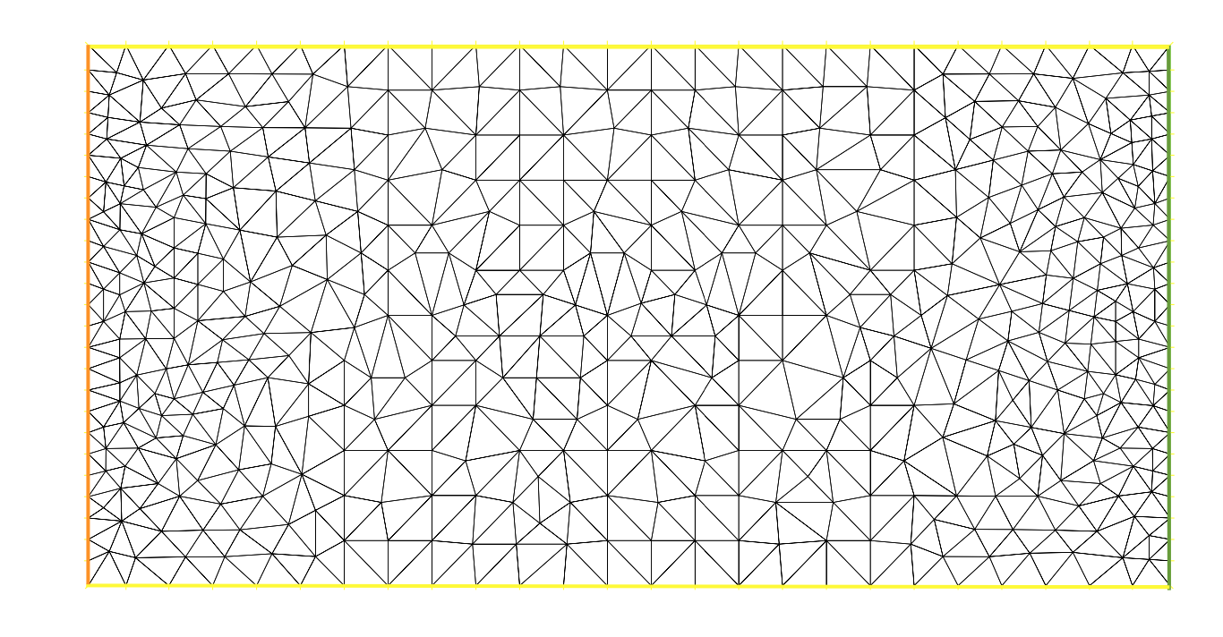
Figure 1: The domain and the “Standard Mesh”; $\Omega$ is composed by $\Gamma_{in}$, on the left side, $\Gamma_{out}$ on the right side and the others walls are $\Gamma_{\omega}$. Number of nodes: 535 . Number of triangles: 968.

In the first experiment, we initialized the control as $g^{0}=0.9\cdot u^{0}$, in a relatively small neighborhood of the Dirichlet condition that provided $u_{d}$.

The stopping criteria for ALG 1 and ALG 2 was

$$\frac{\|u^{n}-u_{d}\|_{L^{2}((0,T)\times\Omega)}}{\|u_{d}\|_{L^{2}((0,T)\times\Omega)}}\leq\varepsilon\quad\mbox{ and }\quad\frac{\|u^{n}(T)-\tilde{u}_{d}\|_{L^{2}(\Omega)}}{\|\tilde{u}_{d}\|_{L^{2}(\Omega)}}\leq\varepsilon$$

with $\varepsilon=0.05$.

In order to compare both algorithms we present several results in Figure 2. Specifically, we compare the number of iterations required for the stopping criteria to be fulfilled, for two pairs of parameters, and for different values for the Reynolds number $Re$.

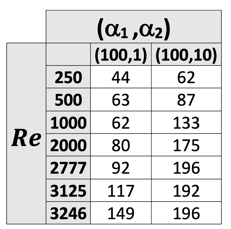
(a) ALG 1

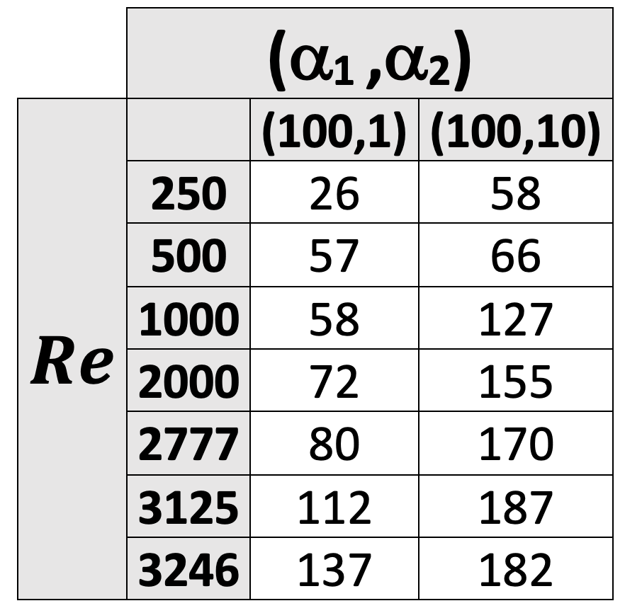
(b) ALG 2

Figure 2: Iterates number carried out to solve the problem with the two algorithms for various $Re$ and for the given two pairs of parameters $\alpha_{1}$ and $\alpha_{2}$, ($\alpha_{3}=10^{-3}$).

Observe that, in these experiments, ALG 2 tends to require fewer iterations to fulfill the stopping criteria. Concerning the Reynolds number, we can see that, as it increases, also the number of the minimization iterates required grows. Note also that when we increase $\alpha_{2}$ from $1$ to $10$ (fixing $\alpha_{1}$ and $\alpha_{3}$), the number of iterations to fulfill the stopping criteria increases as well. If not mentioned differently, in what follows, we present the results for $\alpha_{1}=100$, $\alpha_{2}=1$ and $\alpha_{3}=10^{-3}$.

In what follows, we perform a second set of experiments with a finer mesh (see Figure 3), which we called “Fine Mesh”. Besides, we run the simulations on both meshes using also a time step one order smaller $dt=0.02$. We fixed a sufficiently large $Re=1000$, for the convective effects to be relevant. For a comparison of the required number of iterations for both meshes and time steps, see the table in Figure 4. We observe that the number of iterations increases considerably when refining the mesh and the time step (with a much greater influence of the time step). The final cost function’s value (see Figures 5.c and 6.c) is considerably lower for the refined time step. In particular, the finer time grid allows a substantial reduction of $J_{2}$ which measures the fitting at the final time (see Figures 5.b and 6.b).

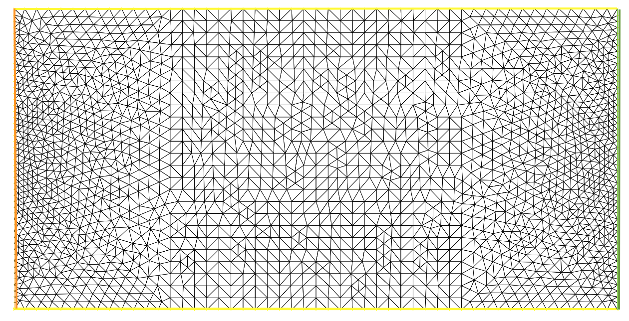
Figure 3: The domain and the “Fine Mesh”; $\Omega$ is composed by $\Gamma_{in}$, on the left side, $\Gamma_{out}$ on the right side and the others walls are $\Gamma_{\omega}$. Number of nodes: 2114. Number of triangles: 4026.

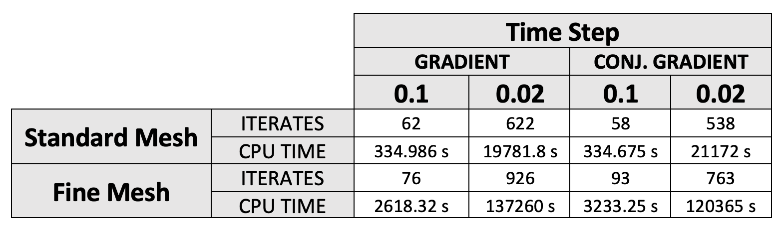
Figure 4: Computation times (in seconds) and numbers of iterates to reach an error smaller than $\varepsilon=0.05$ for $Re=1000$, $\alpha_{1}=100$, $\alpha_{2}=1$ and $\alpha_{3}=10^{-3}$.

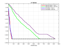
(a) $J_{1}$ Relative errors

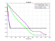
(b) $J_{2}$ Relative errors

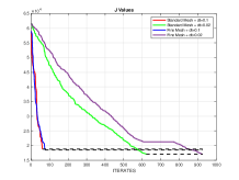
(c) $J$ Values

Figure 5: Functional value and relative error for different initials controls with ALG 1 and $Re=1000$, $\alpha_{1}=100$, $\alpha_{2}=1$ and $\alpha_{3}=10^{-3}$.

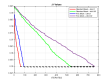
(a) $J_{1}$ Relative errors

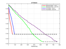
(b) $J_{2}$ Relative errors

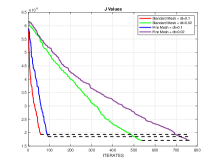
(c) $J$ Values

Figure 6: Functional value and relative error for different initials controls with ALG 2 and $Re=1000$, $\alpha_{1}=100$, $\alpha_{2}=1$ and $\alpha_{3}=10^{-3}$.

In a third set of experiments, we initiated ALG 1 using $g^{0}=0.8\cdot u_{0}$ and $g^{0}=0.7\cdot u_{0}$, which corresponds to initial states with global errors of around $25\%$ and $30\%$ respectively. We changed the parameter in the stopping criteria $\varepsilon$ to $\varepsilon=0.1$.

Looking at Figure 7, we can see a comparison between these experiments and the previous ones, obtained with $g^{0}=0.9\cdot u_{0}$. It can be seen that, the further away the algorithm starts, the harder it becomes to fit the desired state. Even so, the distance can be substantially reduced. In our experiments, we have also detected that the weight of the parameters is important when solving the problem and the difficulty of it depends directly on the size of the mentioned weights. The selection here presented for the weighting parameters was among the best options experimentally tested.

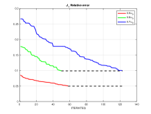
(a) $J_{1}$ Relative errors

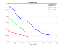
(b) $J_{2}$ Relative errors

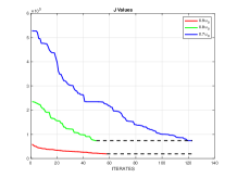
(c) $J$ Values

Figure 7: Functional value for ALG 1 and relative error for different initials controls with $Re=1000$, $\alpha_{1}=100$, $\alpha_{2}=1$ and $\alpha_{3}=10^{-3}$.

Next, we present the results for the optimal solution obtained with a constant initial control is $g^{0}=16.667$. This value corresponds to the average velocity of the parabolic profile used to generate $u_{d}$.

The weighting parameters were fixed as before ($\alpha_{1}=100,$ $\alpha_{2}=1$ and $\alpha_{3}=10^{-3}$). We used firstly ALG 1 and after ALG 2 on the Standard Mesh but, this time, the stopping criteria was chosen to be:

$$\frac{\|u^{n}-u_{d}\|_{L^{2}((0,T)\times\Omega)}}{\|u_{d}\|_{L^{2}((0,T)\times\Omega)}}\leq 0.05\quad\mbox{ and }\quad\frac{\|u^{n}(T)-\tilde{u}_{d}\|_{L^{2}(\Omega)}}{\|\tilde{u}_{d}\|_{L^{2}(\Omega)}}\leq 0.1$$

For ALG 1 and $Re=500$, the stopping criteria was fulfilled after $1195$ iterations and a CPU time of $6994.18$. In Figure 8, we compare the relative error functionals and the functional values, along the iterative process, for the optimal solutions obtained with the initial parabolic guess (as in Test 1) and the optimal solution obtained with the constant average flow as the initial estimate. We distinguish between both results referring to ”Parabolic control” and “Constant control”, respectively.

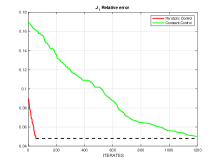
(a) $J_{1}$ Relative errors

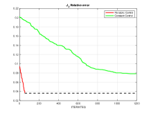
(b) $J_{2}$ Relative errors

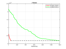
(c) $J$ Values

Figure 8: Relative error with ALG 1, $Re=500$, $\alpha_{1}=100$, $\alpha_{2}=1$ and $\alpha_{3}=10^{-3}$.

In Figure 9, we also present the results for a higher Reynolds number ($Re=1000$) with ALG 2. The stopping criteria was fulfilled after $1472$ iterations and with a CPU time of $9415.74$ s.

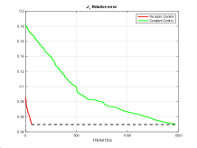
(a) $J_{1}$ Relative errors

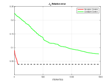
(b) $J_{2}$ Relative errors

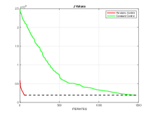
(c) $J$ Values

Figure 9: Relative error with ALG 2, $Re=1000$, $\alpha_{1}=100$, $\alpha_{2}=1$ and $\alpha_{3}=10^{-3}$.

As we can see, in both cases the error functionals are significantly reduced. However, the time and number of iterations required for the constant initial control were larger than for the parabolic control. This is what was expected as the constant control requires more significant transformations in order to minimize the fitting functional.

Finally, we addressed the case when the desired state was not a solution of the Navier-Stokes equations, but a noisy perturbation of such a solution. To this purpose, we added to $u_{d}$ computed as above, a random error (between $0$ and $1$) in each component. This corresponds to a signal to noise ratio of $0.05$. Next, we use ALG 1 with initial estimate given by $g^{0}=0.9\cdot u^{0}$, where $u^{0}=(y\cdot(10-y),0)$ was the steady parabolic profile. We used the Standard Mesh and a time step $dt=0.1$.

The stopping criteria was defined as above, but taking $\varepsilon=0.055$ in order to keep the relative error above the signal to noise ratio. It took $195$ iterations for this criteria to be fulfilled. In Figure 10, we compare the evolution of the cost function value and relative errors for the ”noisy” case as well as the ”noisy free” case. We identify the later as the ”Parabolic Control Solution”.

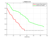
(a) $J_{1}$ Relative errors

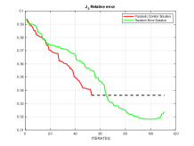
(b) $J_{2}$ Relative errors

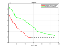
(c) $J$ Values

Figure 10: Relative error with $Re=500$, $\alpha_{1}=100$, $\alpha_{2}=1$ and $\alpha_{3}=10^{-3}$.

In this case, we can observe that the algorithm obtains a good approximation of the solution as in the case that we have a good desired state solution to the Navier-Stokes equations. However we want to highlight the value of the stop test $\varepsilon$ because it cannot be so low as in the parabolic control due to the noise ratio.

Test 2: Time dependent data

This test was performed considering time-dependent data. To this end, we manufactured $u_{d}$ by solving the NS (3) again with $f=0$, but taking the Dirichlet data to be a time-dependent parabolic profile given by

$$g=(1+t)\cdot u^{0}\text{, with }u^{0}=(y\cdot(10-y),0)$$

and the total stress fixed at

$$h=((1+t)\cdot(2x-40),(1+t)\cdot(10-2y)).$$

The stopping criteria for ALG 1 and ALG 2 was

$$\frac{\|u^{n}-u_{d}\|_{L^{2}((0,T)\times\Omega)}}{\|u_{d}\|_{L^{2}((0,T)\times\Omega)}}\leq\varepsilon\quad\mbox{ and }\quad\frac{\|u^{n}(T)-\tilde{u}_{d}\|_{L^{2}(\Omega)}}{\|\tilde{u}_{d}\|_{L^{2}(\Omega)}}\leq\varepsilon$$

with $\varepsilon=0.05$.

In order to compare the behavior of the Gradient and the Conjugate Gradient algorithms, we present in Figure 11 the numbers of iterates needed by each method to fulfill the stopping criteria.

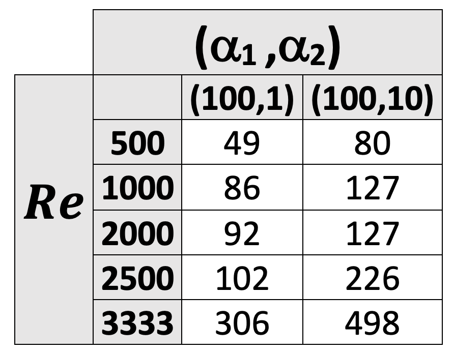
(a) ALG 1

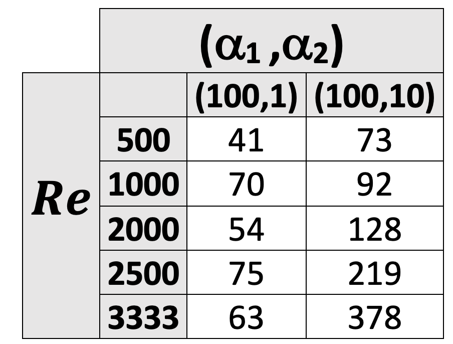
(b) ALG 2

Figure 11: The final velocity fields computed for various $Re$ and various $\alpha_{1}$ and $\alpha_{2}$, ($\alpha_{3}=10^{-3}$).

In this case, we observe a similar pattern, in terms of convergence, as with the stationary data. Again, additional iterations are required when higher Reynolds numbers are considered.

Test 3: 2D stenotic vessel

Our final test addressed an idealized domain representing a partially obstructed vessel.

The domain $\Omega$ is represented in Figure 12. As in the previous case, the left side is the inlet boundary (where we imposed the control) while the right side corresponds to outlet boundary (where we imposed the total stress condition). The remaining boundaries represent the vessel wall where we imposed homogeneous Dirichlet conditions.

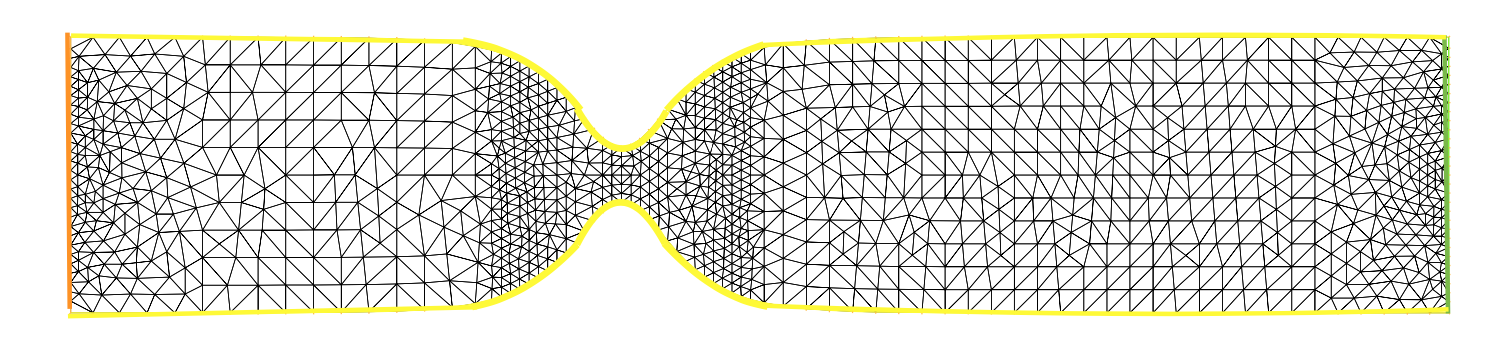
Figure 12: The domain $\Omega$ and the mesh; $\partial\Omega$ is composed of $\Gamma_{in}$ (the left side), $\Gamma_{out}$ (the right side) and $\Gamma_{\omega}$ (the remaining of boundary).

We want to drive the solution close to desired states, $u_{d}(t,x)$ and $\tilde{u}_{d}(x)=u_{d}(x,T)$, where $u_{d}$ is a noisy perturbation of the solution of (24), and $T=1$:

$$\left\{\begin{array}[]{llllll}\displaystyle\partial_{t}u-\nabla\cdot(2\nu D(u))+\frac{1}{2}\nabla|u|^{2}+(\nabla\times u)\times u+\nabla p=0&\quad(0,T)\times\Omega,\\ \nabla\cdot u=0&\quad(0,T)\times\Omega,\\ u=(1.5t\cdot y\cdot(2-y),0)&\quad(0,T)\times\Gamma_{in},\\ u=0&\quad(0,T)\times\Gamma_{\omega},\\ \Big{(}2\nu D(u)-(p+\frac{1}{2}|u|^{2})I\Big{)}\cdot\overline{n}=(0,0)&\quad(0,T)\times\Gamma_{out},\\ u(0,x)=(0,0)&\quad\Omega\end{array}\right.$$ (24)

Again, we set the goal of minimizing (9) subject to (3), fixing $f$, $h$ and $u_{0}$ as in (24), but letting $g$ as the unknown variable. For that purpose we relied on ALG 1 applied to the mesh depicted in Figure 12. For the space discretization we used the P2 - P1 FEM approximation and we considered a time step of $dt=0.1$.

The stopping criteria for the Gradient algorithm (ALG 1) was

$$\frac{\|u^{n}-u_{d}\|_{L^{2}((0,T)\times\Omega)}}{\|u_{d}\|_{L^{2}((0,T)\times\Omega)}}\leq\varepsilon\quad\mbox{ and }\quad\frac{\|u^{n}(T)-\tilde{u}_{d}\|_{L^{2}(\Omega)}}{\|\tilde{u}_{d}\|_{L^{2}(\Omega)}}\leq\varepsilon$$

with $\varepsilon=0.05$.

We considered, as intial guess for the control,

$$g^{0}=1.5\displaystyle\sin(\frac{\pi}{2}t)\cdot y\cdot(2-y).$$

It took $514$ iterates and a CPU time of $3696.76$ s to achieve the stopping criteria. The results can be seen in Figure 13. The noisy velocity profiles $u_{d}$ are represented for several snapshots on the left column. The approximation of the optimal solution is depicted on the right column. For the evolution of the relative errors with respect to $u_{d}$ and $u_{d}(T,.)$, as well as the cost functional values, see Figure 14 on the left and on the right, respectively. The solution of (24) is characterized by a maximum $Re=2200$. In Figure 14.a we can see that the relative error of the corresponding velocity is reduced from more than $25\%$ to $5\%$.

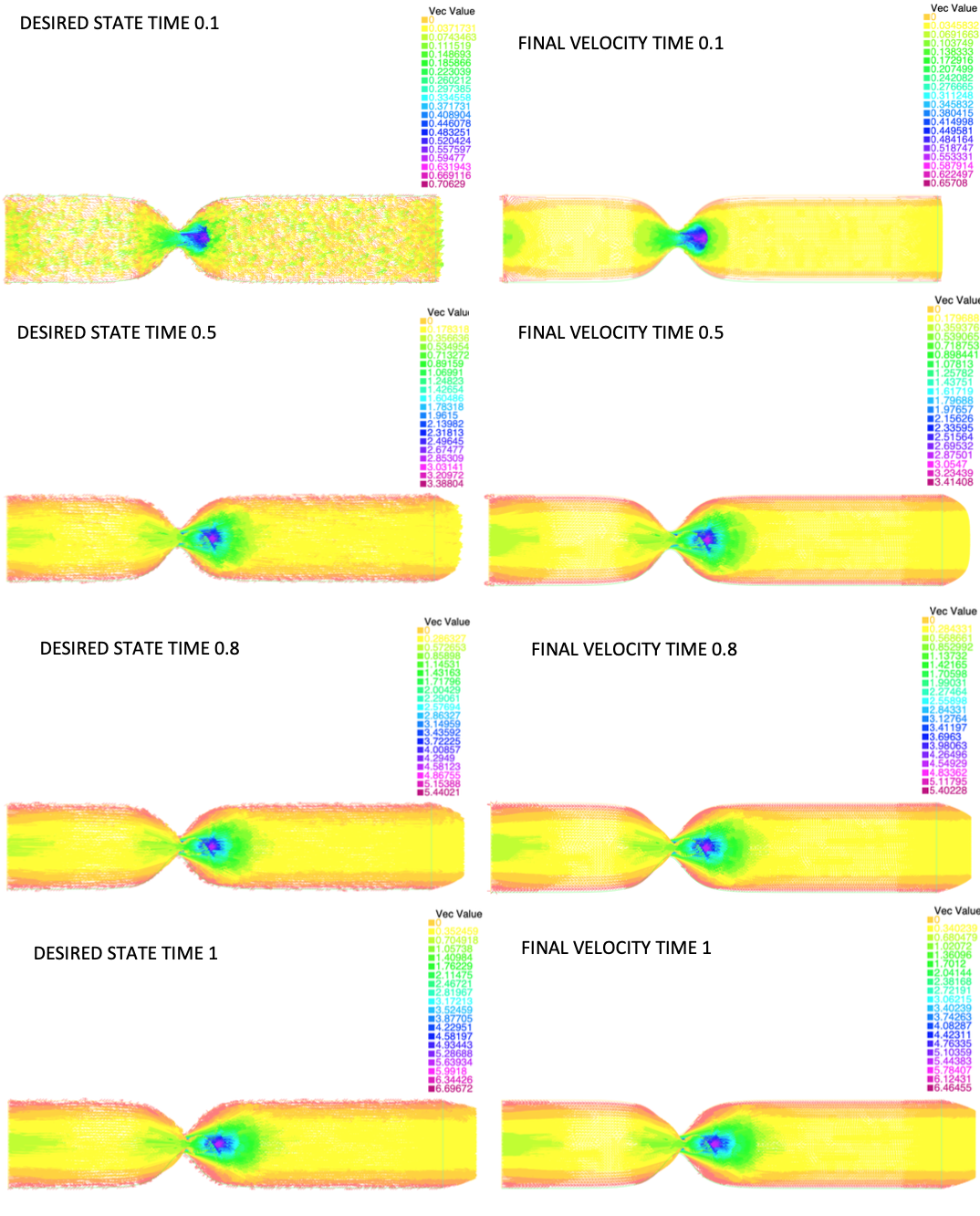
Figure 13: The final velocity fields computed with ALG 1, for $Re=2200$, $\alpha_{1}=100$, $\alpha_{2}=1$ and $\alpha_{3}=10^{-3}$.

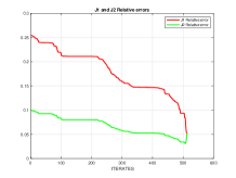
(a) $J_{1}$ and $J_{2}$ Relative errors

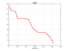
(b) $J$ Values

Figure 14: Relative error with $Re=2200$, $\alpha_{1}=100$, $\alpha_{2}=1$ and $\alpha_{3}=10^{-3}$.

Finally, we tested the response of the minimization algorithm with respect to changes in Reynolds number. We chose to present the results for the largest value $Re=5100$. In this case, the data was obtained by adding noise to solution of (24), as before, but using the expression $g=(4t\cdot y\cdot(2-y),0)$ as Dirichlet boundary data.

We initiate the algorithm with $g^{0}=4\displaystyle\sin(\frac{\pi}{2}t)\cdot y\cdot(2-y)$. The relative error of the corresponding velocity with respect to the noisy data is higher than $27\%$ (see J1 relative error at iterate zero in Figure 16.a).

It took $1147$ iterates and $7094.8$ s of CPU time to fulfill the stopping criteria. In Figure 15 we can see the noisy data on the left and the optimal solution on the right. Notice the presence of recirculations after the stenosis. In Figure 16 we can see that number required iterates increases but the initial error is strongly reduced.

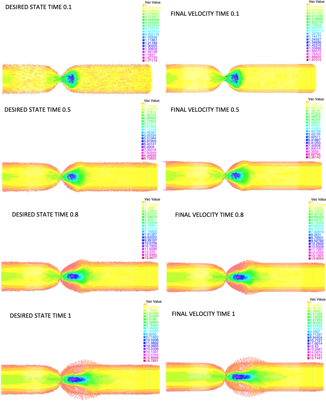
Figure 15: The final velocity fields computed with ALG 1, for $Re=5100$, $\alpha_{1}=100$, $\alpha_{2}=1$ and $\alpha_{3}=10^{-3}$.

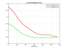
(a) $J_{1}$ and $J_{2}$ Relative errors

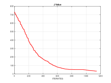
(b) $J$ Values

Figure 16: Relative error with $Re=5100$, $\alpha_{1}=100$, $\alpha_{2}=1$ and $\alpha_{3}=10^{-3}$.

5 Conclusions

In this work, we have provided necessary conditions for a boundary control problem associated with the time-dependent Navier-Stokes equations, under boundary conditions of mixed type. In a certain sense, it can be seen as an extension of the work performed in [19], to the 2D case, and under mixed boundary conditions. It can also be understood as an extension to the time-dependent case of the work performed in [21]. The analysis of the reduced cost also provided us the tools to define descent-type algorithms such as the gradient and conjugate gradient algorithms. Using a FEM approximation, we could see that an initial guess, associated with a relative error greater than $25\%$ in the fitting term, can be improved until decreasing the relative fitting error to less than $5\%.$ This is the case, even when high Reynolds numbers are considered, as well as nonphysical data.

One of the major contributions of this work is to lay the groundwork for extending it to the three-dimensional case. It is important to note that this extension is by no means trivial, and we are currently working on it. One of the key aspects to consider in the three-dimensional case is that in this situation we do not have uniqueness of solution nor good regularity even with Dirichlet-type conditions. Therefore, in the three-dimensional case, it will be necessary to work under the assumption that a unique solution exists and assuming sufficient regularity to demonstrate similar results to those presented in this work. Additionally, since gradient-type algorithms are known to become computationally expensive, parameterized approaches are now being considered for 3D simulations. Future extensions may consider non-Newtonian or compressible assumptions, as well as multiple boundary controls.

Statements and Declarations

• Funding

  The authors were partially supported by Fundação para a Ciência e Tecnologia through the research project PTDC/MAT-APL/7076/2020 DOI (https://doi.org/10.54499/PTDC/MAT-APL/7076/2020) and the CEMAT’s research project UIDB/04621/2020/IST-ID (DOI: https://doi.org/10.54499/UIDB/04621/2020).

• Conflict of interest/Competing interests

  The authors have no relevant financial or non-financial interests to disclose.

References

- [1] J. Bernard, Time-dependent Stokes and Navier–Stokes problems with boundary conditions involving pressure, existence and regularity, Nonlinear Analysis-real World Applications - NONLINEAR ANAL-REAL WORLD APP 4 (2003), 805–839, doi: 10.1016/S1468-1218(03)00016-6.
- [2] M. Delia, M. Perego, and A. Veneziani, A Variational Data Assimilation Procedure for the Incompressible Navier-Stokes Equations in Hemodynamics, Journal of Scientific Computing 52(2) (2011), 340–359.
- [3] E. Fernández-Cara and I. Marín-Gayte, Theoretical and numerical bi-objective optimal control: Nash equilibria, ESAIM Control Optim. Calc. Var. 27 (2021), 50.
- [4] E. Fernández-Cara and I. Marín-Gayte, Theoretical and numerical results for some bi-objective optimal control problems, Communications on Pure and Applied Analysis 19(4) (2020), 2110–2126.
- [5] S.W. Funke, M. Nordaas, O. Evju, M.S. Alnaes, and K.A. Mardal, Variational data assimilation for transient blood flow simulations: cerebral aneurysms as an illustrative example, Int J Numer Method Biomed Eng 35 (2019), e3152.
- [6] L. Formaggia, A. Moura, and F. Nobile, On the stability of the coupling of 3D and 1D fluid-structure interaction models for blood flow simulations, ESAIM: Mathematical Modelling and Numerical Analysis - Modélisation Mathématique et Analyse Numérique 41(4) (2007), 743–769.
- [7] A. V. Fursikov (ed.), Optimal Control of Distributed Systems: Theory and Applications, American Mathematical Society, Boston, MA, USA, 2000.
- [8] A. V. Fursikov, M. D. Gunzburger, and L. Hou, Optimal boundary control for the evolutionary Navier–Stokes system: The three-dimensional case, SIAM J Control Optim 43 (2005), 2191–2232.
- [9] A. V. Fursikov and R. Rannacher (eds.), Optimal Neumann Control for the Two-Dimensional Steady-State Navier-Stokes Equations, Editors, New Directions in Mathematical Fluid Mechanics: The Alexander V. Kazhikhov Memorial Volume, Basel: Birkhauser, 2010.
- [10] R. Glowinski (ed.), Finite Element Methods for Incompressible Viscous Flow, Handbook of Numerical Analysis, 9, Amsterdam, 2003.
- [11] T. Guerra, A. Sequeira, and J. Tiago, Existence of optimal boundary control for the Navier-Stokes equations with mixed boundary conditions, Port Math 72 (2015), 267–283.
- [12] T. Guerra, C. Catarino, T. Mestre, S. Santos, J. Tiago, and A. Sequeira, A data assimilation approach for non-Newtonian blood flow simulations in 3D geometries, Applied Mathematics and Computation 321 (2018), 176–194.
- [13] M. D. Gunzburger (ed.), Flow Control, Springer-Verlag, New York, 1995.
- [14] M. D. Gunzburger, L. Hou, and T.P. Svobodny, Boundary velocity control of incompressible flow with an application to viscous drag reduction, SIAM J Control Optim 30 (1992), 167–181.
- [15] M. D. Gunzburger, L. Hou, and T.P. Svobodny, Analysis and finite element approximation of optimal control problems for the stationary Navier-Stokes equations with Dirichlet controls, ESAIM: Math Model Numer Anal 25 (1991), 711–748.
- [16] M. D. Gunzburger and S. Manservisi, The velocity tracking problem for Navier-Stokes flows with boundary control, SIAM J Control Optim 39 (2000), 594–634.
- [17] F. Hecht, http://www.freefem.org.
- [18] J.G. Heywood, R. Rannacher, and S. Turek, Artificial boundaries and flux and pressure conditions for the incompressible Navier–Stokes equations, Int. J. Numer. Meth. Fluids 22 (1996), 325–352.
- [19] M. Hinze and K. Kunisch, Second order methods for boundary control of the instationary Navier‐Stokes system, ZAMM‐Journal of Applied Mathematics and Mechanics, Applied Mathematics and Mechanics 84(3) (2004), 171–187.
- [20] H. Kim, A boundary control problem for vorticity minimization in time-dependent 2D Navier-Stokes equations, Korean J Math 23 (2006), 293–312.
- [21] A. Manzoni, A. Quarteroni, and S. Salsa, A saddle point approach to an optimal boundary control problem for steady Navier-Stokes equations, Mathematics in Engineering 1(2) (2019), 252–280.
- [22] A. Manzoni, A. Quarteroni, and S. Salsa (eds.), Optimal Control of Partial Differential Equations, Applied Mathematical Sciences, Springer, Cham, 2021.
- [23] S. Sritharan (ed.), Optimal Control of Viscous Flow, SIAM, Philadelphia, 1998.
- [24] R. Temam (ed.), Navier-Stokes equations. Theory and numerical analysis, Studies in Mathematics and Applications,