A primary quantum current standard based on the Josephson and the quantum Hall effects

Abstract

The new definition of the ampere calls for a quantum current standard able to deliver a flow of elementary charges per second controlled with a relative uncertainty of one part in $10^{8}$. Despite many efforts, nanodevices handling electrons one by one have never been able to demonstrate such an accuracy. The alternative route based on applying Ohm’s law to the Josephson voltage and quantum Hall standards recently reached the target uncertainty but this was at the expense of the application of error corrections, hampering simplicity and further improvement. As a result, national metrology institutes still lack an operational quantum current standard. Here, we present a new quantum current generator, combining both quantum standards and a superconducting cryogenic amplifier, free of error correction, which provides quantized currents driven by the Josephson microwave signal. We show that it can realize the ampere definition with the target uncertainty over a range extended from mA down to $\mu$A and improve end-user current measurements, which are up to now a hundred times less accurate. Other prospects include measuring large resistances using the new current standard in conjunction with a quantum voltmeter and, by exploiting its low-noise performances, bridging the gap with the lower currents of other quantum current sources.

Since the last revision of the International System of Units (SI) in May 20, 2019, founded on seven fixed constants of natureBIPM (9th edition, 2019); Poirier et al. (2019), any source generating an electric current which can be expressed in terms of $ef$, with $e$ the elementary charge and $f$ a frequency in Hz ($\mathrm{s^{-1}}$), provides a realisation of the ampere.

Single-electron current sources (SECS) Pothier et al. (1992); Pekola et al. (2013); Scherer and Schumacher (2019), which are mesoscopic devices Keller et al. (1999); Pekola et al. (2008); Camarota et al. (2012); Giblin et al. (2012); Stein et al. (2015, 2017); Yamahata et al. (2016); Zhao et al. (2017); Bae et al. (2020), able to handle electrons one by one at a rate $f_{e}$, are often presented as the most obvious way to realize the definition. However, achieving currents above 100 pA using GaAs and Si-based tunable-barrier SECS accurate to within a relative uncertainty better than $10^{-7}$ remains a very challenging goal because of increasing error rates at high frequencies ($\sim$ 1 GHz) Kataoka et al. (2011); Ahn et al. (2017). Very recently, as a consequence of the phase-charge quantum mechanical duality in Josephson junctions (JJ), dual Shapiro steps have been evidenced in superconducting nanowires and small JJ placed in high impedance environments under microwave radiation Shaikhaidarov et al. (2022); Crescini et al. (2023); F. Kaap and Lotkhov . Here, the enhanced phase variance allows photon-assisted tunneling of fluxons $\phi_{0}=h/2e$ ($h$ is the Planck constant) and a synchronized transfer of Cooper pairs. Sharp current steps appearing at integer multiples of $2ef_{e}$ in the DC current-voltage characteristics could be promising candidates as quantum sources in the nA range, although their flatness is still in debate Kurilovich et al. (2024). More generally, for all mesoscopic current sources, the control of charge fluctuations, which are dependent on the device coupling with the electromagnetic environment, remains a crucial issue.

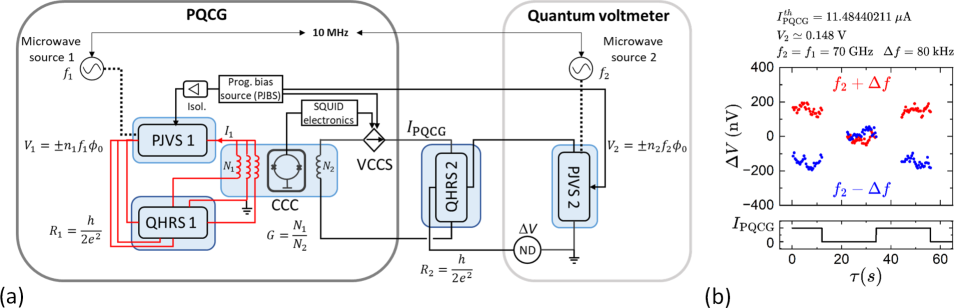
Figure 1: Experimental set-up for the accuracy test of the PQCG. (a) The PQCG is composed of $\mathrm{PJVS_{1}}$ and $\mathrm{QHRS_{1}}$ connected through a triple connection (red lines) ensured via the windings of $N_{1}$ turns of a new CCC, which are used to measure and amplify the quantized current $I_{1}$. The shields at ground potential of the high and low potential cables are not shown on the scheme. The SQUID detector of the CCC feedbacks on an external current source (VCCS) which maintains the current $I_{\mathrm{PQCG}}$ into the series connection of $\mathrm{QHRS_{2}}$ and of the winding of $N_{2}$ turns. To reduce the finite gain error of the SQUID, a voltage source of the programmable Josephson bias source (PJBS) drives the VCCS and preadjusts the output current, such that the SQUID feedbacks only on a small fraction of $I_{\mathrm{PQCG}}$ (Methods). The voltage drop at $\mathrm{QHRS_{2}}$ is measured in a quantum voltmeter configuration made of $\mathrm{PJVS_{2}}$ and a null detector, ND (EMN11 from EM electronics). The frequency of the Josephson microwave signals are referenced to a 10 MHz frequency standard linked to an atomic clock time base. Both PJVS are controlled and synchronized using the same PJBS. A decoupling stage ensures the electrical isolation between the two PJVS (except for the accuracy test done with $n_{1}=1920$ (Methods)) so that the PQCG and the quantum voltmeter can be both referenced at separate grounding points. (b) ND recordings, $\Delta V$, for frequencies $f_{2}+\Delta f$ and $f_{2}-\Delta f$ as a function of time $\tau$ while the current $I_{\mathrm{PQCG}}$ is periodically switching on and off (I₊ measurement protocol).

Concurrently, another route to the SI realization consists in applying Ohm’s law to the Josephson voltage and quantum Hall resistance standards, since the Josephson effect Josephson (1962) and the quantum Hall effect von Klitzing et al. (1980) now provide direct and universal realizations of the volt and the ohm from $h/2e$ and $h/e^{2}$ constants, respectively Poirier et al. (2019), with a $10^{-9}$ measurement uncertainty. The high accuracy of the Josephson voltage standards, which are series arrays of JJ, relies on the phase rigidity of macroscopic superconductors. Under application of dc current bias and a microwave radiation $f_{\mathrm{J}}$, the transfer through each JJ of one fluxon per period of the microwave tone is ensured and results in a quantized voltage $V=n_{\mathrm{J}}\phi_{0}f_{\mathrm{J}}$ Shapiro (1963), where $n_{\mathrm{J}}$ is the number of JJ. If this quantized voltage can be accurately applied to a quantum Hall resistance standard (QHRS) in the $\nu$=2 Landau level filling factor, taking advantage of the charge rigidity of the quantum Hall edge states, $n_{\mathrm{J}}e$ charges are transferred at a rate $f_{\mathrm{J}}$ through the QHRS of $h/2e^{2}$ resistance. Hence, a current $n_{\mathrm{J}}ef_{\mathrm{J}}$, easily reaching microamperes, can be generated. Recently, a calculable current of 1 $\mu$A generated from the series connection of both quantum standards has been measured with a relative uncertainty of $1.3\times 10^{-7}$ Chae et al. (2022); Kaneko et al. (2024), but the accuracy was reached owing to the very low-resistance of the ammeter ($\sim 0.1$ m$\Omega$). The main issue is therefore to implement the accurate series connection of the two quantum standards while realizing a true current source. The programmable quantum current generator (PQCG) Poirier et al. (2014); Brun-Picard et al. (2016); Djordjevic et al. (2021) has addressed this issue by locking an electron flow to the current circulating in the loop formed by the quantum standards, with the help of a superconducting amplifier, allowing simultaneously the scaling over a wider range of current values. Its accuracy was demonstrated in the mA range with a relative measurement uncertainty of $10^{-8}$. This result was however obtained at the expense of corrections of the order of a few parts in $10^{7}$ and of several time-consuming calibrations, impairing the final uncertainty and the full potential of the new quantum current standard.

Here, we implement a next-generation PQCG operating without any classical correction and with a lower noise level. We demonstrate the realization of the ampere with relative uncertainties below $10^{-8}$ for different current levels filling the gap between the mA range and the $\mu$A range using a full quantum instrumentation implying five quantum devices.

Next-generation PQCG
Fig.1a shows the implementation (Methods) of two programmable Josephson voltage standards (PJVS), two QHRS and a cryogenic current comparator (CCC). The two PJVS are binary divided 1 V $\mathrm{Nb/Nb_{x}Si_{1-x}/Nb}$ series arrays Behr et al. (2012), both having a total of 8192 JJ and working around 70 GHz. The voltage of the two PJVS are given by $\pm n_{1,2}\phi_{0}f_{\mathrm{1,2}}$ with $n_{1,2}$ the number of JJ biased on the $\pm$1 Shapiro steps. The two QHRS are both GaAs/AlGaAs heterostructures Piquemal et al. (1993) of quantized resistance $R_{1}=R_{2}=h/2e^{2}$. The CCC is a dc current transformerHarvey (1972), made of several superconducting windings of different number of turns, able to compare currents with a great accuracy (below one part in $10^{9}$) and sensitivity (80 pA$\cdot$turns/$\mathrm{Hz^{1/2}}$) owing to Ampère’s theorem and Meissner effect.

The new version of the PQCG is composed of $\mathrm{PJVS_{1}}$ Behr et al. (2012) connected to $\mathrm{QHRS_{1}}$ with a triple connection (Extended Data fig.1) ensured through three identical windings of $N_{1}$ turns of a new specially designed CCC (see Extended Data fig.2 and Methods). This connection technique Delahaye (1993) reduces the impact of the series resistances to an insignificant effect. More precisely, one current contact and two voltage contacts of the same equipotential of $\mathrm{QHRS_{1}}$ are connected all together at each superconducting pads of $\mathrm{PJVS_{1}}$. Because of the topological properties of Hall edge-states, namely their chirality, their $h/e^{2}$ two-wire resistance and their immunity against backscattering Buttiker (1988), the current flowing through the third contact is only a fraction $(r/R_{1})^{2}$ of the current circulating in the first one, where $r$ is the typical resistance of the connections. The resistance seen by $\mathrm{PJVS_{1}}$ is close to $h/2e^{2}$ within a typical small correction of order $(r/R_{1})^{3}$. It results that the total current circulating $I_{1}$, is close to $\pm n_{\mathrm{1}}ef_{1}$ within 1.5 parts in $10^{10}$ for series resistance values lower than 5 ohms (Methods). Compared to Brun-Picard et al. (2016), where the double connection required the application of a relative correction to the current of a few $10^{-7}$, the operation of the PQCG is simplified since no correction is necessary here. The quantized current $I_{1}$, divided in the three connections, is measured by the three identical windings of $N_{1}$ turns. A DC SQUID is used to detect the unbalance ampere$\cdot$turns in the different windings of the new CCC. It feedbacks on the new battery-powered voltage controlled current source (VCCS), which supplies a winding of $N_{2}$ turns in order to maintain the ampere$\cdot$turns balance $N_{\mathrm{1}}I_{\mathrm{1}}-N_{\mathrm{2}}I_{\mathrm{PQCG}}=0$. It results that the PQCG is able to output a current equal to:

$$I_{\mathrm{PQCG}}^{th}=\pm(N_{\mathrm{1}}/N_{\mathrm{2}})n_{\mathrm{1}}ef_{\mathrm{1}}$$ (1)

to within a Type B relative uncertainty of 2 parts in $10^{9}$ (Extended Data Table 1). In practice, the CCC gain $G=N_{1}/N_{2}$ can span two orders of magnitude on either side of the unity, allowing the generation of currents from nA to mA.

Accuracy test principle
The accuracy of the quantized current $I_{\mathrm{PQCG}}$ is tested by feeding $\mathrm{QHRS_{2}}$, and by measuring the voltage drop, $V_{2}$, at its Hall terminals using a quantum voltmeter (Extended Data fig.3) made of $\mathrm{PJVS_{2}}$ and an analog null detector (ND), which measures the voltage difference $\Delta V$. From Kirchhoff’s voltage law, $I_{\mathrm{PQCG}}$ is determined according to the expression :

$$V_{2}=R_{\mathrm{2}}I_{\mathrm{PQCG}}=\pm\phi_{0}n_{\mathrm{2}}f_{\mathrm{2}}-\Delta V,$$ (2)

with $\Delta V=0$ ideally at the equilibrium frequency $f_{\mathrm{2}}^{eq}$. Using a quantized resistance, $R_{\mathrm{2}}=h/2e^{2}$ ($\sim 12.9~{}\mathrm{k}\Omega$), about 129 times higher than in Brun-Picard et al. (2016) allows increasing the signal-to-noise ratio while eliminating an extra resistance calibration. The relative deviation of the measured current to the theoretical one, $\Delta I/I=(I_{\mathrm{PQCG}}/I_{\mathrm{PQCG}}^{th})-1$, is given by $\Delta I/I=\frac{n_{\mathrm{2}}f_{\mathrm{2}}^{eq}}{Gn_{\mathrm{1}}f_{\mathrm{1}}}-1$. In practice, the CCC gain and the numbers of JJ are chosen so that $Gn_{\mathrm{1}}=n_{\mathrm{2}}$. Thus, the nominal relative deviation is given by:

$$\Delta I/I=\frac{f_{\mathrm{2}}^{eq}}{f_{\mathrm{1}}}-1$$ (3)

The accuracy test therefore resumes to the determination of a frequency ratio close to one. However, noise and offset drifts prevents from finding the frequency $f_{\mathrm{2}}^{eq}$ setting $\Delta V=0$ accurately. Two successive voltage mean values, $\overline{\Delta V_{f_{2}^{+}}}$ and $\overline{\Delta V_{f_{2}^{-}}}$, are rather measured at two different frequencies $f_{\mathrm{2}}^{+}=f_{\mathrm{2}}+\Delta f$ and $f_{\mathrm{2}}^{-}=f_{\mathrm{2}}-\Delta f$ respectively, where $f_{\mathrm{2}}$ is chosen close to $f_{2}^{eq}$ ($\sim f_{\mathrm{1}}$) and $\Delta f$ is set to 40 kHz or 80 kHz in our experiments (fig.1b and Extended Data fig.4a). In order to mitigate the effect of offsets, drifts and 1/$f$ noise, each voltage mean value is obtained from a measurement series consisting in periodically either switching on and off the current with $I_{\mathrm{PQCG}}>0$ (I₊) or $<0$ (I_-), or completely reversing the current (I_±). The equilibrium frequency is then determined from :

$$f_{\mathrm{2}}^{eq}=\frac{f_{\mathrm{2}}^{-}\overline{\Delta V_{f_{2}^{+}}}-f_{\mathrm{2}}^{+}\overline{\Delta V_{f_{2}^{-}}}}{(\overline{\Delta V_{f_{2}^{+}}}-\overline{\Delta V_{f_{2}^{-}}})},$$ (4)

which implies only voltage ratios, relaxing the need to calibrate the gain of the nanovoltmeter. Finally, the determination of $\Delta I/I$ does not require any calibration, resulting in a reduced Type B standard uncertainty, $u^{\mathrm{B}}$, of $2.1\times 10^{-9}$ (Extended Data Table 1). The Type A standard uncertainty of $\Delta I/I$, $u^{\mathrm{A}}=\frac{u^{\mathrm{A}}(f_{\mathrm{2}}^{eq})}{f_{\mathrm{1}}}$ is determined from the standard deviations of the mean of the voltage series $\Delta V_{f_{2}^{+}}$ and $\Delta V_{f_{2}^{-}}$ (Methods).

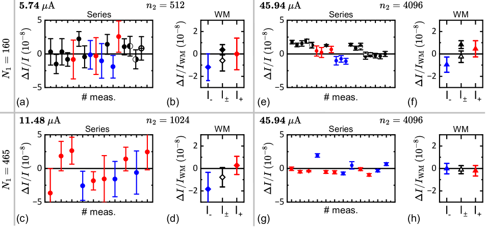
Figure 2: Accuracy tests of the PQCG. Series of relative deviations $\Delta I/I$ with $n_{1}=4096$ measured at 5.742201056 $\mu$A using $N_{1}=160$ (a), at at 11.48440211 $\mu$A using $N_{1}=465$ (c), at 45.93760845 $\mu$A using $N_{1}=160$ (e) and at 45.93760845 $\mu$A using $N_{1}=465$ (g). Measurements were carried out over one or two days, using I₊ ($\tiny{\color[rgb]{1,0,0}\circletfill}$), I_- ($\tiny{\color[rgb]{0,0,1}\circletfill}$) or I_± ($\tiny{\color[rgb]{0,0,0}\circletfill}$) measurement protocols. All uncertainties correspond to one standard deviation, i.e., are given with a coverage factor $k$=1. Error bars correspond to $u^{\mathrm{A}}$. In (a), measurements with $I_{\mathrm{bias}}$ shifted by +0.1 mA ($\tiny{\color[rgb]{0,0,0}\circletfillhl}$) and -0.1 mA ($\tiny{\color[rgb]{0,0,0}\circletfillhr}$), measurement at $f_{\mathrm{1}}=70.02$ GHz ($\tiny{\color[rgb]{0,0,0}\circletlinevh}$). In (e), measurements with $I_{\mathrm{bias}}$ shifted by +0.1 mA ($\tiny{\color[rgb]{0,0,0}\circletfillhl}$) and -0.1 mA ($\tiny{\color[rgb]{0,0,0}\circletfillhr}$), measurements with the double connection and the corresponding $\alpha_{2}=(2.344\pm 0.037)\times 10^{-7}$ correction applied ($\tiny{\color[rgb]{0,0,0}\circletfillha}$), measurements with the triple connection and 50 $\Omega$ inserted into the first connection and the corresponding $\alpha_{3}=(1.4\pm 0.02)\times 10^{-9}$ correction applied ($\tiny{\color[rgb]{0,0,0}\circletfillhb}$). Weighted mean values $\Delta I/I_{\mathrm{WM}}$ of the series measured at 5.74 $\mu$A (b), at 11.48 $\mu$A (d), at 45.94 $\mu$A using $N_{1}=160$ (f) and at 45.94 $\mu$A using $N_{1}=465$ (h). In (b) and (d), weighted mean values for I₊ ($\tiny{\color[rgb]{1,0,0}\rhombusfill}$), I_- ($\tiny{\color[rgb]{0,0,1}\rhombusfill}$), I_± ($\tiny{\color[rgb]{0,0,0}\rhombusfill}$) are calculated from the $u^{\mathrm{A}}$, mean value of I₊ and I_- ($\tiny{\color[rgb]{0,0,0}\rhombus}$). In (f) and (h), weighted mean values for I₊ ($\tiny{\color[rgb]{1,0,0}\trianglepafill}$), I_- ($\tiny{\color[rgb]{0,0,1}\trianglepafill}$), I_± ($\tiny{\color[rgb]{0,0,0}\trianglepafill}$) are calculated from $\sqrt{(u^{\mathrm{A}})^{2}+(u^{\mathrm{A}}_{\mathrm{it-noise}})^{2}}$, where $u^{\mathrm{A}}_{\mathrm{it-noise}}$ accounts for the observed residual intra-day noise, mean value of I₊ and I_- measurements ($\tiny{\color[rgb]{0,0,0}\trianglepa}$). Error bars correspond to combined standard uncertainties $u^{\mathrm{c}}_{\mathrm{WM}}$ (Methods). Other parameter: $N_{2}$ is fixed such as $G=N_{1}/N_{2}=n_{2}/n_{1}$.

Quantized current accuracy
Measurements of $\Delta I/I$ were performed at four different values of current 5.74 $\mu$A, 11.48 $\mu$A, 45.94 $\mu$A and 57.42 $\mu$A, using a primary current $I_{\mathrm{1}}$ of 45.94 $\mu$A obtained with $n_{\mathrm{1}}=4096$. This large current improves the operational margins of the PQCG compared to Brun-Picard et al. (2016) and increases the signal-to-noise ratio while ensuring a perfect quantization of the Hall resistance of the $\mathrm{QHRS_{1}}$ device. Each measurement series was typically carried out over one day using I₊, I_-, and I_± measurement protocols to reveal any systematic effect related to the current direction. Note that implementing complete current reversals I_± required the reduction of the noise in the circuit Djordjevic et al. (2021) (CCC in Methods). Measurements were performed with $N_{1}=160$ or also with $465$ to test the effect of the number of ampere$\cdot$turn. However, the downside of the latter configuration is the higher instability of the feedback loop encountered during the current reversals which prevented the use of the I_± measurement protocol. The different output currents were obtained by changing $N_{2}$ from 80 to 1860. Other PQCG parameters are reported in Extended Data Table 2.

At the lower current values of 5.74 $\mu$A (fig.2a) and 11.48 $\mu$A (fig.2c), discrepancies of $\Delta I/I$ are covered by uncertainties ranging from 1 to $3.10^{-8}$. Weighted means, $\Delta I/I_{\mathrm{WM}}$, for each measurement protocol I₊, I_- and I_±, reported in fig.2b and fig.2d, show that there is no significant deviation of the current from its theoretical value within measurement uncertainties of about $10^{-8}$. Besides, the mean value of $\Delta I/I_{\mathrm{WM}}(\mathrm{I}_{+})$ and $\Delta I/I_{\mathrm{WM}}(\mathrm{I}_{-})$ is clearly in agreement with $\Delta I/I_{\mathrm{WM}}(\mathrm{I}_{\pm})$ at 5.74 $\mu$A, which confirms the equivalence of averaging measurements carried out using the I₊ and I_- protocols with the measurement obtained using the I_± protocol. Combining the different results (Methods), one obtains the relative deviations, for the equivalent protocol I_±, $\overline{\Delta I/I}=(2\pm 4.3)\times 10^{-9}$ and $\overline{\Delta I/I}=(-7.9\pm 8.6)\times 10^{-9}$ at current levels of 5.74 $\mu$A and 11.48 $\mu$A respectively.

At the higher current value of 45.94 $\mu$A, $\Delta I/I$ measurements, reported in fig.2e and fig.2g, are characterized by smaller standard uncertainties in agreement with the larger voltage drop at the terminals of $\mathrm{QHRS_{2}}$ (about 0.59 V). As expected, even smaller uncertainties are observed for $N_{\mathrm{1}}=465$ than for $N_{\mathrm{1}}=160$ due to an enhanced ampere.turns value $N_{1}I_{1}$. The lower uncertainties permit the scrutiny of small but significant deviations revealing intra-day noise at the $10^{-8}$ level, the origin of which has not been clearly identified yet. To account for this, the standard uncertainty of each $\Delta I/I$ measurement is increased of an additional Type A uncertainty component $u^{\mathrm{A}}_{\mathrm{id-noise}}=10^{-8}$ chosen so that the $\chi^{2}$ criterion is fulfilled (Methods). The resulting weighted mean values, $\Delta I/I_{\mathrm{WM}}$, shown in fig.2f and fig.2h, do not reveal any significant deviation from zero with regards to the measurement uncertainties of only a few $10^{-9}$. Combining results obtained using the different measurement protocols, one obtains $\overline{\Delta I/I}=(5.4\pm 3.1)\times 10^{-9}$ for $N_{\mathrm{1}}=160$ and $\overline{\Delta I/I}=(-1.1\pm 3.6)\times 10^{-9}$ for $N_{\mathrm{1}}=465$. Hence, on average over a day, the current delivered by the PQCG is quantized and the deviation from zero is covered by an uncertainty of about $4\times 10^{-9}$. At shorter terms, the uncertainty due to the intra-day noise does not average out and the combined uncertainty is $\simeq 10^{-8}$. Generally, one might guess a small discrepancy between measurements performed using either I₊ or I_- protocols, in fig.2b, c and d, which could come from a small Peltier type effect. However using the protocol I_± cancels this potential effect.

Similar results are obtained for $\overline{\Delta I/I}$ at current values of 57.42 $\mu$A ($N_{1}=160$), giving $(1.9\pm 2.6)\times 10^{-9}$ (Extended Data fig.5a). The margins over which the current values remain quantized at the same level of uncertainty have been tested in different situations. No significant deviation of the generated current is measured when shifting by $\pm 0.1$ mA the Josephson bias current of PJVS₁, $I_{bias}$ (shown in fig.2a at 5.74 $\mu$A and in fig.2e at 45.94 $\mu$A) or by varying the PJVS₁ frequency from 70 GHz to 70.02 GHz (fig.2a). The efficiency of the triple connection against large cable resistance value and the accuracy of the cable corrections, when applied, have been demonstrated by inserting a large resistance (50 $\Omega$) into the first connection of the triple connection scheme, and by application of the cable correction in the double connection scheme (fig.2e and Extended Data fig.5b respectively). Finally, at 43.07 $\mu$A, another connection scheme (Methods), including JJ into the triple connection of $\mathrm{PJVS_{1}}$ with $n_{1}=1920$, although less reliable with respect to magnetic flux trapping, confirms an accuracy at a level of a few parts in $10^{8}$ (Extended Data fig.5c).

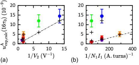
Figure 3: Noise analysis. (a) and (b): Experimental uncertainties, $u^{\mathrm{A}}_{\mathrm{exp}}$, determined from all data for a normalized measurement time ($\tau=16\tau_{0}\sim$ 18 min) and the I_± measurement protocol, as a function of $1/V_{2}$ (a) and $1/N_{1}I_{1}$ (b): $\tiny{\color[rgb]{.54,.17,.888}\hexagofill}$ ($57.42~{}\mu$A, $N_{1}=160$), $\tiny{\color[rgb]{1,0,0}\circletfill}$ ($45.94~{}\mu$A, $N_{1}=160$), $\tiny{\color[rgb]{1,0,0}\rhombusfill}$ ($45.94~{}\mu$A, $N_{1}=465$), $\tiny{\color[rgb]{1,.5,0}\circletfill}$ ($43.07~{}\mu$A, $N_{1}=160$, $n_{1}=1920$), $\tiny{\color[rgb]{0,1,0}\circletfill}$ ($11.48~{}\mu$A, $N_{1}=465$), $\tiny{\color[rgb]{0,0,1}\circletfill}$ ($5.74~{}\mu$A, $N_{1}=160$). Calculated uncertainties, $u^{\mathrm{A}}_{\mathrm{calc}}$ ($\linevh$). Functions 8.8$\times 10^{-10}/V_{2}$ (dash-dotted line in (a)) and $1.6\times 10^{-11}/(N_{1}I_{1})$ (dash-line in (b)) represent $u^{\mathrm{A}}_{\mathrm{calc}}(\tau_{m})$ calculated for $S_{\Phi}=0$ and $S_{V}=0$, respectively.

Evaluation of short-term noise sources
The analysis of the $u^{\mathrm{A}}$ uncertainties provide a further insight into the understanding of the experiment. Fig.3a and b show averages, $u^{\mathrm{A}}_{\mathrm{exp}}(\tau_{m})$, of the $u^{\mathrm{A}}$ uncertainties measured in the different accuracy tests, after normalization to the same measurement time $\tau_{m}=16\tau_{0}$ (with $\tau_{0}=66$ s, $\tau_{m}\sim$ 18 min) and to the same measurement protocol I_±, as a function of $1/V_{2}$ and $1/N_{1}I_{1}$ respectively. For comparison, they also report the theoretical standard uncertainties, $u^{\mathrm{A}}_{\mathrm{calc}}(\tau_{m})=\frac{\sqrt{3}}{16}\sqrt{\frac{S_{\Delta I/I}}{\tau_{A}}}$, calculated using $\tau_{A}=12$ s from the $\Delta I/I$ noise density (Methods) :

$$\sqrt{S_{\Delta I/I}}=\sqrt{\frac{S_{V}}{V_{2}^{2}}+(\frac{1}{N_{1}I_{1}}\gamma_{\mathrm{CCC}})^{2}S_{\phi}},$$ (5)

using a voltage noise of $\sqrt{S_{V}}=\mathrm{28~{}nV/Hz^{1/2}}$ and a magnetic flux noise detected by the SQUID of $\sqrt{S_{\phi}}=6.2\times 10^{-5}\phi_{0}/\mathrm{Hz}^{1/2}$, compatible with the experimental conditions (Extended Data fig.2). Note that there is a satisfying agreement. Fig.3a confirms that, at low $V_{2}$, the main noise contribution comes from the voltage noise of the quantum voltmeter, as emphasized by the $1/V_{2}$ dependence which is reproduced by $u^{\mathrm{A}}_{\mathrm{calc}}(\tau_{m})$ calculated for $S_{\phi}=0$. On the other hand, at higher $V_{2}$ (fig.3b), the number of ampere$\cdot$turns becomes the dominant parameter and the experimental uncertainties follow the $1/N_{1}I_{1}$ dependence of $u^{\mathrm{A}}_{\mathrm{calc}}(\tau_{m})$ calculated for $S_{V}=0$. One can therefore deduce the Type A uncertainty contributions of the PQCG and the quantum voltmeter, which amount to $1.6\times 10^{-11}/(N_{1}I_{1})$ and 8.8$\times 10^{-10}/V_{2}$, respectively. The low value of $7.3\times 10^{-10}$ calculated for $N_{1}=465$ and $I_{1}=45.94~{}\mu$A for the PQCG itself allows considering the generation of even smaller currents. However, the demonstration of their accuracy would require the increase of $R_{2}$, by using a series quantum Hall array of 1.29 $\mathrm{M\Omega}$ resistance Poirier et al. (2004) to increase $V_{2}$.

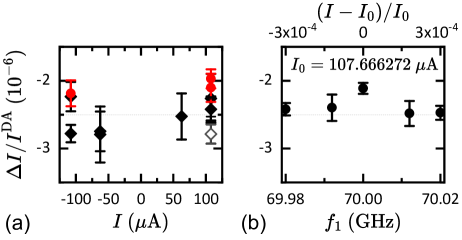
Figure 4: Calibration of a digital ammeter HP3458A. (a) Relative deviation, $\Delta I/I^{\mathrm{DA}}$, as a function of current value in 100 $\mu$A range for different PQCG configurations: $N_{1}=465$, $N_{2}=93,160$ ($\tiny{\color[rgb]{0,0,0}\rhombusfill}$), double connection with $N_{1}=465$, $N_{2}=93$ and application the correction $\alpha_{2}$ ($\tiny{\color[rgb]{0,0,0}\rhombus}$), $N_{1}=160$, $N_{2}=32$ ($\tiny{\color[rgb]{1,0,0}\circletfill}$). Calibrations performed at $\pm$107.7 $\mu$A using either $N_{1}$=465 or $N_{1}$=160, or using the double connection scheme and applying the cable correction $\alpha_{2}$ are all in agreement. (b) $\Delta I/I^{\mathrm{DA}}$ as a function of the Josephson frequency $f_{1}$, or relative deviation of current around $I_{0}=107.666272$ $\mu$A ($\tiny{\color[rgb]{0,0,0}\circletfill}$).

Application to an ammeter calibration
Fig.4a shows the relative deviations $\Delta I/I^{\mathrm{DA}}$ between the currents measured by the DA and the quantized currents generated by the PQCG in the 100 $\mu$A range using the configuration of $\mathrm{PJVS_{1}}$ with $n_{1}=1920$ (Extended Data Table 3). The coarse adjustment of the quantized current, about $\pm$107.7$~{}\mu$A and $\pm$62.6$~{}\mu$A, is done by using $G=465/93$ (or 160/32) and $G=465/160$ respectively. Allan deviation (Extended Data fig.6b) shows that the Type A relative uncertainty for the $\tau_{m}=144$ s measurement time amounts to about $2\times 10^{-7}$ at $\pm$107.7$~{}\mu$A using either I₊ or I_- measurement protocols (Extended Data fig.6a). Data demonstrate that the DA is reproducible over the current range within about 5 parts in $10^{7}$, similar to results obtained in the mA range Brun-Picard et al. (2016). Finally, fig.4b illustrates the possibility of a fine tuning of the current by varying $f_{\mathrm{J}}$ from 69.98 to 70.02 GHz, which represents a relative shift of the quantized current of $\pm 3\times 10^{-4}$ around $107.7$ $\mu$A.

The quantum current standard: state-of-the-art and perspectives
We have demonstrated the accuracy of the flow rate of electrons generated by the new generation PQCG, at current values bridging the gap between the $\mu$A range and the mA range with relative uncertainties $\leq 10^{-8}$, as summarized in inset of fig.5. Moreover, Type A uncertainties of only a few $10^{-9}$ have been measured. These progress stem from eliminating the need of any classical correction, improving the signal-to-noise ratio, extending the operating margins and applying new measurement protocols based on tuning Josephson frequencies. These results open the way to a quantum current standard as accurate as voltage and resistance standards in the future.

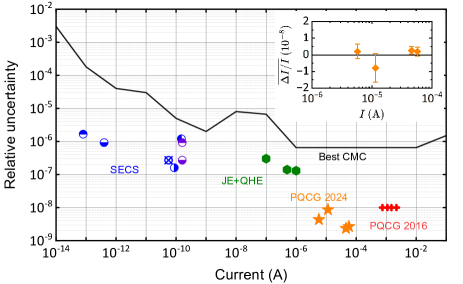
Figure 5: State-of-the-art of the accuracy of quantum current sources and current generation. Comparison between the relative uncertainty achieved in the generation of currents traceable to the ampere using the PQCG ($\tiny{\color[rgb]{1,.5,0}\starletfill}$-this work,$\tiny{\color[rgb]{1,0,0}\linevh}$-Brun-Picard et al. (2016)) and others quantum current sources: metallic ($\tiny{\color[rgb]{0,0,1}\circletfillha}$-Camarota et al. (2012),$\tiny{\color[rgb]{0,0,1}\circletfillhb}$-Keller et al. (2007)), GaAs ($\tiny{\color[rgb]{0,0,1}\circletfillhl}$-Giblin et al. (2012),$\tiny{\color[rgb]{0,0,1}\circletfillhr}$-Stein et al. (2017),$\tiny{\color[rgb]{0,0,1}\circletcross}$-Bae et al. (2020)) and Si ($\tiny{\color[rgb]{.54,.17,.888}\circletfillha}$-Yamahata et al. (2016),$\tiny{\color[rgb]{.54,.17,.888}\circletfillhb}$-Zhao et al. (2017)) SECS, series connection of QHRS array and PJVS for generating ($\tiny{\color[rgb]{.132,.545,.132}\hexagofill}$-Chae et al. (2022)) current. CMCs (black line)BIP (2024). Inset: $\overline{\Delta I/I}$ measurements performed in this work ($\tiny{\color[rgb]{1,.5,0}\rhombusfill}$) as a function of current value $I$. The value at 45.94 $\mu$A corresponds to the weighted mean of $\overline{\Delta I/I}$ values obtained using $N_{1}=160$ and $N_{1}=465$.

Fig.5 shows the state-of-the-art of the accuracy tests of quantum current sources based on different quantum technologies, along with the best calibration measurement capabilities (CMCs) achieved in national metrology institutes (NMIs) for comparison. It recalls the uncertainties achieved in the present work along with those reported in our previous work Brun-Picard et al. (2016). This illustrates the wide range of current covered by the quantum current standard. At much lower currents, around 100 pA, uncertainties at the level of $10^{-7}$ are achieved by the best SECS. This uncertainty level is also reached for currents around 1 $\mu$A by one experiment based on the series connection of quantum Hall resistance array and PJVS Chae et al. (2022). Let us remark that the uncertainties achieved depend not only on the current source itself but also on the method used to measure the generated current. To this respect, the best known measurement techniques reach relative uncertainties of about $10^{-7}$: Giblin (2019)Scherer et al. (2019) (from 100 pA to 1 $\mu$A), Chae et al. (2020) (around 1 $\mu$A), Lee et al. (2016) (around 10 mA). On the other hand, the uncertainties $<10^{-8}$ demonstrated with the PQCG comes not only from its own accuracy and stability but also from the measurement with the quantum voltmeter. Providing such an accurate primary quantum current standard in the current range of the best CMCs, which are limited by uncertainties two orders of magnitude larger, is essential both to improve the transfer of the ampere towards end-users and to foster the development of more accurate instruments, as emphasized by the calibration of a digital ammeter with uncertainties limited by the instrument itself.

Fig.5 also emphasizes the importance of exploring PQCG capabilities towards even smaller currents, in order to bridge the gap in the current delivered by SECS and devices exhibiting dual Shapiro steps. This would open the way to a new metrological triangle experiment Likharev and Zorin (1985); Pekola et al. (2013). More precisely, considering the variant of the PQCG proposed in Poirier et al. (2014) and the noise level estimated in this work, we could expect generating and measuring a 10 nA current with a relative uncertainty of $5\times 10^{-8}$ after 12 h measurement ($N_{1}=160$, $I_{1}=0.33~{}\mu$A, $N_{2}=5400$). Another important result is the demonstration of the PQCG accuracy using a 129 times larger resistance (QHRS₂) than in Brun-Picard et al. (2016), which shows its robustness against the load resistance, as required for a true current source. Moreover, the PQCG accuracy being now established, our experiments can be interpreted as calibrations of resistors of 13 k$\Omega$ and 100 $\Omega$ values with a $10^{-8}$ measurement uncertainty. More generally, combining equations (1) and (2) leads to :

$$R_{\mathrm{2}}=\frac{h}{2e^{2}}\frac{N_{\mathrm{2}}}{N_{\mathrm{1}}}\frac{n_{\mathrm{2}}}{n_{\mathrm{1}}}\frac{f_{\mathrm{2}}^{eq}}{f_{\mathrm{1}}},$$ (6)

where the equilibrium can be coarsely set by choosing $G$ and $n_{1,2}$ and finely tuned by adjusting $f_{1}$ and $f_{2}^{eq}$. This new method combining the PQCG and the quantum voltmeter (see Extended Data fig.3) paves the way for a paradigm shift for the resistance calibration. It allows to simplify the calibration of a large resistance from $\frac{h}{2e^{2}}$ to a single step, suppressing the intermediate steps needed using a conventional resistance comparison bridgePoirier et al. (2021). Furthermore, the full quantum instrumentation developed gives foundation to a DC quantum calibrator-multimeter able to provide the primary references of voltage, resistance and current, which are needed in NMIs. In this perspective, graphene-based single Hall bar Lafont et al. (2015); Ribeiro-Palau et al. (2015) or arrays Panna et al. (2021); He et al. (2023) replacing GaAs devices could provide both noise reduction and simplification of the instrument operation. In the longer term, QHRS based on the quantum anomalous Hall effect Fox et al. (2018); Götz et al. (2018); Okazaki et al. (2022), operating at zero magnetic field as PJVS, or even heterostructures-based JJ comprising stacked cuprates Martini et al. (2024) could lead to a more compact and practical instrumentation.

Acknowledgments This work was supported by the French National Metrology Network (RNMF) (”The ampere metrology” project, number 168). We wish to acknowledge Mohammed Mghalfi for its technical support. We thank D. Estève, D.C. Glattli (CEA/SPEC, France), Yannick De Wilde (ESPCI, France) and Almazbek Imanaliev (LNE, France) for their critical reading and comments.

Author contributions S. D. and W. P. planned the experiments. R. B performed the cabling and the characterizations of the programmable Josephson standards fabricated by PTB. S. D. and W. P. developed the instrumentation, conducted the electrical metrological measurements, analyzed the data and wrote the paper. All authors contributed to the final version.

Competiting interests The authors declare no competiting interest.

I Methods

Quantum devices
Implementation. The two quantum Hall resistance standards, $\mathrm{QHRS_{1}}$ and $\mathrm{QHRS_{2}}$, are both cooled down in the same cryostat at 1.3 K under of magnetic field of 10.8 T. $\mathrm{PJVS_{1}}$ is cooled down in a small amount of liquid helium maintained at 4.2 K in a recondensing cryostat based on a pulse-tube refrigerator while $\mathrm{PJVS_{2}}$ is cooled down in a 100 l liquid He Dewar at 4.2 K. The quantization state of PJVS and QHRS is periodically checked following technical guidelines Rüfenacht et al. (2018)Delahaye and Jeckelmann (2003). In case of occasional trapped flux in the PJVS, a quick heating of the array allows to fully restore the quantized voltage steps. Finally, the CCC is placed in another liquid He Dewar. Connecting five quantum devices, while ensuring quantized operation of PJVS devices and minimizing noise, is very challenging. Many efforts have been spent in optimizing the wiring, the positions of the grounding points and the bias configuration of the PJVS.
Shielding. It is essential to cancel the leakage current that could alter the accurate equality of the total currents circulating through the QHRS and the windings. This is achieved by placing high- and low-potential cables (high-insulation $R_{L}>1$ T$\Omega$ resistance) connected to the PJVS, to the QHRS and to the CCC inside two separated shields, which are then twisted together and connected to ground. In this way, direct leakage currents short circuiting the QHRS, the most troublesome, are canceled. Other leakage currents are redirected to ground.
PJVS cabling. The two PJVS are binary divided 1 V $\mathrm{Nb/Nb_{x}Si_{1-x}/Nb}$ series arrays Behr et al. (2012), both having a total of 8192 JJ and working around 70 GHz. The sequence of the segments that can be biased in the Josephson arrays is the following : 4096/2048/1024/512/256/128/1/31/32/64. Three bondings wires have been added at both ends of the arrays, on the same superconducting pad, in order to implement the triple connection as illustrated in fig.1. A 50 $\Omega$ heater is placed close to the Josephson array chip allowing to get rid of trapped flux within few minutes. We have used a prototype of the hermetic cryoprobe developed for the recondensing cryostat, which had only 8 available wires, reducing the possible wiring configurations for $\mathrm{PJVS_{1}}$. Extended Data fig.1a and b show the two wiring configurations used with $n_{1}=4096$ and $n_{1}=1920$ respectively. They differ essentially on the way the triple connection is implemented at the low potential side of the bias source (PJBS). In Extended Data fig.1a, the triple connection is done on the same superconducting pad, while in Extended Data fig.1b, JJ are present between the bias wire and the wires connecting $\mathrm{QHRS_{1}}$, but also between the second and third connection of the triple connection. If the current circulating in the JJ is less than half the amplitude of the $n=0$ Shapiro step ($<500$ $\mu$A), both configurations are equivalent. However, the second one turned out to be less reliable than the first one when connecting the rest of the circuit. Because of the ground loop including the JJ, it was very sensitive to trapping magnetic flux. Nonetheless, the results of Extended data fig.5c show that quantized currents can be generated using this configuration. It was used for the calibration of the DA. The best accuracy tests reported in fig.2 and Extended Data fig.5a were done with the first configuration.

CCC for correction free PQCG
Design. The new CCC (Extended Data fig.2a and b) is made of 20 windings of 1, 1, 1, 2, 2, 16, 16, 16, 32, 64, 128, 128, 160, 160, 465, 465, 1600, 1600, 2065 and 2065 turns, with a total number of 8789 turns. They are embedded in a superconducting toroidal shield made of 150 $\mu$m thick Pb foils, forming three electrically isolated turns to prevent non-ideal behaviour at the ends of the shield. The architecture is inspired from the design of a CCC used in a quantum Hall resistance bridge Poirier et al. (2021) (enabling ratios close to 1.29), but with 5 additional windings. The triple connection is possible for the windings of 1, 2, 16, 128, 160, 465 and 1600 turns. The dimensions have been chosen to be mounted on a cryogenic probe designed to be compatible with a 70 mm diameter neck of a liquid He Dewar. The inner and outer diameter of the toroidal shield are 19 mm and 47 mm respectively. The chimney is about 125 mm high. The CCC is enclosed in two successive 0.5 mm thick Pb superconducting cylindrical screens and in a Cryoperm shield surrounding the whole, corresponding to an expected overall magnetic attenuation of about 200 dB. It is equipped with a Quantum Design Inc. DC SQUID, placed in a separate superconducting Nb shield, and coupled to the CCC via a superconducting flux transformer composed of a wire wound sensing coil placed as close as possible to the inner surface of the CCC. The coupling $\gamma_{\mathrm{CCC}}=8$ $\mu$A$\cdot$turn/$\phi_{0}$ has been maximized with a sensing coil of 9 turns compatible with the geometrical constraints. The 20 windings are connected by 40 copper alloy wires (AWG 34) placed in a stainless steel shield.
Noise. Extended Data fig.2c shows the noise spectrum at the output of the SQUID. The base noise level of the CCC (green line) amounts to 10 $\mu\phi_{0}/\sqrt{\mathrm{Hz}}$ at 1 Hz in the best noise conditions, slightly higher than the white noise level of 3 $\mu\phi_{0}/\sqrt{\mathrm{Hz}}$ of the SQUID alone (black line). Below 1 Hz, one can observe an increased noise compatible with a 1/$f$ noise contribution. Resonance peaks present at frequencies below 10 Hz are certainly due to an imperfect decoupling of the Dewar from the ground vibrations Poirier et al. (2021).
Damping circuit. A damped resonance at 1.6 kHz is due to the use of a damping circuit to improve the stability of the feedback loop. The damping circuit is made of a $C_{\mathrm{D}}=100$ nF capacitance at room temperature in series with a $R_{\mathrm{D}}=$ 1 k$\Omega$ resistor and a $N_{\mathrm{D}}=$ 2065 turns CCC winding at $T_{\mathrm{D}}=$ 4.2 K. It strongly damps the CCC resonances (around 10 kHz) which are excited by the external noise captured. The counterpart is an increase of the magnetic flux noise detected by the SQUID around 1.6 kHz caused by the Johnson-Nyquist noise emitted by the resistor. However, placing the resistor at low temperature reduced the noise magnitude by a factor of ten compared to the previous experiment Brun-Picard et al. (2016), with a maximum flux noise of $\frac{N_{\mathrm{D}}}{\gamma_{\mathrm{CCC}}}\sqrt{\frac{4k_{\mathrm{B}}T_{\mathrm{D}}}{R_{\mathrm{D}}}}\simeq$ 124 $\mu\phi_{0}/\sqrt{\mathrm{Hz}}$ at 1.6 kHz Djordjevic et al. (2021). In the experimental conditions of this paper, the noise was measured slightly higher, as described by blue curve in Extended Data fig.2c. The noise level at 1 Hz rises to about 20 $\mathrm{\mu\phi_{0}/Hz^{1/2}}$.
Current sensitivity. It is related to the flux generated by the screening current circulating on the shield and can be estimated from the CCC noise spectrum and $\gamma_{\mathrm{CCC}}$, it corresponds to 80 pA$\cdot$ turns/$\sqrt{\mathrm{Hz}}$ at 1 Hz in the best conditions.
Accuracy. The CCC accuracy can be altered by magnetic flux leakage detected by the pickup coil. It can be tested by series opposition measurements of windings of identical number of turns. In the best noise conditions, with a current of 30 to 100 mA, for $N>16$ turns used in this paper the relative error on the number of turns $\delta N/N$ is $<10^{-9}$.

The quantum voltmeter
The quantum voltmeter is made of a second PJVS, PJVS₂ and of nanovoltmeter (EMN11 from EM electronics). It is used to measure the drop voltage at the terminals of the resistor $R_{2}$. The low potential of PJVS₂ is connected at ground, as described in Extended Data fig.3. Direct current leakage parallel to $R_{2}$ are strongly screened by the shielding: no current can circulate between the low potential of $R_{2}$ and ground, because both are at the same potential at equilibrium. All current leakages to ground are deviated in parallel to PJVS₂.

Multiple series connection
In the multiple series connection (see fig.1 and Extended Data fig.1a), the series resistances of the connections result in an effective resistance, which adds to the quantized Hall resistance Delahaye (1993); Poirier et al. (2014). This leads to a lower value of the quantized current $I_{\mathrm{PQCG}}=Gn_{\mathrm{1}}ef_{\mathrm{1}}(1-\alpha_{n})$, where $\alpha_{n}$ is positive and exponentially decreasing with the number of connections $n$. The series resistances $r_{1}$, $r_{2}$, $r_{3}$, $r^{{}^{\prime}}_{1}$, $r^{{}^{\prime}}_{2}$ and $r^{{}^{\prime}}_{3}$, as indicated in Extended Data fig.1a, one calculates, using a Ricketts and Kemeny model Ricketts and Kemeny (1988) of the Hall bar, $\alpha_{2}=\frac{r_{1}r_{2}}{R_{\mathrm{H}}^{2}}+\frac{r^{{}^{\prime}}_{1}r^{{}^{\prime}}_{2}}{R_{\mathrm{H}}^{2}}$ and $\alpha_{3}=\frac{r_{1}r_{2}r_{3}}{R_{\mathrm{H}}^{3}}+\frac{r^{{}^{\prime}}_{1}r^{{}^{\prime}}_{2}r^{{}^{\prime}}_{3}}{R_{\mathrm{H}}^{3}}$ for the double series connection and the triple series connection respectively. The series resistances to be considered are those of the QHRS contacts and cables, those of the long cables linking the quantum devices, and those of the different combinations of CCC windings necessary to obtain the desired number of turns $N_{1}$. For all the experiments based on the triple connection technique, $\alpha_{3}$ is calculated below $1.5\times 10^{-10}$, except for the measurement performed with a 50 $\Omega$ resistor added in series with the first CCC winding (see fig.2e and Extended Data fig.5b), which results in $\alpha_{3}=(1.44\pm 0.023)\times 10^{-9}$. For the measurement reported in fig.2e and in Extended Data fig.5b using the double connection scheme, one calculates $\alpha_{2}=(2.344\pm 0.037)\times 10^{-7}$.

Experimental settings of the PQCG for generating output currents
All accuracy tests are performed using the PQCG settings reported in Extended Data Table 2, except one measurement at 5.74 $\mu$A using frequencies $f_{1}=f_{2}=70.02$ GHz (see fig.2a) and one measurement at 45.94 $\mu$A which uses different frequencies $f_{1}=70$ GHz and $f_{2}=69.999976$ GHz, respectively to accommodate for the deviation of a few parts in $10^{7}$ of the PQCG current from equation (1) caused by the implementation of the double connection only (see fig.2e). Measurements are carried out with $\Delta f$=40 or 80 kHz.

Uncertainties, weighted mean values, combined results and errors bars
Two types of measurement uncertainties are considered: the Type A uncertainties which are evaluated by statistical methods, the Type B uncertainties evaluated by others methods.

Type A uncertainty. The type A uncertainty for one measurement of $\Delta I/I$, $u^{\mathrm{A}}$, is given by :

$$u^{\mathrm{A}}=\frac{u^{\mathrm{A}}(f_{\mathrm{2}}^{eq})}{f_{\mathrm{1}}}$$ (7)

where

$$u^{\mathrm{A}}(f_{\mathrm{2}}^{eq})=\frac{(f_{\mathrm{2}}^{+}-f_{\mathrm{2}}^{-})\sqrt{(w^{\mathrm{A}}_{+}\overline{\Delta V_{f_{2}^{-}}})^{2}+(w^{\mathrm{A}}_{-}\overline{\Delta V_{f_{2}^{+}}})^{2}}}{(\overline{\Delta V_{f_{2}^{+}}}-\overline{\Delta V_{f_{2}^{-}}})^{2}}$$ (8)

with $w^{\mathrm{A}}_{+}$ and $w^{\mathrm{A}}_{-}$ the standard uncertainties (coverage factor $k=1$) of the mean voltage series $\Delta V_{f_{2}^{+}}$ and $\Delta V_{f_{2}^{-}}$, respectively. Their calculation is legitimated by the time dependence of the Allan deviation which demonstrates a dominant white noise (Extended Data fig.4b).

To account for the intra-day noise observed in measurements reported in fig.2e and g, a Type A uncertainty, $u^{\mathrm{A}}_{\mathrm{id-noise}}=10^{-8}$, is added to each data points. Its value was determined so that the $\chi^{2}=\frac{1}{N}\Sigma_{1}^{N}\frac{(X_{i}-\overline{X})^{2}}{u(X_{i})^{2}}<1$ criterion is fulfilled, where here $N$ is the number of values, $X_{i}$ the value, $\overline{X}$ the weighted mean of all $X_{i}$ and $u(X_{i})$ the standard uncertainty of the $X_{i}$. As suggested by an investigation of the quality of the power line of our laboratory, the observed intra-day noise could be caused by a recent increase of the electrical noise pollution.

Type B uncertainty. Extended Data Table 1 shows the basic Type B standard uncertainty budget of the accuracy test, which includes contributions of both the PQCG and the quantum voltmeter. The implementation of the triple series connection and the use of new measurement protocols based on the adjustment of the current using only the Josephson parameters have cancelled (current divider) or strongly reduced (cable correction) the most important contributions of the previous experiment Brun-Picard et al. (2016). We would expect a total uncertainty below $1\times 10^{-9}$. However, it turns out that we measured, momentarily during the measurement campaign, CCC ratio errors slightly higher than the typical values. The ratio errors ranged from $2\times 10^{-9}$ to $0.1\times 10^{-9}$ for windings of number of turns from 128 to 1600, respectively, which were used either for $N_{1}$ or $N_{2}$ in the experiment reported here. Using a conservative approach, we have therefore considered here a Type B uncertainty of $2\times 10^{-9}$ for the CCC, which dominates the uncertainty budget. Other components were detailed in Brun-Picard et al. (2016). The SQUID electronic feedback is based on the same SQUID type and same pre-amplifier from Quantum Design. It is set in the same way using a $4.2~{}V/\phi_{0}$ close-loop gain whatever the number of turns $N_{2}$ used. The VCCS current source preadjusts the output current, such that the SQUID feedbacks only on a small fraction lower than $2\times 10^{-5}\times I_{\mathrm{PQCG}}$ (see Brun-Picard et al. (2016)). Owing to the cable shields, leakage to ground are redirected to ground, i.e. parallel to CCC winding Poirier et al. (2014). The current leakage error amount to $r_{1}/R_{L}$, which is below $7\times 10^{-12}$ in our experiments. It results a relative Type B uncertainty of $2\times 10^{-9}$ for the PQCG and a relative Type B uncertainty of $u_{\mathrm{B}}=2.1\times 10^{-9}$ for the accuracy test.

Weighted mean values. Weighted mean values, $\Delta I/I_{\mathrm{WM}}$ and their uncertainties, $u^{\mathrm{A}}_{\mathrm{WM}}$, are calculated from the $\Delta I/I$ series values and their Type A uncertainties.
In fig.2b and d, they are given by:

$$\Delta I/I_{\mathrm{WM}} =\frac{\sum_{j}\Delta I/I_{j}\times\frac{1}{(u^{\mathrm{A}}_{j})^{2}}}{\sum_{j}\frac{1}{(u^{\mathrm{A}}_{j})^{2}}}$$ (9)

$$u^{\mathrm{A}}_{\mathrm{WM}} =\frac{1}{\sqrt{\sum_{j}\frac{1}{(u^{\mathrm{A}}_{j})^{2}}}}$$ (10)

In fig.2f and h, they are given by:

$$\Delta I/I_{\mathrm{WM}} =\frac{\sum_{j}\Delta I/I_{j}\times\frac{1}{(u^{\mathrm{A}}_{j})^{2}+(u^{\mathrm{A}}_{\mathrm{id-noise}})^{2}}}{\sum_{j}\frac{1}{(u^{\mathrm{A}}_{j})^{2}+(u^{\mathrm{A}}_{\mathrm{id-noise}})^{2}}}$$ (11)

$$u^{\mathrm{A}}_{\mathrm{WM}} =\frac{1}{\sqrt{\sum_{j}\frac{1}{(u^{\mathrm{A}}_{j})^{2}+(u^{\mathrm{A}}_{\mathrm{id-noise}})^{2}}}}$$ (12)

where $u^{\mathrm{A}}_{\mathrm{id-noise}}=10^{-8}$ is the additional Type A component added to each data point to take account of the intra-day noise.


Combined results $\overline{\Delta I/I}$.
For accuracy tests performed at 11.48 $\mu$A using $N_{1}=465$ and at 45.94 $\mu$A using $N_{1}=465$, the combined result $\overline{\Delta I/I}$ is the mean value of the $\Delta I/I_{\mathrm{WM}}$ values obtained using the measurement protocol I₊ and I_-: $\overline{\Delta I/I}=(\Delta I/I_{\mathrm{WM}}(\mathrm{I}_{+})+\Delta I/I_{\mathrm{WM}}(\mathrm{I}_{-}))/2$.
For accuracy tests performed at 5.74 $\mu$A using $N_{1}=160$, at 45.94 $\mu$A using $N_{1}=160$, at 57.42 $\mu$A using $N_{1}=160$ and at 43.07 using $n_{1}=1920$, the combined result $\overline{\Delta I/I}$ is the weighted mean value calculated from the values $(\Delta I/I_{\mathrm{WM}}(\mathrm{I}_{+})+\Delta I/I_{\mathrm{WM}}(\mathrm{I}_{-}))/2$ and $\Delta I/I_{\mathrm{WM}}(\mathrm{I}_{\pm})$ and their respective Type A uncertainties.

Combined uncertainties. The combined uncertainty, $u^{\mathrm{c}}_{\mathrm{WM}}$, is given by $u^{\mathrm{c}}_{\mathrm{WM}}=\sqrt{(u^{\mathrm{A}}_{\mathrm{WM}})^{2}+(u^{\mathrm{B}})^{2}}$. The combined uncertainty of $\overline{\Delta I/I}$ is given by $u^{\mathrm{c}}=\sqrt{(u^{\mathrm{A}}_{\overline{\Delta I/I}})^{2}+(u^{\mathrm{B}})^{2}}$

Error bars. Error bars in the different figures represent measurement uncertainties corresponding to one standard deviation (i.e. $k=1$). This means an interval of confidence of 68% if a gaussian distribution law is assumed. These measurement uncertainties are either Type A uncertainties or combined uncertainties.
Figure 2
In a, c, e and g, error bars correspond to only Type A uncertainties, $u^{\mathrm{A}}$.
In b, d, f and g, errors bars correspond to combined uncertainties, $u^{\mathrm{c}}_{\mathrm{WM}}$
Figure 3
In a and b, errors bars correspond to uncertainties $u(u^{\mathrm{A}}_{\mathrm{exp}})$, which are standard deviations of $u^{\mathrm{A}}$ values, and not standard deviations of the means, in order to reflect the ranges over which the noise levels vary.
Figure 4
In a and b, error bars correspond to Type A standard uncertainties.
Figure 5
In inset of fig.5a, error bars correspond to combined standard uncertainties, $u^{\mathrm{c}}$.
Extended Data figure 5
In a, error bars correspond to combined standard uncertainties $\sqrt{(u^{\mathrm{A}})^{2}+(u^{\mathrm{B}})^{2}}$.
In b, error bars correspond to the combination of Type A standard uncertainties according to $\sqrt{(u^{\mathrm{A}})^{2}+u^{\mathrm{A}}(\Delta I_{\mathrm{ref}}/I_{\mathrm{ref}})^{2}}$.
In c, error bars correspond to $u^{\mathrm{A}}$.

Experimental, $u^{\mathrm{A}}_{\mathrm{exp}}$ and calculated, $u^{\mathrm{A}}_{\mathrm{calc}}$, standard uncertainties.
The uncertainties $u^{\mathrm{A}}_{\mathrm{exp}}(\tau_{m})$ are calculated by averaging the uncertainty values, $u^{\mathrm{A}}$, of each series, after normalization to the same measurement time $\tau_{m}=N_{s}\tau_{0}$ where $N_{s}=16$ is the number of sequences, and to the same measurement protocol I_±. The standard deviation, $u(u^{\mathrm{A}}_{\mathrm{exp}})$, is calculated from the different values of a series. $u^{\mathrm{A}}_{\mathrm{calc}}(\tau_{m})$ is calculated using the relationship $u^{\mathrm{A}}_{\mathrm{calc}}(\tau_{m}=N_{s}\tau_{0})=\frac{1}{\sqrt{N_{s}}}\sqrt{\frac{3}{8}}\sqrt{\frac{S_{\Delta I/I}}{2\tau_{A}}}$, where $\tau_{A}=12$ s is the acquisition time for one single voltage measurement (see Extended Data fig.4a) and $\sqrt{S_{\Delta I/I}}$ is the noise density of $\Delta I/I$. More precisely, $\sqrt{\frac{S_{\Delta I/I}}{2\tau_{A}}}$ is the relative standard deviation corresponding to the acquisition time $\tau_{A}$ assuming an effective white noise density. The pre-factor $\sqrt{\frac{3}{8}}$ comes from the combination of the standard deviations corresponding to the measurement protocol I_±, where the voltage of each sequence is obtained by $[(\Delta V(+I)_{1}+\Delta V(+I)_{3})/2-\Delta V(-I)_{2}]$, with $\Delta V(+I)_{1}$, $\Delta V(-I)_{2}$ and $\Delta V(+I)_{3}$ three successive voltage acquisitions, performed with positive current, then negative current, and then positive current (see Extended Data fig.4a). Finally, the factor $\frac{1}{\sqrt{N_{s}}}$ comes from the white noise hypothesis justified by Extended Data fig.4b. The noise density $\sqrt{S_{\Delta I/I}}$ is given by:

$$\sqrt{S_{\Delta I/I}}=\sqrt{\frac{S_{V}}{V_{2}^{2}}+(\frac{1}{N_{1}I_{1}}\gamma_{\mathrm{CCC}})^{2}S_{\phi}+\frac{4kT}{R_{1}I_{1}^{2}}},$$ (13)

where $k$ is the Boltzmann constant and $T$=1.3 K. Three noise contributions are considered: the voltage noise power spectral density, $S_{V}$, of the quantum voltmeter, which includes the noise of the null detector and some external voltage noise captured, the magnetic flux noise power spectral density, $S_{\phi}$, detected by the SQUID, which includes the SQUID noise and some external magnetic flux noise captured and the Johnson-Nyquist noise power spectral density emitted by the resistor $R_{1}$ in the primary loop. The Johnson-Nyquist noise of the resistor $R_{2}$ is included in $S_{V}$. The third term contributes to $\sqrt{S_{\Delta I/I}}$ by about $1.6\times 10^{-9}/\mathrm{Hz}^{1/2}$ for $I_{1}=45.94$ $\mu$A, leading to a negligible uncertainty contribution of $5\times 10^{-11}$ for a measurement time $\tau_{m}=16\tau_{0}$. This third term is therefore not considered in our calculations. Values reported in fig.2e and f are calculated using a voltage noise of $\sqrt{S_{V}}=\mathrm{28~{}nV/Hz^{1/2}}$ and a magnetic flux noise detected by the SQUID of $\sqrt{S_{\phi}}=6.2\times 10^{-5}\phi_{0}/\mathrm{Hz}^{1/2}$.

Measurement protocol for the ammeter calibration
Calibrations of the ammeter HP3458A are performed using settings of the PQCG reported in Extended Data Table 3. In these experiments, output current values are changed by varying both the gain $G$ and the frequency $f_{1}$. Using the PQCG to perform ammeter calibration consists in replacing $\mathrm{QHRS_{2}}$ by the device under test and removing the quantum voltmeter. The connection is done through a low-pass filter (highly insulated PTFE 100 nF on the differential input). A common mode torus has also been introduced to minimize the noise. Extended Data fig.6a shows recordings by the ammeter (HP3458A) as a function of time for several alternations of $I_{\mathrm{PQCG}}$ at 107.666272 $\mu$A using the measurement protocol I₊. The acquisition time, the waiting time are of 10 s and 2 s, respectively. The measured current is determined from the average of the values obtained for several measurement groups. The time dependence of the Allan deviation, reported in Extended Data fig.6b, shows that the standard deviation of the mean is a relevant estimate of the Type-A relative uncertainty at $\tau_{m}=144$ s. An uncertainty of $2\times 10^{-7}$ is typically achieved after a total measurement time of 144 s.

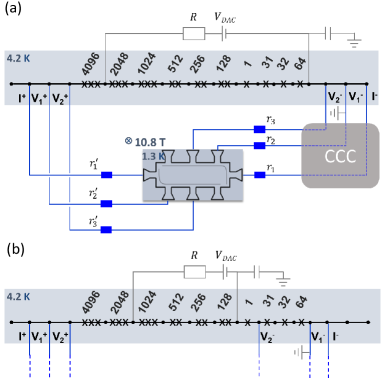
Extended Data Fig. 1: Two wiring configurations for PJVS₁. The PJBS is represented by a voltage source $V_{\mathrm{DAC}}$ and a resistance $R=1$ k$\Omega$. The PJBS is connected to ground at the low potential side with of a capacitance $C=1$ $\mu$F. Black lines : superconducting wires, grey lines : bias lines and connection to ground, blue lines : triple connection. (a) Configuration with $n_{1}=4096$. (b) Configuration with $n_{1}=1920$ (CCC and QHRS₁ are not represented).

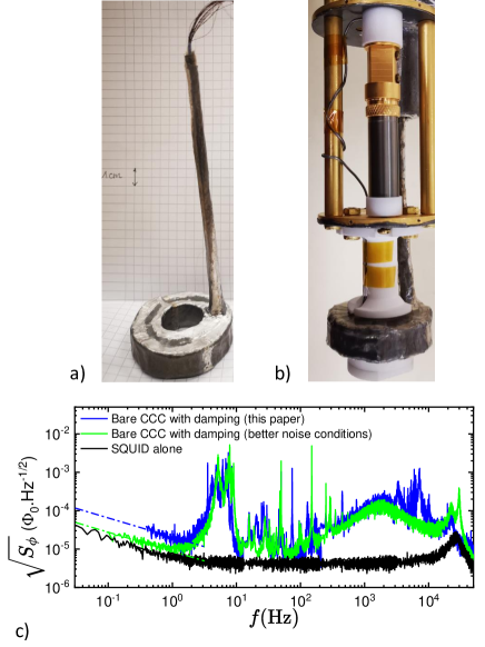
Extended Data Fig. 2: CCC details. (a) Photo of the CCC. (b) Photo of the CCC mounted in the cryogenic probe. (c) Flux noise measured at the output of the SQUID alone (black line) and coupled to the bare CCC with damping circuit in this work (blue line) and in best conditions (green line). Blue and green dash dotted lines present $1/\sqrt{f}$ slopes.

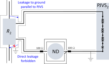
Extended Data Fig. 3: Quantum voltmeter. Scheme of the quantum voltmeter measuring the voltage drop at the terminal of a resistor of resistance $R_{2}$. Thin lines represent the outer shielding of the cables, which is connected to ground. The low potential of PJVS₂ is also connected to ground. At equilibrium, direct current leakage is cancelled. Current leakage to ground is parallel to PJVS₂. One 100 $\Omega$ resistance is added in series on each side of the ND to limit the circulation of strong current during current reversal.

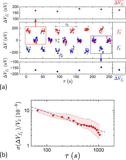
Extended Data Fig. 4: Measurement protocol. (a) ND readings, $\Delta V$, as a function of time, $\tau$, obtained using the measurement protocol I₊ at $11.48440211$ $\mu$A, during the two steps carried out at $f_{2}^{+}$ ($\tiny{\color[rgb]{1,0,0}\circletfill}$) and $f_{2}^{-}$ ($\tiny{\color[rgb]{0,0,1}\circletfill}$), respectively. Here, $f_{1}=f_{2}=70$ GHz and $\Delta f=80$ kHz. At each alternation of $I_{\mathrm{PQCG}}$, a waiting time $\tau_{W}$ of 10 s is applied, and the acquisition time in each state is $\tau_{A}$=12 s. The period time is $\tau_{0}=66$ s. Mean values, $\overline{\Delta V_{f_{2}^{+}}}$ and $\overline{\Delta V_{f_{2}^{+}}}$ are then obtained by averaging the series of voltage values $\Delta V_{f_{2}^{-}}$ and $\Delta V_{f_{2}^{+}}$. Each of these voltage values is itself given by $[(\Delta V(+I)_{1}+\Delta V(+I)_{3})/2-\Delta V(0)_{2}]$, where $\Delta V(+I)_{1}$, $\Delta V(0)_{2}$ and $\Delta V(+I)_{3}$ are three successive voltage measurements performed with positive current switched on, then off, and then on (rectangle). (b) Relative Allan deviation ($\tiny{\color[rgb]{1,0,0}\circletfill}$) calculated from a series of 32 values of $\Delta V_{f_{2}^{+}}$ plotted as a function of $\tau$. The red area corresponds to the 68.3 % confidence interval. The good agreement of the $9\times 10^{-7}\times\tau^{-1/2}$ fit (black dashed line) with data confirms the dominant contribution of the white noise. This legitimate the calculation of standard deviation of the mean to estimate the uncertainties.

Contribution	$\bm{u^{\mathrm{B}}}$
	$\bm{(10^{-9})}$
Triple series connection	0.2
Electronic feedback	$<0.5$
CCC accuracy	$<2$
QHRS1	$<0.1$
PJVS1	$<0.1$
Current leakage	$<0.01$
Frequency	$<0.01$
PQCG	2
QHRS2	$<0.1$
PJVS2	$<0.1$
Null detector	$<0.5$
Quantum voltmeter	0.5
Accuracy test	2.1

Extended Data Table. 1: Basic relative Type B standard uncertainty budget (coverage factor $k=1$) of the accuracy test including contributions of the PQCG and of the quantum voltmeter.

Current	$I_{\mathrm{PQCG}}$	$n_{1}$	$f_{1}=f_{2}$	$I_{1}$	$G$=$N_{1}$/$N_{2}$	$n_{2}$	$V_{2}$
value	($\mu$A)		(GHz)	($\mu$A)			(V)
@ 5.74	5.742201056	4096	70	45.94	160/1280	512	0.074
@11.48	11.48440211	4096	70	45.94	465/1860	1024	0.148
@43.07	43.06650792	1920	70	21.53	160/80	3840	0.556
@45.94	45.93760845	4096	70	45.94	160/160	4096	0.593
@45.94	45.93760845	4096	70	45.94	465/465	4096	0.593
@57.42	57.42201056	4096	70	45.94	160/128	5120	0.741

Extended Data Table. 2: Experimental settings of the PQCG for the accuracy tests.

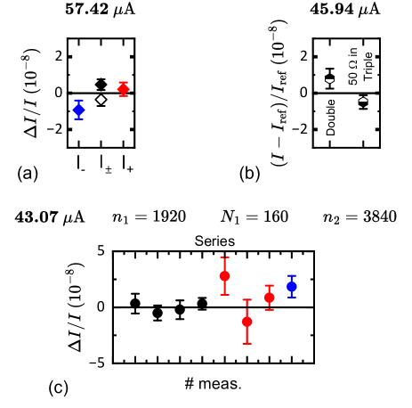
Extended Data Fig. 5: Robustness tests of the PQCG accuracy. (a) Relative deviations $\Delta I/I$ at 57.42201056 $\mu$A measured with $n_{1}=4096$ for I₊ ($\tiny{\color[rgb]{1,0,0}\rhombusfill}$), I_- ($\tiny{\color[rgb]{0,0,1}\rhombusfill}$) and I_± ($\tiny{\color[rgb]{0,0,0}\rhombusfill}$) ($\tiny{\color[rgb]{0,0,0}\rhombus}$: mean value of I₊ and I_-). Errors bars corresponds to combined uncertainties (Methods). (b) Relative current shift from a reference value $I_{\mathrm{ref}}$, in back and forth measurements testing the effectiveness of the triple connection (data extracted from Extended Data fig.2e at 45.94 $\mu$A). Double connection with the $2^{\mathrm{nd}}$ order correction ($\alpha_{2}$) applied ($\tiny{\color[rgb]{0,0,0}\hexagofillha}$). Triple connection with 50 $\Omega$ inserted in the first connection with third order correction $\alpha_{3}$ applied ($\tiny{\color[rgb]{0,0,0}\hexagofillhb}$). The results are consistent within the Type A standard uncertainty. This confirms the accuracy of the cable corrections when applied and the efficiency of the triple connection against large cable resistance value. (c) series of $\Delta I/I$ measurements carried out at 43.06650792 $\mu$A for I_± ($\tiny{\color[rgb]{0,0,0}\circletfill}$), I₊ ($\tiny{\color[rgb]{1,0,0}\circletfill}$) and I_- ($\tiny{\color[rgb]{0,0,1}\circletfill}$)) measurement protocols using a second $\mathrm{PJVS_{1}}$ configuration with $n_{1}=1920$ and $G=N_{1}/N_{2}=160/80$. Errors bars corresponds to $u^{\mathrm{A}}$ uncertainties. Discrepancies are within less than two parts in $10^{8}$. This demonstrates that the PQCG can be accurate within this uncertainty even though the biasing scheme is less robust with respect to trapping magnetic flux (see Extended Data fig.1b).

Current	$I_{\mathrm{PQCG}}$	$n_{1}$	$f_{1}$	$I_{1}$	$G$=$N_{1}$/$N_{2}$
value	($\mu$A)		(GHz)	($\mu$A)
@ 62.58	062.581019	1920	70	21.53	465/160
@107.64	107.635508	1920	69.98	21.53	465/93
@107.65	107.653965	1920	69.992	21.53	465/93
@107.67	107.666270	1920	70	21.53	465/93
@107.68	107.684727	1920	70.012	21.54	465/93
@107.70	107.697032	1920	70.02	21.54	465/93
@107.67	107.666270	1920	70	21.53	160/32

Extended Data Table. 3: Experimental settings of the PQCG for the ammeter calibration

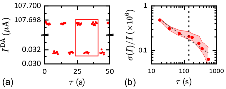
Extended Data Fig. 6: (a) Data recorded by the HP3458A of $I_{\mathrm{PQCG}}=107.666272$ $\mu$A as a function of time, $\tau$, for measurement protocol I₊. (b) Time dependence of the Allan deviation. The vertical dash-line is at $\tau=144$ s.

References

- BIPM (9th edition, 2019) BIPM, The International System of units (SI) (http://www.bipm.org/en/si/, Sèvres, 9th edition, 2019).
- Poirier et al. (2019) W. Poirier, S. Djordjevic, F. Schopfer, and O. Thévenot, “The ampere and the electrical units in the quantum era,” C. R. Physique 20, 92 (2019).
- Pothier et al. (1992) H. Pothier, P. Lafarge, C. Urbina, D. Estève, and M. H. Devoret, “Single-electron pump based on charging effects,” Eur. Phys. Lett. 17, 249 (1992).
- Pekola et al. (2013) J. P. Pekola, O. P. Saira, V. Maisi, A. Kemppinen, M. Mttnen, Y. A. Pashkin, and D. Averin, “Single-electron current sources: Toward a refined definition of the ampere,” Rev. Mod. Phys. 85, 1421–1472 (2013).
- Scherer and Schumacher (2019) H. J. Scherer and H. W. Schumacher, “Single-electron pumps and quantum current metrology in the revised SI,” Annalen der Physik 531, 1800371 (2019).
- Keller et al. (1999) M. W. Keller, A. L. Eichenberger, J. M. Martinis, and N. M. Zimmermann, “A capacitance standard based on counting electrons,” Science 285, 1706 (1999).
- Pekola et al. (2008) J. P. Pekola, J. J. Vartiainen, M. Mottonen, O. P. Saira, M. Meschke, and D. V. Averin, “Hybrid single-electron transistor as a source of quantized electric current,” Nature Phys. 4, 120 (2008).
- Camarota et al. (2012) B. Camarota, H. Scherer, M. W. Keller, S. V. Lotkov, G. Willenberg, and J. Ahlers, “Electron counting capacitance standard with an improved five-junction R-pump,” Metrologia 49, 8–14 (2012).
- Giblin et al. (2012) S. P. Giblin, M. Kataoka, J. D. Fletcher, P. See, T. J. B. M. Janssen, J. P. Griffiths, G. A. C. Jones, I. Farrer, and D. A. Ritchie, “Towards a quantum representation of the ampere using single electron pumps,” Nat. Commun. 3, 930 (2012).
- Stein et al. (2015) F. Stein, D. Drung, L. Fricke, H. Scherer, F. Hohls, C. Leicht, M. Götz, C. Krause, R. Behr, E. Pesel, K. Pierz, U. Siegner, F. J. Ahlers, and H. W. Schumacher, “Validation of a quantized-current source with 0.2 ppm uncertainty,” Appl. Phys. Lett. 107, 103501 (2015).
- Stein et al. (2017) F. Stein, H. Scherer, T. Gerster, R. Behr, M. Götz, E. Pesel, C. Leicht, N. Ubbelohde, T. Weimann, K. Pierz, H. W. Schumacher, and F. Hohls, “Robustness of single-electron pumps at sub-ppm current accuracy level,” Metrologia 54, S1 (2017).
- Yamahata et al. (2016) G. Yamahata, S. P. Giblin, M. Kataoka, T. Karasawa, and A. Fujiwara, “Gigahertz single-electron pumping in silicon with an accuracy better than 9.2 parts in ,” Appl. Phys. Lett. 109, 013101 (2016).
- Zhao et al. (2017) R. Zhao, A. Rossi, S. P. Giblin, J. D. Fletcher, F. E. Hudson, M. Möttönen, M. Kataoka, and A. S. Dzurak, “Thermal-error regime in high-accuracy gigahertz single-electron pumping,” Phys. Rev. Appl. 8, 044021 (2017).
- Bae et al. (2020) M.-H. Bae, D.-H. Chae, M.-S. Kim, B.-K. Kim, S.-I. Park, J. Song, T. Oe, N.-H. Kaneko, N. Kim, and W.-S. Kim, “Precision measurement of single-electron current with quantized hall array resistance and josephson voltage,” Metrologia 57, 065025 (2020).
- Kataoka et al. (2011) M. Kataoka, J. D. Fletcher, P. See, S. P. Giblin, T. J. B. M. Janssen, J. P. Griffiths, G. A. C. Jones, I. Farrer, and D. A. Ritchie, “Tunable nonadiabatic excitation in a single-electron quantum dot,” Phys. Rev. Lett. 106, 126801 (2011).
- Ahn et al. (2017) Y.-H. Ahn, C. Hong, Y.-S. Ghee, Y. Chung, Y.-P. Hong, M.-H. Bae, and N. Kim, “Upper frequency limit depending on potential shape in a QD-based single electron pump,” Journal of Applied Physics 122, 194502 (2017).
- Shaikhaidarov et al. (2022) R.-S. Shaikhaidarov, K. H. Kim, J. W. Dunstan, I. V. Antonov, S. Linzen, M. Ziegler, D. S. Golubev, V. N. Antonov, E. V. Ilíchev, and O. V. Astafiev, “Quantized current steps due to the a.c. coherent quantum phase-slip effect,” Nature 608, 45 (2022).
- Crescini et al. (2023) N. Crescini, S. Cailleaux, W. Guichard, C. Naud, O. Buisson, K. W. Murch, and N. Roch, “Evidence of dual shapiro steps in a josephson junction array,” Nat. Phys. 19, 851 (2023).
- (19) V. Gaydamachenko L. Grünhaupt F. Kaap, C. Kissling and S. Lotkhov, “Demonstration of dual Shapiro steps in small Josephson junctions,” arXiv:2401.06599 .
- Kurilovich et al. (2024) V. D. Kurilovich, B. Remez, and L. I. Glazman, “Quantum theory of bloch oscillations in a resistively shunted transmon,” Arxiv:2403.04624v1 (2024).
- Josephson (1962) B.D. Josephson, “Possible new effects in superconductive tunnelling,” Phys. Lett. 1, 251–253 (1962).
- von Klitzing et al. (1980) K. von Klitzing, G. Dorda, and M. Pepper, “New method for high-accuracy determination of the fine structure constant based on quantized Hall resistance,” Phys. Rev. Lett. 45, 494–497 (1980).
- Shapiro (1963) S. Shapiro, “Josephson currents in superconducting tunneling: the effect of microwaves and another observations,” Phys. Rev. Lett. 11, 80–82 (1963).
- Chae et al. (2022) D.-H. Chae, M.-S. Kim, T. Oe, and N.-H. Kaneko, “Series connection of quantum hall resistance array and programmable josephson voltage standard for current generation at one microampere,” Metrologia 59, 065011 (2022).
- Kaneko et al. (2024) N.-H. Kaneko, T. Tanaka, and Y. Okazaki, “Perspectives of the generation and measurement of small electric currents,” Meas. Sci. Technol. 35, 011001 (2024).
- Poirier et al. (2014) W. Poirier, F. Lafont, S. Djordjevic, F. Schopfer, and L. Devoille, “A programmable quantum current standard from the josephson and the quantum hall effects,” J. Appl. Phys. 115, 044509 (2014).
- Brun-Picard et al. (2016) J. Brun-Picard, S. Djordjevic, D. Leprat, F. Schopfer, and W. Poirier, “Practical quantum realization of the ampere from the elementary charge,” Phys. Rev. X 6, 041051 (2016).
- Djordjevic et al. (2021) Sophie Djordjevic, Ralf Behr, Dietmar Drung, Martin Götz, and Wilfrid Poirier, “Improvements of the programmable quantum current generator for better traceability of electrical current measurements,” Metrologia 58, 045005 (2021).
- Behr et al. (2012) R. Behr, O. Kieler, J. Kohlmann, F. Müller, and L. Palafox, “Development and metrological applications of josephson arrays at ptb,” Meas. Sci. Technol. 23, 124002 (2012).
- Piquemal et al. (1993) F. Piquemal, G. Genevès, F. Delahaye, J. P. André, J. N. Patillon, and P. Frijlink, “Report on a joint BIPM-EUROMET project for the fabrication of QHE samples by the LEPs,” IEEE Trans. Instrum. Meas. 42, 264 (1993).
- Harvey (1972) I. K. Harvey, “A precise low temperature dc ratio transformer,” Rev. Sci. Instrum. 43, 1626–1629 (1972).
- Delahaye (1993) F. Delahaye, “Series and parallel connection of multiterminal quantum hall-effect devices,” J. Appl. Phys. 73, 7914 (1993).
- Buttiker (1988) M. Buttiker, “Absence of backscattering in the quantum hall effect in multiprobe conductors,” Phys. Rev. B 38, 9375 (1988).
- Poirier et al. (2004) W. Poirier, A. Bounouh, F. Piquemal, and J. P. André, “A new generation of qhars: discussion about the technical criteria for quantization,” Metrologia 41, 285 (2004).
- Keller et al. (2007) M. W. Keller, N. M. Zimmermann, and A. L. Eichenberger, “Uncertainty budget for the nist electron counting capacitance standard, eccs-1,” Metrologia 44, 505 (2007).
- BIP (2024) “The bipm key comparison database (kcdb), calibration and measurement capabilities – cmcs (appendix c), dc current database.” (2024).
- Giblin (2019) S. P. Giblin, “Re-evaluation of uncertainty for calibration of 100 m and 1 g resistors at npl,” Metrologia 56, 015014 (2019).
- Scherer et al. (2019) H. Scherer, D. Drung, C. Krause, M. Götz, and U. Becker, “Electrometer calibration with sub-partper-million uncertainty,” IEEE Trans. Instrum. Meas. 68, 1887 (2019).
- Chae et al. (2020) D.-H. Chae, M.-S. Kim, W.-S. Kim, T. Oe, and N.-H. Kaneko, “Quantum mechanical current-to-voltage conversion with quantum hall resistance array,” Metrologia 57, 025004 (2020).
- Lee et al. (2016) J. Lee, R. Behr, B. Schumacher, L. Palafox, M. Schubert, M. Starkloff, A. C. Böck, and P. M. Fleischmann, “From ac quantum voltmeter to quantum calibrator,” in CPEM 2016 (2016) pp. 1–2.
- Likharev and Zorin (1985) K. K. Likharev and A. B. Zorin, “Theory of the bloch-wave oscillations in small josephson junctions,” J. Low Temp. Phys. 59, 347 (1985).
- Poirier et al. (2021) Wilfrid Poirier, Dominique Leprat, and Félicien Schopfer, “A resistance bridge based on a cryogenic current comparator achieving sub- measurement uncertainties,” IEEE Transactions on Instrumentation and Measurement 70, 1–14 (2021).
- Lafont et al. (2015) F. Lafont, R. Ribeiro-Palau, D. Kazazis, A. Michon, O. Couturaud, C. Consejo, T. Chassagne, M. Zielinski, M. Portail, B. Jouault, F. Schopfer, and W. Poirier, “Quantum hall resistance standards from graphene grown by chemical vapour deposition on silicon carbide,” Nature Communications 6, 6806 (2015).
- Ribeiro-Palau et al. (2015) R. Ribeiro-Palau, F. Lafont, J. Brun-Picard, D. Kazazis, A. Michon, F. Cheynis, O. Couturaud, C. Consejo, B. Jouault, W. Poirier, and F. Schopfer, “Quantum hall resistance standard in graphene devices under relaxed experimental conditions,” Nature Nano. 10, 965–971 (2015).
- Panna et al. (2021) A. R. Panna, IF. Hu, M. Kruskopf, D. K. Patel, D. G. Jarrett, C.-I Liu, S. U. Payagala, D. Saha, A. F. Rigosi, D. B. Newell, C.-T. Liang, and R. E. Elmquist, “Graphene quantum hall effect parallel resistance arrays,” Phys. Rev. B 103, 075408 (2021).
- He et al. (2023) H. He, K. Cedergren, N. Shetty, S. Lara-Avila, S. Kubatkin, T. Bergsten, and G. Eklund, “Accurate graphene quantum hall arrays for the new international system of units,” Nat. Commun. 13, 6933 (2023).
- Fox et al. (2018) E. J. Fox, I. T. Rosen, Y. Yang, G. R. Jones, R. E. Elmquist, X. Kou, L. Pan, K. L. Wang, and D. Goldhaber-Gordon, “Part-per-million quantization and current-induced breakdown of the quantum anomalous hall effect,” Phys. Rev. B 98, 075145 (2018).
- Götz et al. (2018) M. Götz, K. M. Fijalkowski, E. Pesel, M. Hartl, T. Schreyeck, M. Winnerlein, S. Grauer, H. Scherer, K. Brunner, C. Gould, F. J. Ahlers, and L. W. Molenkamp, “Precision measurement of the quantized anomalous hall resistance at zero magnetic field,” Appl. Phys. Lett. 112, 072102 (2018).
- Okazaki et al. (2022) Y. Okazaki, T. Oe, M. Kawamura, R. Yoshimi, S. NaKamura, S. Takada, M. Mogi, K.-S. Takahashi, A. Tsukazaki, M. Kawasaki, Y. Tokura, and N.-H. Kaneko, “Quantum anomalous hall effect with a permanent magnet defines a quantum resistance standard,” Nat. Phys. 18, 25–29 (2022).
- Martini et al. (2024) M. Martini, Y. Lee, T. Confalone, S. Shokri, C. N. Saggau, D. Wolf, G. Gu, K. Watanabe, T. Taniguchi, D. Montemurro, V. M. Vinokur, K. Nielsch, and N. Poccia1, “Twisted cuprate van der waals heterostructures with controlled josephson coupling,” arXiv:2303.16029v3 (2024).
- Rüfenacht et al. (2018) Alain Rüfenacht, Nathan E. Flowers-Jacobs, and Samuel P. Benz, “Impact of the latest generation of josephson voltage standards in ac and dc electric metrology,” Metrologia 55, S152 (2018).
- Delahaye and Jeckelmann (2003) F. Delahaye and B. Jeckelmann, “Revised technical guidelines for reliable dc measurements of the quantized hall resistance,” Metrologia 40, 217 (2003).
- Ricketts and Kemeny (1988) B. W. Ricketts and P. C. Kemeny, “Quantum hall effect devices as circuit elements,” J. Phys. D 21, 483 (1988).