Bridging Wright-Fisher and Moran models

Abstract

The Wright-Fisher model and the Moran model are both widely used in population genetics. They describe the time evolution of the frequency of an allele in a well-mixed population with fixed size. We propose a simple and tractable model which bridges the Wright-Fisher and the Moran descriptions. We assume that a fixed fraction of the population is updated at each discrete time step. In this model, we determine the fixation probability of a mutant in the diffusion approximation, as well as the effective population size. We generalize our model, first by taking into account fluctuating updated fractions or individual lifetimes, and then by incorporating selection on the lifetime as well as on the reproductive fitness.

I Introduction

A major goal of population genetics is to describe how the frequency of an allele in a population changes over time. Different evolutionary forces shape genetic diversity. In the simplest models of well-mixed haploid populations with fixed size, the fate of a mutant is determined by the interplay of natural selection and genetic drift (in the absence of any additional mutation). The first model incorporating these ingredients dates back to the 1930s and is known as the Wright-Fisher model [1, 2]. This widely used model assumes discrete and non-overlapping generations. Each generation is formed from the previous one through binomial sampling. This model can be extended to include for instance multi-allele selection, additional mutations [3] and is a suitable framework for the inference of selection from genetic data [4, 5, 6]. Another traditional model including natural selection and genetic drift is the Moran process. It considers overlapping generations with one individual birth and one individual death occurring at each discrete time step [7]. Extensions of this model include other birth-death processes, structured population on graphs [8, 9, 10, 11]. This framework is widely applied beyond population genetics, including evolutionary game theory [12, 13, 14]. While the Wright-Fisher model and the Moran model share the same key ingredients and behave similarly, their different detailed dynamics lead to slightly different diffusion equations and mutant fixation probabilities.

Several population genetics models that are more general than the Wright-Fisher and Moran model have been developed. They include the Karlin and McGregor model [15, 16] and the Chia and Watterson model [17]. The latter considers a haploid population of fixed size $N$, where each individual reproduces independently, according to a specific distribution of offspring number. Then $r$ parents and $N-r$ offspring constitute the next generation, where $r$ is a random variable conditioned by the offspring population size. While this encompasses Wright-Fisher and Moran models as particular cases, Chia and Watterson [17] indicated that “there did not seem to be any continuity […]” between these two frameworks. Besides, as pointed out by Cannings [18], the Chia and Watterson model is rather complex since it involves the offspring distribution, the fraction of surviving offsprings, and the sampling of the new generation from the parent and the offspring populations. It makes it hardly tractable, and to our knowledge, the mutant fixation probability has not been derived under this model.

Here, we propose a simple and tractable model which bridges the Wright-Fisher model and the Moran model. Specifically, we assume that a fixed fraction of the population is updated at each discrete time step. We show that our model generalizes over both the Wright-Fisher model and the Moran model. Under Kimura’s diffusion approximation, we obtain a simple expression of the fixation probability of a mutant in our model. We further study the rate of approach to the steady state in the neutral case, and determine the variance effective population size and the eigenvalue effective population size. Next, we generalize our model, first by taking into account fluctuations of the fraction that is updated at each discrete time step, and then by considering individuals with fluctuating lifetimes. This allows us to express the fixation probability as a function of the mean life time of individuals. Finally, we further generalize our model by incorporating selection on the lifetime as well as on the reproductive fitness, i.e., both on birth and death processes, assuming that lifetimes are geometrically distributed.

II Model with fixed updated fraction

II.1 Description of the model

Let us consider a population comprising a fixed number $N$ of haploid individuals. Let us assume that there are two types of individuals, corresponding to wild-type and mutant individuals. Let us denote by $1+s$ the relative fitness of the mutant compared to the wild-type. Let us further denote by $i$ the number of mutant individuals, which fully describes the state of the population, and let us introduce

$$x=\frac{i}{N}\,\,\,\,\textrm{and}\,\,\,\,p=\frac{i(1+s)}{i(1+s)+N-i}=\frac{x(1+s)}{1+xs}\,.$$ (1)

At each discrete time step, we update a fraction of the population as follows (see Fig. 1):

• Choose $M$ individuals uniformly at random in the population, without replacement. $M$ satisfies $1\leq M\leq N$ (in this section, we assume that $M$ is fixed throughout the evolution of the population, and in the next sections, we will present generalizations).

• Replace the $M$ chosen individuals with $M$ new ones, sampled from a binomial distribution with parameters $M$ and $p$.

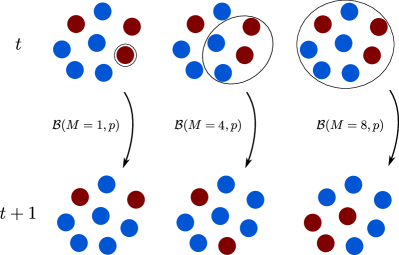
Figure 1: Schematic of three different updates in a population starting from $5$ wild-type individuals (blue) and $3$ mutants (red). Updates are performed by replacing $M$ individuals through binomial sampling with probability $p$ given in Eq. 1. Left: $M=1$ (which corresponds to the Moran model, see Eq. 7), middle: $M=4$, right: $M=N=8$ (Wright-Fisher model).

Link to the Wright-Fisher model.

For $M=N$, we recover the Wright-Fisher model. As a reminder, in the Wright-Fisher model, generations do not overlap. At each discrete step a new generation is sampled from the binomial law with parameters $N$ and $p$, yielding the following transition probabilities for the number of mutants:

$$P_{i\rightarrow j}^{\text{WF}(N)}=\binom{N}{j}{p}^{j}(1-p)^{N-j}\,,$$ (2)

for all $j$ between 0 and $N$.

Formalization of the model.

The number $k$ of mutants among the $M$ individuals sampled from the population follows a hypergeometric distribution with group sizes $i$ and $N-i$ and sample size $M$. Denoting by $q_{N,M,i}(k)$ the probability to draw $k$ mutants according to this distribution, we have:

$$q_{N,M,i}(k)=\frac{\binom{i}{k}\binom{N-i}{M-k}}{\binom{N}{M}}\,.$$ (3)

The transition probabilities for the number of mutants upon each discrete step then read:

$$P_{i\rightarrow j}^{(N,M)}=\sum_{k=0}^{i}q_{N,M,i}(k)P_{i\rightarrow k+j-i}^{\text{WF}(M)}\,,$$ (4)

where $P_{i\rightarrow j}^{\text{WF}(N)}$ is defined in Eq. 2. Note that for $M=N$, we have

$$q_{N,N,i}(k)=\frac{\binom{i}{k}\binom{N-i}{N-k}}{\binom{N}{N}}=\delta_{k,i}\,,$$ (5)

where $\delta_{i,j}$ is 1 if $i=j$ and 0 otherwise, and Eq. 4 reduces to Eq. 2 as expected. Note also that the transition probabilities given in Eq. 4 are duly normalized. Indeed, introducing $m=k+j-i$, we have

$$\sum_{k=0}^{i}q_{N,M,i}(k)\sum_{m=0}^{M}P_{i\rightarrow m}^{\text{WF}(M)}=1\,.$$ (6)

Link to the Moran model.

For $M=1$, Eq. 4 can be simplified into

$$P_{i\rightarrow j}^{(N,1)}=\left\{\begin{array}[]{ll}x(1-p)&\text{if }j=i-1,\\ xp+(1-x)(1-p)&\text{if }j=i,\\ p(1-x)&\text{if }j=i+1,\\ 0&\text{else,}\end{array}\right.$$ (7)

which exactly coincides with the Moran model. Therefore, our model generalizes over both the Wright-Fisher model and the Moran model.

II.2 Mutant fixation probability

Let us consider a large-sized population $N\gg 1$ and assume that $s$ is of order $1/N$. These conditions allow us to employ Kimura’s diffusion approximation [19] (see Supplemental Material (SM) for mathematical details [20]). The fixation probability $\phi(x)$ of the mutant type, starting from a fraction $x$ of mutants in the population, then satisfies the following Kolmogorov backward equation [19]:

$$\frac{\mathbb{V}(\Delta x)}{2}\frac{\mbox{d}^{2}\phi}{\mbox{d}x^{2}}+\mathbb{E}(\Delta x)\frac{\mbox{d}\phi}{\mbox{d}x}=0\,,$$ (8)

where $\Delta x$ is the variation of the mutant fraction occurring in the first discrete time step starting from the initial fraction $x$, and $\mathbb{E}(\Delta x)$ and $\mathbb{V}(\Delta x)$ denote respectively its expected value and variance. To leading order in $1/N$, they read (see SM [20] for details)

$$\mathbb{E}(\Delta x) =\rho sx(1-x)\,,$$ (9)

$$\mathbb{V}(\Delta x) =\frac{\rho(2-\rho)}{N}x(1-x)\,,$$ (10)

where $\rho=M/N$ is the fraction of the population that is updated at each discrete time step.

Solving Eq. 8, and using the boundary conditions $\phi(0)=0,\ \phi(1)=1$, we find that the fixation probability is

$$\phi(x)=\frac{1-\exp\left(-\frac{2Nsx}{2-\rho}\right)}{1-\exp\left(-\frac{2Ns}{2-\rho}\right)}\,.$$ (11)

This result generalizes over the fixation probability of both the Moran and the Wright-Fisher models in the diffusion regime. We recover them by taking $\rho=1/N$ (which is then neglected since we restrict to leading order in $1/N$), and $\rho=1$, respectively. In Fig. 2, we show the probability $\phi_{1}=\phi(1/N)$ of fixation in Eq. 11 for different values of the updated fraction $\rho$.

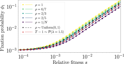
Figure 2: Fixation probability $\phi_{1}$ as a function of the mutant relative fitness advantage $s$ for $N=1000$. The dots correspond to numerical simulation results obtained from $10^{7}$ runs, and the lines to our theoretical predictions. Solid lines: constant sampling fraction $\rho$. Dashed black line: fluctuating sampling fraction drawn uniformly between $0$ and $1$ at each time step. Red dash-dotted line: fluctuating individual life time drawn from the law $T=1+X$ where $X$ follows a Poisson law with parameter $\lambda=1.5$.

Starting from one mutant, and assuming $s\ll 1$ while $Ns\gg 1$ and $N\gg 1$, Eq. 11 yields to leading order in $1/N$

$$\phi_{1}=\frac{2s}{2-\rho}\,.$$ (12)

We note that this is analogous to Haldane’s formula [21]

$$\phi_{1}=\frac{2s}{\sigma^{2}}\,,$$ (13)

where $\sigma^{2}=2-\rho$ is the variance of the number of offspring drawn from a Poissonian distribution (see SM [20] for details).

II.3 Rate of approach to steady state in the neutral case

In this section, we consider neutral mutants, i.e. $s=0$. The Markov chain representing the time evolution of the number of mutants in the population possesses two absorbing states, namely fixation and extinction of the mutant type. Therefore, the transition matrix in our model, whose elements are given by Eq. 4, has two unit eigenvalues [22]. The next largest non-unit eigenvalue provides information on the rate of decrease of genetic diversity in the population. It is thus of interest to calculate it. Denoting by $X_{t}$ be the number of mutant at time $t$, we can show that (see SM [20] for details)

$$\mathbb{E}\left[X_{t+1}(N-X_{t+1})|X_{t}\right] =X_{t}(N-X_{t})\lambda_{*}\,,$$ (14)

where, to leading order in $1/N$, we have:

$$\lambda_{*}=1-\frac{\rho(2-\rho)}{N}\,.$$ (15)

A theorem detailed in Appendix A of Ref.  [22] ensures that $\lambda_{*}$ is the highest non-unit eigenvalue of the transition matrix of the model.

The rate of approach to steady state is $\lambda_{*}$ for one event, i.e. for one discrete time step of the model [7]. Thus, for one generation, which corresponds to $1/\rho$ discrete time steps, it is, still to leading order in $1/N$,

$$r=\lambda_{*}^{1/\rho}=1-\frac{2-\rho}{N}\,.$$ (16)

Again, we recover both Moran and Wright-Fisher limits by taking $\rho=1/N$ and $\rho=1$, respectively [7, 23].

The convergence to steady state can be quantified by considering the vector $\bm{\pi}_{t}=(p_{0}(t),p_{1}(t),p_{2}(t),...,p_{N}(t))$ where $p_{k}(t)$ denotes the probability of having $k$ mutants at time $t$ starting from $1$ mutant at $t=0$. For $t\rightarrow\infty$, we have (see SM [20])

$$||\bm{\pi}_{t}-\bm{\pi}_{\infty}||_{2}\propto{\lambda_{*}}^{t}={r}^{\rho t}\,,$$ (17)

where $||.||_{2}$ refers to the Euclidean norm and $\bm{\pi}_{\infty}=\lim\limits_{t\rightarrow\infty}\bm{\pi}_{t}=(1-1/N,0,0,...,0,1/N)$. In Fig. 3, this prediction is tested numerically for different updated fractions $\rho$ of the population. We find a good agreement between our simulation results and the long-time asymptotic behavior given in Eq. 17.

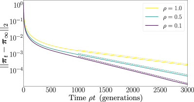
Figure 3: Approach to steady state in the neutral case. We show the Euclidean norm of $\bm{\pi}_{t}-\bm{\pi}_{\infty}$ (see main text) versus time in generations (i.e. rescaled with the generation time $1/\rho$), for $N=1000$ and with different updated fractions $\rho$. Full lines: simulation results obtained from $5.10^{7}$ runs. Dashed lines: asymptotic behavior given in Eq. 17, with a multiplicative constant chosen for legibility.

II.4 Effective population sizes

The effective population size is the size a regular Wright-Fisher population should have to match a given property of the population considered. It is of interest to express it for a population of size $N$ within our model.

Let us first consider the variance effective population size. Because the average generation time is $1/\rho$, the variance accumulated over one generation is $1/\rho$ times that in Eq. 10. Thus, the variance effective population size [3] within our model reads

$$N_{e}=\frac{x(1-x)}{\mathbb{V}(\Delta x)/\rho}=\frac{N}{2-\rho}.$$ (18)

Next, let us consider the eigenvalue effective population size. Eq. 16 allows us to express it as [3]

$$N_{e}=\frac{1}{1-r}=\frac{N}{2-\rho}\,.$$ (19)

We observe that these two effective population sizes coincide.

III Generalizations of the model

III.1 Fluctuating updated fraction

Let us extend our model where a fraction of the population is updated at each discrete time step to the case where the number $M$ of individuals selected to be updated can fluctuate. Let us assume that there is a probability $\pi^{(N)}(M)$ to have each value of $M$ between 0 and $N$. In a discrete time step of this new model, the transition probability is

$$P_{i\rightarrow j}^{\left(N,\pi^{(N)}\right)}=\sum_{M=0}^{N}\pi^{(N)}(M)P_{i\rightarrow j}^{(N,M)}\,,$$ (20)

where $P_{i\rightarrow j}^{(N,M)}$ is given by Eq. 4. To obtain the mutant fixation probability in the diffusion approximation within this new model, we express the first two moments of $\Delta x$. The calculation is similar to the one presented in SM [20] for the model with fixed updated fraction, and yields to leading order in $1/N$

$$\mathbb{E}(\Delta x) =\left<\rho\right>sx(1-x)\,,$$ (21)

$$\mathbb{V}(\Delta x) =\frac{\left<\rho(2-\rho)\right>}{N}x(1-x)\,,$$ (22)

where $\langle.\rangle$ denotes the average under the distribution $\pi^{(N)}$. Thus, the mutant fixation probability reads

$$\phi(x)=\frac{1-\exp\left(-\frac{2Nsx}{2-\langle\rho^{2}\rangle/\langle\rho\rangle}\right)}{1-\exp\left(-\frac{2Ns}{2-\langle\rho^{2}\rangle/\langle\rho\rangle}\right)}\,.$$ (23)

Starting from one mutant, and assuming $s\ll 1$ while $Ns\gg 1$ and $N\gg 1$, Eq. 23 yields to leading order in $1/N$

$$\phi_{1}=\frac{2s}{2-\left<\rho^{2}\right>/\left<\rho\right>}\,.$$ (24)

For instance, if $\pi^{(N)}$ is the uniform distribution between 0 and $N$, then we obtain $\phi_{1}=3s/2$ in this regime, which is the same prefactor as the one found for a constant update fraction $\rho=2/3$ (see Fig. 2). Furthermore, we note that

$$1\leq\frac{2}{2-\left<\rho^{2}\right>/\left<\rho\right>}\leq 2.$$ (25)

The first inequality follows from $\left<\rho^{2}\right>\geq 0$. Moreover, since $\forall\rho\in\left[0,1\right]$, $\rho^{2}\leq\rho$, we have $\left<\rho^{2}\right>\leq\left<\rho\right>$ for any $\pi^{(N)}$, yielding the second inequality. This result entails that the fixation probabilities in this model are comprised between those of the Moran and of the Wright-Fisher models.

Let us determine how $\rho$ is related to the lifetime of individuals $T$, i.e. to the number of time steps between two successive updates involving one given individual. The probability that a specific individual is selected to be updated at a given discrete time step is given by $M/N$, and $M$ is distributed according to $\pi^{(N)}$. Then, the probability that $T$ is equal to $k$ time steps, where $k$ is a positive integer, can be written as the probability that the individual of interest is not chosen at any of the $k-1$ previous updates and then is chosen, i.e.

$$p(T=k) =\left[\sum_{M=0}^{N}\pi^{(N)}(M)\frac{N-M}{N}\right]^{k-1}\sum_{M=0}^{N}\pi^{(N)}(M)\frac{M}{N}$$

$$=\left[1-\left<\rho\right>\right]^{k-1}\left<\rho\right>\,.$$ (26)

Thus, for any distribution $\pi^{(N)}$ of the fraction of the population chosen to be updated, the lifetime $T$ of an individual follows a geometric law with mean

$$\left<T\right> =\frac{1}{\left<\rho\right>}.$$ (27)

III.2 Fluctuating lifetimes

Let us now consider a different model, which is specified through the distribution $\pi_{\ell}$ of lifetimes of individuals. As before, the lifetime $T$ of an individual is intended as the time between two successive updates involving this individual. Time is still discrete, and thus $\pi_{\ell}(T=k)$ is defined over positive integers $k$. We assume that each of the $N$ individuals has the same distribution $\pi_{\ell}$ of lifetimes, and that they are all independent. In particular, mutants and wild-types have the same distribution $\pi_{\ell}$ of lifetimes. We further assume that there is no memory: a given lifetime is independent of previous ones, and all are identically distributed according to $\pi_{\ell}$. To relate this model to the previous ones, we aim to determine the distribution of the updated fraction $\rho$ from the lifetime distribution. Let us focus on the probability $p_{u}(t)$ for an individual to be updated at time $t$, which satisfies the equation

$$p_{u}(t)=\sum_{k=1}^{t}p_{u}(t-k)\pi_{\ell}(T=k)\,,$$ (28)

with the initial condition $p_{u}(t=0)=1$. Note that if $\pi_{\ell}$ is a geometric distribution, then its parameter is $1/\langle T\rangle$, and we obtain $p_{u}(t)=1/\left<T\right>$, which does not depend on $t$. This result is not always valid for other distributions. However, renewal process theory shows that it holds in the limit $t\rightarrow+\infty$ for many distributions [24, 25]:

$$\lim\limits_{t\rightarrow+\infty}p_{u}(t)=\frac{1}{\langle T\rangle}\,.$$ (29)

In this long-time limit, the distribution $\pi^{(N)}$ of the number $M$ of updated individuals is a binomial distribution $\mathcal{B}(N,p=1/\langle T\rangle)$, which leads to

$$\langle\rho\rangle=\frac{1}{\langle T\rangle}\,,$$ (30)

and we find to leading order in $1/N$

$$\frac{\langle\rho^{2}\rangle}{\langle\rho\rangle}=\frac{1}{\langle T\rangle}\,.$$ (31)

Eq. 24 then becomes

$$\phi_{1}=\frac{2s}{2-1/\left<T\right>}\,.$$ (32)

Again, this is consistent with Wright-Fisher and Moran models, indeed we have $\langle T\rangle=1$ in the Wright-Fisher model and $\langle T\rangle=N$ in the Moran model.

III.3 Selection on the lifetime

Let us now consider the case where mutants and wild-types have a different lifetime distribution. For simplicity, we start by neglecting selection on division, meaning that the Wright-Fisher update will be performed without selection, using the fraction $x$ of mutants and not its rescaled version $p$ (see Eq. 1). Concretely, let us assume that the lifetime of wild-types (resp. mutants) follows a geometric distribution with parameter $p_{w}$ (resp. $p_{m}=(1-s)p_{w}$). Note that $s$ still denotes the selection parameter, but it represents selection on lifetime here. Within this model, the transition probability can be written as

$$\begin{split}&P_{i\rightarrow j}^{(N,p_{m},p_{w})}=\sum_{M=0}^{N}\sum_{k=0}^{i}\binom{i}{k}p_{m}^{k}(1-p_{m})^{i-k}\\ &\quad\quad\quad\quad\times\binom{N-i}{M-k}p_{w}^{M-k}(1-p_{w})^{N-i-M+k}\\ &\quad\quad\quad\quad\times\binom{M}{k+j-i}x^{k+j-i}(1-x)^{M-k-j+i}\,.\end{split}$$ (33)

Indeed, each possible number $M$ of individuals chosen to be updated can be obtained by choosing $k$ mutants among $i$ according to their lifetime distribution, which is binomial (see above), and choosing $M-k$ wild-types among $N-i$ in a similar way. Finally, the Wright-Fisher update is performed for these $M$ chosen individuals, without selection.

Assuming as usual that $s$ is of order $1/N$, we obtain, to leading order in $1/N$ (see SM [20]):

$$\mathbb{E}(\Delta x) =p_{w}sx(1-x)\,,$$ (34)

$$\mathbb{V}(\Delta x) =\frac{p_{w}(2-p_{w})}{N}x(1-x)\,.$$ (35)

This allows us to express the fixation probability in the diffusion approximation as in other cases. In particular, assuming $s\ll 1$ while $Ns\gg 1$ and $N\gg 1$ it yields, to leading order in $1/N$,

$$\phi_{1}=\frac{2s}{2-p_{w}}=\frac{2s}{2-1/\langle T\rangle}\,,$$ (36)

where we used the fact that $p_{w}=1/\langle T\rangle$, with $\langle T\rangle$ the mean lifetime of individuals. Hence, the result takes the same form for selection on lifetime (death) as for selection on division (birth).

It is possible to generalize further by considering selection both on birth and death events. For this, we write $p_{m}=(1-s_{d})p_{w}$ and we perform Wright-Fisher sampling with parameters $m$ and $p=x(1+s_{b})/(1+xs_{b})$. Both $s_{d}$ and $s_{b}$ are assumed to be of order $1/N$. This case can be treated as above, yielding the fixation probability in the diffusion approximation. In particular, assuming $s_{d}\ll 1$ and $s_{b}\ll 1$ while $Ns_{d}\gg 1$, $Ns_{b}\gg 1$ and $N\gg 1$, it yields, to leading order in $1/N$,

$$\phi_{1}=\frac{2(s_{b}+s_{d})}{2-p_{w}}\,.$$ (37)

Note that for a Moran process with selection both on birth and death, the mutant fixation probability reads [10]

$$\phi_{1}=\dfrac{1-\dfrac{1-s_{d}}{1+s_{b}}}{1-\left(\dfrac{1-s_{d}}{1+s_{b}}\right)^{N}}\,.$$ (38)

In particular, assuming $s_{d}\ll 1$ and $s_{b}\ll 1$ while $Ns_{d}\gg 1$, $Ns_{b}\gg 1$ and $N\gg 1$, it yields, to leading order in $1/N$,

$$\phi_{1}=s_{b}+s_{d}\,,$$ (39)

which is consistent with Eq. 37 for $p_{w}=1/N$.

IV Discussion

We proposed a simple and tractable model that bridges the Wright-Fisher model and the Moran model. In our model, a fraction $\rho$ of the population is updated at each discrete time step, using binomial sampling. The Wright-Fisher model and the Moran model are recovered where the updated fraction $\rho$ is respectively $1$ and $1/N$. Under the diffusion approximation, we obtained the mutant fixation probability, as well as the rate of approach to steady state and the variance and eigenvalue effective population sizes. We further extended our model to the case where the updated fraction $\rho$ fluctuates. We derived a simple relation between the mean updated fraction and the mean individual lifetime. We considered the case where the lifetime fluctuates. Finally, we examined the situation where selection occurs both on birth and on death, assuming that the lifetime of individuals is geometrically distributed. In all these cases, we obtained simple expressions of the fixation probability in the diffusion approximation.

Our model can be seen as a particular case of the Chia and Watterson model [17]. We do not focus on the offspring distribution, but on the fraction of the population that is updated at each time step. This leads to a more tractable model where the Wright-Fisher and the Moran model emerge as simple limiting cases in the fixation probabilities.

Considering intermediate updated fractions has concrete applications, including bet-hedging strategies, where only a fraction of the population gives rise to the next generation, while the other seeds or offspring-generating individuals are dormant. These strategies allow the population to survive unpredictable or harsh environment changes. They are common in annual plants [26, 27], bacterial populations [28], and insects [29].

Here, we assumed discrete time steps, as in most classic models of population genetics. This is relevant in many situations, e.g. annual reproduction. Moreover, when continuous time is more relevant, as in bacterial reproduction, mutant replications remain synchronized for some time, as they stem from the same ancestor [30]. Besides, we focused on a well-mixed population with fixed size. It would be interesting to extend our model to spatially structured populations, or to fluctuations of the population size [31].

I Diffusion approximation

I.1 Simplified theorem from Ref. [1]

Justifying the diffusion approximation for population genetics models is a challenging topic in probability theory. The diffusion approximation was introduced in a seminal work by Kimura [3] and further formalized by Ethier and Nagylaki [1]. In Ref. [1], they considered Markov chains with two time scales. Here, we are interested in haploid individuals in a well-mixed population. Therefore, only one relevant timescale is involved, and we only need a simplified version of the theorem from Ref. [1], that we state below.

Let $x_{t}$ ($t=0,1,...$) be a homogeneous Markov chain in a metric space $E_{N}$ (where $N$ is the population size). Now let $\epsilon_{N}$ be a time scaling such that $\lim\limits_{N\rightarrow+\infty}\epsilon_{N}=0$. Let $x=x_{0}$ be the value of the initial state of the Markov chain. Assuming that the Markov chain has a transition function such that, $\forall x\in E_{N}$,

• $\epsilon_{N}^{-1}\mathbb{E}\left(\Delta x\right)=b(x)+o(1)$,

• $\epsilon_{N}^{-1}\mathbb{E}\left(\Delta x^{2}\right)=a(x)+o(1)$,

• $\epsilon_{N}^{-1}\mathbb{E}\left(\Delta x^{4}\right)=o(1)$.

where $\Delta x=x_{1}-x_{0}$. Then, provided some regularity assumptions on functions $a$ and $b$, $x_{[t/\epsilon_{N}]}$ (i.e. $x_{t}$ taken every $1/\epsilon_{N}$ steps) converges weakly to the diffusion process $x(\cdot)$ with generator:

$$\mathcal{L}=\dfrac{a(x)}{2}\dfrac{\partial^{2}}{\partial x^{2}}+b(x)\dfrac{\partial}{\partial x}.$$ (S1)

To apply this theorem to simple population genetics models, we need to write the mean and variance of the variation of the fraction of mutants, for one step of the Markov chain. Rescaling those functions by the appropriate time scaling $\epsilon_{N}$ should yield well-defined functions of order 1, while the fourth moment should be negligible. $\epsilon_{N}$ quantifies the scaling of the successive number of steps of the Markov chain that should be considered to obtain convergence to a diffusive process.

I.2 Application to simple population genetics models

Wright-Fisher model.

Consider the Wright-Fisher model with a fitness advantage $s$ of order $1/N$ of the mutant. Let us write $s=\alpha/N$ with $\alpha$ of order unity. The mean and variance of the variation of the mutant fraction $\Delta x$ read:

$$\mathbb{E}(\Delta x) =\dfrac{\alpha x(1-x)}{N}+o\left(\frac{1}{N}\right)\,,$$ (S2)

$$\mathbb{V}(\Delta x) =\dfrac{x(1-x)}{N}+o\left(\frac{1}{N}\right)\,.$$ (S3)

We can check that the fourth moment satisfies $\mathbb{E}\left(\Delta x^{4}\right)=\mathcal{O}(1/N^{2})$. Taking $\epsilon_{N}=1/N$, the assumptions of the theorem in the last section are satisfied, and thus $x_{[t/\epsilon_{N}]}$ converges weakly towards the diffusion process with generator

$$\mathcal{L}_{\text{WF}}=\dfrac{1}{2}x(1-x)\dfrac{\partial^{2}}{\partial x^{2}}+\alpha x(1-x)\dfrac{\partial}{\partial x}\,.$$ (S4)

Moran model.

For the Moran model,

$$\mathbb{E}(\Delta x) =\dfrac{\alpha x(1-x)}{N^{2}}+o\left(\frac{1}{N^{2}}\right)\,,$$ (S5)

$$\mathbb{V}(\Delta x) =\dfrac{2x(1-x)}{N^{2}}+o\left(\frac{1}{N^{2}}\right)\,,$$ (S6)

and we can check that the fourth moment is $\mathcal{O}(1/N^{3})$. This time, the right time scaling is $\epsilon_{N}=1/N^{2}$, and $x_{[t/\epsilon_{N}]}$ converges weakly to the diffusion process with generator

$$\mathcal{L}_{\text{Moran}}=x(1-x)\dfrac{\partial^{2}}{\partial x^{2}}+\alpha x(1-x)\dfrac{\partial}{\partial x}.$$ (S7)

I.3 Model with fixed updated fraction

Model.

In our model with fixed updated fraction, we pick $M$ individuals and update them as we update the single individual in the Moran model (in our description of the Moran model presented in the main text), considering the state of the whole population. The fraction of updated individuals is $\rho=M/N$. Setting $\rho=1/N$ yields the Moran model, while setting $\rho=1$ gives the Wright-Fisher model. As explained in the main text, the probability of transition from $i$ mutants to $j$ mutants is

$$P_{i\rightarrow j}^{(N,M)}=\sum_{k=0}^{i}\dfrac{\binom{i}{k}\binom{N-i}{M-k}}{\binom{N}{M}}\binom{M}{k+j-i}p^{k+j-i}(1-p)^{M+i-j-k}\,.$$ (S8)

Calculation of the first moments of $\Delta x$.

Let us determine the first two moments of the variation $\Delta X$ of the number of mutants in the first discrete time step, given that we start with $i$ mutants. First, let us compute the mean of $\Delta X$:

$$\mathbb{E}(\Delta X) =\sum_{k}\frac{\binom{i}{k}\binom{N-i}{M-k}}{\binom{N}{M}}\sum_{\Delta X}\Delta X\binom{M}{k+\Delta X}p^{k+\Delta X}(1-p)^{M-\Delta X-k}=\sum_{k}\frac{\binom{i}{k}\binom{N-i}{M-k}}{\binom{N}{M}}\left(Mp-k\right)$$

$$=Mp-\frac{1}{\binom{N}{M}}\sum_{k}\binom{i}{k}\binom{N-i}{M-k}k=Mp-i\frac{\binom{N-1}{M-1}}{\binom{N}{M}}=Mp-\frac{Mi}{N}=M(p-x)\,,$$ (S9)

where $x=i/N$. Second, let us compute its second moment:

$$\mathbb{E}(\Delta X^{2}) =\sum_{k}\frac{\binom{i}{k}\binom{N-i}{M-k}}{\binom{N}{M}}\sum_{\Delta X}\Delta X^{2}\binom{M}{k+\Delta X}p^{k+\Delta X}(1-p)^{M-\Delta X-k}$$

$$=\sum_{k}\frac{\binom{i}{k}\binom{N-i}{M-k}}{\binom{N}{M}}\sum_{j}(j-k)^{2}\binom{M}{j}p^{j}(1-p)^{M-j}$$

$$=Mp(1+p(M-1))-\frac{2Mp}{\binom{N}{M}}\sum_{k}\binom{i}{k}\binom{N-i}{M-k}k+\frac{1}{\binom{N}{M}}\sum_{k}\binom{i}{k}\binom{N-i}{M-k}k^{2}$$

$$=Mp(1+p(M-1))-2p\frac{iM^{2}}{N}+i(i-1)\frac{M(M-1)}{N(N-1)}+i\frac{M}{N}\,.$$ (S10)

These results allow us to determine the mean and variance of $\Delta x=\Delta X/N$. We have

$$\mathbb{E}(\Delta x)=\frac{\mathbb{E}(\Delta X)}{N}=\rho(p-x)\,,$$ (S11)

where $\rho=M/N$. Using the expression of $p$ given in Eq. 1 in the main text, and recalling that $s$ is assumed to be of order $1/N$, we obtain:

$$p-x=\frac{x(1+s)}{1+xs}-x=x\frac{s-xs}{1+xs}=s\frac{x(1-x)}{1+xs}=sx(1-x)+o\left(N^{-1}\right)\,,$$ (S12)

and hence

$$\mathbb{E}(\Delta x)=\rho sx(1-x)+o\left(\rho/N\right)\,.$$ (S13)

In addition, we have

$$\mathbb{E}(\Delta x^{2}) =\frac{\mathbb{E}(\Delta X^{2})}{N^{2}}=\frac{1}{N^{2}}\left[Mp(1+p(M-1))-2p\frac{iM^{2}}{N}+i(i-1)\frac{M(M-1)}{N(N-1)}+i\frac{M}{N}\right]$$

$$=\rho p\left[\frac{1}{N}+p\left(\rho-\frac{1}{N}\right)\right]-2px\rho^{2}+x\rho\left(x-\frac{1}{N}\right)\frac{\rho-N^{-1}}{1-N^{-1}}+\frac{\rho x}{N}\,.$$ (S14)

Since $p=x+sx(1-x)+o(1/N)$ (see Eq. S12), we find

$$\mathbb{E}(\Delta x^{2})=\frac{\rho(2-\rho)}{N}x(1-x)+o\left(\frac{\rho}{N}\right)\,,$$ (S15)

and thus the variance is

$$\mathbb{V}(\Delta x)=\frac{\rho(2-\rho)}{N}x(1-x)+o\left(\frac{\rho}{N}\right)\,.$$ (S16)

Diffusion limit.

We can check that the fourth moment of $\Delta x$ is $\mathcal{O}(\rho/N^{2})$. Taking the scaling $\epsilon_{N}=\rho/N$, $x_{[t/\epsilon_{N}]}$ converges weakly towards the diffusion process with generator

$$\mathcal{L}_{\rho}=\frac{\rho(2-\rho)}{2}x(1-x)\dfrac{\partial^{2}}{\partial x^{2}}+\alpha\rho x(1-x)\dfrac{\partial}{\partial x}.$$ (S17)

II Model with fixed updated fraction: leading non-unit eigenvalue

II.1 Derivation from the Chia and Watterson model and link with the variance of viable offspring

In Ref. [4], Chia and Watterson presented a population genetics model for a population with a fixed size of $N$ individuals. In this model, each individual produces offspring according to a probability law represented by a branching process with generating function $f$. At each discrete step $t$, a number $m$ is drawn from a probability distribution $p_{m}$, and $m$ individuals are sampled from the offspring pool, yielding a total pool of individuals is of size $N+m$. Then, the number $r$ of survivors is drawn from a probability distribution $q_{mr}$, and $r$ individuals are picked from the parents and $N-r$ from the $m$ offspring. The distributions $p_{m}$ and $q_{mr}$ are chosen such that $0\leq r\leq N\text{ and }0\leq N-r\leq m$. For completeness, below we summarize results from [4], and apply them to our partial sampling model.

Chia and Watterson computed all the eigenvalues of the transition matrix of the corresponding Markov process [4]. They also included a rate of mutation $\alpha_{1}$ from mutants to wild-types, and $\alpha_{2}$ for the opposite process. In the neutral case, the transition matrix element from $i$ to $j$ mutants in this model reads

$$P_{i\rightarrow j}=\sum_{m=0}^{\infty}\sum_{b=0}^{\infty}\sum_{r=0}^{\infty}p_{m}c_{mN}q_{mr}\text{ coefficient of }w^{m}z_{1}^{b}z^{j}\text{ in }\\ H(i,N-i,r,z)H(b,m-b,N-r,z)f^{i}((1-\alpha_{1})z_{1}w+\alpha_{1}w)f^{N-i}(\alpha_{2}z_{1}w+(1-\alpha_{2})w),$$ (S18)

where

$$H(i,N-i,r,z)=\sum_{k=0}^{\infty}z^{k}\dfrac{\binom{i}{k}\binom{N-i}{r-k}}{\binom{N}{r}},$$ (S19)

and $c_{mN}$ is the inverse of the coefficient of $z^{m}$ in $f^{N}(z)$. Focusing on the coefficient of $w^{m}$ means that we constrain the total offspring number to $m$. Focusing on the coefficient of $z_{1}^{b}$ means we are looking at cases in which the number of mutants within the offspring is $b$. Finally, focusing on the coefficient of $z^{j}$ means that the total number of mutants (among the population once it is updated) is $j$. The function $H(i,N-i,r,z)$ represents the ways of sampling $r$ individuals from a population of $N$ parents comprising $i$ mutants and $N-i$ wild-types. The function $H(b,m-b,N-r,z)$ represents the ways of sampling $N-r$ individuals from the $m$ offspring population made of $b$ mutants and $m-b$ wild-types. The function $f^{i}((1-\alpha_{1})z_{1}w+\alpha_{1}w)$ is the generating function for $i$ mutants, and $f^{N-i}(\alpha_{2}z_{1}w+(1-\alpha_{2})w)$ is the generating function for $N-i$ wild-types.

Application: partial sampling with fixed number of offspring and survivors.

Our partial sampling model can be seen as a particular case of the Chia and Watterson model, where we produce exactly the same number of offspring $M$ at each step, keep those $M$ individuals, and complete the new generation with $N-M$ individuals from the previous generation. This means that $p_{m}=1$ if $m=M$ and $0$ otherwise. We also have $q_{mr}=1$ if $r=N-M$, and 0 otherwise. We consider the no-mutation case where $\alpha_{1}=\alpha_{2}=0$. For the branching process representing offspring production, we use the Poisson law $\mathscr{P}(\mu)$ with generating function $f(z)=\exp(\mu(z-1))$. Let us write the transition matrix elements as $p_{ij}$, representing the probability of going from $i$ to $j$ mutants. We have

$$f^{i}(z_{1}w)f^{N-i}(w) =e^{-\mu N}\sum_{k}\dfrac{\mu^{k}}{k!}(iz_{1}w)^{k}\sum_{l}\dfrac{\mu^{l}}{l!}(N-i)^{l}w^{l},$$ (S20)

$$f^{N}(w) =e^{-\mu N}\sum_{k}\dfrac{\mu^{k}}{k!}w^{k}N^{k}.$$ (S21)

Computing the coefficient of $w^{m}z_{1}^{b}z^{j}$ in the expression given in Eq. S18 yields

$$\text{coef}=e^{-\mu N}\sum_{k=0}^{i}\frac{\binom{i}{k}\binom{N-i}{r-k}}{\binom{N}{r}}\frac{\binom{b}{j-k}\binom{m-b}{N-r-j+k}}{\binom{m}{N-r}}\frac{(i\mu)^{b}}{b!}\frac{\mu^{m-b}(N-i)^{m-b}}{(m-b)!},$$ (S22)

and we have

$$c_{mN}=\frac{m!\,e^{\mu N}}{(\mu N)^{m}}.$$ (S23)

Putting everything together with Eq. S18 yields

$$P_{i\rightarrow j}^{(N,M)}=\sum_{b=0}^{\infty}\sum_{k=0}^{i}\dfrac{\binom{i}{k}\binom{N-i}{N-M-k}}{\binom{N}{N-M}}\dfrac{\binom{b}{j-k}\binom{M-b}{M-j+k}}{\binom{M}{M}}\binom{M}{b}\left(\dfrac{i}{N}\right)^{b}\left(1-\dfrac{i}{N}\right)^{M-b}.$$ (S24)

Note that the parameter $\mu$ cancels out in this expression. Noticing that $\binom{b}{j-k}\binom{M-b}{M-j+k}$ is $1$ only if $b=j-k$ and $0$ otherwise, the equation simplifies, and we ultimately find

$$P_{i\rightarrow j}^{(N,M)}=\sum_{k=0}^{i}\dfrac{\binom{i}{k}\binom{N-i}{M-k}}{\binom{N}{M}}\binom{M}{k+j-i}\left(\dfrac{i}{N}\right)^{k+j-i}\left(1-\dfrac{i}{N}\right)^{M-k-j+i},$$ (S25)

which is the same as Eq. S8 in the neutral case.

Computing the relevant eigenvalue.

Chia and Watterson provided an explicit expression of all eigenvalues of the transition matrix for neutral mutants in Ref. [4]. Here, we are interested in the second largest eigenvalue $\lambda_{*}$ (the leading eigenvalue is equal to 1 and has multiplicity 2 when there are no mutations). Applying Chia and Watterson’s formula to our partial sampling model yields

$$\lambda_{*} =c_{MN}\binom{2}{0}\dfrac{(N-M)(N-M-1)}{N(N-1)}\text{ coeff. of }w^{M}\text{ in }f^{N}(w)$$

$$+c_{MN}\binom{2}{1}\dfrac{N-M}{N}\text{ coeff. of }w^{M-1}\text{ in }f^{\prime}(w)f^{N-1}(w)$$

$$+c_{MN}\binom{2}{2}\text{ coeff. of }w^{M-2}\text{ in }[f^{\prime}(w)]^{2}f^{N-2}(w).$$ (S26)

With a little algebra, we reach

$$\lambda_{*}=\dfrac{(N-M)(N-M-1)}{N(N-1)}+2\dfrac{(N-M)M}{N^{2}}+\dfrac{M(M-1)}{N^{2}},$$ (S27)

and substituting $M/N$ with $\rho$, we finally obtain:

$$\lambda_{*}=1-\dfrac{\rho(2-\rho)}{N}+o(1/N).$$ (S28)

Link with the variance of viable offspring.

Chia and Watterson define viable offspring as individuals that are part of the $m$ offspring at one generation, and that are kept to be part of the next generation, i.e. that are among the $N-r$ individuals sampled from the offspring. A viable individual has a life time which is geometrically distributed, and the mean lifetime is

$$\mu=\left[\sum_{m}\sum_{r}p_{m}q_{mr}\dfrac{N-r}{N}\right]^{-1}.$$ (S29)

Looking at the survival of one viable individual across several generations, we can write the generating function of its number of viable offspring $V$, $\phi(z)=\mathbb{E}[z^{V}]$. The detailed definition of this function is given in Ref. [4]. From this expression, we can derive that $\phi^{\prime}(1)=1$, which means that the average number of viable offspring produced by one individual is one, consistent with the fact that the population size remains constant. We can also derive the variance $\phi^{\prime\prime}(1)$ which appears in the eigenvalue $\lambda_{*}$ (see Ref. [4]) as

$$\lambda_{*}=1-\dfrac{\phi^{\prime\prime}(1)}{\mu(N-1)}.$$ (S30)

For our partial sampling model, the sums over $m$ and $r$ in the mean lifetime $\mu$ simplify and we get

$$\mu=\frac{N}{M}=\frac{1}{\rho}.$$ (S31)

From Eq. S30, and the expression of $\lambda_{*}$ in Eq. S28, we obtain for our partial sampling model $\phi^{\prime\prime}(1)=2-\rho$. From the diffusion approximation applied to the partial sampling model, and assuming $s\ll 1$ while $Ns\gg 1$ and $N\gg 1$, the fixation probability of one individual can be written as

$$\phi_{1}=\dfrac{2s}{2-\rho}.$$ (S32)

This is consistent with Haldane’s expression of the fixation probability which reads $\phi_{1}=2s/\sigma^{2}$, where $\sigma^{2}$ is the variance of the offspring, and thus is equal to $\phi^{\prime\prime}(1)=2-\rho$.

II.2 Derivation of the leading non-unit eigenvalue using Ref. [2]

Here, we present another method proposed in [2] to compute the leading non-unit eigenvalue $\lambda_{*}$ of the transition matrix for the partial sampling model in the neutral case. The key result is that, if there exists a function $f$ such that $\mathbb{E}[f(X_{t+1})|X_{t}]=af(X_{t})$ where $a$ is a constant, then $a=\lambda_{*}$ is the desired eigenvalue [2]. Taking $f(X)=X(N-X)$ for our partial sampling model yields

$$\mathbb{E}(X_{t+1}|X_{t}) =X_{t}\,$$ (S33)

$$\mathbb{E}\left[X_{t+1}(N-X_{t+1})|X_{t}\right] =\mathbb{E}\left[(X_{t}+\Delta X)(N-X_{t}-\Delta X)|X_{t}\right]$$

$$=X_{t}(N-X_{t})-\mathbb{E}(\Delta X^{2}|X_{t})$$

$$=X_{t}(N-X_{t})\left[1-\frac{\rho(2-\rho)}{N}+o\left(\frac{1}{N}\right)\right],$$ (S34)

where we used the fact that $\mathbb{E}(\Delta X)=0$ in the neutral case, and the expression of $\mathbb{E}(\Delta X^{2})$ from Eq. S10. Therefore, we can identify

$$\lambda_{*}=1-\frac{\rho(2-\rho)}{N}+o\left(\frac{1}{N}\right),$$ (S35)

which matches the result obtained in Eq. S28 using the Chia and Watterson model.

II.3 Rate of approach to the stationary state

The largest non-unit eigenvalue $\lambda_{*}$ of the transition matrix $\bm{P}=\left\{P_{i\rightarrow j}\right\}_{ij}$ quantifies the rate of convergence towards the stationary state. Concretely, let us consider the vector $\bm{\pi}_{t}=(p_{0}(t),p_{1}(t),p_{2}(t),...,p_{N}(t))$ where $p_{k}(t)$ denotes the probability of having $k$ mutants at time $t$ starting from $1$ mutant at $t=0$. This vector satisfies

$$\bm{\pi}_{t+1}=\bm{P}\,\bm{\pi}_{t}\,,$$ (S36)

with $\bm{\pi}_{0}=(0,1,0,0,...,0)$ at time $t=0$. We can decompose this vector in the basis of eigenvectors of $\bm{P}$ written $\bm{u}_{k}$:

$$\bm{\pi}_{0}=\sum_{k=0}^{N}a_{k}\bm{u}_{k}\,,$$ (S37)

where we introduced coefficients $a_{k}$. At time step $t$, we have

$$\bm{\pi}_{t}={\bm{P}}^{t}\bm{\pi}_{0}=\sum_{k=0}^{N}a_{k}{\lambda_{k}}^{t}\bm{u}_{k}\,,$$ (S38)

where $\lambda_{0}=\lambda_{1}=1$, due to the two absorbing states (extinction and fixation of the mutants) and $0<\lambda_{k}<1$ for $k\geq 2$. When $t\rightarrow+\infty$, we obtain

$$\lim\limits_{t\rightarrow+\infty}\bm{\pi}_{t}=\bm{\pi}_{\infty}=a_{0}\bm{u}_{0}+a_{1}\bm{u}_{1}\,,$$ (S39)

where $\bm{\pi}_{\infty}=(1-1/N,0,0,...,0,1/N)$. We can thus write

$$\bm{\pi}_{t}=\bm{\pi}_{\infty}+a_{2}{\lambda_{*}}^{t}\bm{u}_{2}+\sum_{k=3}^{N}a_{k}{\lambda_{k}}^{t}\bm{u}_{k}$$ (S40)

By taking the Euclidean norm $||\bm{\pi}_{t}-\bm{\pi}_{\infty}||_{2}$ of the difference between $\bm{\pi}_{t}$ and $\bm{\pi}_{\infty}$, we find

$$||\bm{\pi}_{t}-\bm{\pi}_{\infty}||_{2}={\lambda_{*}}^{t}a_{2}||\bm{u}_{2}||_{2}+\sum_{k=3}^{N}{\lambda_{k}}^{t}a_{k}||\bm{u}_{k}||_{2}\,.$$ (S41)

In the long-time limit, the dominant term is the one involving $\lambda_{*}$. Thus, for $t\rightarrow\infty$,

$$||\bm{\pi}_{t}-\bm{\pi}_{\infty}||_{2}\propto{\lambda_{*}}^{t}={r}^{\rho t}\,,$$ (S42)

where $r={\lambda_{*}}^{1/\rho}$ (see Eq. 16 in the main text).

III Model with selection on the lifetime: first moments of $\Delta x$

In this section, we compute the mean and variance of $\Delta x=\Delta X/N$ in a model with selection on the life time of individuals. In this model, we assume that the lifetime of wild-types (resp. mutants) is geometrically distributed with parameter $p_{w}$ (resp. $p_{m}=(1-s)p_{w}$), where $s$ denotes the selection parameter. The transition matrix is given in Eq. 33 of the main text. Using the same notations as in Section I above, the mean of $\Delta X$ reads

$$\mathbb{E}(\Delta X) =\sum_{k,m}\binom{i}{k}p_{m}^{k}(1-p_{m})^{i-k}\binom{N-i}{m-k}p_{w}^{m-k}(1-p_{w})^{N-i-m+k}\sum_{\Delta X}\binom{m}{k+\Delta X}x^{k+\Delta X}(1-x)^{m-k-\Delta X}\Delta X$$

$$=\sum_{k}\binom{i}{k}p_{m}^{k}(1-p_{m})^{i-k}\sum_{m}\binom{N-i}{m-k}p_{w}^{m-k}(1-p_{w})^{N-i-m+k}(mx-k)$$

$$=\sum_{k}\binom{i}{k}p_{m}^{k}(1-p_{m})^{i-k}(xp_{w}(N-i)-k(1-x))$$

$$=xp_{w}(N-i)-(1-x)p_{m}i=Nx(1-x)(p_{w}-p_{m})$$

$$=Np_{w}sx(1-x)\,.$$ (S43)

Meanwhile, the second moment is

$$\mathbb{E}(\Delta X^{2}) =\sum_{k,m}\binom{i}{k}p_{m}^{k}(1-p_{m})^{i-k}\binom{N-i}{m-k}p_{w}^{m-k}(1-p_{w})^{N-i-m+k}\sum_{\Delta X}\binom{m}{k+\Delta X}x^{k+\Delta X}(1-x)^{m-k-\Delta X}\Delta X^{2}$$

$$=\sum_{k}\binom{i}{k}p_{m}^{k}(1-p_{m})^{i-k}\sum_{m}\binom{N-i}{m-k}p_{w}^{m-k}(1-p_{w})^{N-i-m+k}\left\{m^{2}x^{2}+m\left[x(1-x)-2kx\right]+k^{2}\right\}$$

$$=\sum_{k}\binom{i}{k}p_{m}^{k}(1-p_{m})^{i-k}\left\{x^{2}\left[(N-i)^{2}p_{w}^{2}+(N-i)p_{w}(1-p_{w})\right]+x(1-x)(N-i)p_{w}(1-2k)\right.$$

$$\left.+kx(1-x)+k^{2}(1-x)^{2}\right\}$$

$$=x^{2}\left[(N-i)^{2}p_{w}^{2}+(N-i)p_{w}(1-p_{w})\right]+x(1-x)(N-i)p_{w}$$

$$+x(1-x)(1-2p_{w}(N-i))ip_{m}+(1-x)^{2}\left[i^{2}p_{m}^{2}+ip_{m}(1-p_{m})\right]\,.$$ (S44)

Finally, to first order in $1/N$, the mean and variance of $\Delta x=\Delta X/N$ read

$$\mathbb{E}(\Delta x) =p_{w}sx(1-x)+o\left(N^{-1}\right)\,,$$ (S45)

$$\mathbb{V}(\Delta x) =\frac{p_{w}(2-p_{w})}{N}x(1-x)+o\left(N^{-1}\right)\,.$$ (S46)

References

- [1] Fisher, R. The genetical theory of natural selection. (1930).
- [2] Wright, S. Evolution in mendelian populations. Genetics 16, 97 (1931).
- [3] Ewens, W. On the concept of the effective population size. Theoretical Population Biology 21, 373–378 (1982).
- [4] Tataru, P., Simonsen, M., Bataillon, T. & Hobolth, A. Statistical Inference in the Wright–Fisher Model Using Allele Frequency Data. Systematic Biology 66, e30–e46 (2016).
- [5] Tataru, P., Bataillon, T. & Hobolth, A. Inference under a Wright-Fisher model using an accurate beta approximation. Genetics 201, 1133–1141 (2015).
- [6] Paris, C., Servin, B. & Boitard, S. Inference of selection from genetic time series using various parametric approximations to the Wright-Fisher model. G3: Genes, Genomes, Genetics 9, 4073–4086 (2019).
- [7] Moran, P. A. P. Random processes in genetics. In Mathematical Proceedings of the Cambridge Philosophical Society, vol. 54, 60–71 (Cambridge University Press, 1958).
- [8] Lieberman, E., Hauert, C. & Nowak, M. A. Evolutionary dynamics on graphs. Nature 433, 312–316 (2005).
- [9] Hindersin, L. & Traulsen, A. Most undirected random graphs are amplifiers of selection for birth-death dynamics, but suppressors of selection for death-birth dynamics. PLoS Computational Biology 11, e1004437 (2015).
- [10] Kaveh, K., Komarova, N. L. & Kohandel, M. The duality of spatial death–birth and birth–death processes and limitations of the isothermal theorem. Royal Society Open Science 2, 140465 (2015).
- [11] Marrec, L., Lamberti, I. & Bitbol, A.-F. Toward a universal model for spatially structured populations. Physical Review Letters 127, 218102 (2021).
- [12] Taylor, C., Fudenberg, D., Sasaki, A. & Nowak, M. A. Evolutionary game dynamics in finite populations. Bulletin of Mathematical Biology 66, 1621–1644 (2004).
- [13] Nowak, M. A., Sasaki, A., Taylor, C. & Fudenberg, D. Emergence of cooperation and evolutionary stability in finite populations. Nature 428, 646–650 (2004).
- [14] Ohtsuki, H. & Nowak, M. A. The replicator equation on graphs. Journal of Theoretical Biology 243, 86–97 (2006).
- [15] Karlin, S. & McGregor, J. Direct product branching processes and related markov chains. Proceedings of the National Academy of Sciences 51, 598–602 (1964).
- [16] Karlin, S. & Mc Gregor, J. Direct product branching processes and related induced markoff chains i. calculations of rates of approach to homozygosity. In Bernoulli 1713, Bayes 1763, Laplace 1813: Anniversary Volume. Proceedings of an International Research Seminar Statistical Laboratory University of California, Berkeley 1963, 111–145 (Springer, 1965).
- [17] Chia, A. & Watterson, G. Demographic effects on the rate of genetic evolution I. Constant size populations with two genotypes. Journal of Applied Probability 6, 231–248 (1969).
- [18] Cannings, C. The equivalence of some overlapping and non-overlapping generation models for the study of genetic drift. Journal of Applied Probability 10, 432–436 (1973).
- [19] Kimura, M. On the probability of fixation of mutant genes in a population. Genetics 47, 713 (1962).
- [20] See Supplemental Material for further details.
- [21] Boenkost, F., Gonzalez Casanova, A., Pokalyuk, C. & Wakolbinger, A. Haldane’s formula in cannings models: the case of moderately weak selection (2021).
- [22] Ewens, W. J. Population Genetics (Springer Science & Business Media, 2013).
- [23] Cannings, C. The latent roots of certain markov chains arising in genetics: a new approach, i. haploid models. Advances in Applied Probability 6, 260–290 (1974).
- [24] Erdös, P., Feller, W. & Pollard, H. A property of power series with positive coefficients (1949).
- [25] Feller, W. Fluctuation theory of recurrent events. Transactions of the American Mathematical Society 67, 98–119 (1949).
- [26] Venable, D. L. Bet hedging in a guild of desert annuals. Ecology 88, 1086–1090 (2007).
- [27] Gremer, J. R. & Venable, D. L. Bet hedging in desert winter annual plants: optimal germination strategies in a variable environment. Ecology Letters 17, 380–387 (2014).
- [28] Veening, J.-W. et al. Bet-hedging and epigenetic inheritance in bacterial cell development. Proceedings of the National Academy of Sciences 105, 4393–4398 (2008).
- [29] Joschinski, J. & Bonte, D. Diapause and bet-hedging strategies in insects: a meta-analysis of reaction norm shapes. Oikos 130, 1240–1250 (2021).
- [30] Jafarpour, F., Levien, E. & Amir, A. Evolutionary dynamics in non-markovian models of microbial populations. Physical Review E 108, 034402 (2023).
- [31] Engen, S., Lande, R. & Saether, B.-E. Effective size of a fluctuating age-structured population. Genetics 170, 941–954 (2005).
Supplemental Material for “Bridging Moran and Wright-Fisher models”
Arthur Alexandre, Alia Abbara, Cecilia Fruet, Claude Loverdo, Anne-Florence Bitbol

References

- [1] Ethier, S. N. & Nagylaki, T. Diffusion approximations of Markov chains with two time scales and applications to population genetics. Advances in Applied Probability 12, 14–49 (1980).
- [2] Ewens, W. J. Population Genetics (Springer Science & Business Media, 2013).
- [3] Kimura, M. On the probability of fixation of mutant genes in a population. Genetics 47, 713 (1962).
- [4] Chia, A. & Watterson, G. Demographic effects on the rate of genetic evolution I. Constant size populations with two genotypes. Journal of Applied Probability 6, 231–248 (1969).