Two methods to analyse radial diffusion ensembles: the peril of space- and time- dependent diffusion

Abstract

Particle dynamics in Earth’s outer radiation belt can be modelled using a diffusion framework, where large-scale electron movements are captured by a diffusion equation across a single adiabatic invariant, $L^{*}$ $``(L)"$. While ensemble models are promoted to represent physical uncertainty, as yet there is no validated method to analyse radiation belt ensembles. Comparisons are complicated by the domain dependent diffusion, since diffusion coefficient $D_{LL}$ is dependent on $L$. We derive two tools to analyse ensemble members: time to monotonicity $t_{m}$ and mass/energy moment quantities $\mathcal{N},\mathcal{E}$. We find that the Jacobian ($1/L^{2}$) is necessary for radiation belt error metrics. Components of $\partial\mathcal{E}/\partial t$ are explicitly calculated to compare the effects of outer and inner boundary conditions, and loss, on the ongoing diffusion. Using $t_{m}$, $\mathcal{N}$ and $\mathcal{E}$, we find that: (a) different physically motivated choices of outer boundary condition and location result in different final states and different rates of evolution; (b) the gradients of the particle distribution affect evolution more significantly than $D_{LL}$; (c) the enhancement location, and the amount of initial background particles, are both significant factors determining system evolution; (d) loss from pitch-angle scattering is generally dominant; it mitigates but does not remove the influence of both initial conditions and outer boundary settings, which are due to the $L$-dependence of $D_{LL}$. We anticipate this study will promote renewed focus on the distribution gradients, on the location and nature of the outer boundary in radiation belt modelling, and provide a foundation for systematic ensemble modelling.

I Introduction

Radial diffusion is a phenomenon studied in both space and fusion plasmas. In this work, we investigate how the radial dependence of that diffusion interacts with initial and boundary conditions. We provide here a guide for different readers to navigate this paper. Firstly, in the introduction we provide a broad introduction of the motivations behind understanding the uncertainty in radial diffusion modelling in near-Earth space. Plasma physicists without a radiation belt background may wish to review the application of radial diffusion in near-Earth space in Section II. For all readers, we explicitly list our goals in Section III, introducing labels which are used throughout the manuscript as we develop each research question, find relevant results and then discuss our conclusions. Section IV contains details of the numerical models and develops the properties we require in an analysis metric, thereby motivating our use of time to monotonicity and the mass- and energy-like quantities $\mathcal{N},\mathcal{E}$. We find and present the most significant ways in which these quantities vary in Section V. Radiation belt modellers and space weather physicists may be particularly interested in the suggestions we make for future based on our findings in Section VI, where we also compare our results to current modelling practices. Some of our more significant conclusions relate to the importance of the outer boundary and the particle gradients instead, which are also discussed in Section VI. Where possible, each section is self-contained, to enable those with different interests to find the relevant sections useful.

Earth’s radiation belts are a region of highly energised particles, magnetically trapped by the Earth’s magnetosphere. The trapped particles undergo several types of periodic motion, the slowest of these being the drift around the Earth. Electromagnetic perturbations on timescales of the drift of electrons around the Earth will scatter those electrons onto orbits closer to, or more distant from, the Earth; this is radial diffusion. Radial diffusion is one of the major drivers of Earth’s radiation belts and due to the variation in timescales of radiation belt particles motions, an approximation for radiation belt modelling can be made using solely this mechanism . This simple yet effective model enables us to explore ways of including uncertainty in our radiation belt models using ensembles. A full model of the radiation belts would require us to acknowledge that they are part of a complex, interdependent system, with consequently larger amounts of uncertainty. Radial diffusion modelling using the Fokker-Planck formalism is reviewed in more detail in Section II; briefly, radiation belt modelling does not use the motion of individual particles but instead averages over motion on larger scales, where wave-particle interactions across many scales are included using diffusion coefficients. Where the wave-particle interactions are well understood, variability should be properly characterised in order to capture the correct uncertainty. Where these interactions are not well understood, uncertainty across orders of magnitude can indicate inadequate modelling. For example, estimates of $D_{LL}$ under similar conditions vary by orders of magnitude [Huang2010b,Liu2016,Thompson2020,Sarma2020]

Ensembles can be used to quantify uncertainty in radiation belt modelling. Ensemble modelling involves running a simulation multiple times, with a variety of input conditions or parameter settings, to represent the unknowns in a given system. The impact of these unknowns on the final state can be quantified; alternatively, variability across model outputs provide a measure of uncertainty on that final state. Probability distribution of model outputs provide us with a better understanding of the uncertainty associated with our models. There are several sources of uncertainty in radiation belt modeling, including uncertainty due to approximations or physical unknowns, uncertainty in observations (i.e. in the measured value and in the spacecraft location), uncertainty in boundary conditions or model settings and physical uncertainty inherent to the system. Physical uncertainty arises from the fact that deterministic models may exhibit chaotic behaviour if they are particularly sensitive to initial conditions. Given that the magnetosphere is a complex system and that we have very sparse observations, it is extremely likely that we will need some way to include this chaotic deterministic character. Furthermore, the computational requirements of our modelling mean that we have sub-grid physics: physics on smaller scales that must be included, but cannot be fully modelled numerically. Uncertainty in driving parameters, such as upscale solar wind and ultra-low-frequency waves driving radial diffusion, can also affect the accuracy of the model. As radiation belt modelling improves, it becomes increasingly important to understand how all of these sources of uncertainty impact our final output to be able to analyse ensembles.

As uncertainty becomes increasingly important in radiation belt modelling, methods to account for uncertainty such as data assimilation and statistical methods are becoming the state-of-the-art method for modeling radiation belts, while complex systems approaches are being applied to understand the underlying physics Balasis et al. (2023). Morley (2020) states that the field of space physics needs ensembles and methods to deal with and analyse ensembles, in order to manage uncertainty in parameterisations and in various parts of numerical space weather prediction. Ensembles, and other probabilistic methods, are already becoming the norm Hua et al. (2023); Watt et al. (2022); Sarma et al. (2020); Shprits et al. (2013).

Satellite operators and national meteorological organisations are increasingly compelled to include space weather forecasting as part of their services, including the radiation environment. Geomagnetically trapped particles in the radiation belts have been established as a hazard to spacecraft due to processes such as surface charging, deep dielectric charging and single upset events Hands et al. (2018); Matéo-Vélez et al. (2018). The loss of services such as the internet would cause severe socio-economic issues such as losses to navigation, finances (including card-based payments) and tracking/allocation of emergency services and commercial aircraft. These economic motivations for adapting modelling this fascinating system have also encouraged the space plasma physics community to adopt techniques mastered by meteorologists. However, the domain dependence of the diffusion coefficient means that using and analysing ensemble members is not simple, rendering ensembles less meaningful than desired.

To understand ensemble models for radial diffusion (and for radiation belt modelling more generally) we need to understand how simple model changes and initial and boundary conditions change the outputs, before we include variability to represent uncertainty in physical conditions.

II Background: Radial Diffusion Modelling in Earth’s Radiation Belts

Radiation belt modelling is typically done using three adiabatic invariants; three quantities associated with the periodic motions of trapped, highly charged particles in Earth’s magnetosphere. At relatively low energies (e.g. electrons of 1-100s of keV), particles are better described using the ring current paradigm. At higher energies (e.g. relativistic electrons $\geq 0.5$ MeV) we use the geomagnetically trapped radiation belt description Roederer and Zhang (2014); Walt (2005). Periodic motions of particles in a slowly changing conservative field (such as electromagnetic fields) correspond to conserved quantities; adiabatic invariants. The first adiabatic invariant, $\mu$, corresponds to the magnetic moment as particles gyrate in an electromagnetic field. The second invariant corresponds to momentum along the bounce path, as the gyrating particle travels up and down the field line, reflected by the stronger magnetic field “magnetic bottle"). These motions are on scales of microseconds and seconds, respectively. Under the adiabatic approximation, if the system is changing slowly, then these quantities are conserved. On the other hand, if the system is perturbed on timescales comparable to these motions, the quantities $\mu$ or $J$ would not be conserved. On a much longer timescale, the periodic motion of electrons drifting around the Earth corresponds to the third adiabatic invariant $\Phi$, the magnetic flux enclosed by this drift path. This can be written as $\Phi=2\pi B_{0}\frac{R_{E}^{3}}{R_{0}}$ for particles remaining at the equator, with $R_{0}$ the equatorial distance, $B_{0}$ the magnetic field strength at the Earth’s surface and $R_{E}$ the radius of the Earth. One can therefore model the radiation belts using these conserved quantities, by tracking the distribution of particles in this adiabatic invariant space and assuming that the change in this space can be modelled using diffusion - where diffusion between these occurs when electromagnetic perturbations occur on the temporal and spatial scales of the corresponding periodic motions. Diffusion is described using diffusion coefficients $D_{\alpha\beta}$. Typically, cross-terms corresponding to the third adiabatic invariant are considered to be zero; on the whole, changes to the thrid adiabatic invariant ("radial diffusion") is considered to be on a separate timescale and can therefore be approximated alone (e.g. Reeves et al. (2012)). The full diffusion model of the radiation belts has been used in a number of places, e.g. Beutier and Boscher (1995); Glauert et al. (2014); Subbotin and Shprits (2009); Reeves et al. (2012).

For the third adiabatic invariant, one can equivalently consider the drift shells instead of the magnetic flux conserved by the drift orbit. Since the drift shell is uniquely defined by its intersection with the equatorial magnetic field, it is often easier and more intuitive to parameterise the third adiabatic invariant using some form of $L^{*}$ parameter, which roughly translates to which nested drift shell a given electron is confined to. (From this point on we will refer to $L$-parameters, rather than $L^{*}$, for simplicity in notation). The drift shells a given $L$ correspond to will depend on the specific magnetic field model used, and multiple methods of defining $L$ exist depending on both the magnetic field and the approximations used to specify the drift shells (see e.g. Thompson et al. (2021); Lejosne and Albert (2023); Walt (2005); Roederer and Zhang (2014)). If one considers the $L$ parameter as a proxy for the relative radius of each drift shell, it becomes clear why diffusion across the third adiabatic invariant is called "radial diffusion": particles diffusing to different $L$ values are diffusing onto drift shells closer to, or further from the Earth. On the whole, radial diffusion is related to the large scale movement of particles towards and away from the Earth, acting to reduce gradients in the phase space density profile. The inward diffusion also corresponds to an increase in energy, if the first adiabatic invariant is conserved. Meanwhile, smaller scale processes breaking the first and second adiabatic invariants result in local acceleration of particles (e.g. Green and Kivelson (2004); Reeves et al. (2013)).

The diffusion coefficient $D_{LL}$ contains the combined effect of electromagnetic perturbations on timescales corresponding to the electron drift. These perturbations consequently break the third adiabatic invariant, causing the diffusion to nearby $\Phi$ (or, equivalently, $L$). A comprehensive review of the current state of knowledge of radial diffusion coefficients can be found in Lejosne and Kollmann (2020). The first attempts to quantify this into a diffusion coefficient $D_{LL}$ assumed that such perturbations were stochastic; small scale continual ripples in the magnetosphere. The contributions from magnetic and electric potential perturbations were considered separately, using asymmetric and symmetric perturbations from a simple magnetic field model Falthammar (1968). Unfortunately these theoretical diffusion coefficients are problematic to apply; the magnetosphere is significantly more dynamic, rendering these assumptions invalid, while in practice one cannot observe these quantities to estimate them more accurately. There exists a gap between the theory and application of radial diffusion; accurate diffusion coefficients would require knowledge of the entire magnetosphere at each timestep to be able to calculate electron drift paths. Theoretical approaches must use magnetic field models and tend to focus on determining the validity of the underlying assumptions in order to derive a more appropriate method of calculating diffusion coefficients Lejosne (2019); Osmane and Lejosne (2021); Lejosne and Albert (2023). Any estimations of $D_{LL}$ used in modelling must make a significant number of approximations, most often based on the techniques in Brautigam et al. (2005); Fei et al. (2006) (particularly operational models).

Fei et al. (2006) derives the diffusion coefficients for a particular storm using a formalism based on Falthammar (1968): for a given magnetic field model, find the deviation $\frac{dL}{dt}$ from drift contours due to azimuthally symmetric and asymmetric electromagnetic perturbations, and from this find $\left<(\Delta L)^{2}\right>$ and hence $D_{LL}.$ Fei et al. (2006) uses a compressed dipole magnetic field, using an asymmetry factor $\Delta B$. Fei et al. (2006) also splits the diffusion coefficients into diffusion due to magnetic and electric perturbations, rather than into perturbations from induced electric and electric potential fields. Fei et al. (2006) used the larger component of the two to avoid counting the effect of the same perturbation twice, but the component which was dominant during their case study is not always the strongest one Olifer et al. (2019); Sandhu et al. (2021). In many subsequent studies, these components are simply added together to estimate $D_{LL}$. This makes the diffusion coefficients much easier to find and apply, but the resultant double-counting of perturbations means the final values could be off by around a factor of 2 Lejosne (2019). Given that the uncertainty in $D_{LL}$ across different methods in similar situations spans orders of magnitudes Huang et al. (2010); Liu et al. (2016); Olifer et al. (2019); Sandhu et al. (2021), this double-counting is considered an acceptable compromise. Other choices made by Fei et al. (2006) based on properties of their storm-time magnetosphere are also replicated in subsequent methods, simply to have any ability to model the radiation belts at all. This may be why so many of these methods perform similarly - well on average, but with little specificity. A list of sources of uncertainty in $D_{LL}$ can be found in Bentley et al. (2019).

III Research Goals

Here we pause to explicitly identify research goals. Having a separate section for this allows us to report back on unfruitful research avenues and to directly label our goals to conclusion in the discussion, making the logic easy to navigate across several key results. No research paper has only a single important result and we hope this will bring out subtleties that may otherwise be missed.

We split these research goals up into:

1. Primary goals (research questions identified when scoping out the the project and applying for funding)

2. Secondary goals (research questions that arose when developing our methodology)

3. Additional goals (further questions that arose as part of the analysis which we realised can answer as part of this work)

We choose to present our work in this way as it reflects our cylic methodology far more accurately, where we constantly revisited concepts and experiments until we reached a coherent structure explaining our results.

III.1 Primary Goals

1. Benchmarking for ensembles.

   1. How does one analyse ensembles for radiation belt modelling? How can we quantify differences between ensemble runs?

   2. Do changes in initial condition affect the differences between ensemble members? If so, which aspects of the initial condition have the strongest impacts?

   3. Do changes in model settings (such as $L_{outer}$) affect the differences between ensemble members?

2. What is the timescale of radial diffusion?

   1. What is a useful definition of “timescale"?

   2. What is the general radial diffusion timescale?

   3. Does timescale vary with initial conditions?

III.2 Secondary Goals

1. What do we do if we are not using a data-driven outer boundary?

   1. What boundary conditions would be physical to use? (rather than what is convenient for our observations)

   2. Where there are multiple potentially physical boundary conditions, how do they affect the timescale and evolution of radial diffusion?

   3. What conditions should we use in future?

   4. How does the choice of outer boundary condition and location interact with the current uncertainty on the outer boundary of radiation belt models?

   5. How does the outer boundary location interact with the increased diffusion coefficient at high $L$?

2. What happens to an enhancement from local acceleration under radial diffusion (rather than just inwards diffusion of the “background” distribution, i.e. a source at high $L$?)

3. How can time to monotonicity/ morphology of the particle distribution be used to analyse ensemble members?

4. Do we need to include loss to represent radial diffusion?

III.3 Additional Goals

1. What analytical methods can be adapted to understand radial diffusion?

2. How important are gradients vs the $L$-dependence of $D_{LL}$?

3. Is diffusion limited by the smallest value of $D_{LL}$ in the domain, i.e. the diffusion coefficient at lower $L$?

In the Section VI we will discuss our findings for each of these questions and outline future questions that are unanswered.

IV Methods

In this section we will outline the scheme used for the numerical experiments in our ensemble and the metrics we use to analyse our experiments. We choose not to compare variability across the final phase space density distributions after a set time period, but to compare how several useful quantities vary across ensemble members. We use a proxy (time to monotonicity, $t_{m}$) that indicates when radial diffusion has finished changing the shape of the distribution, and mass-like and energy-like techniques from analysis of dynamical systems to understand the ongoing evolution of the distribution. These tools allow us to see how radial diffusion is still contributing to radiation belt dynamics.

In Section IV.1 we discuss our equation for the initial condition, the parameters we will vary in our ensemble and the diffusion model we use. In Section IV.2 we will motivate time to monotonicity as a metric for timescale. In Section IV.3 we derive the energy density-like and mass-like quantities we use to verify and interpret our simulations.

Results from our investigation can be found in Section V and are brought into context with current understanding in Section VI.

IV.1 Numerical Experiments

IV.1.1 The Diffusion Model

Although the full diffusion equation for the radiation belts models the phase space density (PSD) of electrons across all three adiabatic invariants, $M,J,\Phi$, the vastly longer timescales of drift motion means that one can separate out radial diffusion. We simulate radial diffusion following Thompson et al. (2020). An idealised model allows us to examine how variation in initial conditions affect the final distributions, due solely to our modelling (rather than, for example, time-varying coefficients or inputs). We solve the radial diffusion equation

$$\frac{\partial f(M,J,\Phi)}{\partial t}=L^{2}\frac{\partial}{\partial L}\left(\frac{D_{LL}}{L^{2}}\frac{\partial f(M,J,\Phi)}{\partial L}\right)\,,$$ (1)

Two sets of diffusion coefficients are used in this study. Where possible, the diffusion coefficient $D_{LL}$ is taken from Ozeke et al. (2012, 2014):

$$D_{LL}^{E} =2.16\times 10^{-8}L^{6}10^{0.217L+0.461Kp}$$

$$D^{B}_{LL} =6.62\times 10^{-13}L^{8}10^{-0.0327L-0.108{Kp}^{2}+0.499Kp}$$ (2)

in units of days^-1. We scale these to units of seconds and take $D_{LL}=D^{B}_{LL}+D^{E}_{LL}$. Ozeke et al. (2014) is calculated for a dipole magnetic field model using the symmetric components (equations 6 and 7 from Fei et al. (2006)). The asymmetric components disappear due to the dipole model; it is not clear how practical this is for radial diffusion as technically, symmetric perturbations existing for timescales significantly longer than a drift period should affect all electrons equally on a given drift orbit and therefore not break the third adiabatic invariant. Nevertheless, these diffusion coefficients are widely applied in practice due to the simple expression Eq. 2, which was constructed with large numbers of observations and can reflect the changing dynamics of the magnetosphere in time by varying the geomagnetic activity index $Kp$, which takes values from 0 ("quiet") to 9 ("extremely active") Matzka et al. (2021). In this work, we use the simplest method to define the drift shells of radiation belt electrons: equatorial $L$, where $L=2\pi\Phi R_{E}^{3}/B_{E}$ in a dipole magnetic field. This suits both our idealised model and the diffusion coefficients used, which were calculated using a dipole model. Additionally, this $D_{LL}$ model performs similarly to the other most frequently used $D_{LL}$ Brautigam et al. (2005); Drozdov et al. (2021); Murphy et al. (2023)(i.e. it has similar order of magnitude), and enables comparisons with the variability study of Thompson et al. (2020). Consistency here is important as we unpick the properties of radial diffusion; although in quiet times current models all perform similarly, it has been shown that during moderate geomagnetic storms, there is more variability between $D_{LL}$ estimation methods at a single event than from a single method, between two events Silva et al. (2022). This model is also simple, similarly constructed to other empirical diffusion coefficient models and therefore should give us useful insight into the uncertainty from initial conditions.

The $D_{LL}$ above reflects observed conditions, but as an empirical fitted function this $D_{LL}$ is not ideal for a mathematical analysis. Alternatives can be found by examining the derivation of Eq. 2. The Ozeke et al. (2012) $D_{LL}$ were made by including electromagnetic perturbations $E_{total},B_{total}$ across time and space in Eq. 4

$$D^{E}_{LL} =\frac{1}{8B_{E}^{2}R_{E}^{2}}L^{6}E_{total}(L,I)$$ (3)

$$D^{B}_{LL} =\frac{L^{8}4\pi B_{total}(L,I)}{9\times 8B_{E}},$$ (4)

and parameterising these using $L$ and $Kp$. In this analysis we are not interested in incorporating the observed electromagnetic perturbations across time and space, but are focusing on the system-scale behaviour. So we can base our $D_{LL}$ expression on Eq. 4. Using either $n=6$ or $n=8,$ we can roughly say

$$D_{LL}=D_{0}L^{n},$$ (5)

which we will use to see the macro-scale movements of energy and mass in the system. To make our results comparable, we set $D_{0}=D^{E}_{LL}(L=5,Kp=4)$ using Eq. 2 (so that $D_{0}=1.834\times 10^{-5}days^{-1}$). This second model of $D_{LL}$ is needed to make the analytic approach in Section IV.3 tractable.

IV.1.2 Diffusion model with loss

Following initial experiments, we investigated whether our simple model required additional terms to validly represent the physics of the outer radiation belt. An important loss mechanism in the outer radiation belt is pitch-angle scattering (e.g. Lyons et al. (1972)), where the interaction between electromagnetic waves and electrons results in changes to the velocity vector relative to the magnetic field direction. In the relatively dense region of the plasmasphere, observed plasma and whistler-mode wave conditions are such that pitch-angle scattering is enhanced for high-energy electrons (e.g. Li et al. (2022))

Experiments were run twice, once without and then with loss from pitch-angle scattering included. While more sophisticated parameterisations for the electron lifetime exist (e.g. Orlova et al. (2016)) we require a version with very few parameters, and detail is unimportant as we are mostly interested in order-of-magnitude comparisons. Therefore, we use the simple electron lifetime from Shprits et al. (2007)

$$\tau\approx 1.2E^{2}L^{-1}$$ (6)

inside the plasmapause, measured in days^-1 and with $E$ measured in MeV. We require $(\mu,J)$ to be constant. We choose our constant $\mu,J$ to be equal to that of a 2 MeV electron at $L=5$. Subsequently, the diffusion equation with loss is now

$$\frac{\partial f}{\partial t}=L^{2}\left(\frac{D_{LL}}{L^{2}}\frac{\partial f}{\partial L}\right)-\mathcal{L}f\,,$$ (7)

where

$$\mathcal{L}=\begin{cases}\frac{1}{\tau},&\text{if}\ L\leq L_{p}\\ 0,&\text{otherwise}\end{cases}$$ (8)

for $L_{p}$ the edge of the plasmapause. This simple model is suitable for our investigation of idealised situations, with an additional parameter to explore (plasmapause location). In other experiments the default plasmapause is at $L=5$.

IV.1.3 Details of the Numerical Scheme

Within this study, we use a modified Crank-Nicolson second order scheme, which has demonstrable success at numerically simulating the radial diffusion equation Thompson et al. (2020); Welling et al. (2012), explicitly given by

$$\frac{f^{n+1}_{j}-f^{n}_{j}}{\Delta t}=\frac{L_{j}^{2}}{2} \frac{1}{2(\Delta L)^{2}}\left[\frac{D_{j+\frac{1}{2}}^{n+\frac{1}{2}}}{(L_{j}+0.5\Delta L)^{2}}\left(f^{n}_{j+1}-f_{j}^{n}\right)-\frac{D_{j-\frac{1}{2}}^{n+\frac{1}{2}}}{(L_{j}-0.5\Delta L)^{2}}\left(f_{j-1}^{n}+f^{n}_{j}\right)\right.$$

$$\left.+\frac{D_{j+\frac{1}{2}}^{n+\frac{1}{2}}}{(L_{j}+0.5\Delta L)^{2}}\left(f_{j+1}^{n+1}-f_{j}^{n+1}\right)-\frac{D_{j-\frac{1}{2}}^{n+\frac{1}{2}}}{(L_{j}-0.5\Delta L)^{2}}\left(f_{j-1}^{n+1}+f_{j}^{n+1}\right)\right]\,.$$

Tadjeran (2007) shows that this scheme is unconditionally stable in the case where diffusion coefficients vary in time, but does not consider where the diffusion coefficients vary in space, as the coefficient matrix is then no longer symmetric. However, verification for our model can be found in the supplementary materials of Thompson et al. (2020) in addition to the initial SpacePy verification of Welling et al. (2012).

IV.1.4 Initial Conditions

We characterise phase space density across drift shells, uniquely defined at the magnetic equator by $L$, using a distribution function $f$ Thompson et al. (2020)

$$f(M,J,\Phi;t=0) = A\exp\left(-\frac{(L-\mu)^{2}}{2\sigma^{2}}\right)$$ (9)

$$+\frac{1}{2}AB\left[erf(\gamma(L-\mu))+1\right]$$

This reflects typical phase space densities using a peak and step, which represents a state where inward radial diffusion has been occurring for some time (the step) and an enhancement of locally energised particles (the Gaussian). Individual parameters are

• $A$ amplitude

• $B$ step size (strength of error function)

• $\sigma$ width of density peak

• $\mu$ location of phase space density peak in $L$-space

Demonstrations of these initial settings can be found in Fig. 1. Our default settings are $A=9\times 10^{4},B=0.05,\mu=4,\sigma=0.38,\gamma=5$ and $L_{outer}=6.5.$ The inner boundary is always set at $L=2.5$. We vary the location of the outer boundary ($L_{outer}$) to reflect the fact that radial diffusion models often have different $L_{outer}$, and to investigate the impact of different outer boundary locations when we know that diffusion varies in space as well as time.

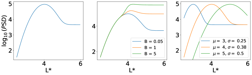
Figure 1: Possible configurations of the initial phase space density distribution function $f$. Combinations shown here are the default initial distribution (a) with $A=9\times 10^{4},B=0.05,\mu=4,\sigma=0.38,\gamma=5$, (b) varied values of $B$ and (c) varied values of $\mu$ and $\sigma$.

IV.1.5 Outer Boundary Condition

The model in Thompson et al. (2020) uses a constant value (Dirichlet) inner boundary to characterise the inner edge of the radiation belt, where particles are lost to the atmosphere. Choices of the outer boundary are less clear. Physically, one expects the PSD to be smooth across the boundary, hence a Neumann (constant gradient/zero flux) boundary may be appropriate. By default, the model uses a constant gradient (Neumann) outer boundary, set at zero, which matches the physics of a slow injection from high-L as represented in our initial condition. However, a Dirichlet boundary allows the modeller to input PSD values, and indeed large-scale models tend to interpolate time-varying outer boundary values from available data. Neither of these methods are designed to use the true edge of the outer radiation belt, which varies considerably when an outer edge is distinct enough to observe at all, Bloch et al. (2021). Since both methods should be physically appropriate for the underlying plasma, in our results we investigate the impact of both choices of outer boundary condition. We will review this outer boundary in the discussion, following our results [S1a].

IV.2 Metric Requirements to Compare Ensemble Members: Time to Monotonicity

Ensemble modelling for predictive purposes use the variability across model runs in the given ensemble, using a given error metric or loss function. We are also interested in examining timescale of radial diffusion, for which we need a quantitative measure.

However, error metrics are not an ideal tool for comparing the evolution of phase space density. They don’t tell us about the evolution of the system state, or properties of that state we are interested in. Therefore one of the secondary goals of this work was to select and investigate potential metrics. Initially, simple error metrics such as mean square error (MSE) were selected. MSE would quantify a scalar difference between distributions, which would be useful for analysis of variation and uncertainty across ensembles. However, the significant variation in scales covered in this problem make it difficult to generalise or compare different cases. We found this regardless of using linear- or log-based scales; thresholds usually would need to be specified for when radial diffusion was “finished enough" or for when two distributions were “similar enough", and the results became dependent on that choice of threshold. Instead, our experiments were analysed with a property that captured the physics of the system we were interested in: time to monotonicity, $t_{m}$. This choice of metric is motivated below. Requirements of the metric used for analysis are [A1]:

• Robustness. The metric used must be insensitive to any thresholds used. It must therefore be scale independent (i.e. work across multiple orders of magnitude, because of Kp dependence)

• Interpretable The metric must aid in understanding the system.

• Radiation belt system specific. The metric must be related to radiation belt modelling; it should provide insight into either the system state, or specific properties related to physical processes.

• Time-series informative. The metric must enable analysis of the evolution of system.

Initially, potential measures were tested, such as the decreasing MSE between distributions at each timestep, the evolution of maximum gradients, the total area and the proportional change in amplitude. All these required an arbitrary threshold to determine when a given experiment was “finished”, the choice of which strongly impacted the time until distributions became similar, particularly for larger Kp. For example, MSE-based metrics varied by orders of magnitude depending on several model choices. No MSE-based metric could be found that worked robustly. Furthermore, many of these metrics ended up being dominated by the inner boundary condition, whereas we wanted to know about the evolution of the entire phase space density distribution.

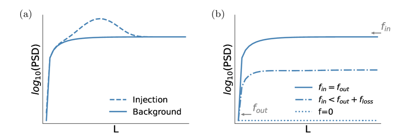
Figure 2: Example phase space density (PSD) distributions. Panel (a) shows the background, “quiet" distribution in solid black lines, which is monotonic, plus a non-monotonic enhancement from local acceleration in dashed lines. Panel (b) shows potential long term (monotonic) PSD profiles: a return to the quiet profile (solid), a similar profile of reduced amplitude after loss from pitch-angle scattering (dot-dashed) and a zero profile (dotted).

To find an appropriate metric of the how the ongoing radial diffusion affected the evolution of the system, we turned to properties of the PSD distribution under radial diffusion. Fig. 2 (a) shows the phase space density profiles we expect on the timescale of radial diffusion. A quiet time, or background distribution, is shown in solid black lines: a low level, high $L$ source of particles feeds the system from constant substorms. Due to the $L$ dependence of the diffusion, the drop-off at low $L$ is quite sharp. In dashed lines, an enhancement of particles due to local acceleration is shown at an intermediate $L$. Following a single enhancement, we expect the distribution to gradually return to a monotonic state via radial diffusion Reeves et al. (2013); Green and Kivelson (2004).

Therefore, since diffusion acts to even out gradients in the PSD, we are more interested in changes in the shape of the PSD distribution, than the total PSD (i.e. the integrated area under the curve). Hence we also include the following criteria:

• Insensitive to total particle population. The metric must be insensitive to shifting the distribution up and down the y-axis.

We chose to work with time to monotonicity, $t_{m}$. When the distribution has become monotonic, the PSD distribution no longer has a peak for radial diffusion to smooth out. $t_{m}$ therefore indicates when the PSD distribution has stopped changing shape; when radial diffusion is no longer changing the properties of the radiation belts. $t_{m}$ is a proxy for whether radial diffusion is still significantly affecting the evolution of the particle distribution. The potential monotonic distributions are shown in Fig. 2 (b); the “background" distribution which is nonzero but unchanging in time (i.e. the influx of particles balanced by constant movement of particles inwards), a shrinking version of this when more particles are lost than enter the domain, and finally a zero profile.

In the results section we use $t_{m}$ to explore how idealised radial diffusion models vary when changing initial settings. $t_{m}$ represents our physical expectations; our intuition that after a localised enhancement the PSD will eventually relax to monotonic distribution. We can test our expectations and how the changing parameters affect these expectations. See Section VI for evaluation of our chosen measure and for alternative approaches.

IV.3 Analytical Approach to Comparing Evolution of Ensemble Members

To study the impacts of varying initial and boundary data, we will utilise tools from he study of deterministic diffusive problems. In particular, we will monitor the number of particles and an energy-like quantity in our simulation domain, defined respectively by the following integrals [A1]:.

$$\mathcal{N} =\int\frac{f}{L^{2}}dL\,,$$ (10)

$$\mathcal{E} =\int\frac{f^{2}}{L^{2}}dL\,.$$ (11)

The former of these ($\mathcal{N}$) is the conventional integral of the distribution function with the appropriate Jacobian for the radial component of the co-ordinate system, due to the use of adiabatic invariant variables. The latter ($\mathcal{E}$) is unconventional in the study of radial diffusion as far as the authors are aware, but is closely related to the $L_{2}$ norm of the distribution function. Such an integral is a linchpin in the study of diffusion in other contexts Strauss (2007). We refer to this integral as an ‘energy’ integral in a loose sense, as it is a positive definite quantity throughout the distribution functions evolution and is minimized precisely when the distribution function’s evolution has ceased (i.e. when $f_{t}=0$). We will investigate how these quantities change in the system and use these changes to confirm or clarify the results from our ensemble runs analysed using $t_{m}$.

In order to understand how these quantities change with evolving $f$ it will be useful to monitor the rate of change of these integrals over time. These rates can be computed explicitly as follows:

$$\mathcal{N}_{t} =\int f_{t}\frac{1}{L^{2}}dL=\int\left(\frac{D_{LL}}{L^{2}}f_{L}\right)_{L}dL=\left[\frac{D_{LL}}{L^{2}}f_{L}\right]^{OB}_{IB}$$ (12)

$$\mathcal{E}_{t} =\int ff_{t}\frac{1}{L^{2}}dL=\int f\left(\frac{D_{LL}}{L^{2}}f_{L}\right)_{L}dL$$

$$=\left[\frac{D_{LL}}{L^{2}}ff_{L}\right]^{OB}_{IB}-\int\frac{D_{LL}}{L^{2}}\left(f_{L}\right)^{2}dL\,,$$ (13)

where $OB,IB$ indicate evaluating the resulting function at the inner and outer boundaries respectively. The rate of change of energy $\mathcal{E}_{t}$ is a useful diagnostic to determine whether the distribution function $f$ is approaching its equilibriated state, as this will be reflected by this rate of change approaching zero. What is clear from the final forms in (Eq. 12) and (Eq. 13) is that the choice of the diffusion coefficient significantly impacts these rates and differing choices may either accelerate or arrest the dynamics as they approach monotonicity. Within this paper, we will restrict ourselves to a specific form of this coefficient, made explicit in the next section, but it is clear that alternative choices may impact the conclusions we draw from this study. Further, these rates are explicitly dependent on the boundary conditions chosen for the simulation as well as the size of the domain. We will return to dependence later when we discuss outcome of the numerical experiments we undertake as the key study of this paper.

As a final comment, the above rates of change generalise quite naturally when loss is included within the radiation belt monitoring. Recall that when loss is included, the radial diffusion equation assumes the form

$$f_{t}=L^{2}\left(\frac{D_{LL}}{L^{2}}f_{L}\right)_{L}-\mathcal{L}f\,.$$

It then follows by repeating the analysis above that the loss-modified rates of change for the number and energy are given by

$$\mathcal{N}_{t}^{loss} =\mathcal{N}_{t}-\int_{IB}^{L_{p}}\mathcal{L}\frac{f}{L^{2}}dL$$

$$=\mathcal{N}_{t}-\int_{IB}^{L_{p}}\frac{1}{\tau(L)}\frac{f}{L^{2}}dL$$

$$\mathcal{E}_{t}^{loss} =\mathcal{E}_{t}-\int_{IB}^{L_{p}}\frac{1}{\tau(L)}\frac{f^{2}}{L^{2}}dL\,.$$

As the new terms are positive definite, the loss effects cause a continual loss of energy as expected, with equilibrium only occurring when $f=0$ for all $L$, or when inward flux from the outer boundary equals the combined loss from the inner boundary and pitch angle scattering. Again, we would also expect particles to move towards lower $L$.

In this section we derive the terms that comprise the changing energy ($\mathcal{E}_{t}$) and mass ($\mathcal{N}_{t}$). The figures comparing these terms, evaluated explicitly for each of our boundary conditions, can be found in Section V where they best support our analysis.

Using our $D_{LL}$ from (Eq. 5), we may decompose the contribution to the rate of change of number and energy respectively in the following way:

$$\mathcal{N}_{t} =\left[D_{0}L^{n-2}f_{L}\right]^{OB}_{IB}$$

$$=-\mathcal{N}_{t}^{(1)}-\mathcal{N}_{t}^{(2)}$$

$$\mathcal{E}_{t} =\left[D_{0}L^{n-2}ff_{L}\right]^{OB}_{IB}-\int D_{0}L^{n-2}\left(f_{L}\right)^{2}dL$$

$$=-\mathcal{E}_{t}^{(1)}-\mathcal{E}_{t}^{(2)}-\mathcal{E}_{t}^{(3)}\,.$$

i.e $\mathcal{N}_{t}$ has two terms and $\mathcal{E}_{t}$ has three. We can now evaluate the role of each term on the distribution function’s evolution, and we start by discussing the effects of the boundary conditions on the number and energy. It is clear that the number of particles in our system can only change based on the boundaries; whether this is a loss or addition will depend on the gradient at each boundary, and the magnitude of that change will be moderated by the location of that boundary owing to the fact that the diffusion coefficient depends on the spatial co-ordinate $L$. The ‘energy’ can not only change due to boundary effects (terms 1 and 2), but also due to an additional term $\mathcal{E}^{(3)}_{t}$ which is dynamical in origin. Terms 1 and 2 depend on the PSD, the gradient of the PSD at that boundary and the location of that boundary. Both of these can contribute to energy increases or decreases in the same way that the number density varies at the boundaries, but the third term informs us on how the energy is minimized due to effects of the distribution function on the interior of our domain. We discuss these effects and their implications for $f$ below.

The third term in $\mathcal{E}_{t}$ is one that will give us insight into how the dynamics of the distribution will evolve to minimise our energy. This term has an integral which depends on the square of the derivative in $L$. As this is a non-negative quantity, this ensures that the integral contributes to energy loss (as it is preceded by a negative sign) whilst gradients in the distribution function exists, up to a point where the contributions from the boundary conditions balance this out. This is an property identical to Cahn-Hilliard diffusive dynamics, where diffusive terms correspond to energetics that penalise the formation of (sharp) gradients Kendon et al. (2001); Stratford et al. (2005). This penalty is enhanced for gradients occurring at higher values of $L$, as their contribution to the integral will be increased by a positive power of $L$, suggesting that the distribution function can minimise this integral by moving gradients to lower values of $L$. Thus, $\mathcal{E}_{t}$ decreases towards a long-term solution through diffusion to reduce gradients $(f_{L})^{2}$ and through the population moving towards lower $L$, and this movement of the population will be increased for higher powers $n$.

V Results

Our methodology was to begin with $t_{m}$, to find out how long it takes a given initial distribution to reach a monotonic state, and how this varies with initial conditions. We first compared $t_{m}$ with Kp for each parameter in Eq. 9. For $t_{m}$ we note that from Eq. 2, we expect timescale to vary significantly with Kp. Kp is a proxy for strength of radial diffusion, even though $Kp>6$ is unlikely. Since we expect time to monotonicity to depend on Kp we primarily use a heatmap for the ensemble used to investigate each parameter, demonstrating how $t_{m}$ varies with each (Kp, parameter) pair. To aid understanding, these results are also presented in an alternate format, where the $t_{m}$ for each Kp are plotted as a line. Each experiment ran for a week; model runs where monotonicity were not reached are left empty.

Following our initial $t_{m}$ analysis, we then investigated any noteworthy results, for example by looking at the evolution of the phase space density of a specific simulation. In general, runs with a Neumann outer boundary condition (zero flux) are shown on the left, while the right hand column corresponds to a Dirichlet outer boundary condition (constant value)

Finally, we incorporated our analysis from Section IV.3 for each parameter to understand and generalise any patterns we saw. Our $\mathcal{N,E}$ experiments are also run for a week, using $n=6$ in our diffusion coefficient. Just as for our $t_{m}$ analysis, we calculated $\mathcal{N,E}$ for each returned timestep (every six hours).

V.1 Results Part 1: Without loss rate

Each parameter in the initial condition was systematically investigated. Selected results are presented in the main text in an order chosen to best convey our conclusions; the full set of individual $t_{m},\mathcal{N}$ and $\mathcal{E}$ experimental figures can be consulted in the supplementary material, labelled as Figure SX.

V.1.1 The difference between the two outer boundary conditions

Overall, it is clear from Figure S1 that generally, more runs with a Neumann (fixed gradient) outer boundary reach a monotonic state within a week. We will investigate the two outer boundary conditions before examining the effect of each parameter in the initial condition. To understand the evolution of $f$ in these experiments, in Fig. 3 we show the phase space density for both Neumann and Dirichlet outer boundary conditions, with an outer boundary located at $L_{outer}=6.5$. We use default settings for the initial PSD, a Kp of 4 and run for a week. Panels (a) and (b) show the heatmap, while waterfall plots are in panels (c) and (d).

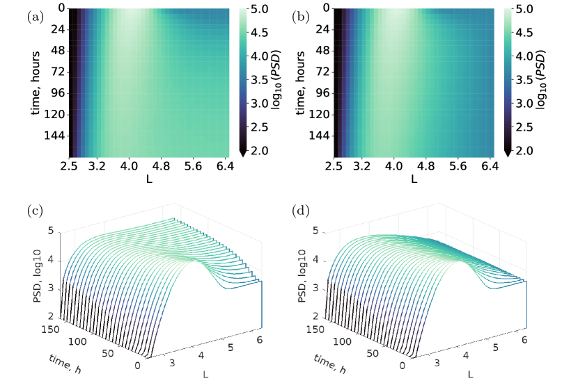
Figure 3: Phase space density over a week, with Neumann (constant gradient, left) and Dirichlet (constant value, right) outer boundaries.

In both experiments the peak remains high and moves inwards. However, there is a difference in the outer part of the simulation. The plateau becomes significant for the Neumann boundary but not for the Dirichlet boundary. This makes sense as the outer boundary value is able to rise for the Neumann case, reflecting outward radial diffusion. For Dirichlet runs the outer boundary value cannot rise, but particles can be lost. Note that the amplitude of the Neumann peak is still comparable to the Dirichlet case (4.55 and 4.52 $\log_{10}(PSD)$ at $L=3.9$ and $3.7$ respectively); it is the plateau that has changed. More Neumann experiments reach monotonicity as the plateau can rise instead of having to wait until the peak diffuses completely inwards. This inability for the high-$L$ (to the right of the peak) PSD to reach (positive) monotonicity independently of the left part is one reason why it takes longer for the Dirichlet runs to reach monotonicity. This corresponds to outward radial diffusion varying depending on the outer boundary condition [S1b].

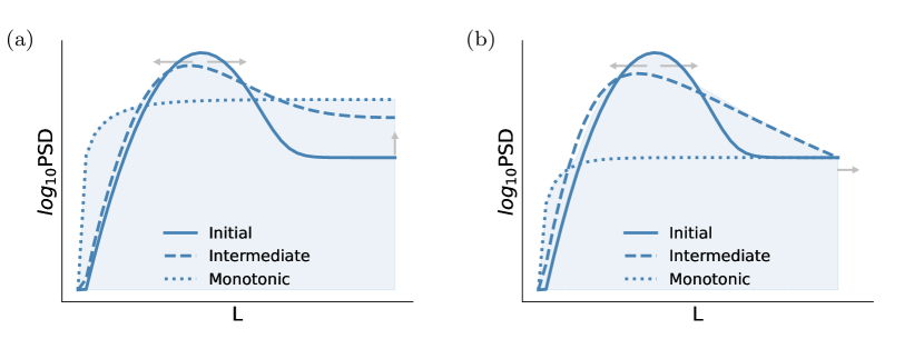
Figure 4: How phase space density profiles with Neumann and Dirichlet outer boundary conditions reach a monotonic state.(Left) Neumann runs reach monotonicity by the high-$L$ population increasing. The Dirichlet runs (right) reach monotonicity by material leaving the domain until the peak has diffused away. The point at which each reach monotonicity is very different (see monotonic states in dotted blue, and intermediate states in dashed blue.)

For a more realistic outer boundary condition we need to consider these, along with the fact that we don’t currently have a clear outer boundary location. We discuss all these factors together in Section VI.4.

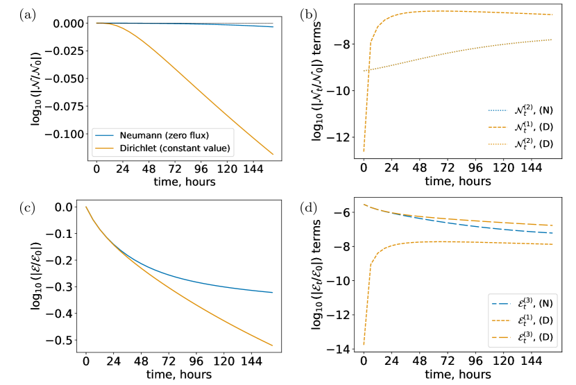
Figure 5: The value of our mass-like quantity, $\mathcal{N}$ and our energy density-like quantity, $\mathcal{E}$, across a week for both Neumann (blue) and Dirichlet (orange) outer boundary conditions. (a) shows how $\mathcal{N}$ evolves across the week; (b) shows how loss from the outer and inner boundaries contribute to a reduction in $\mathcal{N}$ ($\mathcal{N}_{t}^{(1)}$ and $\mathcal{N}_{t}^{(2)}$ respectively); (c) shows how $\mathcal{E}$ evolves across the week; (d) shows how loss from outer and inner boundaries and from the reconfiguration contribution to the reduction in $\mathcal{E}$ ($\mathcal{E}_{t}^{(1)},\mathcal{E}^{(2)}_{t}$ and $\mathcal{E}_{t}^{(3)}$ respectively). (a) and (b) are both normalised by $\mathcal{N}$ at time $t=0$ and (c) and (d) are normalised by $\mathcal{E}$ at time $t=0$.

We can also examine how the evolution of our mass- and energy-like densities varies with Neumann and Dirichlet outer boundary conditions. Fig. 5 shows $\mathcal{N,E}$ across the week, plus the components of $\mathcal{N}_{t},\mathcal{E}_{t}$. Panels (b) and (d) show the absolute value of components on a log scale to make order of magnitude comparisons earlier; in rare cases in later analyses where the change becomes positive (i.e. a gain in mass or energy, rather than a loss), this is specified.

By definition, for Neumann experiments $\mathcal{N}_{t}^{(1)}=0$, i.e. mass is only lost through the inner boundary. For the Dirichlet experiments it is clear that the outer boundary dominates loss, with $\mathcal{N}^{(1)}_{t}$ up to two orders of magnitude larger than $\mathcal{N}^{(2)}_{t}$, hence the number of particles decreases more rapidly. We find that less than 0.8% of the original mass is lost with a Neumann outer boundary, while around 24% of the mass is lost with a Dirichlet boundary [S1b].

Comparing the individual terms contributing to changes in mass, we see that loss from the inner boundary is the same across the week regardless of the outer boundary (and therefore independent of the different interior distribution as the system evolves). For inner boundary loss to be big enough to vary, one must run experiments with very large diffusion coefficients (e.g. using $Kp=9$ in Eq. 2) or for a much longer time.

The results for our $L_{2}$ norm $\mathcal{E}$ are somewhat counterintuitive. In total we know that experiments with a Neumann outer boundary can eventually reach a lower-$\mathcal{E}$ state (zero everywhere) than experiments with a fixed outer boundary value, where the minimum-energy state will have the same fixed value at $f|_{OB}$ as the initial condition. However, we find that Neumann simulations appear to be reaching a limiting state, where $\mathcal{E}_{t}$ is increasingly smaller and $\mathcal{E}$ relatively unchanged.

For a Neumann outer boundary, $\mathcal{E}_{t}=-\mathcal{E}_{t}^{(3)}$. While the Dirichlet outer boundary can contribute to changing energy ($\mathcal{E}_{t}=-\mathcal{E}_{t}^{(1)}-\mathcal{E}_{t}^{(3)}$ ) we can see from Fig. 5(d) that the dominant mechanism for energy loss is mostly from the reconfiguration term $\mathcal{E}^{(3)}$. However, this term accounts for more energy loss when the outer boundary is Dirichlet rather than Neumann, because there are more steeper gradients when the outer boundary is fixed. Since $\mathcal{E}_{t}$ depends on gradients ($f_{L}$), $\mathcal{E}_{t}$ is larger for Dirichlet runs as there are gradients both sides of the peak, rahter than just to a plateau. For Neumann experiments, the gradients rapidly flatten into a plateau at higher $L$. Remember that our equation for $\mathcal{E}$ has a factor of $\frac{1}{L^{2}}$ in it: the same PSD at a higher $L$ contributes less to the norm, because it can be moved around more easily. Hence Neumann runs have a lower $\mathcal{E}_{t}^{(3)}$. Once the plateau has been reached, the only way to lose energy is for material to move down the gradient (and then out through the inner boundary). This process is slow and so $\mathcal{E}$ is effectively limited. On the other hand, the Dirichlet experiments are more effectively moving material to higher $L$, and then out of the domain. Having an outer boundary that allows flux in/out means that $L_{2}$ norm is reducing more quickly than when we allow the PSD at the outer boundary to change. Hence Neumann appears to be reaching a limiting state first, where $\mathcal{E}_{t}=0$ and $\mathcal{E}$ is unchanging, even though we know that if left forever, it can reach a lower-energy state than Dirichlet [S1b;S1e].

V.1.2 Significant properties of the initial condition ($\mu,B$)

The results of systematically investigating each parameter, using first time to monotonicity $t_{m}$ and then our quantities $\mathcal{N,E,N}_{t},\mathcal{E}_{t}$, are shown here. Those properties we have considered to have a significant impact on time to monotonicity are presented in detail, whilst remaining properties are covered briefly in Section V.1.3 [P1b;S3a].

Step size $B$: The step size $B$ corresponds to a system where the phase space density is higher further out in the radiation belts; i.e. a situation where inwards radial diffusion from a distant source has already occurred. A higher step therefore corresponds to radiation belts that have more material before the enhancement occurs.

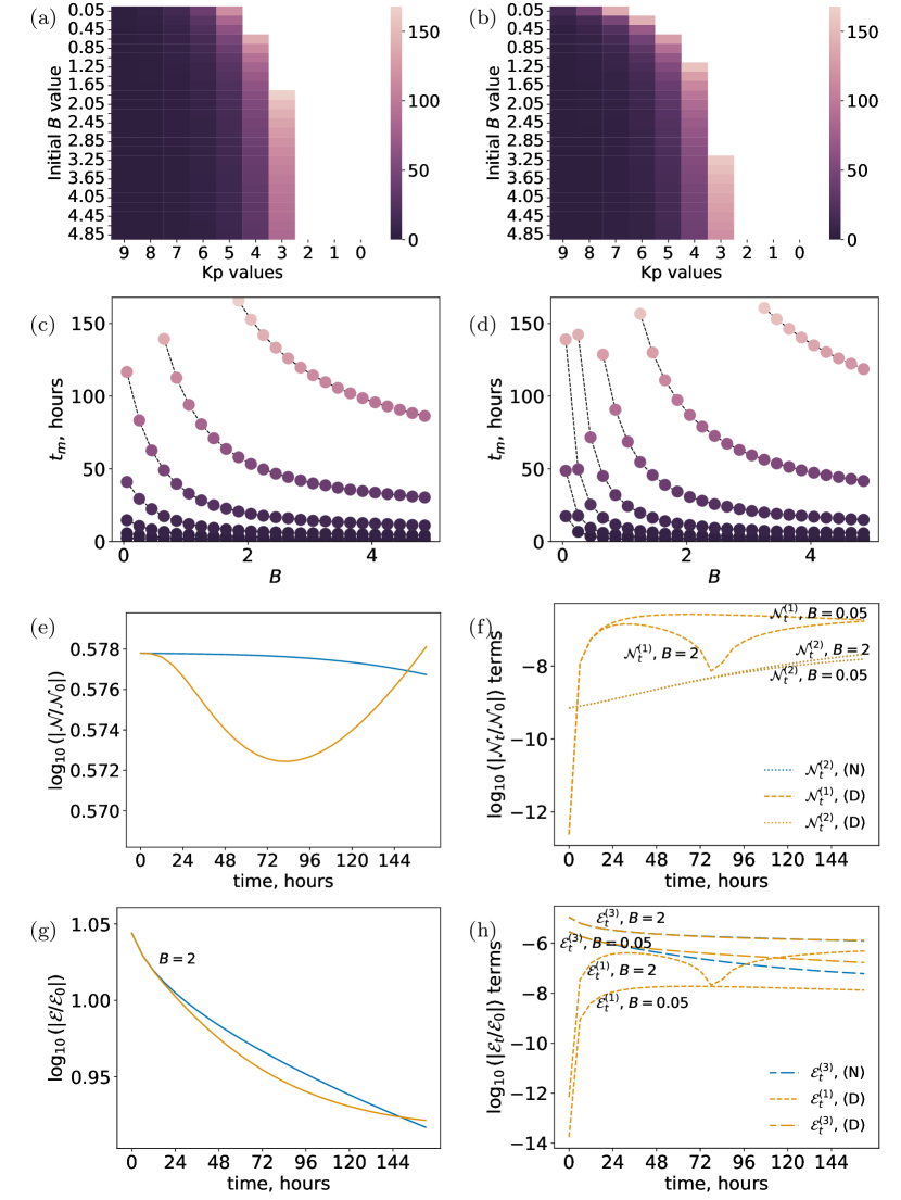
Figure 6: Selected results for the impact of increase in step size $B$ on the evolution of the system under radial diffusion. Left: Neumann. Right: Dirichlet. The top two rows show the change in time to monotonicity $t_{m}$ with $B$, whilst the bottom panels show the changing mass-like and energy-like quantities $\mathcal{N}$ and $\mathcal{E}$. $\mathcal{N,E}$ and $\mathcal{N}_{t}^{(1,2)},\mathcal{E}_{t}^{(1,2,3)}$ are normalised by the initial values of $\mathcal{N}$ and $\mathcal{E}$ respectively. All $\mathcal{N}_{t},\mathcal{E}_{t}$ terms are shown as absolute values to enable a log scale.

Fig. 6 (a) and (b) show how time to monotonicity $t_{m}$ varies with both Kp and increasing step size. When starting with a larger step size, we find that monotonicity is reached sooner for both outer boundary conditions. This behaviour is as expected as with an increased $B$, $f$ is already closer to a monotonic state. Again, more ensemble runs with Neumann outer boundary reach monotonicity. Looking at this information in the alternative format in panels (c) and (d), we see that for both outer boundary conditions, $t_{m}$ appears to increase exponentially for smaller step sizes.

Our $\mathcal{N,E}$ results show that the evolution is not necessarily straightforward, however. Fig. 6 (e) shows the total mass in $f$ across the week simulated, for the larger step size $B=2$ for both Neumann and Dirichlet outer boundary conditions (the comparison against the default value can be found in Figures S3 and S4). As expected, the total number of particles changes very little for a zero flux (Neumann) outer boundary. However, when the overall mass response when mass can flow across the outer boundary (Dirichlet experiments) we see that for a larger step size $B=2$, the experiment starts to gain mass at around 80 hours. From the mass change terms $\mathcal{N}_{t}$ in Fig. 6(f) this is clearly from the outer boundary, when the distribution drops below the fixed outer boundary point $f|_{OB}$. At this point the gradient $f_{L}|_{OB}$ will be positive, and material will flow into the domain. (The plain $\mathcal{N}_{t},\mathcal{E}_{t}$ components can be found in the supplementary materials for confirmation that this becomes positive, rather than the absolute log values shown here). Inner boundary loss varies with $B$ but but is again independent of the outer boundary condition.

The $L_{2}$ norm $\mathcal{E}$ is much higher for a larger step, and the norm reduces over several orders of magnitude (see Fig. 6(g)). The Dirichlet run started out losing more energy than Neumann (as we also see using default settings above) but later in the week, energy loss drops off and the Neumann case has lower energy (and is therefore closer to a point where the dynamics have stopped changing). This is because there is an increase in the norm ($\mathcal{E}$) with the reversed outer boundary flow; however, the corresponding energy change term $\mathcal{E}_{t}^{(1)}$ reaches a comparable magnitude to the dominant reconfiguration term $\mathcal{E}^{(3)}_{t}$. Therefore the total change $\mathcal{E}_{t}$ for the Dirichlet case with $B=2$ becomes very small, while the Neumann case is still reducing in norm because the PSD can be reconfigured (diffused).

Physically, this means that with a higher step, we are finding that the Neumann case reaches a lower energy state by the end of the week than the Dirichlet experiment, unlike our default settings Fig. 5. For the Dirichlet case, the constant outer boundary value is higher than the peak, allowing material to come in through the outer boundary. This experiment is in a state where the main dynamic is a constant churn of mass coming in and then being diffused to lower $L$ to reduce the entire distribution to a lower energy state. Physically, this corresponds to an infinite source at the outer boundary if we were to run this indefinitely. See Section VI for our overall conclusions on more suitable outer boundary settings.

Enhancement location $\mu$: The Gaussian in the first term of Eq. 9 corresponds to an enhancement, and $\mu$ corresponds to the location of this enhancement in $L$.

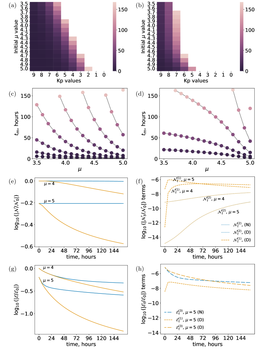
Figure 7: Selected results for the impact of increase in enhancement location $\mu$ on the evolution of the system under radial diffusion. As in Fig. 6, the top two rows pertain to time to monotonicity $t_{m}$ and the bottom two to the mass-like quantity $\mathcal{N}$ and the $L_{2}$ norm $\mathcal{E}$. Neumann and Dirichlet outer boundary conditions are shown in the left and right columns respectively.

Considering $t_{m}$ across a variety of enhancement locations in Fig. 7, we find that monotonicity is reached more quickly for higher $\mu$ for both outer boundary conditions, although the shape of the dependence is seen to be very different in Fig. 7(c) and (d). A sooner $t_{m}$ for higher $\mu$ makes sense as $D_{LL}$ will be larger at higher $L$, so when the peak is located at higher $L$, diffusion to flatten this peak happens more quickly. Again, far more runs reach monotonicity with a Neumann outer boundary.

Fig. 7(a) and (b) show us the general relationship between each parameter and $t_{m}$, while (c) and (d) show us the specifics of each relationship. We see that the relationships between $\mu$ and $t_{m}$ for each Kp are quite different for the different outer boundary conditions. This disparity could be due to the different mechanism to the right of the enhancement; a zero flux outer boundary condition allows the plateau to rise and reach monotonicity to the right of the peak, while the same region with a constant value outer boundary cannot reach monotonicity until the enhancement has completely diffused, although material can be lost through the boundary.

The bottom two rows of Fig. 7 compare the evolution of $\mathcal{N,E}$ across the simulation for the default value of $\mu=4$ to a more distant peak at $\mu=5$. The total number of particles $\mathcal{N}$ is higher when $\mu$ is lower, which is as expected since the step extends further inwards. There is little change in mass with $\mu$ for Neumann runs, also as expected. There appears to be different amounts of mass lost in Dirichlet simulations, so we consider the outer and inner boundary particles losses $\mathcal{N}_{t}^{(1)}$ and $\mathcal{N}_{t}^{(2)}$ in (f). These are always negative (particles are only lost, not gained) but look quite different. The outer boundary loss dominates for both values of $\mu$. With a higher-L enhancement, the inner boundary loss is less. Therefore whilst the outer boundary loss is comparable, the higher the $\mu$, the more strongly that outer boundary loss dominates over the loss from the inner boundary. Fig. 7 (g) shows the evolution of $\mathcal{E}$. Lower values of $\mu$ (enhancements at lower $L$) actually result in higher $L_{2}$ norms, because you have more PSD total (for the same reason as the mass above) and more of this mass is at lower $L$. In both cases the Neumann experiments reach a configuration where $\mathcal{E}_{t}$ is very small and $\mathcal{E}$ stops changing. The Dirichlet experiment with a higher-L enhancement rapidly loses $\mathcal{E}$ but by the end of the week, is no longer changing much. In (h) we can see the terms of $\mathcal{E}_{t}$ for each experiment. For readibility, we show only the $\mathcal{E}_{t}$ terms for $\mu=5$ here. The reconfiguration energy loss ($\mathcal{E}_{t}^{(3)}$) evens out more quickly for Neumann experiment with $\mu=5$ than with the standard initial condition, presumably because it is easier for the step to rise up and plateau in a monotonic state. For the Dirichlet experiment the reconfiguration term $\mathcal{E}_{t}^{(3)}$ dominates, but rapidly drops off until it is comparable with energy loss at the outer boundary.

We find that an initial distribution with more material at high $L$ (i.e. step size $B$) and with an enhancement at high $L$ (i.e. $\mu$) diffuse more quickly. $B$ and $\mu$ are the most significant initial conditions, yet the specific evolution of the system varies depending on interaction with boundary conditions [P1b].

V.1.3 Minor properties of the initial condition ($A,\sigma$)

Amplitude $A$: We do not expect the amplitude of the initial condition to impact our time to monotonicity. This is because the radial diffusion equation is linear and so amplitude scalings can be factored out. Indeed, setting $f=Ag(L,\mu,\sigma,t)$ one finds that

$$f_{t}=L^{2}\left(\frac{D_{LL}}{L^{2}}f_{L}\right)_{L}\qquad\Rightarrow\qquad g_{t}=L^{2}\left(\frac{D_{LL}}{L^{2}}\cdot g_{L}\right)_{L}\,,$$

which will have the same solutions as Eq. 1, which are independent of $A$. As monotonicity is a property of a given solution, the time to reach this monotonic solution is independent of $A$. This is verified in the supplementary materials (Figure S1 (a), (b)) where we observe that time to monotonicity varies with $Kp$ as expected and does not vary with initial amplitude. We note that although the energetic quantities $\mathcal{N,E}$ scale with $A$ and $A^{2}$ respectively, they evolve on the same timescales as Fig. 5 via similar arguments to the above.

Enhancement width $\sigma$: Fig. 8 (a) and (b) show that for both Neumann and Dirichlet boundaries, $t_{m}$ is reached more quickly for narrower peaks; i.e. for smaller values of $\sigma$. This difference is only slight. There are two aspects at work here; a wider $\sigma$ will have access to larger diffusion rates at high $L$, but the gradient $f_{L}$ will be less steep. We can examine these components using $\mathcal{N}$ and $\mathcal{E}$ to determine which is more significant.

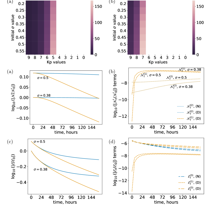
Figure 8: (Top row) time to monotonicity $t_{m}$ for enhancement width $\sigma$ vs Kp over a week, for Neumann (a) and Dirichlet (b). (Middle row) The mass-like quantity $\mathcal{N}$ for $\sigma=0.38$ and $0.5$, and the components of the time derivative $\mathcal{N}_{t}$. (Bottom row) Same as the middle row, but for the $L_{2}$ norm $\mathcal{E}$.

An enhancement across more $L$ has somewhat more mass and appears to loss mass more quickly for both Neumann and Dirichlet outer boundary conditions. Despite the fact that experiments with a larger $\sigma$ also start with higher $\mathcal{N}$, at the end of the week, 98% and 75% of the mass remains from the initial population (for Neumann and Dirichlet experiments respectively), compared to 99% and 76% remaining from our default experiments. Both experiments with a wider enhancement lose more from the inner boundary (Fig. 8(d)), again showing that the initial condition controls more loss from the inner boundary than changes in the outer boundary condition. Loss from the outer boundary is slightly more with a larger $\sigma$, but is roughly comparable.

Total $\mathcal{E}$ is higher for a larger $\sigma$, which makes sense as the experiment has more mass and hence larger $\int f^{2}dL$; the distribution $f$ is further from a steady state. All $\mathcal{E}_{t}^{(1,3)}$ with $\sigma=0.5$ are slightly larger, but overall very similar. Unsurprisingly, with similar $\mathcal{E}_{t}$ but a larger starting $\mathcal{E}$, experiments starting with a larger $\sigma$ end up retaining proportionally more of the initial energy (37% and 58% for Dirichlet and Neumann respectively, rather than 30% and 47% of the initial energy when using default $\sigma$). Overall, with a wider $\sigma$, the Dirichlet experiment loses more $\mathcal{E}$, even though $t_{m}$ is slower. The results from the investigation of $\sigma$ indicate that the trade-off between gradient in the PSD and the $L$-dependence of $D_{LL}$ is subtle and nuanced (a wider enhancement has a less steep gradient but samples higher $D_{LL}$).

V.1.4 Gradients versus the $L$-dependence of $D_{LL}$

The $\sigma$ results suggest we should compare the role of the spatial (i.e., $L$) dependence and the gradients in the distribution function on the overall amount of diffusion. We consider their role in reconfiguration term $\mathcal{E}^{(3)}_{t}$, since this generally dominates $\mathcal{E}_{t}$. With a constant diffusion coefficient, only the gradient term would contribute to the $\mathcal{E}^{(3)}$. With an $L$-dependent $D_{LL}=D_{0}L^{n}$, both $(f_{L})^{2}$ and $D_{0}L^{n-2}$ will contribute to $\mathcal{E}^{(3)}$. We simply compare the order of magnitude of these components via a ratio, shown in Fig. 9. Overwhelmingly, it is the gradient component $(f_{L})^{2}$ that dominates. This is unsurprising once one considers that $D_{0}\sim 10^{-10}$ s^-1.

Throughout this analysis we have found that one must consider the whole domain; for example, the amount of diffusion is not limited by the smallest $D_{LL}$ but also the shape of the distribution, loss, the choice of domain etc. This is because $\mathcal{E}^{(3)}$ is the dominant component of $\mathcal{E}_{t}$, which determines the PSD evolution. And $\mathcal{E}^{(3)}$ is an integral over the entire simulation domain.

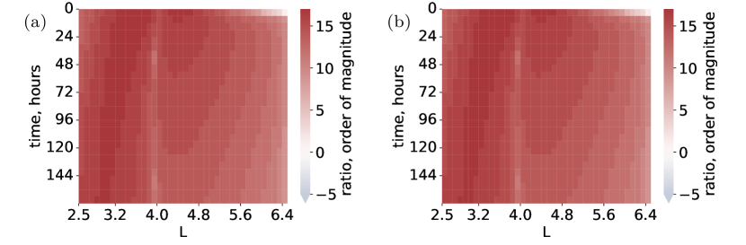
Figure 9: What contributes most to the reconfiguration term $\mathcal{E}_{t}^{(3)}$ (which dominates the evolution of the system)? We compare the two terms $(f_{L})^{2}$ and $D_{0}L^{n-2}$, for $n=6$. (a) is Neumann, (b) is Dirichlet

Fig. 9 shows the order of magnitude of the ratio of $(f_{L})^{2}$ to $D_{0}L^{n-2}$ for $n=6$. Over the whole domain, the gradients clearly have more impact than the L-dependence of the diffusion coefficient. However, with a longer domain, this will begin to change, particularly for a Neumann (zero flux) outer boundary, where there are fewer gradients. Using an idealised $D_{LL}$, gradients almost always dominate over the effect of $D_{LL}$ increasing with $L$. This will by why wider enhancements (larger $\sigma$) take longer to reach monotonicity when using our operational (Ozeke) $D_{LL}$: there are consequently shallower gradients [S1e].

We find that the PSD gradient $f_{L}$ contributes more to the evolution of the system than the diffusion coefficient $D_{LL}=D_{0}L^{6}$ [A2].

V.1.5 Outer edge of domain, $L_{outer}$

In this experiment we varied the domain for the simulation to see what difference it made. A Dirichlet (fixed value) condition is used in the majority of operational radiation belt models, to reflect observations. The simulation domain is curtailed to the location of the spacecraft; different $L_{outer}$ values then correspond to using data from different spacecraft missions to set this outer boundary. Both types of outer boundary condition are investigated in this phase of experiments and the Dirichlet experiments retain the outer boundary value fixed in the initial condition.

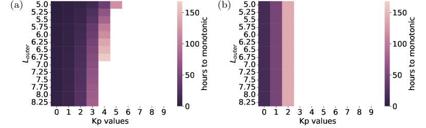
Figure 10: Time to monotonicity $t_{m}$ for $L_{outer}$ vs Kp over a week, for Neumann (left) and Dirichlet (right) outer boundary conditions.

For a Neumann outer boundary condition, a more distant outer boundary (larger $L_{outer}$) took longer to reach monotonicity; i.e a smaller domain reached monotonicity more quickly (Fig. 10(a)). This suggests that the choice of outer boundary location changes the shape of the PSD distribution. For Dirichlet conditions, $t_{m}$ was independent of domain size.

To investigate this, we compare two Neumann runs where we vary the outer boundary location to be $L_{outer}=6.5$ and $7.5$. (Equivalent plots for Dirichlet can be found in the supplementary materials. Fig. 11 shows the PSD distribution at eight equally distant times throughout the week, with Kp=4 and using Ozeke $D_{LL}$.

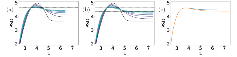
Figure 11: (a) Eight phase space density distribution snapshots from a week long simulation, with a Neumann (zero gradient) boundary at $L=6.5$. (b) Eight snapshots with the boundary at $L=7.5$. (c) The final distribution for each of those.

The distance between peak, and plateau edge (both indicated with dotted lines) by the end of the week is much larger for the run with a wider domain, in Fig. 11(b). The effect of this can be seen more clearly by considering the PSD at the final timestep, in Fig. 11(c). The run with $L_{outer}=6.5$ is more close to monotonic because the value of the outer boundary has raised higher. Despite the larger $D_{LL}$ at high $L$, more reconfiguration of the distribution is needed for a longer domain governed by the same equation - and as was seen in Section V.1.4, the gradients are still more important than the $D_{LL}$ up to $L=6.5$. Although the material in the peak being diffused outwards can be spread across more $L$ when there is a more distant $L_{outer}$, and large $D_{LL}$ values at high $L$ encourage this, the material has to travel farther before the plateau rises and monotonicity is reached. The Neumann $t_{m}$ dependence on domain (i.e. on $L_{outer}$ arises because the shape of the distribution varies with changes in the simulation domain.

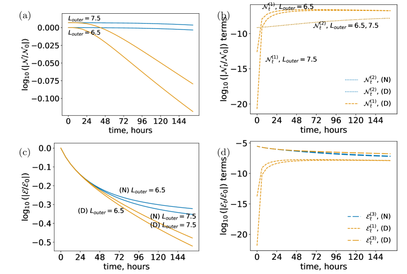
Figure 12: The changing mass-like and energy-like quantities $\mathcal{N}$ and $\mathcal{E}$ when the outer boundary location and condition are varied. The default $L_{outer}=6.5$ is compared to $L_{outer}=7.5$. The top row shows the total $\mathcal{N}$ and the components of the time derivative $\mathcal{N}_{t}$. The bottom row shows the same for the $L_{2}$ norm $\mathcal{E}$.

Analysis of $\mathcal{N}$ in Fig. 12 (b) indicates that neither the outer boundary location or condition affects loss from the inner boundary. For Dirichlet experiments with varying $L_{outer}$, mass loss from the outer boundary is of comparable order within a few hours, regardless of where that outer boundary is. This corroborates findings in Section V.1.4 that the gradients in the PSD distribution dominate diffusion over the entire domain, rather than higher diffusion coefficients located in one region. While the extra mass at time $t=0$ was obvious for a longer domain, the change in initial $\mathcal{E}$ is negligible, as can be seen in Fig. 12(c). However, the evolution of the $L_{2}$ norm is nuanced; despite having $\mathcal{E}_{t}$ terms of similar order (Fig. 12(d)), with a longer domain, the Neumann experiments reaches a lower level of $\mathcal{E}$, while the Dirichlet experiment has a greater value of $\mathcal{E}$.

The mechanism behind these results are, unsurprisingly, the rising plateau for Neumann and the outer boundary flux for Dirichlet experiments. In order for Neumann experiments to reach a configuration of lower $\mathcal{E}$, the high-$L$ plateau rises. With a longer domain, this means that there are more particles at high $L$, hence $\mathcal{E}$ can be lower than with the same number of particles at a lower $L$. Additionally, $\mathcal{E}^{(3)}$ is slightly larger for $L_{outer}=7.5$ than $6.5$, which can be attributed to outward radial diffusion due to the longer domain and higher $D_{LL}$ at $L=7.5$. For the Dirichlet case, the reconfiguration energy change is almost exactly the same. However, more is lost to the outer boundary for $L_{outer}=7.5$ than $6.5$. Even though they lose roughly the same each hour after 70 hours, this is enough to make $\mathcal{E}$ slightly lower for $L_{outer}=6.5$

Using $\mathcal{N,E}$, we find that the choice of outer boundary location changes the shape of the PSD distribution for Neumann; in exactly the same manner, $t_{m}$ varies depending on the outer boundary location. For different outer boundary conditions, a different outer boundary location could result in heading faster or slower to a state where the dynamics are minimally changing (i.e. to minimum $\mathcal{E}$). In Section VI we discuss outer boundary choices, including the applicability of using a Dirichlet outer boundary that is fixed, but not using observations [P1c].

V.2 Results Part 2: Including loss rate

Loss from pitch angle scattering is significant and should be included to see how it relates to the timescale of radial diffusion. We include this loss by modelling the electron lifetime.

V.2.1 The difference between the two outer boundary conditions, with loss

In general, with loss it is no longer always true that more Neumann experiments reach monotonicity; nevertheless, they still have shorter $t_{m}$ than Dirichlet experiments. All the $t_{m}$ plots can be found in supplementary materials; again we select the results that inform us about the overall pattern.

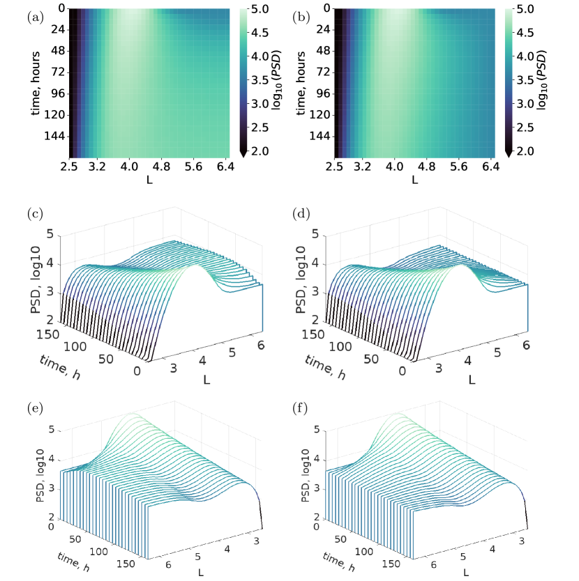
Figure 13: Left: Neumann. Right: Dirichlet. Row 1: Heatmaps of log₁₀PSD. Row 2: waterfall plots (same as Fig. 3). Row 3: waterfall plots from the back.

Fig. 13 show experiments with pitch angle loss for the default initial condition. Neumann and Dirichlet runs look very similar, suggesting that pitch angle loss may control more of the dynamics than the outer boundary condition. The analytic quantities $\mathcal{N,E}$ for these runs confirms this;

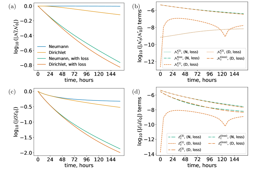
Figure 14: Same as Fig. 5 showing the difference between Neumann and Dirichlet experiments but with additional experiments containing loss from pitch angle scattering. The second column (b) and (d) showing mass and energy moment change terms only the terms for the loss experiments for readibility; full versions can be found in the supplementary materials.

loss from the pitch angle scattering approximation dominates over loss from the outer or inner boundary Fig. 14(b), and the evolution of $\mathcal{E}$ with loss looks similar regardless of outer boundary condition, unlike the runs without loss (Fig. 14(a)). The experiments including pitch angle loss are heading much more quickly towards a steady state, and after around a hundred hours the experiments are not changing much in $\mathcal{E}$, as $\mathcal{E}_{t}\sim 0$.

$t_{m}$ is more complex to analyse. Over the span of the week, enough mass is lost that the Dirichlet run begins to gain mass. Just as without loss, particles entering the domain are contributing to an increase in $\mathcal{E}$ which results in a final $\mathcal{E}$ that is higher for Dirichlet than Neumann. As a result, the Neumann case is closer to a steady state. Loss from pitch angle scattering effectively mimics the reduction in PSD that would occur over a very long timescale of radial diffusion, as it is strongest near the edge of the plasmapause (which is located around the bulk of the enhancement). With a constant inflow of particles, Dirichlet runs have a higher $\mathcal{E}$ but do not come closer to monotonicity. Electron lifetime loss is creating a new local minimum in the PSD, and so the distribution is not monotonic. To demonstrate what is happening in Fig. 14 for both Neumann and Dirichlet runs, the diagram in Fig. 15(a) shows an example phase space density distribution with this additional minimum. This physical profile is corroborated by the fact that $\mathcal{E}_{t}^{loss}>\mathcal{E}_{t}^{(3)}$ and therefore loss dominates over reconfiguration in the systel evolution. We will expand on the consequences of this below. Finally, there is a difference in inner boundary flux; all experiments including lifetime loss have the same, lower flux [S1b;S4].

V.2.2 When $t_{m}$ can never be reached: how $\mathcal{L}$ affects monotonicity

Although experiments with loss $\mathcal{L}$ that reach monotonicity do so quicker than they did without $\mathcal{L}$, for all parameters there are several initial values that reached monotonicity without loss but no longer do once loss is included, usually at lower Kp (i.e. weaker radial diffusion relative to the same loss). The reverse is rarely true; only for narrow $\sigma$ and $L_{outer}=5.0$ is a $t_{m}$ found with $\mathcal{L}$ where none was found before. In this section we explain the physical mechanism behind this general pattern; again, all individual $t_{m}$ plots can be found in the supplementary materials, Figure S5.

The existence of experimental setups that will never reach monotonicity is most clearly demonstrated by following a case where $L_{p}>\mu$ (Fig. 15)(b). There will be loss everywhere left of $L_{p}$. In the region $<\mu<L<L_{p}$, if loss $\mathcal{L}$ is strong enough it can work against monotonicity by creating a minima. The second row of Fig. 15 demonstrates how this case can evolve for Neumann and Dirichlet outer boundary conditions, using default initial conditions, the same loss with the default plasmapause at $Lp=5$ and $Kp=4$ in the diffusion coefficients. The Neumann and Dirichlet (Fig. 15(c) and (d) respectively) experiments show that even when the distribution is much reduced (over 24 and 72 hours respectively), it is not monotonic. (Note that where the loss does not dominate over radial diffusion, then instead the effect of the loss is for the overall distribution to reduce more quickly, but still maintain the characteristic diffusion distribution (e.g. the intermediate distribution in Fig. 2(b)))[S3a;S3b]

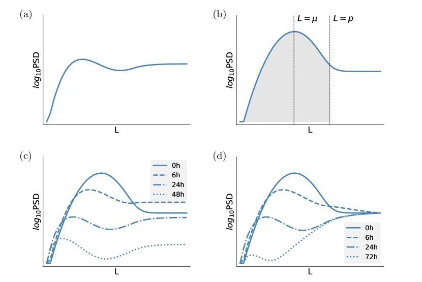
Figure 15: (a) shows a PSD with an enhancement, where pitch angle scattering at higher $L$ than the enhancement has resulted in a new minima. (b) shows the case where this occurs; when the plasmapause is at higher $L$ than the enhancement ($Lp>\mu$) then the loss region (shaded) includes the area to the right of the enhancement, which can prevent reaching monotonicity. The second row shows how the PSD distribution evolves when loss dominates over the diffusion; the distribution may never reach monotonicity but will look different for Neumann (left) and Dirichlet (right) outer boundary conditions. The second row is from experiments with the default initial condition, $Kp=4$ and $Lp=5$.

V.2.3 Loss affects the evolution of diffusion more than most properties of the initial condition

In general, initial conditions impact the diffusion in a similar manner to without loss, for example $t_{m}$ varies significantly with $\mu,B$. In this section, variation of each parameter is compared to the case without loss. Again, we select the most significant results here, while all the figures can be found in the supplementary materials. Note that each $\mathcal{N,E}$ is normalised using the initial $\mathcal{N}_{0},\mathcal{E}_{0}$ for the high-parameter experiment without loss, whereas in Section V.1 they were normalised against the initial values $\mathcal{N}_{0},\mathcal{E}_{0}$ for the phase space density using all default parameter values. This normalisation was chosen to ensure that the effect of each parameter is extracted, rather than including more of the generic evolution with loss which was explored in Section V.2.1 and Section V.2.2 [P1b;S3a;S4].

Step $B$: Just as without loss, a higher step size $B$ results in a shorter $t_{m}$ as the distribution is already closer to monotonic. However, this effect is much smaller. As can be seen in Fig. 16(a) and (b), the $t_{m}$ relationship to changing $B$ is still exponential, but stops changing once $B\leq 2$. In fact, a step this large quickly results in gains from the outer boundary; in Fig. 16(d) and (f), $\mathcal{N}^{(1)}$ and $\mathcal{E}^{(1)}$ for experiments with loss are always positive. The Dirichlet experiment also finds that at around 72 hours, the reconfiguration term and outer boundary terms dominate over the loss term for the $L_{2}$ norm, $\mathcal{E}^{(1)},\mathcal{E}^{(3)}>\mathcal{E}^{(loss)}$. As a result, the high-$B$ Dirichlet experiment reaches a state where the constant churn of material being brought into the domain and diffused inwards dominates over the loss from pitch angle scattering. The Neumann experiment obviously does not experience this. Because the Dirichlet simulation has quickly reached a point where the dynamics are no longer changing (due to the large fixed value of $f_{OB}$) the Neumann and Dirichlet experiments diverge in $\mathcal{E}$ even though in general, the outer boundary condition has less effect than loss.

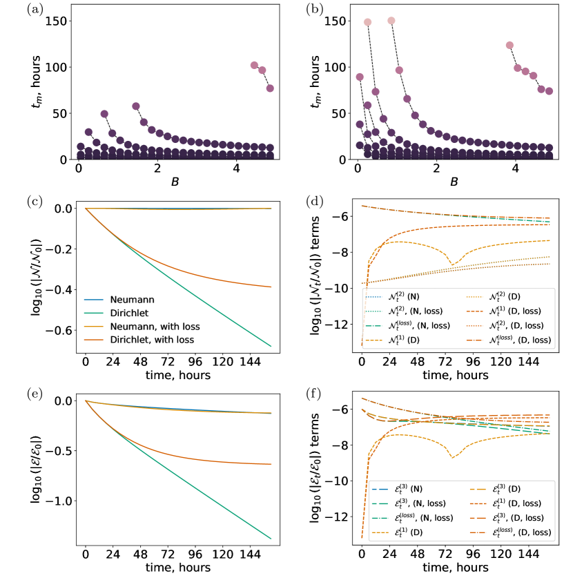
Figure 16: Same as Fig. 6 but compares the higher step size $B=5$ experiments to their equivalents with loss from pitch angle scattering. Note that the outer boundary terms $\mathcal{N}_{t}^{(1)},\mathcal{E}_{t}^{(1)}$ for the loss experiments represent gains as material flows into the domain.

Enhancement location $\mu$: As without loss, a higher $\mu$ means that $t_{m}$ is reached more quickly. Fewer experiments reach monotonicity; those that do reach it more quickly. For the first few hours, the loss experiments actually find that $\mathcal{E}_{t}$ is dominated by reconfiguration - this will be because the enhancement is at higher $L$ so more diffusion is possible. Then loss becomes dominant - for Neumann with loss, the reconfiguration and loss contributions to $\mathcal{E}_{t}$ become comparable after around 70 hours. “Reconfiguration” $\mathcal{E}_{t}^{(3)}$ is not as strong as without loss.

Amplitude $A$: There is no change with amplitude - the same as without loss. We see same overall patterns in $\mathcal{N},\mathcal{E}$ as discussed in previous section.

Enhancement width $\sigma$: Again, a narrower width (i.e. lower $\sigma$) reaches $t_{m}$ quicker, the same as without loss. From $\mathcal{N,E}$ analysis (shown in supplementary materials) we find the same overall results as discussed in Section V.2.1. With loss, the Neumann and Dirichlet runs are more similar to each other than to the runs without loss. With loss, less is lost through the inner boundary.

V.2.4 Outer edge of domain, $L_{outer}$

Without loss, we found that $t_{m}$ varied when we changed the location of a Neumann outer boundary condition, but not a Dirichlet condition. With loss, we find that $t_{m}$ dependence on $L_{outer}$ is very small for both a Neumann boundary (Fig. 17(a)) and a Dirichlet boundary, particularly when the domain boundary and the plasmapause are close (Fig. 17(b))[P1c].

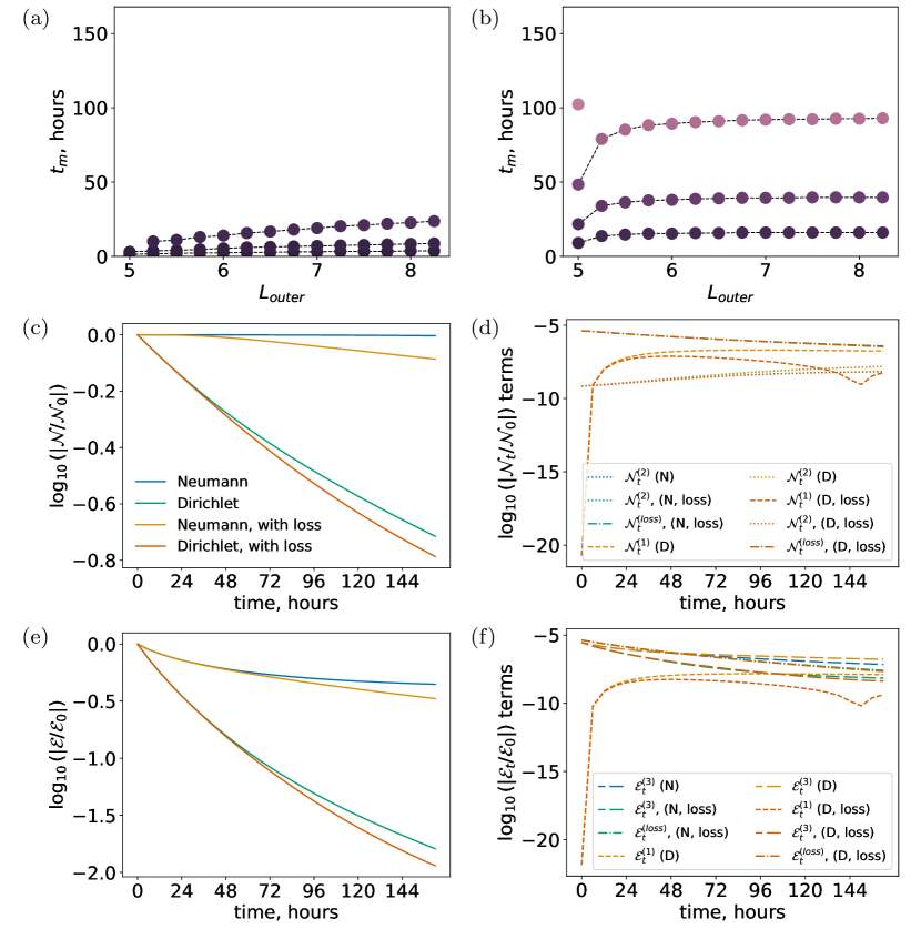
Figure 17: Same as Fig. 16 but investigating the interaction between $L_{outer}$ and loss.

V.2.5 Plasmapause location $L_{p}$

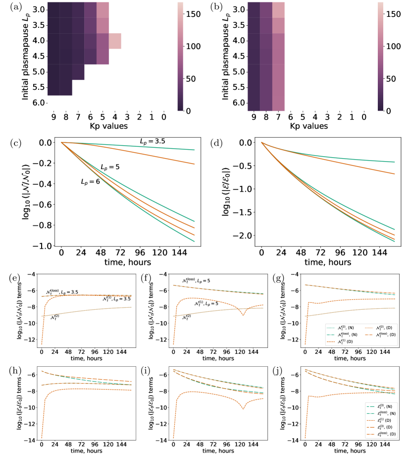
Figure 18: First row: time to monotonicity for Neumann (left) and Dirichlet (right) outer boundary conditions with varying Kp and plasmapause location $L_{p}$. The second row shows the combined $\mathcal{N}$ (c) and $\mathcal{E}$ (d) results for three plasmapause locations, $L_{p}=3.5,5,6$, across a week-long simulation. The third row shows the $\mathcal{N}_{t}$ terms for each of these respectively, and the fourth row shows the $\mathcal{E}_{t}$ terms. Note that outer boundary contributions for $L_{p}=6$ (i.e. $\mathcal{N}^{(1)},\mathcal{E}^{(1)}$) are positive.

When including loss, the extent of the lossy region is a new parameter to consider. The outer limit of this region is the plasmapause, $L_{p}$. Fig. 18(a) and (b) show time to monotonicity across a variety of plasmapause locations. The effect for a Dirichlet outer boundary condition is small, with an effect for the lowest plasmapause values (for which $t_{m}$ is sooner) which quickly drops off to reach a value of $t_{m}$ that no longer changes with $L_{p}$. The effect of plasmaause location with Neumann outer boundary condition is more complex; overall, a plasmapause closer to the Earth reaches monotonicity sooner. However, there is a cut-off in $L$ after which monotonicity is not reached at all.

In Section V.2.2 we noted that $L_{p}>\mu$ could result in the PSD being unable to reach a monotonic state. This relationship is explored by using three plasmapause locations in the $\mathcal{N,E}$ analysis: $L_{p}=3.5,5,6.$ These results are shown in the final three rows of Fig. 18.

As the default enhancement location is $\mu=4$, a plasmapause at $L=3.5$ is at a lower $L$ than the enhancement. Fig. 18(e) indicates that material lost from pitch angle scattering is quickly similar to loss from the outer boundary, and (h) demonstrates that $\mathcal{E}_{t}$ is dominated by the reconfiguration term $\mathcal{E}^{(3)}$ (although this becomes comparable to $\mathcal{E}^{(loss)}$ for the Neumann experiment by the end of the week). With less overall loss, the Neumann and Dirichlet experiments still have distinct values of $\mathcal{N,E}$.

For a plasmapause at $L=5$ or $6$, much more material is lost, as expected since the proportion of particles lost increases with $L$. The norm for $L_{p}=5,6$ is quickly very low (Fig. 18(d)). For $L_{p}=6$, the Neumann experiment reaches a lower energy state, whilst for $L_{p}=5$ the Dirichlet experiment has a lower norm. This is due to more material coming in the outer boundary with a higher $L_{p}$.

For a higher plasmapause location, $\mathcal{E}^{(loss)}$ becomes increasingly larger. When $\mathcal{E}^{(loss)}>\mathcal{E}^{(3)}$, diffusion can not prevent the formation of the extra minimum demonstrated in Section V.2.2. Indeed, this is the relationship observed when plotting several intermediate time instances of the experiments with $L_{p}=3.5,5,6$, shown in Fig. 19. For $L_{p}<\mu$, this minimum does not form (first row of Fig. 19) while the minimum is larger as $L_{p}$ increases (Fig. 19 second and third rows).

Note that since $\mathcal{E}^{(3)_{t}}$ depends on the gradient of the PSD, the growth of this minima (i.e. when $\mathcal{E}^{(loss)}_{t}>\mathcal{E}_{t}^{(3)}$) is dependent on the initial conditions. Loss may or may not dominate the evolution of the system over reconfiguration. Overall, our results emphasise that the plasmapause location relative to the enhancement is important, and that a more distant plasmapause has so much more loss that this can totally change the dynamics [P1b; S1b; S2; S4].

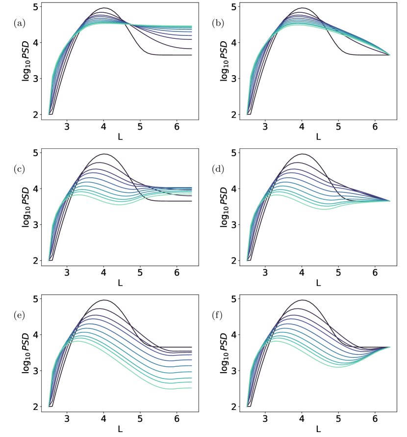
Figure 19: Intermediate phase space density distributions from week long experiments, with a plasmapause $L_{p}$ at $3.5$ (row 1), $L_{p}=5$ (second row) and $L_{p}=6$ (third row). Runs on the left and right have Neumann and Dirichlet outer boundary conditions respectively.

V.3 Summary of Results: The role of the Initial Condition

Monotonicity was easier to obtain when there was already a significant background PSD, corresponding to a large high-$L$ source (i.e. high $B$). Therefore, $t_{m}$ corresponds to the timescale of an enhancement relative to background field. If the enhancement location $\mu$ occurs at high $L$, it doesn’t last as long before the distribution becomes monotonic. Furthermore, a narrower enhancement will be reduced more quickly than a wider one - and using $\mathcal{E}_{t}$, we attributed this to the gradients of the PSD, which will be discussed in Section VI.5. Less intuitively, we found that the time for our enhancement to “fade" into the background varies significantly with the outer boundary location if we used a Neumann boundary. This is a key result, and we explore the consequences of this and future avenues in Section VI.4. Finally, we found that loss from pitch angle scattering has a strong effect on the final shape of the distribution (and therefore the timescale for radial diffusion). Indeed, some numerical experiments never reach monotonicity, casting some questions about future appropriateness of $t_{m}$, which we discuss in Section VI.1 [P1b;S1b;S2;S3a;A2].

Using the evolution of $\mathcal{N}$ we could work out what processes were going on, and from $\mathcal{E}$ we could work out how the system was evolving to reach a maximally-diffused state. We found that although theoretically an experiment with a Neumann OBC can reach a state with a lower $L_{2}$ norm (i.e. zero everywhere), the majority of the time Dirichlet experiments were reaching a state of lower $\mathcal{E}$, because mass could be lost from both boundaries. The Neumann experiments were reaching a state where $\mathcal{E}_{t}\sim 0$; where the dynamics were changing very little once the plateau had risen up, whilst the Dirichlet experiments were still diffusing material from the enhancement by the end of the week [S1b;A1].

Other specific results from the use of $\mathcal{N,E}$ include the importance of gradients in the distribution; using $\mathcal{E}_{t}^{(3)}$ we can estimate the comparative effect of the $L-$dependence of $D_{LL}$ and the gradients in the distributiuon on the evolution of $f$. We found that gradients are more significant, a result worthy of its own discussion section Section VI.5. We can also see in Fig. 12(c) that although using a different domain (i.e. a different $L_{outer}$) does not significantly impact the starting value of $\mathcal{E}$, it does affect the rate at which the system moves towards a steady state (more in Section VI.4, Section VI.2). Finally, we can quantify that loss from pitch-angle scattering has a stronger effect on the evolution of $f$ than radial diffusion does [S4;A2].

VI Discussion: Implications for Future Work

Understanding of the research goals, and the context of our results, has developed throughout the research lifetime of this work. The initial questions shaped the methodology and investigation of the results shaped the narrative of the analysis. Here we put the results into context with existing literature and with future modelling choices. To aid navigation, relevant paragraphs are labelled with our initial research questions in Section III. Each research goal may be addressed in multiple paragraphs.

VI.1 Evaluation of $t_{m}$ and $\mathcal{N,E}$ as analysis tools

Error metrics such as the log-accuracy ratio Morley et al. (2018) are often the first tools considered for comparing distributions; this would be a suitable method to compare the deviation between two distributions, such as between observations and models (although weighting by the Jacobian $1/L^{2}$ may be necessary, as it has been here). When no “truth” is available to compare against, error metrics become an unsuitable tool as it would require a threshold (e.g. when two distributions are “close enough", or when radial diffusion is “done") which would be difficult to motivate objectively. In this section we discuss the performance of tools $t_{m},\mathcal{N,E}$ when comparing distributions and how the distribution morphology became so integral to our analysis.

$t_{m}$ and $\mathcal{N,E}$ are found to be complementary measures of the shape and evolution of the distribution. They are related, as the state of monotonicity and the state of lowest possible $\mathcal{E}$ both have PSDs predominantly weighted towards the outer edge of the domain. $t_{m}$ is a state where the only existing gradients are to the left hand side of the enhancement. Indeed, $\mathcal{E}$ particularly penalises high $f$ at low $L$ (e.g. $f=1$ at at $L=4$ results in a higher $\mathcal{E}$ (1/16) than at $L=5$ (1/25)). (Note, however, that a monotonic distribution can be gaining particles from the outer boundary and therefore in $\mathcal{E}$). Despite the similarity between low-$\mathcal{E}$ and monotonic states, evolution is determined by $\mathcal{E}_{t}$; the steady state reached may not be the lowest $\mathcal{E}$ configuration possible. $\mathcal{E}_{t}$ is in turn usually dominated by reconfiguration term $\mathcal{E}^{(3)}_{t}$, which is an integral across $L$ that is also dependent on $L$. This term tells us that gradients in $f$ (and their location in $L$) are the strongest factors dominating $\mathcal{E}^{(3)}_{t}$. As a result, the distribution will change more rapidly towards the low-$\mathcal{E}$, monotonic-like state when there are steeper gradients, and when those gradients are situated at low $L$.

The dominance of $\mathcal{E}^{(3)}$ consequently suggests that quantities capturing the shape of the distribution and the location of features in it are going to be the most useful tools when analysing the output - as we have found. We conclude that measures using the distribution morphology across the entire domain are necessary to capture the system evolution. Indeed, the outer boundary condition affects the monotonicity of the final state. The shape of the distribution and the ongoing evolution change with the location and condition of the outer boundary. The act of “reducing gradients” means that in general, Neumann experiments reach monotonicity quickly, whilst the steep gradients remaining in the Dirichlet experiments means that they are actually at lower energy states and still changing more rapidly (losing more $L_{2}$ norm and mass) towards a steady state.

We suggest that we finally settled on this pair of tools because they are (a) both domain dependent, and (b) include information about the morphology of the PSD distribution. Both tell us about the entire system, i.e. $\mathcal{E,N}$ tells us about the system across all $L$ at each timestep; $\mathcal{N}_{t},\mathcal{E}_{t}$ inform us about the ongoing evolution of the system at each timestep, and $t_{m}$ is a measure of the long-term evolution. Initially, we searched for domain in-dependent measures; but as the diffusion coefficient $D_{LL}$ is domain dependent, so should be our method of analysis. Both tools relate, predominantly, to gradients. The existence of steep gradients are the largest contributor to a rapidly changing $\mathcal{E}$; a distribution rapidly heading towards a steady state. A moderate limitation of $\mathcal{N,E}$ is that one can only use idealised diffusion coefficients rather than the empirical ones from Ozeke et al. (2014) used in calculating $t_{m}$. Unfortunately, a limitation of $t_{m}$ is that some parameter combinations never reach a monotonic state, i.e. once loss is included at higher $L$ values (see Section V.2.2 and Fig. 19). The extra minimum in these cases suggest that we may need to characterise by convexity (i.e. number and location of extrema) rather than simply monotonicity and $t_{m}$. Nevertheless, we found $t_{m}$ to be an extremely useful measure to compare the different experiments, which could be related back to radiation belt processes, to a “quiet” state and to quantifiable properties of the PSD $f$. Using both $t_{m}$ and $\mathcal{N,E}$ together gives us a nuanced description of timescale (Section VI.2). These quantities allowed us a clear and efficient means of comparing experiments and understanding the processes behind the evolution of each [S3a;S3b]

VI.2 Timescale for radial diffusion

A radial diffusion “timescale" is poorly defined when $D_{LL}$ depends on $L$; one cannot simply take $\frac{1}{D_{LL}}$ as the characteristic timescale. This is an open question both for idealised models and the real radiation belts, because of the number of underlying approximations. Potential measures of timescale include the autocorrelation, or dimensional analysis of self similar solutions (e.g. Osmane and Lejosne (2021)). Unfortunately, self similar timescales are difficult to find for the 1D radial diffusion equation Eq. 1 with diffusion coefficients Eq. 2 or Eq. 5 because of the high order of $L$. Typically, one makes “by eye" judgments of storm time radiation belt simulations. One could numerically solve for the equilibrium solution and then find the time taken to reach this (e.g. Ripoll et al. (2016)) but this will also depend on the metric or threshold one chooses to define as close enough to this equilibrium solution. Alternatively, suggestions were to take either the minimum or maximum $1/D_{LL}$ in the system, as this would at least give you a “fastest possible” timescale (various personal communications). We have explored methods of quantifying timescale using our tools.

Using $t_{m}$, the concept of timescale reduces to “how long until an enhancement is diffused away". The results in Section V.1 thereby include how the initial condition (e.g. size and location of enhancement) relate to timescale without loss. There is a large variability with Kp$,B,\mu$ etc. From $t_{m}$ at a Kp of 4-5 we conclude that the timescale is on the order of days, or tens of hours (for all the $t_{m}$ plots together, see Figure S1). Some combinations of initial conditions will keep this close to one day, others closer to a week. This definition is not particularly suited once one considers loss from pitch angle scattering; although the timescale drops to hours or days, since monotonicity is no longer guaranteed it is a poor indicator of timescale [P2a,b,c].

$\mathcal{E}$ is even less suited to extracting a timescale as one would need to set a threshold. Nevertheless, we can draw some qualitative conclusions. Without loss, within a few days we see that the Neumann ensembles for all initial conditions have a relatively flat $\mathcal{E}$ - the dynamics are not changing. On the other hand, most Dirichlet experiments are still reducing in $\mathcal{E}$ at this point. Obviously this timescale is difficult to use as it has such a strong dependence on the outer boundary condition - which reflects the importance of the outer boundary condition. With loss, we see that initial conditions matter far less; with 72 hours most ensemble members have reached a very low energy, even though they are still losing mass; the timescale of the dynamic processes is only a few days before becoming “quiet" [P2a].

Our measures of timescales tell us (a) when the enhancement is diffused to the background via $t_{m}$ (although needs adapting for the case with loss) and (b) whether the dynamics are still changing (i.e. whether there are rapidly changing gradients being diffused away) via $\mathcal{E,E}_{t}$. We find that pitch angle loss generally dominates over the radial diffusion timescale (and note that in practice, pitch angle scattering timescales also vary with $L$ and energy, Ripoll et al. (2016)).

As a result, from our work we can suggest only that the radial diffusion timescale is on a scale of hours to days, depending on the parameters one uses (e.g. Kp, $\mu$ etc). We note that using either the minimum or maximum value of $\frac{1}{D_{LL}}$ is not a good indicator of timescale, for two reasons: (a) our conclusion that one should consider the entire domain, and (b) our result that gradients in the PSD affect the evolution of the system more than the value of $D_{LL}$, at least for a reasonable activity magnetosphere ($Kp=4$) and up to $L=6.5$. The definition of timescale is also still poorly defined and should be specified for a given purpose in order for any quantitative conclusions to be reached, e.g. time for an enhancement to be diffused away, for the radiation belts to drop below a certain energy, or return to a specific state. One interesting potential timescale would be the time taken for loss or reconfiguration terms ($\mathcal{E}^{(loss)}$, $\mathcal{E}^{(3)}$) to dominate evolution (i.e. to be the dominant term of $\mathcal{E}_{t}$) [P2a;P2b;A3].

VI.3 Ensembles for radiation belt modelling

The goal of ensemble modelling needs to be more carefully specified, before a method of comparing ensemble members can be analysed. For example, an error metric would work to compare variation from a “truth" (e.g. observation) or from a baseline forecast (i.e. before one creates ensemble members by varying parameterisations). We make several observations on ensemble modelling for future use.

A simple use of ensemble modelling would be to sample unknown quantities. Our results suggest that this would need to be done carefully to avoid bias; for example, sampling a range of $\mu$ values would err on the of faster diffusion and earlier monotonicity, because $t_{m}$ does not change linearly with $\mu$. Furthermore, one should be wary of determining an “average" from an ensemble; simply averaging PSD values at each $L$ across many ensemble members would not be meaningful when one needs to consider the whole domain first. This domain dependence raises a further problem; given an $L$-dependent $D_{LL}$, there is no clear way to compare simulations with a different outer boundary location or condition.

Finally, we note that one possible goal for ensemble modelling could be to characterise the influence of chaotic or stochastic processes. This would need to be carefully thought through, using the inherent properties of such a complex system; simply sampling from the initial conditions above (or from similar values of $D_{LL}$, Thompson et al. (2020)) is not likely to represent either a chaotic or stochastic underlying nature, but only to reinforce any bias towards higher amounts of diffusion. Poorly defined averaging of underlying properties may be why existing diffusion coefficients vary drastically Murphy et al. (2023).

In Section IV.2 we motivated $t_{m}$ by considering the properties required of a metric to analyse our ensemble. We note that our additional, analytic tools $\mathcal{E,N}$ meet the proposed initial requirements (i.e. excluding the requirement for insensitivity to the total particle population) and suggest that these requirements may be useful in finding other qualitative tools for analysing ensembles [A1].

We conclude that $t_{m}$ and $\mathcal{N,E}$ are good tools for qualitatively understanding what an ensemble is doing, but not necessarily a good tool for comparing ensemble members for modelling or forecasting purposes [P1a;S3b].

VI.4 The Simulation Outer Boundary

We used both Neumann and Dirichlet outer boundary conditions as both have physical motivations. We tested multiple $L_{outer}$ options as the true radiation belt outer boundary is both poorly defined, since particles don’t stop existing beyond the last closed drift shell and poorly represented in current models, which often place the outer boundary where observations exist - far short of the true outer boundary. We have found that both the outer boundary location and condition affects the evolution of the system and the final PSD distribution after a week. The outer boundary condition used in our experiments to identify this effect is very idealised; here we discuss what impacts this may have on outer boundaries used in practice.

$t_{m}$ showed a clear difference between Neumann and Dirichlet conditions; Neumann conditions reached monotonicity first. $t_{m}$ also varied with the choice of $L_{outer}$, especially for a Neumann boundary without loss from pitch angle scattering but also for a Dirichlet condition with loss, when the plasmapause is nearby. Using $\mathcal{N,E}$ we also found differences with both outer boundary location and condition. We expected a different long term solution for Neumann and Dirichlet conditions, and found that evolution towards these steady states was very different (i.e. Neumann could reach a lower-$\mathcal{E}$ state, but Dirichlet lost $\mathcal{E}$ more quickly, heading towards their steady state more rapidly). While the initial $\mathcal{E}$ did not change significantly with $L_{outer}$, the evolution of $\mathcal{E}$ did vary; a smaller $L_{outer}$ (and hence a shorter domain) had $\mathcal{E}$ that diverged more with time between Neumann and Dirichlet outer boundary conditions. Loss mitigated, but did not remove, the differences between simulations with outer boundary location and condition. We conclude that if these options give different dynamics and different PSD distributions over the week, then we need to find the correct boundary conditions. [P1c,S1a,S1b]

Typically, models of the outer radiation belt use a Dirichlet outer boundary to make use of spacecraft observations. These are at positions well short of the true outer edge of the radiation belt, for example they may be curtailed to $L_{outer}=5.5$ Glauert et al. (2014) or extrapolated to higher $L$ values Subbotin and Shprits (2009); Shprits et al. (2006).Footnote: This is also close to the typical plasmapause location, which interacts with OB location and condition. Unfortunately, most missions are limited to a few years; for a consistent set of flux observations, one must use geostationary data, for example GOES, observed daily between $L=5.9$ and $6.4$ but mapped to a constant $L$ to enable modelling Glauert et al. (2018). Whilst at first this appears to be more physical than the idealised boundary conditions tested in this work, we have identified that just the inclusion of observations does not remove all the problems associated with the outer boundary [S1d].

Either outer boundary condition, imposed incorrectly, can correspond to erroneous sinks or sources. For example, in our experiments, a Dirichlet condition where the outer boundary value is higher than in the bulk of the simulation domain represents an infinite source of material. Since our Neumann boundary experiments have a plateau that can freely rise, this actually represents an increased source at the outer boundary - which is also not physical. Using a data-driven outer boundary (such as used in most real-life models) would reduce the imposition of unphysical sinks and sources, but we have shown that it does not resolve the problem as these boundaries are placed at a low $L_{outer}$ that curtails the domain, resulting in different evolution (as we are removing the stronger high-$L$ diffusion). The effect of this curtailment changes with outer boundary condition (see e.g. the diverging $\mathcal{E}_{t}$ in Fig. 12(c,e)). From Fig. 17 it’s clear that once one includes loss from pitch angle scattering, the evolution differences between outer boundary conditions is reduced, but the shape of the distribution still changes with $L_{outer}$, as $t_{m}$ is not independent of $L_{outer}$. Using an outer boundary location determined by the different trajectories of different spacecraft is not ideal - the model corresponding to each spacecraft would then have a different $L_{outer}$, and each of these models would respond differently, reaching monotonicity at different times, because outward radial diffusion is not being properly captured.[P1c,S1b]

Would using observations at every timestep sufficiently constrain the simulation so as to remove the variability we see when changing $L_{outer}$ and the outer boundary condition? This is not clear. It may be that using observations approximates the missing outer boundary processes well enough. However, whilst relying on observations to correct improper boundary conditions may perform well for event reproduction (i.e. hindcasting), observations are naturally not available for the future. This may limit how far in advance we can model radiation belt behaviour. Neither Neumann nor Dirichlet boundary conditions are suitable for predictive purposes. Ideally we would not have to pick between these when we do not have clear values with which to constrain this outer boundary (as is the case here). Currently, we are reduced to comparing empirically which simulation settings account for variation across more orders of magnitude, rather than solely using physical motivations [S1d].

Options would therefore be to used mixed (Robin) boundaries that relate the flux from the domain to the outer boundary values, and/or some way to include the observations in the middle of the domain such as data assimilation or source terms. Methods such as these are already under investigation to resolve the fact that current modelling misses processes such as dropouts Cervantes et al. (2020) [S1a,S1c].

However, even a Robin boundary condition would not fix the fact that a true outer boundary location is both difficult to define and difficult to find. One could find the empirical extent of the highly-charged particles. However, this is not the same as the last closed drift shell (LCDS), which is the outer limit of adiabatically trapped particles. Particles within a closed drift shell will continue to drift on their path (of constant magnetic field) around the Earth. However, if a drift shell is open then sections of the drift path lie on open field lines outside the magnetosphere. Here, particles can be lost to the solar wind. The last closed drift shell is the last point in which particles are trapped rather than being lost to the solar wind. Therefore the LCDS could be considered the “true" edge of the diffusion domain (but not the edge of the particle population) [S1a].

There is significant uncertainty in the location of the LCDS as modelled using state-of-the-art global magnetosphere models (e.g. Albert et al. (2018)) and there is significant variability in the location of the LCDS (e.g. Bloch et al. (2021)) due to motion of the magnetopause and spatiotemporal variability of the magnetic field in Earth’s outer magnetosphere. Bloch et al. (2021) estimated the typical outer boundary to be at $L^{*}\sim 8R_{E}$ - significantly more distant than models used in practice [S1d].

In this work we have shown that in simulations, both the outer boundary condition and location change the rate of evolution and the shape of the phase space density distribution. We have argued that using a curtailed domain to set a Dirichlet outer boundary may remove these problems for historical event studies, but are not suitable for predictive purposes. Finally, as radial diffusion is about the diffusion of particles across different drift paths, radial diffusion is not well defined when drift paths are open. Therefore a theoretical limit to the radiation belts is the last closed drift shell (LCDS). However, this is (a) a dynamic boundary, (b) difficult to identify in practice, (c) not a closed outer boundary (i.e. particles can be lost to or gained through it) and (d) still an approximation, as in reality the last closed drift orbits are not uniquely defined. It may be impossible to set a “true” outer boundary; in the meantime we do not know what level of accuracy is needed in the outer boundary location and conditions to adequately reflect the radiation belts. We conclude that significant work is required to identify reasonable outer boundary conditions and location for modelling; the outer boundary in real life is very variable, and we have shown that simulations are sensitive to several outer boundary choices [S1a,c,d].

VI.5 Improving $D_{LL}$ vs improving PSD distribution

The overwhelming recent focus to improve radial diffusion is through the diffusion coefficient $D_{LL}$, for example the theory behind $D_{LL}$ Lejosne and Albert (2023), the strength of the electromagnetic perturbations driving $D_{LL}$ (both generally, Bentley et al. (2020) , or for event specific diffusion coefficients Silva et al. (2022); Li et al. (2020) ), parameterisations of $D_{LL}$ for use operationally Murphy et al. (2023), the effect of plumes on diffusion coefficients Sandhu et al. (2023), or even radial diffusion vs radial transport Osmane et al. (2023). However, our results suggest that the gradients of the underlying phase space density distribution may have more effect on the radial diffusion [A2].

Comparatively less effort has gone into finding the underlying PSD distribution. Typically, this is built up on a case-by-case basis for event studies, or to specifically understand the mechanism behind enhancements, rather than as a foundation for radiation belt modelling. There are many difficulties with the construction of radial PSD profiles, particularly as these are made from observations which are sparse in time and space, often on scales much slower than enhancements Kim et al. (2023a). Turner et al. (2012) includes a statistical study and emphasises the need to include error and uncertainty. Our results above (Section V.1.4) indicate that it is the gradients in the radial profile, rather than the exact $D_{LL}$, that determines radial diffusion, to several orders of magnitude. We have not explored the extent of this result: if there is a limit to this with a stronger L dependence, a longer domain or the choice of boundary condition. Nevertheless, as radial diffusion is the large scale, bulk mechanism behind radiation belt evolution, and recent PSD profiles are shown to regularly contain gradients from enhancements Chen et al. (2020); Kim et al. (2023b, a), finding the radial PSD profiles may be a more valuable future route of study; the form of $D_{LL}$ may be less important than getting the gradients of local enhancements right. However, given that the uncertainty in $D_{LL}$ is also of orders of magnitude, improved $D_{LL}$s are still likely to result in improved radiation belt modelling.

VI.6 Limitations of our numerical experiments

The strengths and weaknesses of our study arise from the same principle: idealised experiments. By examining the fundamentals of radial diffusion modelling we aimed to understand the results of ensembles. To do so, we made many simplifications, which we shall review.

Our experiments showed that the “background” initial condition used above should be skewed further to lower $L$, for example the final monotonic distributions shown in Fig. 4, rather than the step-and-bump of our initial conditions. The “background” higher PSD at the outer boundary is assumed to be from substorms. Given that the inter-substorm time is relatively fast, with a mode of 3 hours (Freeman and Morley (2004); Keiling et al. (2022)), this “background” level is a reasonable initial condition. We also used a Gaussian to represent an enhancement. However, if the enhancements occur on the order of days, single events (and therefore “time for an enhancement to diffuse away”) should be replaced by compounded events Kim et al. (2023b).

We did not explore the result of variance of the inner boundary. While the outer boundary condition and location have been thoroughly explored, they are unrealistic. They do not include observations as per most operational models and despite being able to physically motivate these settings initially, they essentially relate to an unphysical source or sink at the boundary. This poses several questions about how radiation belt modelling should be attempted in future, which are covered in Section VI.4; a different methodology than ours would be needed to investigate these questions, and to examine the relative effect of different driving conditions at the outer boundary, which was out of the scope of this investigation.

The radial diffusion equation Eq. 7 is well-known and widely used. Our results confirm that it may not be meaningful to consider radial diffusion without loss from pitch angle scattering. Our equation for loss is very simple, in order to match the number of parameters used in our experiments; more sophisticated parameterisations exist (e.g. Orlova et al. (2016)). To keep our problem tractable, we also only considered a single value for the first and second adiabatic invariants. A downside of our simple loss equation is the lack of time dependence; unlike real life, the amount of particles lost does not vary, except when we set a different plasmapause location. Of course, exploring all these options is a difficult problem; in order for the problem to remain tractable, we chose not to vary these.

A major choice in this investigation was the Ozeke and idealised versions of $D_{LL}$, Eq. 2 and Eq. 5. Unfortunately we could not use a single $D_{LL}$ throughout the investigation; whilst the Ozeke model is a simple parameterisation that is widely used operationally, it does not admit easy solutions for $\mathcal{N}_{t}$ and $\mathcal{E}_{t}$. The parameterisation of Kp is very rough and is a coarse average over many different processes that all affect radial diffusion (e.g. ULF waves, compressions, plumes). Nevertheless, both models are comparable to diffusion coefficients used elsewhere. The assumption that some form of radial diffusion is always ongoing is a reasonable one as there is always some level of ULF waves; other limitations of radial diffusion modelling can be found in Bentley et al. (2019).

Despite the large number of idealisations required for this work, we nevertheless reached some general and significant conclusions that will inform future ensemble modelling and suggest that new directions are needed for radiation belt modelling. These are summarised below.

VII Conclusion

We used numerical experiments to investigate how initial conditions and basic radial diffusion modelling techniques affect the final phase space density of radiation belt ensembles. As yet, there are few standard methods of analysing ensembles, hence we explore some in this work. Despite the radial diffusion equation arising from the simple heat equation, the space and time dependence of the diffusion coefficient $D_{LL}$ make analysis of this system rather complicated, even while space weather modelling demands are increasing. Our initial goals included defining a radial diffusion timescale and the effect of model settings across ensemble members, yet as part of this work we have identified significant questions in current practice for radiation belt modelling. To aid navigation of this paper, each goal has been explicitly stated in Section III and tagged throughout.

The key findings are summarised here and briefly expanded below:

1. Evolution of the system depended on the outer boundary condition and location. A shorter domain evolved at a different rate than a longer one; this will be due to the $L$ dependence of $D_{LL}$. It is not clear what outer boundaries should be used and this may have consequences for modelling the radiation belts [P1c;S1].

2. Using an analytical quantity (the energy moment, or norm $\mathcal{E}$) we found that the gradient of the phase space density distribution contributed more to the evolution of the system than the diffusion coefficient $D_{LL}$ [A2].

3. Flaws in typical metrics included (a) threshold-based metrics which gave results highly threshold-dependent, and (b) the requirement of a $\frac{1}{L^{2}}$ Jacobian factor due to the co-ordinate system [P1a].

4. Time to monotonicity $t_{m}$ and mass / energy moments $\mathcal{N},\mathcal{E}$ were developed to analyse radial diffusion models [P1a].

   • These metrics were appropriate because they consider the whole domain and are $L$ dependent,

   • $t_{m}$ is intuitively interpretable as time for an enhancement to diffuse away [S2],

   • the system can be considered as continually moving to a low energy moment (or $L_{2}$ norm) $\mathcal{E}$ state [A1],

   • $\mathcal{N},\mathcal{E}$ could be easily adapted to other radiation belt models [S1].

5. Loss from pitch angle scattering generally dominated over radial diffusion [S4].

6. Ensembles varying the enhancement location would be biased towards additional radial diffusion [P1b,S3].

The methodology of this study was to perturb simulations, selecting ensemble members based on sampling idealised conditions from Earth’s radiation belts. Initial conditions were a “background” phase space density (PSD) distribution, plus a localised enhancement. These properties were varied and their impact on the evolving PSD distribution assessed using time to monotonicity $t_{m}$ and two analytic mass- and energy-like quantities $\mathcal{N,E}$. Multiple physical outer boundary conditions and locations were tested, using both empirically fitted and idealised radial diffusion coefficients. Finally, loss from pitch angle scattering was included. Throughout this paper, the impact of all these factors on the PSD have been extracted. Here we summarise significant findings and important discussions.

The final PSD, and evolution towards that state, varied with both the outer boundary condition and location. Both constant flux (Neumann) and fixed value (Dirichlet) outer boundaries can be physically motivated, although neither can be easily implemented to reflect real-life conditions. Current operational methods generally involve either a diffusion domain shortened to where observations are available, or extrapolations from this point to a distant outer boundary. We have shown that while observations could constrain simulation errors from a curtailed boundary for historical events, this is far from assured when modelling future behaviour. The interplay of domain-dependent $D_{LL}$ and outer boundary condition and location as an additional source of error has not been heretofore considered. We suggest several ways forward, including mixed boundaries and data assimilation. Our work also suggests that identifying an outer edge to the real radiation belts - currently poorly defined and difficult to identify from observations - will have significant implications for modelling. In particular, as modelling of the radiation belts becomes more realistic, the outer boundary location (and therefore the size of the domain) will vary more in time in our model [P1c;S1a;S1b;S1c;S1d;S2e].

The bulk of previous work on improving radial diffusion estimates has focused on finding and characterising $D_{LL}$. By comparing the components of $\mathcal{E}_{t}$, which determines the ongoing evolution of the system, we find that it is instead the gradients of the PSD distribution that determine the ongoing amount of diffusion. This result also emphasises the need to integrate any comparative measures across the entire domain to capture the full impact of the $L$ dependence of radial diffusion. Diffusion is not well characterised by either the largest or smallest $D_{LL}$ in the domain [A2;A3].

Upon analysis of our measures $t_{m}$ and $\mathcal{N,E}$, we find that their effectiveness is partly due to their relationship to gradients and hence the morphology of the PSD distribution. Our two measures are related, yet complementary. Together they include information on both the system state and the ongoing diffusion. They are both interpretable; $t_{m}$ has a clear physical interpretation (how long until an enhancement has been completely diffused away) while the components of $\mathcal{N}$ and $\mathcal{E}$ describes the mass in the simulation and the ongoing evolution to a steady state respectively. Using an idealised diffusion coefficient in $\mathcal{N,E}$ enables an explicit comparison of the inner boundary, outer boundary and loss terms on the system. A limitation of $\mathcal{N,E}$ is the requirement of an idealised $D_{LL}$, whilst ideally $t_{m}$ should be adapted to enable better application for loss from pitch angle scattering. These are excellent tools for qualitatively understanding what an ensemble is doing, but they are not error metrics. For error metrics it is likely that $L$ will need to be accounted for, e.g. with the Jacobian $1/L^{2}$. Both measures are domain- and boundary type-dependent; this is a desirable property as it highlights the fact that for radial diffusion, different domain sizes and boundary types are effectively modelling different physical systems [P1a;P1b;P2a;S2;S3;A1].

Using $t_{m}$ and $\mathcal{N,E}$ all the components of a typical radial diffusion model were compared. Loss from pitch-angle scattering (using an extremely simple loss model) generally had more effect on the PSD distribution than diffusion, although this was highly dependent on the location of the plasmapause. A more distant plasmapause results in so much more loss that the dynamics could change totally, and the system never be able to reach a monotonic state. Of the initial condition, step size parameterised by $B$ (corresponding to the quiet background PSD distribution) and enhancement location $\mu$ had the greatest effect on the timescale of diffusion and the state of the system; these results agree with our findings that gradients control the diffusion. Roughly, we found that $\text{loss}>\text{outer boundary}>\text{initial condition}>\text{inner boundary}$ for the impact on evolution, by order of magnitude; extreme values change this ordering. The initial condition controlled loss at the inner boundary [P2c;S3;S4;A1].

To summarise, in this paper we have presented a methodology to analyse the components of a numerical model of radial diffusion in Earth’s radiation belt and compare the impact of those components on the shape and evolution of the particle phase space density distribution. Our work emphasises the need to consider the entire modelling domain when comparing or analysing radial diffusion simulations. Furthermore, we find that the $L$-dependence of the diffusion coefficient results in a model that is domain dependent; curtailing the outer boundary or using inappropriate boundary conditions effectively models very different systems. We make several suggestions for the outer boundary in future models. We find that it is the gradients of the phase space density that mainly control diffusion, contrary to the focus of most radial diffusion studies on $D_{LL}$.

Data Availability Statement

Data generated in support of this paper will be uploaded to an online repository with a DOI after first review.

References

- Tu et al. (2014) W. Tu, G. S. Cunningham, Y. Chen, S. K. Morley, G. D. Reeves, J. B. Blake, D. N. Baker, and H. Spence, Geophysical Research Letters 41 (2014), 10.1002/2013GL058819.
- Ozeke et al. (2017) L. G. Ozeke, I. R. Mann, K. R. Murphy, D. G. Sibeck, and D. N. Baker, Geophysical Research Letters 44 (2017), 10.1002/2017GL072811.
- Huang et al. (2010) C.-L. Huang, H. E. Spence, M. K. Hudson, and S. R. Elkington, Journal of Geophysical Research: Space Physics 115, n/a (2010).
- Liu et al. (2016) W. Liu, W. Tu, X. Li, T. Sarris, Y. Khotyaintsev, H. Fu, H. Zhang, and Q. Shi, Geophysical Research Letters 43, 1023 (2016).
- Thompson et al. (2020) R. L. Thompson, C. E. J. Watt, and P. D. Williams, Journal of Geophysical Research: Space Physics 125 (2020), 10.1029/2019JA027254.
- Sarma et al. (2020) R. Sarma, M. Chandorkar, I. Zhelavskaya, Y. Shprits, A. Drozdov, and E. Camporeale, Journal of Geophysical Research: Space Physics 125 (2020), 10.1029/2019JA027618.
- Balasis et al. (2023) G. Balasis, M. A. Balikhin, S. C. Chapman, G. Consolini, I. A. Daglis, R. V. Donner, J. Kurths, M. Paluš, J. Runge, B. T. Tsurutani, D. Vassiliadis, S. Wing, J. W. Gjerloev, J. Johnson, M. Materassi, T. Alberti, C. Papadimitriou, P. Manshour, A. Z. Boutsi, and M. Stumpo, “Complex systems methods characterizing nonlinear processes in the near-earth electromagnetic environment: Recent advances and open challenges,” (2023).
- Morley (2020) S. K. Morley, Space Weather 18 (2020), 10.1029/2018SW002108.
- Hua et al. (2023) M. Hua, J. Bortnik, A. C. Kellerman, E. Camporeale, and Q. Ma, Space Weather 21 (2023), 10.1029/2022SW003234.
- Watt et al. (2022) C. E. Watt, H. J. Allison, S. N. Bentley, R. L. Thompson, I. J. Rae, O. Allanson, N. P. Meredith, J. P. Ross, S. A. Glauert, R. B. Horne, S. Zhang, K. R. Murphy, D. Rasinskaitė, and S. Killey, Frontiers in Astronomy and Space Sciences 9 (2022), 10.3389/fspas.2022.1004634.
- Shprits et al. (2013) Y. Shprits, A. Kellerman, D. Kondrashov, and D. Subbotin, Geophysical Research Letters 40 (2013), 10.1002/grl.50969.
- Hands et al. (2018) A. D. Hands, K. A. Ryden, N. P. Meredith, S. A. Glauert, and R. B. Horne, Space Weather 16 (2018), 10.1029/2018SW001913.
- Matéo-Vélez et al. (2018) J. C. Matéo-Vélez, A. Sicard, D. Payan, N. Ganushkina, N. P. Meredith, and I. Sillanpäa, Space Weather 16 (2018), 10.1002/2017SW001689.
- Roederer and Zhang (2014) J. G. Roederer and H. Zhang, Dynamics of Magnetically Trapped Particles, Vol. 403 (2014).
- Walt (2005) M. Walt, Introduction to geomagnetically trapped radiation (Cambridge University Press, 2005).
- Reeves et al. (2012) G. D. Reeves, Y. Chen, G. S. Cunningham, R. W. H. Friedel, M. G. Henderson, V. K. Jordanova, J. Koller, S. K. Morley, M. F. Thomsen, and S. Zaharia, Space Weather 10, n/a (2012).
- Beutier and Boscher (1995) T. Beutier and D. Boscher, Journal of Geophysical Research: Space Physics 100 (1995), 10.1029/94ja03066.
- Glauert et al. (2014) S. A. Glauert, R. B. Horne, and N. P. Meredith, Journal of Geophysical Research: Space Physics 119, 268 (2014).
- Subbotin and Shprits (2009) D. A. Subbotin and Y. Y. Shprits, Space Weather 7, 1 (2009).
- Thompson et al. (2021) R. L. Thompson, S. K. Morley, C. E. Watt, S. N. Bentley, and P. D. Williams, Space Weather 19 (2021), 10.1029/2020SW002602.
- Lejosne and Albert (2023) S. Lejosne and J. M. Albert, Frontiers in Astronomy and Space Sciences 10 (2023), 10.3389/fspas.2023.1200485.
- Green and Kivelson (2004) J. C. Green and M. G. Kivelson, Journal of Geophysical Research: Space Physics 109 (2004), 10.1029/2003JA010153.
- Reeves et al. (2013) G. D. Reeves, H. E. Spence, M. G. Henderson, S. K. Morley, R. H. W. Friedel, H. O. Funsten, D. N. Baker, S. G. Kanekal, J. B. Blake, J. F. Fennell, S. G. Claudepierre, R. M. Thorne, D. L. Turner, C. A. Kletzing, W. S. Kurth, B. A. Larsen, and J. T. Niehof, Science 341, 991 (2013).
- Lejosne and Kollmann (2020) S. Lejosne and P. Kollmann, Space Science Reviews 216, 19 (2020).
- Falthammar (1968) C.-G. Falthammar (Reinhold Book Corporation, 1968) pp. 157–169.
- Lejosne (2019) S. Lejosne, Journal of Geophysical Research: Space Physics 124, 4278 (2019).
- Osmane and Lejosne (2021) A. Osmane and S. Lejosne, The Astrophysical Journal 912 (2021), 10.3847/1538-4357/abf04b.
- Brautigam et al. (2005) D. H. Brautigam, G. P. Ginet, J. M. Albert, J. R. Wygant, D. E. Rowland, A. Ling, and J. Bass, Journal of Geophysical Research: Space Physics 110, 1 (2005).
- Fei et al. (2006) Y. Fei, A. A. Chan, S. R. Elkington, and M. J. Wiltberger, Journal of Geophysical Research 111, A12209 (2006).
- Olifer et al. (2019) L. Olifer, I. R. Mann, L. G. Ozeke, I. J. Rae, and S. K. Morley, Journal of Geophysical Research: Space Physics , 2018JA026348 (2019).
- Sandhu et al. (2021) J. K. Sandhu, I. J. Rae, J. R. Wygant, A. W. Breneman, S. Tian, C. E. Watt, R. B. Horne, L. G. Ozeke, M. Georgiou, and M. T. Walach, Journal of Geophysical Research: Space Physics 126 (2021), 10.1029/2020JA029024.
- Bentley et al. (2019) S. N. Bentley, C. E. Watt, I. J. Rae, M. J. Owens, K. Murphy, M. Lockwood, and J. K. Sandhu, Space Weather 17, 599 (2019).
- Ozeke et al. (2012) L. G. Ozeke, I. R. Mann, K. R. Murphy, I. J. Rae, D. K. Milling, S. R. Elkington, A. A. Chan, and H. J. Singer, Journal of Geophysical Research: Space Physics 117, 1 (2012).
- Ozeke et al. (2014) L. G. Ozeke, I. R. Mann, K. R. Murphy, I. J. Rae, and D. K. Milling, Journal of Geophysical Research: Space Physics 119, 1587 (2014).
- Matzka et al. (2021) J. Matzka, C. Stolle, Y. Yamazaki, O. Bronkalla, and A. Morschhauser, Space Weather 19 (2021), 10.1029/2020SW002641.
- Drozdov et al. (2021) A. Y. Drozdov, H. J. Allison, Y. Y. Shprits, S. R. Elkington, and N. A. Aseev, Journal of Geophysical Research: Space Physics 126 (2021), 10.1029/2020JA028707.
- Murphy et al. (2023) K. R. Murphy, J. Sandhu, I. J. Rae, T. Daggitt, S. Glauert, R. B. Horne, C. E. Watt, S. Bentley, A. Kellerman, L. Ozeke, A. J. Halford, S. Tian, A. Breneman, L. Olifer, I. R. Mann, V. Angelopoulos, and J. Wygant, Space Weather 21 (2023), 10.1029/2023SW003440.
- Silva et al. (2022) G. B. Silva, L. R. Alves, W. Tu, A. L. Padilha, V. M. Souza, L. F. Li, X. Lyu, and M. B. Pádua, Journal of Geophysical Research: Space Physics 127 (2022), 10.1029/2022JA030602.
- Lyons et al. (1972) L. R. Lyons, R. M. Thorne, and C. F. Kennel, Journal of Geophysical Research 77 (1972), 10.1029/ja077i019p03455.
- Li et al. (2022) L. Y. Li, J. Yu, J. B. Cao, L. J. Chen, G. D. Reeves, and J. B. Blake, “Competitive influences of different plasma waves on the pitch angle distribution of energetic electrons inside and outside plasmasphere,” (2022).
- Orlova et al. (2016) K. Orlova, Y. Shprits, and M. Spasojevic, Journal of Geophysical Research: Space Physics 121 (2016), 10.1002/2015JA021878.
- Shprits et al. (2007) Y. Y. Shprits, N. P. Meredith, and R. M. Thorne, Geophysical Research Letters 34 (2007), 10.1029/2006GL029050.
- Welling et al. (2012) D. T. Welling, J. Koller, and E. Camporeale, Geoscientific Model Development 5 (2012), 10.5194/gmd-5-277-2012.
- Tadjeran (2007) C. Tadjeran, Communications in Numerical Methods in Engineering 23 (2007), 10.1002/cnm.879.
- Bloch et al. (2021) T. Bloch, C. E. Watt, M. J. Owens, R. L. Thompson, and O. Agiwal, Earth and Space Science 8 (2021), 10.1029/2020EA001610.
- Strauss (2007) W. Strauss, “Partial differential equations: An introduction, 2nd edition,” (2007).
- Kendon et al. (2001) V. M. Kendon, M. E. Cates, I. Pagonabarraga, J. C. Desplat, and P. Bladon, Journal of Fluid Mechanics 440 (2001), 10.1017/S0022112001004682.
- Stratford et al. (2005) K. Stratford, R. Adhikari, I. Pagonabarraga, and J. C. Desplat (2005).
- Morley et al. (2018) S. K. Morley, T. V. Brito, and D. T. Welling, Space Weather 16 (2018), 10.1002/2017SW001669.
- Ripoll et al. (2016) J. F. Ripoll, V. Loridan, G. S. Cunningham, G. D. Reeves, and Y. Y. Shprits, Journal of Geophysical Research: Space Physics 121 (2016), 10.1002/2015JA022207.
- Shprits et al. (2006) Y. Y. Shprits, R. M. Thorne, R. Friedel, G. D. Reeves, J. Fennell, D. N. Baker, and S. G. Kanekal, Journal of Geophysical Research: Space Physics 111 (2006), 10.1029/2006JA011657.
- Glauert et al. (2018) S. A. Glauert, R. B. Horne, and N. P. Meredith, Space Weather 16, 1498 (2018).
- Cervantes et al. (2020) S. Cervantes, Y. Y. Shprits, N. A. Aseev, A. Y. Drozdov, A. Castillo, and C. Stolle, Journal of Geophysical Research: Space Physics 125 (2020), 10.1029/2019JA027514.
- Albert et al. (2018) J. M. Albert, R. S. Selesnick, S. K. Morley, M. G. Henderson, and A. C. Kellerman, Journal of Geophysical Research: Space Physics 123 (2018), 10.1029/2018JA025991.
- Bentley et al. (2020) S. N. Bentley, J. Stout, T. E. Bloch, and C. E. J. Watt, Earth and Space Science (2020), 10.1029/2020EA001274.
- Li et al. (2020) L. F. Li, W. Tu, L. Dai, B. B. Tang, C. Wang, M. Barani, G. Zeng, C. Wei, and J. L. Burch, Journal of Geophysical Research: Space Physics 125 (2020), 10.1029/2019JA027634.
- Sandhu et al. (2023) J. K. Sandhu, A. W. Degeling, T. Elsden, K. R. Murphy, I. J. Rae, A. N. Wright, D. P. Hartley, and A. Smith, Geophysical Research Letters 50 (2023), 10.1029/2023GL106715.
- Osmane et al. (2023) A. Osmane, E. Kilpua, H. George, O. Allanson, and M. Kalliokoski, The Astrophysical Journal Supplement Series 269, 44 (2023).
- Kim et al. (2023a) H. J. Kim, K. C. Kim, S. J. Noh, L. Lyons, D. Y. Lee, and W. Choe, Geophysical Research Letters 50 (2023a), 10.1029/2023GL104614.
- Turner et al. (2012) D. L. Turner, V. Angelopoulos, Y. Shprits, A. Kellerman, P. Cruce, and D. Larson, Geophysical Research Letters 39 (2012), 10.1029/2012GL051722.
- Chen et al. (2020) X. Chen, Q. Zong, H. Zou, Y. Wang, X. Zhou, and J. B. Blake, Planetary and Space Science 186 (2020), 10.1016/j.pss.2020.104919.
- Kim et al. (2023b) H. J. Kim, S. J. Noh, D. Y. Lee, L. Lyons, J. Bortnik, T. Nagai, W. Choe, and M. Hua, Frontiers in Astronomy and Space Sciences 10 (2023b), 10.3389/fspas.2023.1128923.
- Freeman and Morley (2004) M. P. Freeman and S. K. Morley, Geophysical Research Letters 31, 2 (2004).
- Keiling et al. (2022) A. Keiling, C. Ramos, N. Vu, V. Angelopoulos, and M. Nosé, Journal of Geophysical Research: Space Physics 127 (2022), 10.1029/2021JA030064.
- Desai et al. (2021) R. T. Desai, J. P. Eastwood, R. B. Horne, H. J. Allison, O. Allanson, C. E. Watt, J. W. Eggington, S. A. Glauert, N. P. Meredith, M. O. Archer, F. A. Staples, L. Mejnertsen, J. K. Tong, and J. P. Chittenden, Journal of Geophysical Research: Space Physics 126 (2021), 10.1029/2021JA029802.
- Odenwald and Green (2018) S. F. Odenwald and J. L. Green, 5, 1 (2018).
- Lam et al. (2012) H. L. Lam, D. H. Boteler, B. Burlton, and J. Evans, Space Weather 10, 1 (2012).