Neutrinoless Double Beta Decay from Scalar Leptoquarks: Interplay with Neutrino Mass and Flavor Physics

Abstract

We perform a comprehensive analysis of neutrinoless double beta decay and its interplay with low-energy flavor observables in a radiative neutrino mass model with scalar leptoquarks $S_{1}(\overline{3},1,1/3)$ and $\widetilde{R}_{2}(3,2,1/6)$. We carve out the parameter region consistent with constraints from neutrino mass and mixing, from collider searches, as well as from measurements of several flavor observables, including muon and electron anomalous magnetic moments, charged lepton flavor violation and rare (semi)leptonic kaon and $B$-meson decays. We perform a global analysis to all existing constraints and show the (anti)correlations between all relevant Yukawa couplings satisfying these restrictions. We find that the most stringent constraint on the parameter space comes from $\mu\to e$ conversion in nuclei. We also point out a tension between the $R_{D^{(*)}}$ and muon $(g-2)$ anomalies in this context. Taking benchmark points from these combined allowed regions, we study the implications for neutrinoless double beta decay including the canonical light neutrino and the leptoquark contributions. We find that for normal ordering of neutrino masses, the leptoquark contribution removes the cancellation region that occurs for the canonical case. The effective mass in presence of leptoquarks can lie in the desert region between the standard normal and inverted ordering cases, and this can be probed in future ton-scale experiments like LEGEND-1000 and nEXO. Taking suitable representative values of Yukawa couplings, we also obtain stringent constraints on leptoquark masses from different observables.

I Introduction

The Standard Model (SM) of elementary particle physics successfully describes the short-distance physics probed so far in collider experiments up to the TeV scale. Nevertheless, there exist several empirical observations, as well as theoretical arguments, for the existence of some beyond-the-SM (BSM) physics. Perhaps the strongest piece of evidence comes from the discovery of neutrino oscillations Super-Kamiokande:1998kpq ; SNO:2002tuh , which implies nonzero neutrino mass. This definitely requires BSM physics because the neutrino mass is exactly zero in the SM due to the absence of right-handed neutrinos and presence of an accidental global $B-L$ symmetry.

A simple way to generate nonzero neutrino mass is by breaking the $B-L$ symmetry of the SM via higher-dimensional non-renormalizable operators, suppressed by a high energy scale that characterizes lepton number violation (LNV). At dimension five, there is only one such operator, namely, the Weinberg operator Weinberg:1979sa $\mathcal{O}_{5}=L^{i}L^{j}H^{k}H^{l}\epsilon_{ik}\epsilon_{jl}$, where $\ell_{L}=\left(\nu_{L},\ e_{L}\right)^{T}$ is the SM lepton doublet, $H=\left(H^{+},\ H^{0}\right)^{T}$ is the Higgs doublet, and $\epsilon_{ik}$ is the $SU(2)_{L}$ antisymmetric tensor. After electroweak symmetry breaking, once the vacuum expectation value $v$ of the Higgs field is inserted, this operator gives rise to Majorana neutrino masses of order $m_{\nu}\simeq y_{D}^{2}v^{2}/\Lambda$, where $y_{D}$ is the Dirac Yukawa coupling and $\Lambda$ is the scale of new physics. To obtain sub-eV neutrino masses, as required to explain the oscillation data nufit ; ParticleDataGroup:2022pth , as well as to be consistent with the cosmological constraints on the sum of neutrino masses Planck:2018vyg , the scale $\Lambda$ should be around $10^{14}$ GeV with $y_{D}\sim\mathcal{O}(1)$. This is the conventional seesaw mechanism Minkowski:1977sc ; Mohapatra:1979ia ; Yanagida:1979as ; Gell-Mann:1979vob for tree-level neutrino mass generation. However, the scale of new physics can in principle be much lower, depending on the mass of the heavy integrated-out particle. For instance, in the type-I seesaw, for fine-tuned Yukawa $y_{D}\sim 10^{-6}$, the scale $\Lambda$ can be as low as the electroweak scale. There also exists alternative ways to generate low-scale seesaw with $\mathcal{O}(1)$ Yukawa couplings, e.g., in inverse Mohapatra:1986aw ; Mohapatra:1986bd , linear Akhmedov:1995ip ; Malinsky:2005bi or extended Gavela:2009cd ; Barry:2011wb ; Kang:2006sn ; Dev:2012sg seesaw models.

An alternative way to naturally lower the new physics scale is by invoking higher-dimensional operators beyond dimension five. This is the case with radiative neutrino mass models Zee:1980ai ; Babu:1988ki ; Cai:2017jrq , where the tree-level Lagrangian does not generate the operator ${\cal O}_{5}$ due to the particle spectrum of the considered models, and nonzero neutrino mass is only induced at loop level, which automatically comes with a loop suppression factor, and typically with an additional chiral suppression. This can naturally bring down the new physics scale to the experimentally accessible range, with far-reaching phenomenological implications in both low- and high-energy experiments Babu:2019mfe .

A prime example of such radiative neutrino mass models with TeV-scale new physics involves leptoquarks Cai:2017jrq , which are theoretically well-motivated BSM particles that emerge naturally in extensions of the SM such as technicolor and composite models Dimopoulos:1979es or models that unify quarks and leptons Pati:1973uk ; Fritzsch:1974nn ; see Ref. Dorsner:2016wpm for a review on leptoquarks. Here, we consider one such model with two scalar leptoquarks $S_{1}(\overline{3},1,1/3)$ and $\widetilde{R}_{2}(3,2,1/6)$ Zhang:2021dgl ; Parashar:2022wrd , where the charges are given under the SM gauge group $SU(3)_{c}\times SU(2)_{L}\times U(1)_{Y}$. This model is known to generate neutrino mass at one-loop level via a dimension-7 operator of the type ${\cal O}_{7}=H(LQ)(Ld^{c})$ AristizabalSierra:2007nf ; Cai:2014kra ; Dorsner:2017wwn , where $Q=(u_{L},d_{L})^{T}$ is the SM quark doublet. At the same time, these leptoquarks with lepton number violating (LNV) and lepton flavor violating (LFV) interactions also contribute to a variety of low-energy rare processes, namely the LNV process like neutrinoless double beta decay ($0\nu\beta\beta$) Hirsch:1996ye , LFV processes Lavoura:2003xp ; Benbrik:2008si like $\mu\to e\gamma$ and $\mu\rightarrow e$ conversion in nuclei, and semileptonic $K$ and $B$-meson decays Fajfer:2018bfj ; Descotes-Genon:2020buf ; Deppisch:2020oyx . In fact, the recent hints of lepton flavor universality violation (LFUV) in charged-current semileptonic $B$-meson decays, defined by the ratio of branching ratios (BRs), $R_{D^{(*)}}=\frac{{\rm BR}(\overline{B}\to D^{(*)}\tau\overline{\nu})}{{\rm BR}(\overline{B}\to D^{(*)}\ell\overline{\nu})}$ with $\ell=e,\mu$, by BaBar BaBar:2013mob , LHCb LHCb:2023zxo , Belle Belle:2019rba and Belle-II Belle-II:2024ami , and the muon $(g-2)$ anomaly Muong-2:2006rrc ; Muong-2:2023cdq , have led to a deluge of papers invoking the $S_{1}$ leptoquark as a possible explanation of both anomalies Sakaki:2013bfa ; Bauer:2015knc ; Popov:2016fzr ; Cai:2017wry ; Altmannshofer:2017poe ; Angelescu:2021lln (see Ref. Capdevila:2023yhq for a recent review). Note that the combination of $S_{3}(\overline{3},3,1/3)$ and $\widetilde{R}_{2}(3,2,1/6)$ leptoquarks also works for neutrino mass generation Cai:2014kra and gives additional contribution to $0\nu\beta\beta$ Hirsch:1996ye ; however $S_{3}$ cannot explain the $R_{D^{(*)}}$ anomaly Angelescu:2018tyl , and therefore, we choose to work with the $(S_{1},\widetilde{R}_{2})$ combination.

In this paper, we perform a detailed study of the $0\nu\beta\beta$ predictions in presence of the scalar leptoquarks $S_{1}$ and $\widetilde{R}_{2}$. The observation of $0\nu\beta\beta$ would be a clean signature of the Majorana nature of neutrinos Schechter:1981bd , and hence, of BSM physics. So far, only upper limits on the $0\nu\beta\beta$ half-life ($T^{0\nu}_{1/2}$) have been set using different isotopes EXO-200:2019rkq ; GERDA:2020xhi ; CUORE:2022piu ; CUPID:2022puj ; Majorana:2022udl ; KamLAND-Zen:2024eml , with the most stringent one being $T_{1/2}^{0\nu}>3.8\times 10^{26}$ yrs from KamLAND-Zen using ¹³⁶Xe KamLAND-Zen:2024eml . The next-generation ton-scale $0\nu\beta\beta$ experiments such as nEXO nEXO:2021ujk and LEGEND-1000 LEGEND:2021bnm are projected to reach half-life sensitivities up to $10^{28}$ yrs, thus providing an unprecedented opportunity to probe the Majorana nature of the neutrino mass and the associated BSM physics signatures Agostini:2022zub . However, in the presence of BSM contributions to $0\nu\beta\beta$, such as in the leptoquark model under consideration, the interpretation of the experimental result on $T_{1/2}^{0\nu}$ in terms of the effective Majorana mass parameter requires a careful study.

Going beyond earlier works on the study of $0\nu\beta\beta$ in leptoquark models Hirsch:1996ye ; Helo:2013ika ; Pas:2015hca ; Graesser:2022nkv ; Graf:2022lhj ; Scholer:2023bnn , we analyze the interplay of $0\nu\beta\beta$ with neutrino mass and flavor observables, including the $R_{D^{(*)}}$ and $(g-2)$ anomalies. For $0\nu\beta\beta$, we include two types of long-range contributions via light-neutrino exchange mechanism. One is mediated via two standard model $V-A$ vertices, the other via one standard model and one leptoquark vertex. There can be either constructive or destructive interference between these contributions, depending on the signs of the leptoquark Yukawa couplings involved. This leads to interesting correlations between the $0\nu\beta\beta$ and other low-energy flavor observables, which we study in detail for the first time. In particular, we impose the latest LHC constraints on the leptoquark masses, as well as the low-energy LFV and LFUV constraints on their Yukawa couplings, including the recently updated $R_{K^{(*)}}$ results from LHCb LHCb:2022qnv ; LHCb:2022vje and $B^{+}\to K^{+}\nu\overline{\nu}$ results from Belle-II Belle-II:2023esi . We then perform a multi-dimensional scan over all the relevant leptoquark couplings and find some nontrivial (anti)correlations between them. We identify the parameter space that could simultaneously address the $R_{D^{(*)}}$ anomaly BaBar:2013mob ; Belle:2019rba ; LHCb:2023zxo ; Belle-II:2024ami , as well as the electron Parker:2018vye ; Morel:2020dww and muon Muong-2:2023cdq $(g-2)$ anomalies, while satisfying all other flavor constraints. It turns out that the $\mu\rightarrow e$ conversion in nuclei is the most constraining flavor observable in the parameter space of our interest. However, it still allows the leptoquark contribution to the $0\nu\beta\beta$ process to dominate over the canonical light neutrino contribution, but only in the normal ordering case. We find that leptoquark masses up to $\sim 20$ TeV can be probed in this way for the benchmark scenario considered.

It should be mentioned here that earlier attempts were made to simultaneously explain the neutral-current $B$-decay anomalies, most notably the $R_{K^{(*)}}$ anomaly, along with the $R_{D^{(*)}}$ and muon $(g-2)$ anomalies within the leptoquark model under consideration (or its extensions) Bauer:2015knc ; Popov:2016fzr ; Cai:2017wry ; Altmannshofer:2020axr ; Dev:2021ipu ; however, since the $R_{K^{(*)}}$ anomaly has now disappeared LHCb:2022qnv ; LHCb:2022vje , it gives an additional constraint on the leptoquark couplings, as we will see later. In the same vein, we will also consider a hypothetical situation where the current $R_{D^{(*)}}$ anomaly disappears, and will analyze its implications for the allowed model parameter space. In particular, we find that the $R_{D^{(*)}}$ and muon $(g-2)$-preferred regions are in tension with each other; therefore, if both anomalies persist, this model of radiative neutrino mass will be conclusively ruled out.

The rest of the paper is organized as follows: In Section II we briefly describe the leptoquark model under consideration. Section III discusses how neutrino mass is generated at one-loop level in this model. In Section IV, we present the $0\nu\beta\beta$ analysis in this model. In Section V, we discuss the leptoquark contributions to various flavor observables, including charged LFV (cLFV), lepton $(g-2)$, and semileptonic $B$ and $K$-meson decays. Section VI presents our numerical analysis and results. In Section VII, we conclude with a summary and outlook.

II The Model

The model we consider consists of the SM particle content augmented with two scalar leptoquarks

$$S_{1}(\overline{3},1,1/3)\equiv S_{1}^{1/3},\qquad\widetilde{R}_{2}(3,2,1/6)\equiv\begin{pmatrix}\widetilde{R}_{2}^{+2/3}\\ \widetilde{R}_{2}^{-1/3}\end{pmatrix},$$ (1)

where we have expanded the $SU(2)_{L}$ doublet into its components, with the superscripts denoting the electric charges. The corresponding Yukawa interaction terms are given by the Lagrangian

$$-\mathcal{L}_{\rm LQ} \supset {\mathcal{Y}_{1}^{L}}\overline{Q}_{L}^{c}\epsilon LS_{1}+{\mathcal{Y}_{1}^{R}}\overline{u}_{R}^{c}e_{R}S_{1}+{\mathcal{Y}_{2}}\overline{d}_{R}\widetilde{R}_{2}^{T}\epsilon L+\text{H.c.}$$ (2)

$$= {\mathcal{Y}_{1}^{L}}\overline{u}_{L}^{c}e_{L}S_{1}-{\mathcal{Y}_{1}^{L}}\overline{d}_{L}^{c}\nu_{L}S_{1}+{\mathcal{Y}_{1}^{R}}\overline{u}_{R}^{c}e_{R}S_{1}+{\mathcal{Y}_{2}}\overline{d}_{R}\widetilde{R}_{2}^{2/3}e_{L}-{\mathcal{Y}_{2}}\overline{d}_{R}\widetilde{R}_{2}^{-1/3}\nu_{L}+\text{H.c.}$$

Here ${\mathcal{Y}_{1}^{L,R}}$ and ${\mathcal{Y}_{2}}$ are $3\times 3$ complex matrices describing the Yukawa interactions of the leptoquarks $S_{1}$ and $\widetilde{R}_{2}$, respectively.

The scalar potential involving the leptoquarks is given by

$$\mathcal{V}_{\rm LQ} = m_{1}^{2}S_{1}^{\dagger}S_{1}\,+m_{2}^{2}\widetilde{R}_{2}^{\dagger}\widetilde{R}_{2}+\alpha_{1}\left(H^{\dagger}H\right)\left(S_{1}^{\dagger}S_{1}\right)+\alpha_{2}\left(H^{\dagger}H\right)\left(\widetilde{R}_{2}^{\dagger}\widetilde{R}_{2}\right)+\alpha_{2}^{\prime}\left(H^{\dagger}\widetilde{R}_{2}\right)\left(\widetilde{R}_{2}^{\dagger}H\right)$$ (3)

$$+\left(\kappa H^{\dagger}\widetilde{R}_{2}S_{1}+\text{H.c.}\right).$$

Here $\alpha_{1}$, $\alpha_{2}$ and $\alpha_{2}^{\prime}$ are real dimensionless couplings describing the strength of quartic interactions between the leptoquarks and the SM Higgs doublet, whereas the trilinear coupling $\kappa$ is in general complex with mass dimension one and plays a crucial role in the phenomenology of this model.

Note that in Eq. (2), the simultaneous presence of the Yukawa couplings ${\mathcal{Y}_{1}^{L}}$, ${\mathcal{Y}_{1}^{R}}$ and ${\mathcal{Y}_{2}}$, in association with the trilinear scalar coupling $\kappa$ in Eq. (3), violates lepton number in the model. Also, we keep only those terms in the Lagrangian that preserve baryon number, which leads to the absence of the diquark coupling terms with $S_{1}$, as well as the quartic term of the form $S_{1}^{2}\widetilde{R}_{2}^{\dagger}H$. The presence of such terms can lead to fast proton decay Dorsner:2012nq , and naturally we wish to avoid that. To conserve baryon number throughout the framework, we can assign $B=-1/3$ to $S_{1}$ and $B=+1/3$ to $\widetilde{R}_{2}$ which ensures the absence of the $B$-violating terms in the Lagrangian at the renormalizable level.

The trilinear coupling in Eq. (3) results in the mixing between the singlet ($S_{1}^{1/3}$) and the electromagnetic charge $1/3$ component of the doublet (${\widetilde{R}_{2}}^{1/3}$) leptoquark after the electroweak symmetry breaking. The mass matrix involving $S_{1}$ and ${\widetilde{R}_{2}}^{*1/3}$ is given by

$$\mathcal{M}^{2}_{1/3} = \begin{pmatrix}m^{2}_{S_{1}}&\frac{1}{\sqrt{2}}\kappa v\\ \frac{1}{\sqrt{2}}\kappa v&m^{2}_{\widetilde{R}_{2}}\end{pmatrix},$$ (4)

where $m^{2}_{S_{1}}=m_{1}^{2}+\frac{1}{2}\alpha_{1}v^{2}$ and $m^{2}_{\widetilde{R}_{2}}=m_{2}^{2}+\frac{1}{2}\left(\alpha_{2}+\alpha_{2}^{\prime}\right)v^{2}$, with $v=(\sqrt{2}G_{F})^{-1/2}\simeq 246$ GeV, $G_{F}$ being the Fermi constant. The $2\times 2$ matrix (4) can be diagonalized by a $2\times 2$ rotational matrix parameterized by one mixing angle ($\theta_{\rm LQ}$). It can be shown that

$$\tan{2\theta_{\rm LQ}} = \frac{\sqrt{2}\kappa\,v}{m^{2}_{\widetilde{R}_{2}}-m^{2}_{S_{1}}}\,.$$ (5)

The physical mass eigenstates are

$$X_{1}^{1/3} = \cos\theta_{\rm LQ}S_{1}^{1/3}-\sin\theta_{\rm LQ}\widetilde{R}_{2}^{*\,1/3},$$

$$X_{2}^{1/3} = \sin\theta_{\rm LQ}S_{1}^{1/3}+\cos\theta_{\rm LQ}\widetilde{R}_{2}^{*\,1/3},$$ (6)

and the corresponding mass eigenvalues are

$$m_{X_{1},X_{2}}^{2} = \frac{1}{2}\left[m^{2}_{S_{1}}+m^{2}_{\widetilde{R}_{2}}\mp\sqrt{\left(m^{2}_{S_{1}}-m^{2}_{\widetilde{R}_{2}}\right)^{2}+2\kappa^{2}v^{2}}\right].$$ (7)

As for the charge 2/3 component of the $\widetilde{R}_{2}$ leptoquark, its mass is simply given by

$$m^{2}_{\widetilde{R}_{2}^{2/3}} = m_{2}^{2}+\frac{1}{2}\alpha_{2}v^{2}\,.$$ (8)

The current LHC constraints on the leptoquark masses are of order ${\cal O}(1~{}{\rm TeV})$, depending on the Yukawa couplings CMS:2018lab ; CMS:2018iye ; CMS:2018ncu ; ATLAS:2019ebv ; ATLAS:2020dsk ; CMS:2020wzx ; ATLAS:2021oiz ; CMS:2022nty ; ATLAS:2023vxj ; ATLAS:2023prb . This requires us to go to the decoupling limit with $m_{1},m_{2}\gg v$. In this case, all three physical mass eigenstates $X_{1,2},\widetilde{R}_{2}^{2/3}$ are quasi-degenerate.

III Neutrino Mass Generation

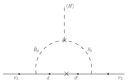
Figure 1: Radiatve Majorana mass generation for active neutrinos via the mixing of singlet-doublet scalar leptoquarks.

With a single leptoquark it is not possible to generate Majorana mass for light neutrinos. Therefore, we need two scalar leptoquarks in the model, which will run in the loop for radiative neutrino mass generation. The singlet-doublet leptoquark mixing, parameterized by $\theta_{\rm LQ}$ in Eq. (5), which depends on the trilinear coupling $\kappa$, is crucial for this purpose, as noted earlier Chua:1999si ; Mahanta:1999xd ; see Fig. 1.

In this singlet-doublet scenario, only $\widetilde{R}_{2}^{1/3}$ and $S_{3}^{1/3}$ together can generate one-loop Majorana mass for active neutrinos, given by Zhang:2021dgl ; Parashar:2022wrd

$$\mathcal{M}_{\nu} = \frac{3\sin 2\theta_{\rm LQ}}{32\pi^{2}}\ln\left(\frac{m_{X_{1}}^{2}}{m_{X_{2}}^{2}}\right)\left(\widetilde{{{\mathcal{Y}_{1}^{L}}}}^{T}\mathcal{M}_{d}{\mathcal{Y}_{2}}+{\mathcal{Y}_{2}}^{T}\mathcal{M}_{d}\widetilde{{\mathcal{Y}_{1}^{L}}}\right).$$ (9)

Here $\widetilde{{\mathcal{Y}_{1}^{L}}}=V\cdot{\mathcal{Y}_{1}^{L}}$ ($V$ being the CKM quark mixing matrix) as we have considered the up-type quarks in their mass basis and $\mathcal{M}_{d}$ is the diagonal mass matrix for down-type quarks. One can obtain the diagonal mass matrix $M_{\nu}^{\rm{diag}}$ (with eigenvalues $m_{\nu_{i}}$, where $i=1,2,3$) for light neutrinos by diagonalizing $\mathcal{M}_{\nu}$ with the usual PMNS lepton mixing matrix $U$ which is parameterized by three mixing angles $\theta_{12},\theta_{13},\theta_{23}$ and three phases i.e., one Dirac phase ($\delta_{\rm{CP}}$) and two Majorana phases ($\alpha,\beta$).

To understand the origin of the Majorana neutrino mass in this scenario, note that one can define a generalized fermion number for leptoquark states as $F=3B+L$  Dorsner:2016wpm . All the SM leptons carry $L=1,B=0$ while the quarks have $L=0,B=1/3$. In our singlet-doublet leptoquark scenario, we can easily deduce from Eq. (2) that $S_{1}$ carries $L=-1,B=-1/3$, while $\widetilde{R}_{2}$ carries $L=-1,B=1/3$. For $S_{1}$ the $F$ number is $-2$ while for $\widetilde{R}_{2}$ it is 0. For the SM Higgs doublet, $B=L=0$. Therefore, within the loop in Fig. 1, lepton number is violated at the trilinear Higgs-leptoquark-leptoquark vertex, which justifies the Majorana mass generation of neutrinos. The trilinear coupling $\kappa$ governs the size of the lepton number breaking, i.e. lepton number symmetry is restored in the limit $\kappa\to 0$.

IV Neutrinoless Double Beta Decay

With Majorana neutrinos, we have the canonical long-range $W_{L}-W_{L}$ contribution to $0\nu\beta\beta$, as shown in Fig. 2(s). In the presence of $S_{1}$ and $\widetilde{R}_{2}$ leptoquarks, we have new long-range contributions to $0\nu\beta\beta$ Hirsch:1996ye mediated by $W_{L}-S_{1}$ exchange, as shown in Figs. 2(a) and (b), as well as from the mixing between $S_{1}$ and $\widetilde{R}_{2}^{1/3}$, as shown in Figs. 2(c) and (d). Diagrams (a) and (c) arise from the ${\mathcal{Y}_{1}^{L}}$ coupling, whereas (b) and (d) arise from the ${\mathcal{Y}_{1}^{R}}$ coupling [cf. Eq. (2)].

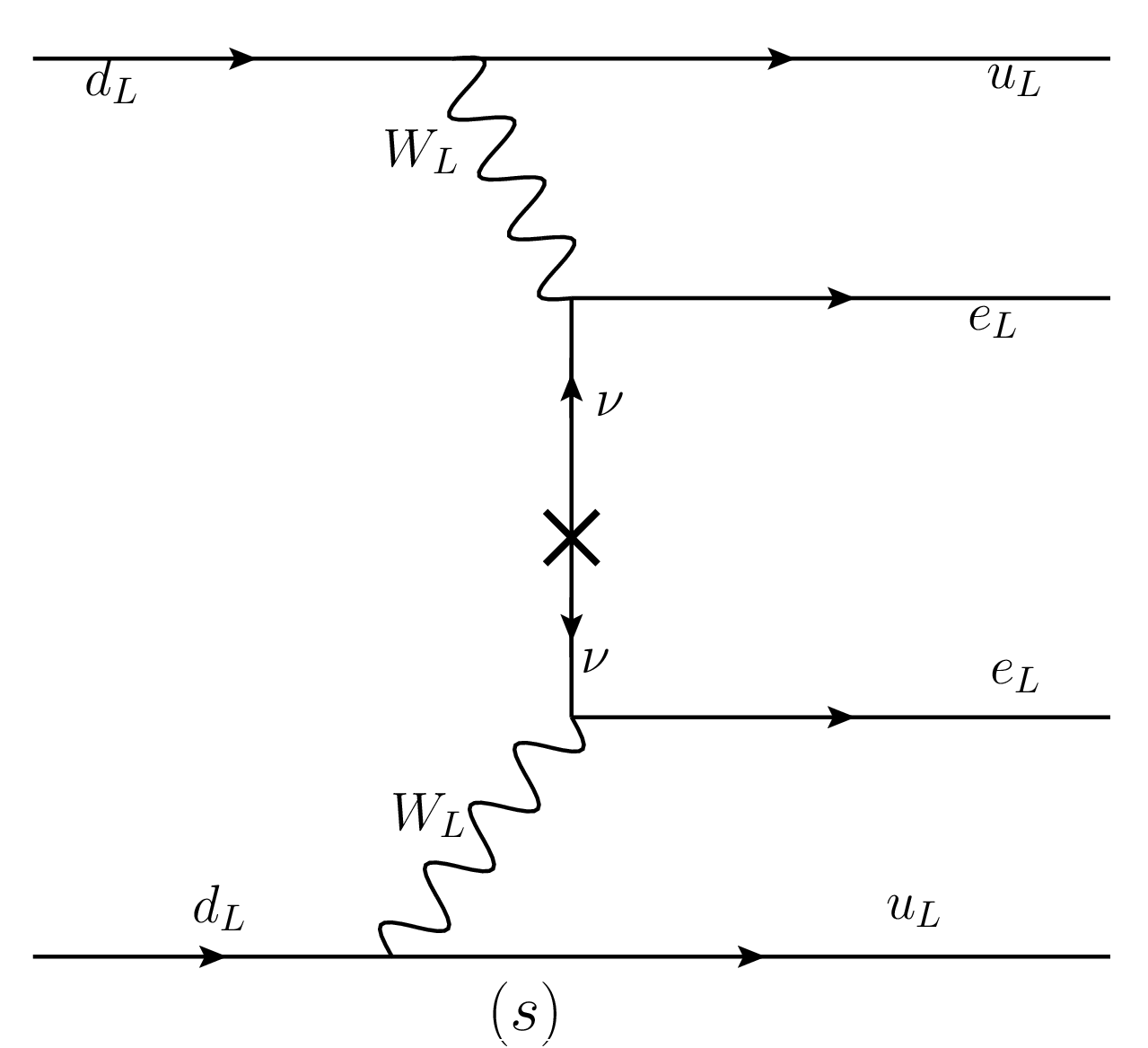
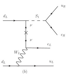
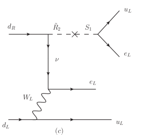
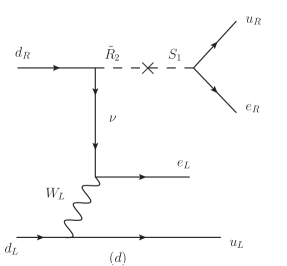
Figure 2: Feynman diagrams for different contributions to the $0\nu\beta\beta$ process in the leptoquark model. The top panel shows the canonical $W_{L}-W_{L}$ mediation for light Majorana neutrinos. The middle panel shows the purely $S_{1}$-mediated diagrams. The bottom panel shows the diagrams mediated by $S_{1}-\widetilde{R}_{2}$ mixing. Diagrams (a) and (c) arise from ${\mathcal{Y}_{1}^{L}}$ coupling, whereas (b) and (d) arise from a combination of ${\mathcal{Y}_{1}^{R}}$ and ${\mathcal{Y}_{2}}$ couplings.

In the standard $W_{L}-W_{L}$ mediation channel, the leptonic and hadronic currents are both connected via the SM gauge boson $W_{L}$, and two electrons of the same helicity ($e_{L}e_{L}$) are emitted, as shown in Fig. 2(s). Here, the dimensionless particle physics parameter can be written as

$$\eta_{\rm std}=\frac{|\sum_{i}U_{ei}^{2}m_{\nu_{i}}|}{m_{e}}\equiv\frac{m_{ee}^{\rm{std}}}{m_{e}},$$ (10)

where $m_{ee}^{\rm{std}}$ represents the effective Majorana mass parameter for the canonical case.

In the leptoquark-mediated channels, depending on whether the ${\mathcal{Y}_{1}^{L}}$ or ${\mathcal{Y}_{1}^{R}}$ couplings are involved, we can have either $e_{L}e_{L}$ or $e_{L}e_{R}$ in the final state, as shown in Fig. 2(a-d). To evaluate these diagrams, we can revert Eq. (6) to write $S_{1}$ and $\widetilde{R}_{2}$ in terms of the mass eigenstates $X_{1}$ and $X_{2}$, and consider the equivalent set of diagrams consisting of $X_{1}-W_{L}$ and $X_{2}-W_{L}$ mediation.

It can be seen from Fig. 2 middle panel that the amplitudes for diagrams (a) and (b) are proportional to the small neutrino mass and inversely proportional to the leptoquark mass squared, which gives an extra suppression relative to the standard mechanism. Hence, the contribution of these diagrams to $0\nu\beta\beta$ can be simply ignored. On the other hand, diagrams (c) and (d), being dependent on the neutrino momentum, give important contribution to $0\nu\beta\beta$ which, depending on the leptoquark mass and couplings, can be dominant over the standard contribution Hirsch:1996ye . The effective operator that generates diagram (c) in Fig. 2 is given by

$$\mathcal{O}_{1}=\left(\frac{G_{F}}{\sqrt{2}}V_{ud}\right)^{2}\left(\overline{u}\gamma_{\mu}P_{L}d\right)\left(\overline{e}\gamma^{\mu}P_{L}\nu\right)\left[\epsilon_{S+P}^{S+P}\left(\overline{u}P_{R}d\right)\left(\overline{\nu}P_{R}e^{c}\right)+\epsilon_{T_{R}}^{T_{R}}\left(\overline{u}\sigma^{\alpha\beta}P_{R}d\right)\left(\overline{\nu}\sigma_{\alpha\beta}P_{R}e^{c}\right)\right],$$ (11)

where the dimensionless parameters $\epsilon_{S+P}^{S+P}$ and $\epsilon_{T_{R}}^{T_{R}}$ can be found as

$$\epsilon_{S+P}^{S+P} = \frac{\cos\theta_{\rm LQ}\sin\theta_{\rm LQ}}{\sqrt{2}\,G_{F}}\left({\mathcal{Y}_{2}}^{*}\right)_{11}\,\left({\mathcal{Y}_{1}^{L}}^{*}\right)_{11}\,\left(\frac{1}{m_{X_{2}}^{2}}-\frac{1}{m_{X_{1}}^{2}}\right),$$ (12)

$$\epsilon_{T_{R}}^{T_{R}} = \frac{1}{4}\,\epsilon_{S+P}^{S+P},$$ (13)

which correspond to the scalar+pseudoscalar and tensor+axial-tensor contributions, respectively. The effective operator that generates diagram (d) in Fig. 2 is given by

$$\mathcal{O}_{2} = \left(\frac{G_{F}}{\sqrt{2}}V_{ud}\right)^{2}\,\epsilon_{V+A}^{V+A}\left(\overline{u}\gamma_{\mu}P_{L}d\right)\left(\overline{e}\gamma^{\mu}P_{L}\nu\right)\,\left(\overline{u}\gamma_{\alpha}P_{R}d\right)\left(\overline{e}\gamma^{\alpha}P_{R}\nu\right),$$ (14)

where the vector+axial-vector term is given by

$$\epsilon_{V+A}^{V+A} = \frac{\cos\theta_{\rm LQ}\sin\theta_{\rm LQ}}{\sqrt{2}\,G_{F}}\left({\mathcal{Y}_{2}}^{*}\right)_{11}\,\left({\mathcal{Y}_{1}^{R}}^{*}\right)_{11}\left(\frac{1}{m_{X_{2}}^{2}}-\frac{1}{m_{X_{1}}^{2}}\right).$$ (15)

With these definitions, the general expression for the $0\nu\beta\beta$ inverse half-life can be written as Kotila:2021xgw

$$\left(T^{0\nu}_{1/2}\right)_{\rm total}^{-1} = \sum_{i,j}G_{ij}\mathrm{Re}\left[X_{i}\,X_{j}^{*}\right]+\sum_{j,k}G^{\prime}_{jk}\mathrm{Re}\left[Y_{j}Y_{k}^{*}\right]+2\sum_{j}G^{\prime\prime}_{i,j}\mathrm{Re}\left[X_{i}\,Y_{j}^{*}\right]$$ (16)

$$= G_{11}\left|X_{1}\right|^{2}+\sum_{\begin{subarray}{c}i,j\end{subarray}}G_{ij}\mathrm{Re}\left[X_{i}\,X_{j}^{*}\right]+\sum_{j,k}G^{\prime}_{jk}\mathrm{Re}\left[Y_{j}Y_{k}^{*}\right]+2\sum_{j}G^{\prime\prime}_{i,j}\mathrm{Re}\left[X_{i}\,Y_{j}^{*}\right],$$

where $G_{ij}$ are the integrated phase space factors (PSFs) and $X_{i}$, $Y_{i}$ are defined in terms of the nuclear matrix elements (NMEs) as

$$X_{1} = \frac{m_{ee}^{\rm std}}{m_{e}}{\mathcal{M}^{LL}_{3,1}},$$ (17)

$$X_{3} = \epsilon_{V+A}^{V+A}\,{\mathcal{M}^{RR}_{3,3}},$$ (18)

$$X_{4} = \epsilon_{V+A}^{V+A}\,{\mathcal{M}^{\prime RR}_{3,4}},$$ (19)

$$Y_{3} = \epsilon_{S+P}^{S+P}{\mathcal{M}^{RR}_{5,3}}+\epsilon_{T_{R}}^{T_{R}}{\mathcal{M}^{RR}_{4,3}}=\epsilon_{S+P}^{S+P}\left({\mathcal{M}^{RR}_{5,3}}+\frac{{\mathcal{M}^{RR}_{4,3}}}{4}\right),$$ (20)

$$Y_{4} = \epsilon_{S+P}^{S+P}{\mathcal{M}^{\prime RR}_{5,4}}+\epsilon_{T_{R}}^{T_{R}}{\mathcal{M}^{\prime RR}_{4,4}}=\epsilon_{S+P}^{S+P}\left({\mathcal{M}^{\prime RR}_{5,4}}+\frac{{\mathcal{M}^{\prime RR}_{4,4}}}{4}\right).$$ (21)

Here $X_{1}$ denotes the SM contribution and the rest are leptoquark contributions. We take the values of NMEs and the corresponding PSFs from Ref. Kotila:2021xgw , obtained by making use of the interacting boson model (IBM2) with isospin restoration for the NMEs Barea:2015kwa and of exact Dirac wave functions for the PSFs Kotila:2012zza . These are tabulated in Tables 1 and 2, respectively. In Eq. (16), the first term is the SM contribution, the second term denotes the $V+A$ contribution, and the third and fourth terms come from both $(S+P)$ and $(T+AT)$ contributions. The first term in Eq. (16) depends on the neutrino masses and PMNS mixing matrix elements, but other terms, in addition, depend on the leptoquark Yukawa couplings, namely, ${\mathcal{Y}_{1}^{L}}$ and ${\mathcal{Y}_{2}}$ in diagram (c), and ${\mathcal{Y}_{1}^{R}}$ and ${\mathcal{Y}_{2}}$ in diagram (d). The tensor contribution was neglected in the literature, as it was considered to have a small contribution Hirsch:1996ye . But we find that in the Fierz transformations (see Appendix A), whenever the (pseudo)scalar contribution is present, the (axial)tensor contribution is also present and it is equally important. In fact, the ratios of the $(T+AT)$-to-$(S+P)$ contributions in our model are given by

$$\left|\frac{\epsilon_{T_{R}}^{T_{R}}\,{\mathcal{M}^{RR}_{4,3}}}{\epsilon_{S+P}^{S+P}\,{\mathcal{M}^{RR}_{5,3}}}\right| = \left|\frac{{\mathcal{M}^{RR}_{4,3}}}{4\,{\mathcal{M}^{RR}_{5,3}}}\right|\simeq 3.95\,,\quad\left|\frac{\epsilon_{T_{R}}^{T_{R}}\,{\mathcal{M}^{\prime RR}_{4,4}}}{\epsilon_{S+P}^{S+P}\,{\mathcal{M}^{\prime RR}_{5,4}}}\right|=\left|\frac{{\mathcal{M}^{\prime RR}_{4,4}}}{4\,{\mathcal{M}^{\prime RR}_{5,4}}}\right|\simeq 2.96,$$ (22)

and hence, cannot be neglected.

${\mathcal{M}^{LL}_{3,1}}$	${\mathcal{M}^{RR}_{3,3}}$	${\mathcal{M}^{\prime RR}_{3,4}}$	${\mathcal{M}^{RR}_{4,3}}$	${\mathcal{M}^{\prime RR}_{4,4}}$	${\mathcal{M}^{RR}_{5,3}}$	${\mathcal{M}^{\prime RR}_{5,4}}$
$-5.36$	$-4.20$	$-2.84$	$-2.85i$	$-4.27i$	$-0.18$	$-0.36$

Table 1: Relevant nuclear matrix elements for the standard and leptoquark contributions, which are computed through IBM2 method for ¹³⁶Xe Kotila:2021xgw .

$G_{11}$	$G_{33}$	$G_{44}$	$G_{13}$	$G_{14}$	$G_{34}$	$G^{\prime}_{33}$	$G^{\prime}_{44}$
14.55	36.48	9.85	$-4.48$	6.13	$-16.01$	36.48	3602.01
$G^{\prime}_{34}$	$G^{\prime\prime}_{13}$	$G^{\prime\prime}_{14}$	$G^{\prime\prime}_{33}$	$G^{\prime\prime}_{44}$	$G^{\prime\prime}_{34}$	$G^{\prime\prime}_{43}$
$-104.55$	$1.02\times 10^{-2}$	155.10	$-4.38\times 10^{-2}$	142.30	$-104.06$	16.06

Table 2: Relevant phase space factors in units of $10^{-15}\,{\rm yr}^{-1}$ for ¹³⁶Xe Kotila:2021xgw .

From Eq. (16), the effective Majorana mass can be extracted as

$$\left(T_{1/2}^{0\nu}\right)_{\rm total}^{-1} = G_{11}\left|X_{1}\right|^{2}+\text{LQ contribution}+\text{SM-LQ interference}$$ (23)

$$\equiv G_{11}\,\left|{\mathcal{M}^{LL}_{3,1}}\right|^{2}\,\frac{\left|m_{ee}^{\rm eff}\right|^{2}}{m^{2}_{e}}\,.$$

The advantage of writing it this way is that when the leptoquark contribution becomes sub-dominant, $m_{ee}^{\rm eff}\to m_{ee}^{\rm std}$. In other words, the deviation of $m_{ee}^{\rm eff}$ from $m_{ee}^{\rm std}$ gives a measure of the leptoquark contribution, including interference with the SM contribution.

Currently, the most stringent constraint on $0\nu\beta\beta$ comes from the KamLAND-Zen experiment using ¹³⁶Xe nuclei, which gives $T_{1/2}^{0\nu}>3.8\times 10^{26}$ yr, which corresponds to $m_{ee}<(28-122)$ meV at 90% CL KamLAND-Zen:2024eml . The uncertainty band in $m_{ee}$ is taking into account multiple NME calculations. The next-generation ton-scale experiment nEXO will reach a sensitivity of $T_{1/2}^{0\nu}>1.35\times 10^{28}$ yrs at 90% CL in 10 years of data taking nEXO:2021ujk . This translates into an upper limit on $m_{ee}<(4.7-20.7)$ meV. The LEGEND-1000 experiment using ⁷⁶Ge isotope will reach a similar design sensitivity of $T_{1/2}^{0\nu}>1.6\times 10^{28}$ yrs at 90% CL LEGEND:2021bnm , which translates into an upper limit on $m_{ee}<(9-21)$ meV. We will use these numbers in our numerical analysis.

V Flavor Observables

In this section, we present the relevant low-energy LFV and LFUV observables which constrain the leptoquark parameter space. There are additional constraints, such as those from perturbative unitarity Lee:1977eg and electroweak $T$-parameter Peskin:1991sw , which however are negligible for our choice of small trilinear coupling $\kappa$, and hence, are not shown here.

V.1 Charged Lepton Sector

Here we consider the cLFV processes $\mu\to e$ conversion, $\ell_{\alpha}\to\ell_{\beta}\gamma$, $\ell_{\alpha}\to\ell_{\beta}\ell_{\gamma}\ell_{\delta}$, and lepton anomalous magnetic moment.

V.1.1 $\mu\rightarrow e$ Conversion in Nuclei

In this model, leptoquark can mediate $\mu\rightarrow\,e$ conversion inside nuclei, i.e. $\mu\,N\rightarrow\,e\,N$. As this process occurs at tree level, it provides one of the most stringent constraints among the flavor observables on the Yukawa couplings involving first and second generation leptons. The conversion ratio is denoted as

$$\left.\mathcal{R}\right|_{\mu\rightarrow\,e}^{N} = \frac{\Gamma^{N}\left(\mu\rightarrow\,e\right)}{\Gamma^{N}_{\rm capture}}\,,$$ (24)

where $N$ denotes a particular nucleus and $\Gamma^{N}_{\rm capture}$ implies the muon capture rate of that nucleus. The low energy effective Lagrangian describing $\mu\,N\rightarrow\,e\,N$ can be written as Kitano:2002mt

$$\mathcal{L}_{\overline{q}q\overline{e}\mu} \supset -\sqrt{2}G_{F}\sum_{q=u,d,s}\sum_{X,Y=L,R}C_{V_{XY}}^{q}\left(\overline{e}\,\gamma^{\mu}\,P_{X}\,\mu\right)\,\left(\overline{q}\,\gamma^{\mu}\,\,P_{Y}q\right)\,+\text{H.c.}$$ (25)

Here, the scalar operators and operators with the gluon field strength tensor are neglected because they are suppressed in this model Plakias:2023esq . The relevant Wilson coefficients are given by

$$C_{V_{LL}^{u}} = \frac{v^{2}}{2}\left({\mathcal{Y}_{1}^{L}}\right)_{12}\left({\mathcal{Y}_{1}^{L}}\right)_{11}^{\ast}\,\left(\frac{\cos^{2}\theta_{\rm LQ}}{m^{2}_{X_{1}}}+\frac{\sin^{2}\theta_{\rm LQ}}{m^{2}_{X_{2}}}\right),$$ (26)

$$C_{V_{LR}^{d}} = -\frac{v^{2}}{2}\frac{\left({\mathcal{Y}_{2}}\right)_{12}\left({\mathcal{Y}_{2}}\right)_{11}^{\ast}}{m^{2}_{\widetilde{R}_{2}^{2/3}}},$$ (27)

$$C_{V_{RR}^{u}} = \frac{v^{2}}{2}\left({\mathcal{Y}_{1}^{R}}\right)_{12}\left({\mathcal{Y}_{1}^{R}}\right)_{11}^{\ast}\left(\frac{\cos^{2}\theta_{\rm LQ}}{m^{2}_{X_{1}}}+\frac{\sin^{2}\theta_{\rm LQ}}{m^{2}_{X_{2}}}\right).$$ (28)

Then the coefficients are combined to form vector and axial vector components that appear in the nucleon EFT Kitano:2002mt :

$$C_{V_{L}}^{p} = \sum_{q}f_{V_{p}}^{q}\,\left(C_{V_{LL}}^{q}+C_{V_{LR}}^{q}\right),\qquad C_{A_{L}}^{p}=\sum_{q}f_{V_{p}}^{q}\,\left(C_{V_{LR}}^{q}-C_{V_{LL}}^{q}\right),$$ (29)

and similarly, for $p\rightarrow\,n$ and $L\rightarrow\,R$. Here, $f_{V_{p}}^{u}=f_{V_{n}}^{d}=2$, $f_{V_{p}}^{d}=f_{V_{n}}^{u}=1$ and $f_{V_{p}}^{s}$ = $f_{V_{n}}^{s}=0$ comes from the valence quark content of nucleons. The effect of the vector part to the conversion ratio is independent of nuclear spin. The axial vector part does depend on the nuclear spin, but the axial vector contribution is much smaller than the vector contribution Davidson:2017nrp . Therefore, we can calculate the spin-independent conversion ratio as

$$\left.\mathcal{R}\right|_{\mu\rightarrow\,e}^{N} = \frac{2\,G_{F}^{2}\,m_{\mu}^{5}}{\Gamma_{\rm capture}^{N}\,\pi^{2}}\,\left(Z\,\alpha_{\rm em}\right)^{3}\left|Z\,F_{p}^{N}(m_{\mu})\,C_{V_{L}}^{p}+(A-Z)\,F_{n}^{N}(m_{\mu})\,C_{V_{L}}^{n}\right|^{2}+L\leftrightarrow R,$$ (30)

where $Z$ and $A$ denote the atomic and mass numbers for the nucleus $N$, respectively. $F_{p}^{N}$ and $F_{n}^{N}$ are nuclear form factors. Currently, the most stringent limit on $\mu\rightarrow\,e$ conversion comes from the SINDRUM experiment using ${}^{197}_{79}$Au nucleus: $\left.\mathcal{R}\right|_{\mu\rightarrow\,e}^{\rm Au}\,<7.0\times 10^{-13}$ SINDRUMII:2006dvw , whereas in the future, the Mu2e experiment at Fermilab Mu2e:2014fns and COMET experiment at J-PARC COMET:2018auw are expected to improve the experimental sensitivity down to $10^{-17}$ level using ${}^{27}_{13}$Al. The muon capture rates and nuclear form factors for these two nuclei are shown in Table 3.

$N$	$\Gamma^{N}_{\rm capture}$ (MeV)	$F_{p}^{N}(m_{\mu})=F_{n}^{N}(m_{\mu})$
Au	$8.7\times 10^{-15}$	0.035
Al	$4.6\times 10^{-16}$	0.53

Table 3: Muon capture rates Suzuki:1987jf and nuclear form factors Kitano:2002mt relevant for $\mu\to e$ conversion in ${}^{197}_{79}$Au and ${}^{27}_{13}$Al.

V.1.2 $\ell_{\alpha}\to\ell_{\beta}\gamma$

As mentioned in Section III, we have leptoquarks with two different generalized fermion numbers, i.e. $F_{S_{1}}=-2\,,\quad F_{\widetilde{R}_{2}}=0$. The interaction of these leptoquarks with the charged lepton can be written as Dorsner:2019itg

$$\mathcal{L}^{|F|=2} \supset \overline{u}_{i}^{c}\left({\mathcal{Y}_{1}^{L}}\right)_{ij}\,P_{L}\,\ell_{j}\,S_{1}^{1/3}+\overline{u}_{i}^{c}\left({\mathcal{Y}_{1}^{R}}\right)_{ij}\,P_{R}\,\ell_{j}\,S_{1}^{1/3}+\text{H.c.},$$ (31)

$$\mathcal{L}^{|F|=0} \supset \overline{d}_{i}\left({\mathcal{Y}_{2}}\right)_{ij}P_{L}\ell_{jL}\,\widetilde{R}_{2}^{2/3}\,.$$ (32)

The $\ell_{\alpha}\to\ell_{\beta}\gamma$ partial decay rate is given by

$$\Gamma\left(l_{\alpha}\rightarrow l_{\beta}\gamma\right) = \frac{\alpha_{\rm em}\,m_{\alpha}^{3}}{4}\left(1-\frac{m_{\beta}^{2}}{m_{\alpha}^{2}}\right)^{3}\left(\left|\sigma_{L}^{\alpha\beta}\right|^{2}+\left|\sigma_{R}^{\alpha\beta}\right|^{2}\right)\,.$$ (33)

Here $\alpha_{\rm em}$ is the fine structure constant, and the $\sigma_{L}$ and $\sigma_{R}$ terms corresponding to the $S_{1}$ and $\widetilde{R}_{2}$ loop contributions are respectively given by

$$\sigma_{L}^{S_{1}} = \frac{i\,N_{c}}{16\pi^{2}m_{S_{1}}^{2}}\sum_{q=u,c,t}\left[\left({\mathcal{Y}_{1}^{L}}\right)_{q\alpha}\left({\mathcal{Y}_{1}^{R}}^{*}\right)_{q\beta}m_{q}\,\mathcal{G}(x_{q})\right.$$ (34)

$$\qquad\qquad\qquad\qquad\left.+\left\{m_{\beta}\,\left({\mathcal{Y}_{1}^{L}}^{*}\right)_{q\beta}\left({\mathcal{Y}_{1}^{L}}\right)_{q\alpha}+m_{\alpha}\,\left({\mathcal{Y}_{1}^{R}}^{*}\right)_{q\beta}\left({\mathcal{Y}_{1}^{R}}\right)_{q\alpha}\right\}\,\mathcal{F}(x_{q})\right],$$

$$\sigma_{R}^{S_{1}} = \frac{i\,N_{c}}{16\pi^{2}m_{S_{1}}^{2}}\sum_{q=u,c,t}\left[\left({\mathcal{Y}_{1}^{L}}^{*}\right)_{q\beta}\left({\mathcal{Y}_{1}^{R}}\right)_{q\alpha}\,m_{q}\,\mathcal{G}(x_{q})\right.$$ (35)

$$\qquad\qquad\qquad\qquad\left.+\left\{m_{\alpha}\,\left({\mathcal{Y}_{1}^{L}}^{*}\right)_{q\beta}\left({\mathcal{Y}_{1}^{L}}\right)_{q\alpha}+m_{\beta}\,\left({\mathcal{Y}_{1}^{R}}^{*}\right)_{q\beta}\left({\mathcal{Y}_{1}^{R}}\right)_{q\alpha}\right\}\,\mathcal{F}(x_{q})\right],$$

$$\sigma_{L}^{\widetilde{R}_{2}} = \frac{i\,N_{c}}{16\pi^{2}\,m^{2}_{\widetilde{R}_{2}^{2/3}}}\sum_{q=d,s,b}\left({\mathcal{Y}_{2}}\right)^{*}_{q\beta}\,\left({\mathcal{Y}_{2}}\right)_{q\alpha}m_{\beta}\,\mathcal{F}(x_{q}),$$ (36)

$$\sigma_{R}^{\widetilde{R}_{2}} = \frac{i\,N_{c}}{16\pi^{2}\,m^{2}_{\widetilde{R}_{2}^{2/3}}}\sum_{q=d,s,b}\left({\mathcal{Y}_{2}}\right)^{*}_{q\beta}\,\left({\mathcal{Y}_{2}}\right)_{q\alpha}m_{\alpha}\,\mathcal{F}(x_{q}).$$ (37)

Here $x_{q}=m_{q}^{2}/m_{\rm LQ}^{2}$, $N_{c}=3$ is the number of colors, and the loop functions $\mathcal{F}(x)$ and $\mathcal{G}(x)$ are given in Appendix B.

For all cLFV processes $\ell_{\alpha}\to\ell_{\beta}\gamma$, the mass of $\ell_{\beta}$ can be neglected with respect to the mass of $\ell_{\alpha}$. In this limit, writing in terms of the leptoquark mass eigenstates, we have

$$\sigma_{L}^{X_{1}} = \frac{i\,N_{c}\cos^{2}\theta_{\rm LQ}}{16\pi^{2}m_{X_{1}}^{2}}\sum_{q=u,c,t}\left[\left({{\mathcal{Y}_{1}^{L}}}\right)_{q\alpha}\left({\mathcal{Y}_{1}^{R}}^{*}\right)_{q\beta}\,m_{q}\,\mathcal{G}(x_{q})+m_{\alpha}\,\left({\mathcal{Y}_{1}^{R}}^{*}\right)_{q\beta}\left({\mathcal{Y}_{1}^{R}}\right)_{q\alpha}\,\mathcal{F}(x_{q})\right],$$ (38)

$$\sigma_{L}^{X_{2}} = \frac{i\,N_{c}\sin^{2}\theta_{\rm LQ}}{16\pi^{2}m_{X_{2}}^{2}}\sum_{q=u,c,t}\left[\left({{\mathcal{Y}_{1}^{L}}}\right)_{q\alpha}\left({\mathcal{Y}_{1}^{R}}^{*}\right)_{q\beta}\,m_{q}\,\mathcal{G}(x_{q})+m_{\alpha}\,\left({\mathcal{Y}_{1}^{R}}^{*}\right)_{q\beta}\left({\mathcal{Y}_{1}^{R}}\right)_{q\alpha}\,\mathcal{F}(x_{q})\right],$$ (39)

$$\sigma_{R}^{X_{1}} = \frac{i\,N_{c}\,\cos^{2}\theta_{\rm LQ}}{16\pi^{2}m_{X_{1}}^{2}}\sum_{q=u,c,t}\left[\left({{\mathcal{Y}_{1}^{L}}}^{*}\right)_{q\beta}\left({\mathcal{Y}_{1}^{R}}\right)_{q\alpha}\,m_{q}\,\mathcal{G}(x_{q})+m_{\alpha}\,\left({{\mathcal{Y}_{1}^{L}}}^{*}\right)_{q\beta}\left({{\mathcal{Y}_{1}^{L}}}\right)_{q\alpha}\,\mathcal{F}(x_{q})\right],$$ (40)

$$\sigma_{R}^{X_{2}} = \frac{i\,N_{c}\,\sin^{2}\theta_{\rm LQ}}{16\pi^{2}m_{X_{2}}^{2}}\sum_{q=u,c,t}\left[\left({{\mathcal{Y}_{1}^{L}}}^{*}\right)_{q\beta}\left({\mathcal{Y}_{1}^{R}}\right)_{q\alpha}\,m_{q}\,\mathcal{G}(x_{q})+m_{\alpha}\,\left({{\mathcal{Y}_{1}^{L}}}^{*}\right)_{q\beta}\left({{\mathcal{Y}_{1}^{L}}}\right)_{q\alpha}\,\mathcal{F}(x_{q})\right].$$ (41)

Then the total $\sigma$ (for a given $\alpha\beta$ combination) can be written as

$$\sigma_{L} = \sigma_{L}^{X_{1}}+\sigma_{L}^{X_{2}},\qquad\sigma_{R}=\sigma_{R}^{X_{1}}+\sigma_{R}^{X_{2}}\,.$$ (42)

The cLFV decay branching ratios (BRs) can be written as

$${\rm BR}\left(\ell_{\alpha}\rightarrow\ell_{\beta}\gamma\right) = \frac{\alpha_{\rm em}\,m_{\alpha}^{3}}{4\,\Gamma_{\alpha}}\left(\left|\sigma_{L}^{\alpha\beta}\right|^{2}+\left|\sigma_{R}^{\alpha\beta}\right|^{2}\right)\,.$$ (43)

Here $\Gamma_{\alpha}$ is the total decay width for lepton flavor $\alpha$, which is $2.996\times 10^{-19}~{}\rm GeV$ for $\mu$ and $2.267\times 10^{-12}~{}\rm GeV$ for $\tau$.

These theoretical predictions for the LFV BRs are to be compared with the current experimental upper limits:

${\rm BR}\left(\mu\rightarrow\,e\gamma\right)<3.1\times 10^{-13}$	MEG-II MEGII:2023ltw ,
${\rm BR}\left(\tau\rightarrow\,\mu\,\gamma\right)<4.2\times 10^{-8}$	Belle Belle:2021ysv ,
${\rm BR}\left(\tau\rightarrow\,e\,\gamma\right)<3.3\times 10^{-8}$	BaBar BaBar:2009hkt .

Belle-II is expected to improve the tau LFV limits by a factor of few Belle-II:2022cgf .

V.1.3 Lepton $g-2$

The same one-loop diagrams that contribute to $\ell_{\alpha}\to\ell_{\beta}\gamma$ also give rise to the anomalous magnetic moment of $\ell_{\alpha}$ for $\alpha=\beta$. The leptoquark contribution can thus be written as

$$\Delta a_{\alpha}=i\,m_{\alpha}\left(\sigma_{L}^{\alpha}+\sigma_{R}^{\beta}\right),$$ (44)

where

$$\sigma_{L} = \frac{i\,N_{c}m_{\alpha}}{16\pi^{2}}\left(\frac{\cos^{2}\theta_{\rm LQ}}{m_{X_{1}}^{2}}+\frac{\sin^{2}\theta_{\rm LQ}}{m_{X_{2}}^{2}}\right)\sum_{q=u,c,t}\left[\left({\mathcal{Y}_{1}^{L}}\right)_{q\alpha}\left({\mathcal{Y}_{1}^{R}}^{*}\right)_{q\alpha}\,m_{q}\,\mathcal{G}(x_{q})\right.$$ (45)

$$\qquad\qquad\qquad\qquad\qquad\qquad\qquad\qquad\left.+m_{\alpha}\,\left(\left|\left({\mathcal{Y}_{1}^{R}}\right)_{q\alpha}\right|^{2}+\left|\left({\mathcal{Y}_{1}^{L}}\right)_{q\alpha}\right|^{2}\right)\,\mathcal{F}(x_{q})\right],$$

$$\sigma_{R} = \frac{i\,N_{c}m_{\alpha}}{16\pi^{2}}\left(\frac{\cos^{2}\theta_{\rm LQ}}{m_{X_{1}}^{2}}+\frac{\sin^{2}\theta_{\rm LQ}}{m_{X_{2}}^{2}}\right)\sum_{q=u,c,t}\left[\left({{\mathcal{Y}_{1}^{L}}}^{*}\right)_{q\alpha}\left({\mathcal{Y}_{1}^{R}}\right)_{q\alpha}\,m_{q}\,\mathcal{G}(x_{q})\right.$$ (46)

$$\qquad\qquad\qquad\qquad\qquad\qquad\qquad\qquad\left.+m_{\alpha}\,\left(\left|\left({\mathcal{Y}_{1}^{R}}\right)_{q\alpha}\right|^{2}+\left|\left({\mathcal{Y}_{1}^{L}}\right)_{q\alpha}\right|^{2}\right)\,\mathcal{F}(x_{q})\right]\,.$$

For muon $(g-2)$, the old BNL experiment reported a $3.7\sigma$ discrepancy with respect to the SM prediction Muong-2:2006rrc . The BNL result was recently confirmed by the Fermilab Muon $g-2$ collaboration Muong-2:2023cdq , which increased the discrepancy to $5\sigma$ level, if we use the 2020 world average of the SM prediction Aoyama:2020ynm . However, the BMW lattice result Borsanyi:2020mff disagrees with the world average Aoyama:2020ynm . Other lattice calculations now seem to agree with the BMW result at least in the ‘intermediate distance regime’ gm2theory , but a more thorough analysis is ongoing. In this murky situation, we choose to use the BMW result, which gives a $1.5\sigma$ deviation from the experimental result: $\Delta a_{\mu}=\left(1.07\pm 0.70\right)\times 10^{-9}$ Wittig:2023pcl .

The situation for electron $(g-2)$ is no better. Although the experimental value of $a_{e}$ has been measured very precisely Fan:2022eto , the SM prediction Aoyama:2019ryr relies on the measurement of the fine-structure constant, and currently there is $>5\sigma$ discrepancy between the results derived using two different measurements based on Rb Morel:2020dww and Cs Parker:2018vye atoms. Here we will use both Rb and Cs results in our analysis: $\Delta a_{e}({\rm Rb})=(4.4\pm 3.0)\times 10^{-13}$ Morel:2020dww and $\Delta a_{e}({\rm Cs})=(-8.8\pm 3.6)\times 10^{-13}$ Parker:2018vye .

V.1.4 $\ell_{\alpha}\to\ell_{\beta}\ell_{\gamma}\ell_{\delta}$

The four-lepton LFV amplitude is mediated by box diagrams involving leptoquarks and quarks. The amplitudes of there diagrams scale as $\mathcal{Y}^{4}/m_{\rm LQ}^{2}$, where $\mathcal{Y}$ is the relevant leptoquark coupling. The bounds coming from the box diagrams turn out to be subdominant to those from $\ell_{\alpha}\to\ell_{\beta}\gamma$ Davidson:1993qk . However, the photon penguin contribution to $\ell_{\alpha}\to\ell_{\beta}\ell_{\gamma}\ell_{\delta}$ can be dominant over the $\ell_{\alpha}\to\ell_{\beta}\gamma$ contribution for unitary coupling matrices Gabrielli:2000te . The expressions for the relevant branching ratios can be found in Ref. Gabrielli:2000te . Since the $\mu\to e$ conversion in nuclei gives the strongest cLFV bound, we do not show the results for $\mu\to 3e$ type processes here.

V.2 Rare Meson Decays

Here we discuss the leptoquark contributions to the (semi)leptonic rare decays of $B$ and $K$ mesons. We will consider the neutral-current $B$ decays involving $b\to s\ell^{+}\ell^{-}$ and charged-current $B$ decays involving $b\to c\ell\overline{\nu}$, in particular the LFUV observables parameterized in terms of the ratios of BRs,

$$R_{D^{(*)}} =\frac{{\rm BR}(\overline{B}\to D^{(*)}\tau\overline{\nu})}{{\rm BR}(\overline{B}\to D^{(*)}\ell\overline{\nu})}\quad{\rm with}~{}\ell=e,\mu,$$ (47)

$$R_{K} =\frac{{\rm BR}(B^{+}\to K^{+}\mu^{+}\mu^{-})}{{\rm BR}(B^{+}\to K^{+}e^{+}e^{-})},$$ (48)

$$R_{K^{*}} =\frac{{\rm BR}(B^{0}\to K^{*0}\mu^{+}\mu^{-})}{{\rm BR}(B^{0}\to K^{*0}e^{+}e^{-})},$$ (49)

which are theoretically clean observables with strongly suppressed hadronic and CKM-angle uncertainties. We also consider other rare decays such as $B\to K\nu\overline{\nu}$, $K^{+}\to\pi^{+}\nu\overline{\nu}$, and the rare kaon decays $K_{L}\to\mu^{\pm}e^{\mp}$ and $K^{+}\to\pi^{+}\mu^{\pm}e^{\mp}$.

V.2.1 $R_{K}\text{ and }R_{K^{*}}$

In this model, the $\widetilde{R}_{2}$ contributes to $R_{K}$ and $R_{K^{*}}$, with the effective Hamiltonian written as

$$\mathcal{H}_{\rm eff} = \frac{\left({\mathcal{Y}_{2}}\right)_{s\ell}\left({\mathcal{Y}_{2}}^{*}\right)_{b\ell}}{m^{2}_{\widetilde{R}_{2}}}\left(\overline{s}P_{L}\ell\right)\,\left(\overline{\ell}P_{R}\,b\right)$$ (50)

$$= \frac{\left({\mathcal{Y}_{2}}\right)_{s\ell}\left({\mathcal{Y}_{2}}^{*}\right)_{b\ell}}{2\,m^{2}_{\widetilde{R}_{2}}}\left(\overline{s}\gamma_{\mu}P_{R}b\right)\,\left(\overline{\ell}\gamma^{\mu}\,P_{L}\,\ell\right)$$

$$\equiv \frac{4G_{F}}{\sqrt{2}}V_{tb}\,V^{*}_{ts}\left(\delta C^{\prime}_{9}\,{\cal O}^{\prime}_{9}+\delta C^{\prime}_{10}\,{\cal O}^{\prime}_{10}\right)\,,$$

where the operators ${\cal O}^{\prime}_{9}$ and ${\cal O}^{\prime}_{10}$ are defined as

$${\cal O}^{\prime}_{9} = \frac{\alpha_{\rm em}}{4\pi}\left(\overline{s}\gamma_{\mu}P_{R}b\right)\,\left(\overline{\ell}\gamma^{\mu}\,\ell\right),$$ (51)

$${\cal O}^{\prime}_{10} = \frac{\alpha_{\rm em}}{4\pi}\left(\overline{s}\gamma_{\mu}P_{R}b\right)\,\left(\overline{\ell}\gamma^{\mu}\,\gamma^{5}\,\ell\right),$$ (52)

and the coefficients are identified as

$$\delta C^{\prime}_{9} = -\delta C^{\prime}_{10}=\frac{\pi\,v^{2}}{\alpha_{\rm em}\,V_{tb}\,V^{*}_{ts}}\,\frac{\left({\mathcal{Y}_{2}}\right)_{s\ell}\left({\mathcal{Y}_{2}}^{*}\right)_{b\ell}}{4\,m^{2}_{\widetilde{R}_{2}}}.$$ (53)

The LHCb experiment recently presented new measurements of the $R_{K^{(*)}}$ ratios which turned out to be compatible with the SM LHCb:2022qnv ; LHCb:2022vje . From a recent global analysis using all available $b\to s\ell^{+}\ell^{-}$ data Hurth:2023jwr , it was found that the primed operators ${\cal O}^{\prime}_{9}$ and ${\cal O}^{\prime}_{10}$ (with right chiral quark currents) are loosely constrained with the best-fit values

$$\delta C^{\prime}_{9} = 0.06\pm 0.31,\quad\quad\delta C^{\prime}_{10}=-0.05\pm 0.19.$$ (54)

Therefore, $R_{K^{(*)}}$ does not impose a stringent constraint on the leptoquark model parameter space.

V.2.2 $R_{D}\text{ and }R_{D^{*}}$

Both $S_{1}$ and $\widetilde{R}_{2}$ leptoquarks contribute to $R_{D^{(*)}}$. The effective Hamiltonian can be written as

$$\mathcal{H}_{\rm eff} = \frac{4\,G_{F}}{\sqrt{2}}V_{cb}\left[\left(\delta_{\ell\tau}+C_{V_{L}}\right)\,{\cal O}_{V_{L}}+C_{S_{L}}\,{\cal O}_{S_{L}}+C_{T_{L}}\,{\cal O}_{T_{L}}\right],$$ (55)

where the operators are defined as

$${\cal O}_{V_{L}} = \left(\overline{c}\gamma^{\mu}P_{L}b\right)\left(\overline{\ell}\gamma_{\mu}P_{L}\nu\right),$$ (56)

$${\cal O}_{S_{L}} = \left(\overline{c}P_{L}\,b\right)\left(\overline{\ell}\,P_{L}\,\nu\right),$$ (57)

$${\cal O}_{T_{L}} = \left(\overline{c}\,\sigma^{\mu\nu}\,P_{L}\,b\right)\left(\overline{\ell}\,\sigma_{\mu\nu}\,P_{L}\,\nu\right),$$ (58)

and the $\delta_{\ell\tau}$ term denotes the SM-dominant contribution for $b\rightarrow c\tau^{-}\overline{\nu}$. The Wilson coefficients can be found as

$$C_{V_{L}} = \frac{v^{2}}{V_{cb}}\,\frac{\left({\mathcal{Y}_{1}^{L}}^{*}\right)_{c\ell}\left(\widetilde{{\mathcal{Y}_{1}^{L}}}\right)_{b\ell}}{8}\,\left(\frac{\cos^{2}\theta_{\rm LQ}}{m_{X_{1}}^{2}}+\frac{\sin^{2}\theta_{\rm LQ}}{m_{X_{2}}^{2}}\right),$$ (59)

$$C_{S_{L}} = \frac{v^{2}}{V_{cb}}\,\frac{\left({\mathcal{Y}_{1}^{R}}^{*}\right)_{c\ell}\left(\widetilde{{\mathcal{Y}_{1}^{L}}}\right)_{b\ell}}{8}\,\left(\frac{\cos^{2}\theta_{\rm LQ}}{m_{X_{1}}^{2}}+\frac{\sin^{2}\theta_{\rm LQ}}{m_{X_{2}}^{2}}\right),$$ (60)

$$C_{T_{L}} = -\frac{C_{S_{L}}}{4}.$$ (61)

These Wilson coefficients are extracted at $\mu=m_{\rm LQ}$. To compare with the experimental observables, we need to run them down to $\mu=m_{b}=4.18$ GeV using the renormalization group equations, i.e.

$$C_{i}(\mu=m_{b})\,=\,\Omega_{N}(\mu,m_{\mathrm{LQ}})\;C_{i}(m_{\mathrm{LQ}})\,,$$ (62)

where at the lowest order (leading logarithm), the evolution operator is given by Chetyrkin:1997dh ; Gracey:2000am ; Dorsner:2013tla ; Hiller:2016kry

$$\Omega_{N}(\mu,M_{\mathrm{LQ}})\,=\,\left(\frac{\alpha_{s}^{(5)}(m_{b})}{\alpha^{(5)}_{s}(m_{t})}\right)^{-\gamma^{J}_{1}/\beta_{1}^{(5)}}\;\left(\frac{\alpha_{s}^{(6)}(m_{t})}{\alpha^{(6)}_{s}(m_{\mathrm{LQ}})}\right)^{-\gamma^{J}_{1}/\beta_{1}^{(6)}},$$ (63)

with QCD running $\beta$-function, $\beta_{1}^{(n_{f})}=(2n_{f}-33)/6$, where $n_{f}$ is the relevant number of quark flavors at the hadronic scale. The anomalous dimensions for the currents are

$$\gamma_{1}^{V}=0\,,\qquad\qquad\gamma_{1}^{S}=2\,,\qquad\qquad\gamma_{1}^{T}=-2/3\,.$$ (64)

Note that the vector currents are not affected, while the scalar and tensor currents renormalize multiplicatively. With the given effective operators, we can express the ratio of $R_{D}\,(R_{D^{*}})$ to the SM prediction Iguro:2024hyk :

$$r_{D}=\frac{R_{D}}{R_{D}^{\rm SM}} \approx \left|1+C_{V_{L}}\right|^{2}+1.01\,\left|C_{S_{L}}\right|^{2}+0.84\,\left|C_{T_{L}}\right|^{2}+1.49\,\,{\rm Re}\left[(1+C_{V_{L}})\,C_{S_{L}}^{*}\right]$$ (65)

$$\qquad+1.08\,\,\rm Re\left[(1+C_{V_{L}})\,C_{T_{L}}^{*}\right],$$

$$r_{D^{*}}=\frac{R_{D^{*}}}{R_{D^{*}}^{\rm SM}} \approx \left|1+C_{V_{L}}\right|^{2}+0.04\left|C_{S_{L}}\right|^{2}+16.07\left|C_{T_{L}}\right|^{2}$$ (66)

$$\qquad-0.11\,\,\rm Re\left[(1+C_{V_{L}})\,C_{S_{L}}^{*}\right]-5.17\,\,{\rm Re}\left[(1+C_{V_{L}})\,C_{T_{L}}^{*}\right].$$

Using a recent global fit to the experimental results, Ref. Iguro:2024hyk found a $4.3\sigma$ deviation from the SM prediction:

$$r_{D} = 1.186\pm 0.072,\quad\quad r_{D^{*}}=1.149\pm 0.04.$$ (67)

Treating this $R_{D^{(*)}}$ anomaly at the face value, we will analyze the parameter space which can successfully fit this anomaly. Given the volatile situation with flavor anomalies, we will also present our results for a hypothetical case where this anomaly disappears with more data in the future, i.e. both $R_{D}$ and $R_{D^{*}}$ are consistent with the SM predictions.

V.2.3 $B\to K\,\nu\,\overline{\nu}$

Leptoquarks can also induce rare semileptonic $B$ decays like $B^{+}\rightarrow K^{+}\,\nu\,\overline{\nu}$ and $B^{0}\rightarrow{K^{*}}^{0}\,\nu\,\overline{\nu}$, governed by $(\overline{q}\,q\,\overline{\nu}\nu)$ effective interactions. The SM predictions for these decays are ${\rm BR}\left(B^{+}\rightarrow\,K^{+}\,\nu\,\overline{\nu}\right)\,=\,(4.65\pm 0.62)\times 10^{-6}$ and ${\rm BR}\left(B^{0}\rightarrow\,{K^{*}}^{0}\,\nu\,\overline{\nu}\right)\,=\,(10.13\pm 0.92)\times 10^{-6}$ Buras:2022wpw . Belle-II recently reported the first observation of $B^{+}\rightarrow K^{+}\,\nu\,\overline{\nu}$ decay Belle-II:2023esi . Using the weighted average of BABAR, Belle and Belle-II data, Ref. Buras:2024ewl quoted an experimental value for ${\rm BR}\left(B^{+}\rightarrow\,K^{+}\,\nu\,\overline{\nu}\right)_{\rm exp}=(1.3\pm 0.4)\times\,10^{-5}$. As for $B^{0}\rightarrow\,{K^{*}}^{0}\,\nu\,\overline{\nu}$, the current experimental upper limit is ${\rm BR}\left(B^{0}\rightarrow\,{K^{*}}^{0}\,\nu\,\overline{\nu}\right)<2.7\times\,10^{-5}$ at 90% CL by the Belle collaboration Belle:2017oht . The constraints on new physics (NP) contributions are expressed in terms of the ratios $R^{\nu\nu}_{K^{(*)}}$, defined as

$$R^{\nu\nu}_{K^{(*)}}=\frac{{\rm BR}^{\rm SM+NP}\left(B\rightarrow K^{(*)}\nu\overline{\nu}\right)}{{\rm BR}^{\rm SM}\left(B\rightarrow K^{(*)}\nu\overline{\nu}\right)}.$$ (68)

From the recent Belle-II measurement Belle-II:2023esi , we get $R_{K}^{\nu\nu}=(2.8\pm 0.94)$ and from the Belle upper limit Belle:2017oht , we get $R_{K^{*}}^{\nu\nu}<2.7$.

The relevant effective Hamiltonian governing these decays can be written as

$$\mathcal{H}_{\rm eff} = \frac{4\,G_{F}}{\sqrt{2}}V_{tb}\,V^{*}_{ts}\left(C^{ij}_{L}\,\mathcal{O}^{ij}_{L}+C^{ij}_{R}\mathcal{O}^{ij}_{R}\right),$$ (69)

where the operators are defined as

$$\mathcal{O}^{ij}_{L} = \frac{\alpha_{\rm em}}{4\pi}\left(\overline{d}\gamma^{\mu}P_{L}s\right)\left(\overline{\nu}_{i}\gamma_{\mu}(1-\gamma_{5})\nu_{j}\right),$$ (70)

$$\mathcal{O}^{ij}_{R} = -\frac{\alpha_{\rm em}}{4\pi}\left(\overline{d}\gamma^{\mu}P_{R}s\right)\left(\overline{\nu}_{i}\gamma_{\mu}(1-\gamma_{5})\nu_{j}\right).$$ (71)

The corresponding Wilson coefficients are given as

$$C^{ij}_{L} = C_{\rm SM}\delta^{ij}+\delta C_{L}^{ij}$$ (72)

$$= C_{\rm SM}\delta^{ij}+\frac{\pi\,v^{2}}{4\alpha_{\rm em}\,V_{tb}\,V^{*}_{ts}}\,\left(\frac{\cos^{2}\theta}{m_{X_{1}}^{2}}+\frac{\sin^{2}\theta}{m_{X_{2}}^{2}}\right)\,\left(\widetilde{{\mathcal{Y}_{1}^{L}}}\right)_{2j}\,\left(\widetilde{{\mathcal{Y}_{1}^{L}}^{*}}\right)_{3i},$$

$$C^{ij}_{R} = \delta C_{R}^{ij}=-\frac{\pi\,v^{2}}{4\alpha_{\rm em}\,V_{tb}\,V^{*}_{ts}}\,\left(\frac{\sin^{2}\theta}{m_{X_{1}}^{2}}+\frac{\cos^{2}\theta}{m_{X_{2}}^{2}}\right)\,\left({\mathcal{Y}_{2}}\right)_{2j}\,\left({\mathcal{Y}_{2}}^{*}\right)_{3i}.$$ (73)

As the experiments cannot tag the neutrino flavor, we need to sum over all possible flavor combinations while calculating the ratio of branching fractions in Eq. (68). The ratios can be expressed as Browder:2021hbl ; He:2023bnk

$$R_{K}^{\nu\nu} = \frac{1}{3\left|C_{\rm SM}\right|^{2}}\sum_{i,j}\left|C_{L}^{ij}+C_{R}^{ij}\right|^{2},$$ (74)

$$R_{K^{*}}^{\nu\nu} = \frac{1}{3\left|C_{\rm SM}\right|^{2}}\sum_{i,j}\left|C_{L}^{ij}+C_{R}^{ij}\right|^{2}-\frac{2}{3\left|C_{\rm SM}\right|^{2}}\left(1+\eta\right)\sum_{i,j}\,{\rm Re}\,\left[C_{L}^{ij}\,C_{R}^{*ij}\right]$$ (75)

The numerical value of $\eta$ was found to be $0.33\pm 0.09$ using the Light Cone Sum Rule (LCSR) method Gubernari:2018wyi .

V.2.4 $K\to\pi\,\nu\,\overline{\nu}$

Apart from $B$ meson decays, leptoquark models are also constrained from the rare $K$ meson decays. One such example is $K^{+}\rightarrow\,\pi\nu\,\overline{\nu}$ which gets tree-level contribution from the scalar leptoquarks Bobeth:2017ecx ; Fajfer:2018bfj ; Mandal:2019gff ; Buras:2024ewl . The experimentally determined value is ${\rm BR}\left(K^{+}\rightarrow\pi^{+}\nu\overline{\nu}\right)_{\rm exp}=\left(10.6^{+4.1}_{-3.5}\times 10^{-11}\right)$ by NA62 NA62:2021zjw which is consistent with the SM prediction ${\rm BR}\left(K^{+}\rightarrow\pi^{+}\nu\overline{\nu}\right)_{\rm SM}=(7.73\pm 0.61)\times 10^{-11}$ Brod:2021hsj . Theoretically, the BR of $K^{+}\rightarrow\pi^{+}\nu\,\nu$ can be written as  Bobeth:2016llm ; Bobeth:2017ecx

$${\rm BR}\left(K^{+}\rightarrow\pi^{+}\nu\nu\right) = \kappa_{+}\frac{\left(1+\Delta_{\rm em}\right)}{3\,\lambda^{10}}\sum_{i,j=e,\mu,\tau}\left[{\rm Im}^{2}\left(\lambda_{t}^{sd}\,X_{t}^{ij}\right)+{\rm Re}^{2}\left(\lambda_{c}^{sd}\,X_{c}^{ii}+\lambda_{t}^{sd}\,X_{t}^{ij}\right)\right],$$ (76)

where $i,j$ denote the flavors of the emitted neutrinos, $\lambda=0.225$ is the Wolfenstein parameter of the CKM matrix, $\Delta_{\rm em}=-0.003$, $\kappa_{+}=0.52\times 10^{-10}\left(\frac{\lambda}{0.225}\right)$ and $\lambda^{sd}_{q}=V_{qs}\,V_{qd}^{\ast}$, where $q$ is the quark flavor. The short-distance contribution $X$ is defined as $X_{q}^{ij}=X_{\rm SM}(x_{q})\delta_{ij}+X_{\rm LQ}^{ij}$. Here $x_{q}=m_{q}^{2}/m_{\rm LQ}^{2}$. In the SM, the dominant contribution to the branching ratio comes from the top quark and the corresponding $X_{\rm SM}(m_{t})=1.481\pm 0.009$ Bobeth:2016llm . NP contributions in our leptoquark model can be written as

$$X_{\rm LQ}^{ij}=-\frac{\sin^{2}\theta_{w}\,\pi v^{2}\,}{\alpha_{\rm em}}\,\frac{\left(C_{L}^{ij}+C_{R}^{ij}\right)}{\lambda_{t}^{sd}},$$ (77)

where $\theta_{w}$ is the weak mixing angle, and

$$C_{L}^{ij} = \frac{1}{2}\,\left(\widetilde{{\mathcal{Y}_{1}^{L}}}\right)_{2i}\left(\widetilde{{\mathcal{Y}_{1}^{L}}}\right)_{1j}\,\left(\frac{\cos^{2}\theta_{\rm LQ}}{m_{X_{1}}^{2}}+\frac{\sin^{2}\theta_{\rm LQ}}{m_{X_{2}}^{2}}\right),$$ (78)

$$C_{R}^{ij} = \frac{1}{2}\left({\mathcal{Y}_{2}}\right)_{2i}\left({\mathcal{Y}_{2}}\right)_{1j}\,\left(\frac{\sin^{2}\theta_{\rm LQ}}{m_{X_{1}}^{2}}+\frac{\cos^{2}\theta_{\rm LQ}}{m_{X_{2}}^{2}}\right).$$ (79)

We can also consider the analogous decay of the neutral kaon, $K_{L}\to\pi^{0}\nu\overline{\nu}$. However, this has not been observed yet, and there only exists an upper bound on ${\rm BR}(K_{L}\to\pi^{0}\nu\overline{\nu})_{\rm exp}<4.9\times 10^{-9}$ from KOTO KOTO:2020prk . This is more than two orders of magnitude larger than the SM prediction: ${\rm BR}(K_{L}\to\pi^{0}\nu\overline{\nu})_{\rm SM}=(2.94\pm 0.15)\times 10^{-11}$ Buras:2021nns . Therefore, this process cannot put any meaningful constraint on the NP scenario at the moment.

V.2.5 $K_{L}\to\mu^{\pm}e^{\mp}$ and $K^{+}\to\pi^{+}\mu^{\pm}e^{\mp}$

The effective Hamiltonian for these purely leptonic decays of the pseudoscalar meson $P\rightarrow\,\ell_{i}\,\ell_{j}$ and $P\rightarrow\,P^{\prime}\,\ell_{i}\,\ell_{j}$ can be written as

$$\mathcal{H}_{\rm LEFT}=\sqrt{2}\,G_{F}\sum_{I\in\left\{V,S,T\right\}}C_{I_{XY}}\,\mathcal{O}_{I_{XY}},$$ (80)

where $X,Y\in\{L,R\}$. The relevant operator for $K_{L}\rightarrow\,\ell^{-}_{i}\,\ell^{+}_{j}$ and $K^{+}\rightarrow\,\pi^{+}\,\ell^{-}_{i}\,\ell^{+}_{j}$ is $\mathcal{O}_{V_{LR}}^{ij21}=\left(\overline{\ell}_{i}\gamma^{\mu}\,P_{L}\,\ell_{j}\right)\,\left(\overline{s}\gamma_{\mu}\,P_{R}\,d\right)$ and the corresponding Wilson coefficients are denoted as

$$C_{V_{LR}}^{ij21}=\frac{\left({\mathcal{Y}_{2}}\right)_{1i}\left({\mathcal{Y}_{2}}\right)_{2j}^{\ast}}{\sqrt{2}\,G_{F}\,m^{2}_{\widetilde{R}_{2}^{2/3}}}.$$ (81)

Here $1,2$ correspond to the first (down) and second (strange) generation quarks. The branching ratio of $K_{L}\rightarrow\ell_{i}^{-}\ell_{j}^{+}$ can be computed as Plakias:2023esq

$${\rm BR}\left(K_{L}\rightarrow\ell_{i}^{-}\ell_{j}^{+}\right) = \tau_{K}\frac{f_{K}^{2}\,m_{K}\,m^{2}_{\ell}}{128\,\pi\,v^{4}}\left(1-\frac{m_{\ell}^{2}}{m_{K}^{2}}\right)^{2}\left\{\left|C_{VA}^{ij}\right|^{2}+\left|C_{AA}^{ij}\right|^{2}\right\},$$ (82)

where $m_{K}$ is the kaon mass, $\tau_{K}$ is its lifetime, and $f_{K}$ is the kaon decay constant. The Wilson coefficients in Eq. (82) are given by

$$C_{VA}^{ij} = \frac{1}{\sqrt{2}}\left(C_{VL}^{ij21}+C_{VL}^{ji12}\right),\qquad C_{AA}^{ij}=-C_{VA}^{ij}.$$ (83)

Similarly, the branching ratio for $K^{+}\rightarrow\,\pi^{+}\,\ell_{i}\,\ell_{j}$ can be written as Plakias:2023esq

$${\rm BR}\left(K^{+}\rightarrow\,\pi^{+}\,\ell_{i}\,\ell_{j}\right) = a_{VV}\left|C^{ij}_{VV}\right|^{2}+a_{AV}\,\left|C^{ij}_{AV}\right|^{2}$$ (84)

where $a_{VV}\simeq a_{AV}\simeq 0.157$ are kaon form factors in the limit where the light lepton mass is neglected. The Wilson coefficients are computes as

$$C^{ij}_{VV} = C^{ij}_{V_{LR}}\,,\qquad C^{ij}_{AV}=-C_{V_{LR}}^{ij}.$$ (85)

These BRs are subjected to stringent experimental limits: ${\rm BR}\left(K_{L}\rightarrow\mu^{\pm}e^{\mp}\right)<4.7\times 10^{-12}$ BNL:1998apv and ${\rm BR}\left(K^{+}\rightarrow\,\pi^{+}\,\mu^{+}\,e^{-}\right)<1.3\times 10^{-11}$ Sher:2005sp at 90% CL.

VI Numerical Analysis

In this section, we use all the abovementioned constraints and perform a multidimensional scan over all the leptoquark parameters to carve out the allowed parameter space.

VI.1 Parametrization of the Yukawa Coupling Matrix

In the canonical seesaw mechanism, the Yukawa couplings can be expressed in terms of the PMNS mixing matrix elements and light neutrino masses using the Casas-Ibarra (CI) parametrization Casas:2001sr . However, in the leptoquark scenario with multiple Yukawa couplings, the standard CI approach does not work. However, one can use a similar approach to parameterize one Yukawa coupling in terms of the others, PMNS matrix elements and neutrino masses Dolan:2018qpy , as follows:

$${\mathcal{Y}_{2}}=\frac{1}{\mathbf{C}_{1}}\,\mathcal{M}_{d}^{-1}\,\left(\widetilde{{\mathcal{Y}_{1}^{L}}}^{T}\right)^{-1}\,U^{*}\,\sqrt{\mathcal{M}_{\nu}^{\rm diag}}\,\mathbb{R}\,\sqrt{\mathcal{M}_{\nu}^{\rm diag}}\,U^{\dagger}\,,$$ (86)

where $\mathbf{C}_{1}=\frac{3\sin 2\theta_{\rm{LQ}}}{32\pi^{2}}\ln\left(\frac{m_{X_{1}}^{2}}{m_{X_{2}}^{2}}\right)$ is the prefactor in the neutrino mass matrix [cf. Eq. (9)], and $\mathbb{R}$ is an arbitrary $3\times 3$ complex matrix with $\mathbb{R}+\mathbb{R}^{T}=\mathbb{I}$. Thus, using Eq. (86), ${\mathcal{Y}_{2}}$ can be determined in terms of ${\mathcal{Y}_{1}^{L}}$, $\mathbb{R}$, neutrino masses and PMNS matrix elements. In general, the complex $\mathbb{R}$ matrix can be parameterized in several ways; one such choice is Dolan:2018qpy

$$\mathbb{R} =\begin{pmatrix}\frac{1}{2}&r_{1}&r_{2}\\ -r_{1}&\frac{1}{2}&r_{3}\\ -r_{2}&-r_{3}&\frac{1}{2}\end{pmatrix}.$$

In general, $r_{1}$, $r_{2}$ and $r_{3}$ can be any complex number. For simplicity, we assume

$$r_{1}=r_{2}=r_{3}=r\,,$$ (87)

which is an additional unknown parameter in the model. For our numerical analysis, we vary $r$ within the range $(-10^{4}:10^{4})$. For concreteness, we also choose a benchmark point for the leptoquark masses, which satisfies the current LHC constraints Parashar:2022wrd :

$$m_{1}=m_{2}=m_{LQ}=1.5\,{\rm TeV},\quad\alpha_{1}=\alpha_{2}=\alpha^{\prime}_{2}=0.2,\quad\kappa=50\,{\rm GeV}\,,$$ (88)

which yields

$$\theta_{\rm LQ}=0.618\,\,{\rm rad},\quad m_{X_{1}}=1.499\,{\rm TeV},\quad m_{X_{2}}=1.506\,{\rm TeV},\quad m_{\widetilde{R}_{2}^{2/3}}=1.502\,{\rm TeV}\,.$$ (89)

Later, we will relax this condition to examine the dependence of the observables on the leptoquark mass. As we will see later, large values of $r$ will be constrained from perturbativity constraints, and for the benchmark value of $m_{\rm LQ}$ chosen here, $r$ cannot be larger than ${\cal O}(100)$.

In order to determine the Yukawa matrix ${\mathcal{Y}_{2}}$, we take the following textures for ${\mathcal{Y}_{1}^{L}}$ and ${\mathcal{Y}_{1}^{R}}$:

$${\mathcal{Y}_{1}^{L}} = \begin{pmatrix}{Y_{L_{11}}}&Y_{L_{12}}&{Y_{L_{13}}}\\ 0&0&Y_{L_{23}}\\ Y_{L_{31}}&Y_{L_{32}}&{Y_{L_{33}}}\end{pmatrix},\quad\quad{\mathcal{Y}_{1}^{R}}=\begin{pmatrix}Y_{R_{11}}&Y_{R_{12}}&{Y_{R_{13}}}\\ 0&0&Y_{R_{23}}\\ Y_{R_{31}}&Y_{R_{32}}&Y_{R_{33}}\end{pmatrix}.$$ (90)

Here, we explicitly assume ${Y_{L_{21}}},{Y_{L_{22}}},{Y_{R_{21}}},{Y_{R_{22}}}$ as zero to prevent NP contributions to $B\to D\ell\nu$ (with $\ell=e,\mu$), which does not give a good fit to the $b\to c\ell\nu$ observables, as noted in Ref. Fedele:2022iib . With the above textures, we vary the elements of the matrices ${\mathcal{Y}_{1}^{L}}$ and ${\mathcal{Y}_{1}^{R}}$ randomly between their perturbative limits $\left(-\sqrt{4\pi}\,:\,\sqrt{4\pi}\right)$. The oscillation parameters required in Eq. (86) are given as inputs in their currently allowed $3\,\sigma$ range Esteban:2020cvm ; nufit . The Majorana phases are included in $U$ and are varied in the range $(0:\pi)$ and the lightest neutrino mass is varied over $(10^{-5}:1)$ eV. The ${\mathcal{Y}_{2}}$ determined with these input values is subjected to perturbativity bounds and as well as constraints from rare meson decays, cLFV processes and lepton $g-2$, as discussed in Section V, and tabulated in Tables 4, 5 and 6, respectively. In Tables 5 and 6, we give the current experimental limits on the observables and the corresponding upper bounds on the relevant Yukawa couplings for the benchmark value of the leptoquark mass chosen in Eq. (89), assuming these to contribute maximally to that particular observable.

Process	Observable	Yukawa couplings involved
$B\,\rightarrow D\,\ell\,\overline{\nu_{l}}$	$r_{D}=[1.114-1.258]$ Iguro:2024hyk	${Y_{L_{33}}}$ , ${Y_{L_{23}}}$ , ${Y_{R_{23}}}$
$B^{*}\,\rightarrow D^{*}\,\ell\,\overline{\nu}$	$r_{D^{*}}=[1.109-1.189]$ Iguro:2024hyk
$B\rightarrow K^{+}\,\nu\,\overline{\nu}$	$R_{K}^{\nu\nu}=2.8\pm 0.92$ Belle-II:2023esi	${Y_{L_{2i}}}{Y_{L_{3j}}}$
$B\rightarrow K^{*}\,\nu\,\overline{\nu}$	$R_{K^{*}}^{\nu\nu}<2.7$ Belle:2017oht	$\left({\mathcal{Y}_{2}}\right)_{2i},\left({\mathcal{Y}_{2}}\right)_{3j}$
$K^{+}\rightarrow\pi^{+}\nu\overline{\nu}$	${\rm BR}\left(K^{+}\rightarrow\pi^{+}\nu\nu\right)=\left(10.6^{+4.1}_{-3.5}\times 10^{-11}\right)$ NA62:2021zjw	${Y_{L_{2i}}}{Y_{L_{1j}}}$
		$\left({\mathcal{Y}_{2}}\right)_{2i},\left({\mathcal{Y}_{2}}\right)_{1j}$
$K_{L}\rightarrow\,\mu^{\pm}\,e^{\mp}$	${\rm BR}(K_{L}\rightarrow\,\mu^{\pm}\,e^{\mp})<4.7\times 10^{-12}$ BNL:1998apv	$\left({\mathcal{Y}_{2}}\right)_{11}\left({\mathcal{Y}_{2}}\right)_{22}$
$K^{+}\rightarrow\,\pi^{+}\,\mu^{\pm}\,e^{\mp}$	${\rm BR}(K^{+}\rightarrow\,\pi^{+}\,\mu^{\pm}\,e^{\mp})<1.3\times 10^{-11}$ Sher:2005sp	$\left({\mathcal{Y}_{2}}\right)_{12}\left({\mathcal{Y}_{2}}\right)_{21}$

Table 4: List of rare meson decay constraints on the Yukawa couplings.

Process	Observable	Limits on Yukawa
$\mu N\to eN$	$\mathcal{R}|_{\mu\to e}^{\rm Au}<7\times 10^{-13}$ SINDRUMII:2006dvw	$\left|{Y_{L_{12}}}{Y_{L_{11}}}\right|<3.5\times 10^{-6}$
		$\left|\left({\mathcal{Y}_{2}}\right)_{12}\left({\mathcal{Y}_{2}}\right)_{11}\right|<4.6\times 10^{-6}$
$\mu\rightarrow\,e\gamma$	${\rm BR}\left(\mu\rightarrow\,e\gamma\right)<3.1\times 10^{-13}$  MEGII:2023ltw	$\left|{Y_{L_{11}}}{Y_{L_{12}}}\right|,\left|{Y_{L_{11}}}{Y_{R_{12}}}\right|<10^{-3}$
		$\left|{Y_{L_{31}}}{Y_{L_{32}}}\right|,\left|{Y_{R_{31}}}{Y_{R_{32}}}\right|<10^{-3}$
		$\left|{Y_{R_{11}}}{Y_{L_{12}}}\right|,\left|{Y_{R_{11}}}{Y_{R_{12}}}\right|<10^{-3}$
		$\left|{Y_{L_{31}}}{Y_{R_{32}}}\right|,\left|{Y_{L_{32}}}{Y_{R_{31}}}\right|<10^{-8}$
$\tau\rightarrow\,\mu\,\gamma$	${\rm BR}\left(\tau\rightarrow\,\mu\,\gamma\right)<4.2\times 10^{-8}$ Belle:2021ysv	$\left|{Y_{L_{12}}}{Y_{R_{13}}}\right|,\left|{Y_{L_{13}}}{Y_{R_{12}}}\right|<0.1$
		$\left|{Y_{L_{12}}}{Y_{L_{13}}}\right|,\left|{Y_{R_{12}}}{Y_{R_{13}}}\right|<1$
		$\left|{Y_{L_{32}}}{Y_{L_{33}}}\right|,\left|{Y_{R_{32}}}{Y_{R_{33}}}\right|<0.1$
		$\left|{Y_{L_{32}}}{Y_{R_{33}}}\right|,\left|{Y_{L_{33}}}{Y_{R_{32}}}\right|<10^{-4}$
$\tau\rightarrow\,e\,\gamma$	${\rm BR}\left(\tau\rightarrow\,e\,\gamma\right)<3.3\times 10^{-8}$  BaBar:2009hkt	$\left|{Y_{L_{31}}}{Y_{R_{33}}}\right|,\left|{Y_{R_{31}}}{Y_{L_{33}}}\right|<10^{-3}$
		$\left|{Y_{L_{11}}}{Y_{L_{13}}}\right|<0.5$ ,$\left|{Y_{R_{11}}}{Y_{R_{13}}}\right|<0.5$

Table 5: Constraints on Yukawa couplings put by the corresponding cLFV processes for a benchmark leptoquark mass of $m_{\rm LQ}=1.5$ TeV. The constraints scale as $m_{\rm LQ}^{-2}$.

Lepton $g-2$	$1\sigma$ value	Yukawa couplings needed
$\left(g-2\right)_{\mu}$	$\Delta a_{\mu}=\left(1.07\pm 0.70\right)\times 10^{-9}$  Wittig:2023pcl	${Y_{L_{32}}}{Y_{R_{32}}}\approx\,10^{-3}$
$\left(g-2\right)_{e}$	$\Delta a_{e}({\rm Rb})=(4.4\pm 3.0)\times 10^{-13}~{}$Morel:2020dww	${Y_{L_{11}}}{Y_{R_{11}}}\approx\mathcal{O}(1)$
		${Y_{L_{31}}}{Y_{R_{31}}}\approx 10^{-4}$
	$\Delta a_{e}({\rm Cs})=(-8.8\pm 3.6)\times 10^{-13}$ Parker:2018vye	${Y_{L_{11}}}{Y_{R_{11}}}\approx-\mathcal{O}(1)$
		${Y_{L_{31}}}{Y_{R_{31}}}\approx-10^{-4}$

Table 6: Yukawa couplings needed to satisfy $1\sigma$ values of lepton $g-2$ for a benchmark leptoquark mass of $m_{\rm LQ}=1.5$ TeV. The constraints scale as $m_{\rm LQ}^{-2}$.

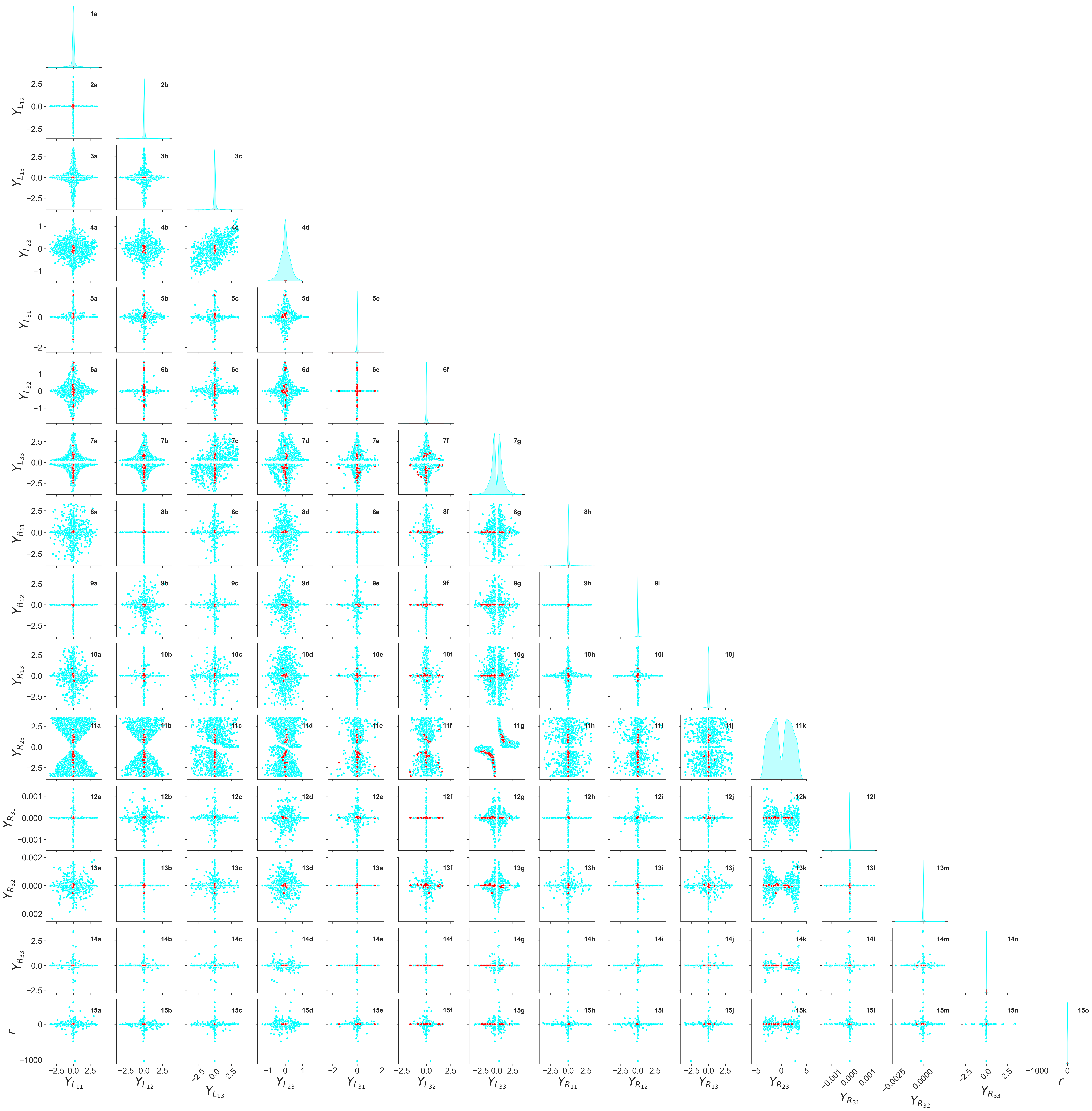
Figure 3: Pairwise correlation plot between various Yukawa matrix ${\mathcal{Y}_{1}^{L}},{\mathcal{Y}_{1}^{R}}$ elements, as well as the parameter $r$ of the $\mathbb{R}$ matrix, in the presence of $R_{D},R_{D}^{\ast}$ anomaly (Case I). The cyan points satisfy the constraints from cLFV decays, LFUV ratios, $B\,\rightarrow\,K\,\nu\,\nu$ constraints and generate the correct order of magnitude for neutrino masses and oscillation parameters. Red points survive after putting the constraint from $\mu\to e$ conversion in Au nucleus.

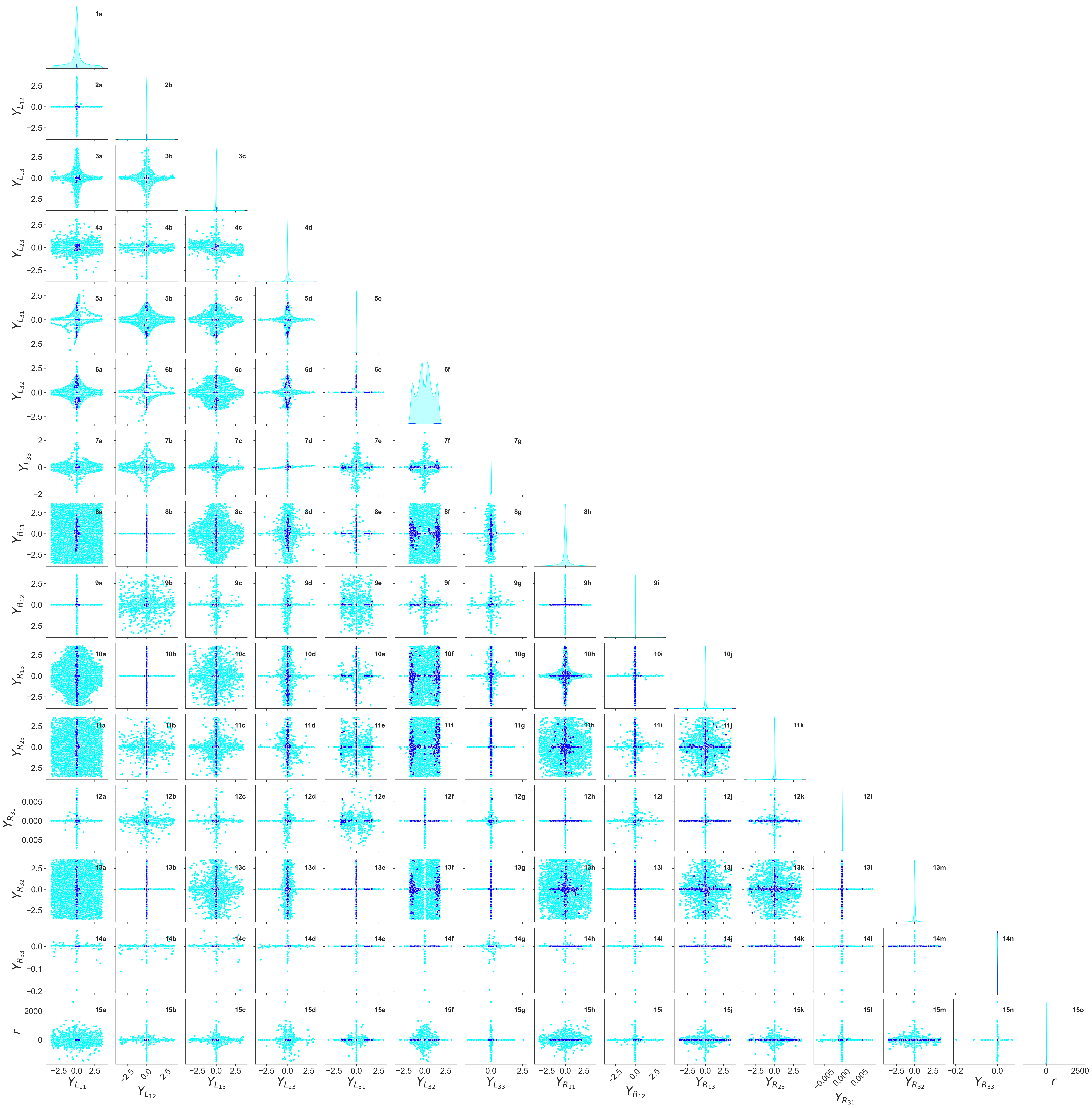
Figure 4: Pairwise correlation plot between various Yukawa matrix ${\mathcal{Y}_{1}^{L}},{\mathcal{Y}_{1}^{R}}$ elements as well as the parameter $r$ of the $\mathbb{R}$ matrix, in the hypothetical scenario where $R_{D},R_{D}^{\ast}$ anomaly is gone (Case II). The cyan points satisfy the constraints from cLFV decays, LFUV ratios in Case II, $B\,\rightarrow\,K\,\nu\,\nu$ constraints and generate the correct order of magnitude for neutrino masses and oscillation parameters. Blue points survive after putting the constraint from $\mu\to e$ conversion in Au nucleus.

VI.2 Results

Now, to capture the interplay between the different elements of Yukawa matrices, we have presented Figs. 3 and 4 where we study the pairwise correlations between different elements of the Yukawa matrices ${\mathcal{Y}_{1}^{L}}$ and ${\mathcal{Y}_{1}^{R}}$, as well as the parameter $r$ appearing in the $\mathbb{R}$ matrix [cf. Eq. (87)]. In both figures, the rightmost panel in each row has the same parameter on the $x$ and $y$ axes; hence, these are just the distributions over which a particular parameter is varied. In our analysis, we have considered two different cases for the $R_{D^{(*)}}$ observables:

1. Case I: $R_{D},R_{D^{*}}$ are anomalous, i.e the experimental values of $R_{D},R_{D^{*}}$ are not consistent with the SM predictions, which seems to be the current situation [cf. Eq. (67)]. Fig. 3 refers to this case.

2. Case II: This is a hypothetical scenario where the experimental values of $R_{D},R_{D^{*}}$ are consistent with the SM predictions within the $1\sigma$ error bars. In this case, we consider $\Delta r_{D^{(*)}}=\left|r_{D^{(*)}}-r_{D^{(*)}}^{\rm SM}\right|<10^{-3}$. Fig. 4 refers to this case.

In both Figs. 3 and 4, the cyan points produce the correct neutrino mass as well as oscillation parameters, satisfy the current constraints from cLFV decays ($\mu\rightarrow\,e\,\gamma\,\,,\,\tau\rightarrow\,\mu\,\gamma$ and $\tau\rightarrow\,e\,\gamma$), the rare $B$ and $K$ meson decays listed in Subsection V.2 and also can reproduce the observed value of electron $(g-2)$ (either Cs or Rb-based value). Note that in Fig. 3, due to a strong tension with the current $R_{D^{(\ast)}}$ results, the $1\sigma$ value of $\Delta a_{\mu}$ is hard to achieve in these regions, even with the BMW result for the SM prediction. This point will be further elaborated later. The red points are obtained after putting the constraint coming from $\mu\to e$ conversion in Gold (Au) nucleus. From here, we can infer that this process gives the most stringent constraint on the Yukawa couplings and much of the otherwise allowed parameter space gets disfavored. The strongest anti-correlation is seen in panel ($11g$) which indicates that the dominant contribution to $R_{D}$ and $R_{D^{\ast}}$ comes from $C_{S_{L}}$ [cf. Eq. (61)] which involves ${Y_{L_{33}}}$ and ${Y_{R_{23}}}$. Panel (11g) also implies that ${Y_{L_{33}}}{Y_{R_{23}}}>0$, otherwise, the leptoquark contribution will destructively interfere with the SM contribution and Eq. (67) will be smaller than one.

Fig. 4 shows the correlation between the same Yukawa matrix elements and $r$, like in Fig. 3, but with the assumption that $R_{D}-R_{D^{\ast}}$ are consistent with the SM predictions (Case II). As a result, the parameter space represented by the cyan points get enlarged as compared to Case I and certain correlations or anti-correlations among the pair of respective Yukawa couplings, observed in the earlier figure, vanish. In panel (11g), now the points near to origin (0,0) are allowed as the $R_{D}-R_{D^{\ast}}$ anomaly is absent in this case. However, the $\mu\to e$ conversion still puts the most stringent constraint in this case also and disfavors a large part of the parameter space. The final surviving points are shown in blue.

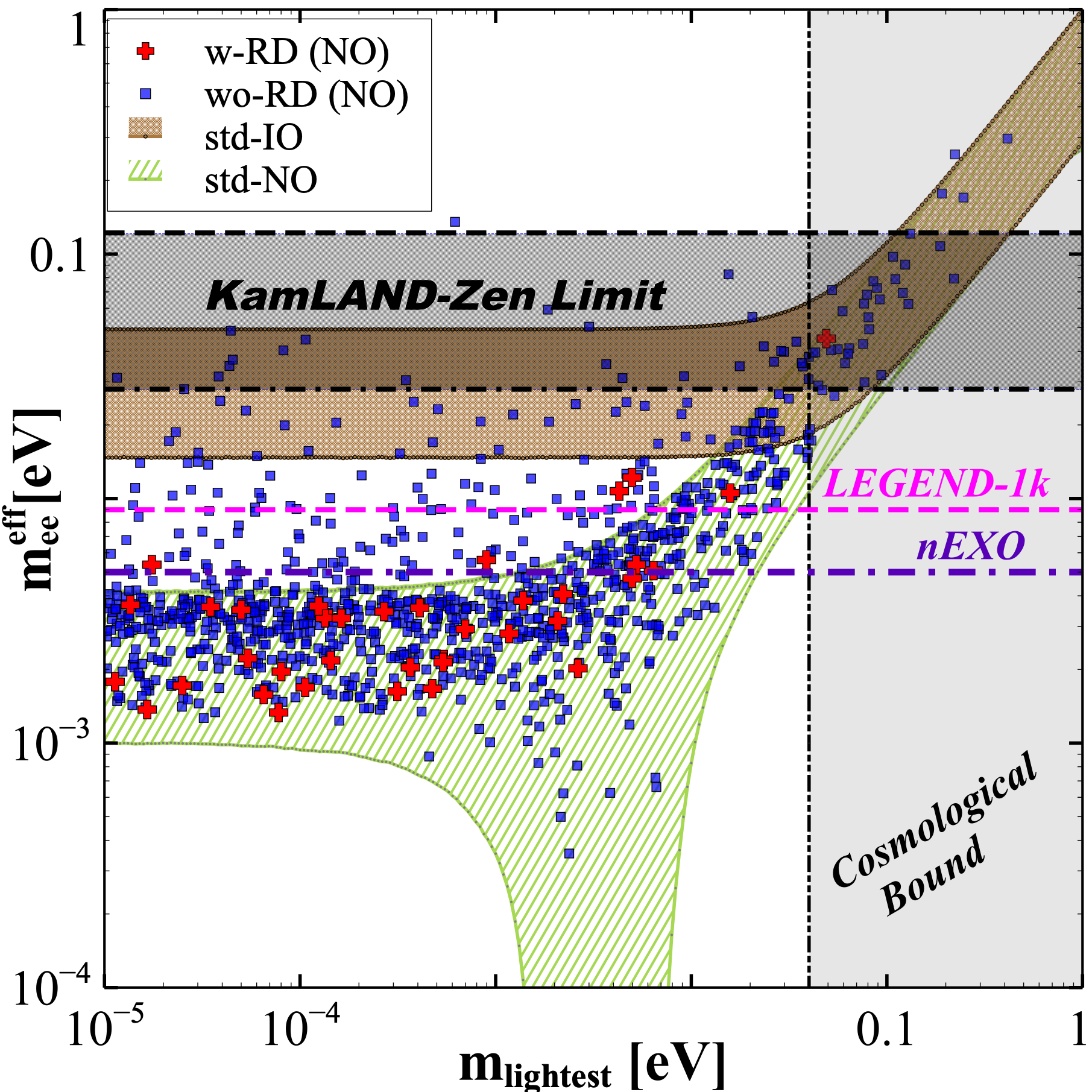
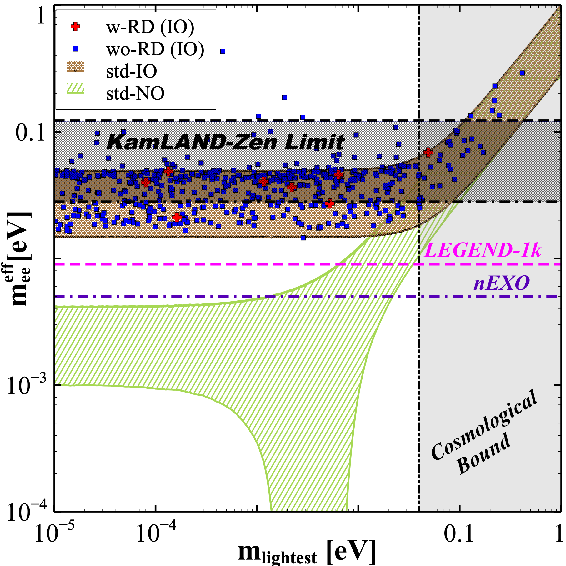
Figure 5: Plot of $m_{ee}^{\rm eff}$ as a function of the lightest neutrino mass where active neutrino masses obey NO (left panel) and IO (right panel). The standard NO and IO regions are denoted by lime green hatched and brown shaded regions, respectively. The blue squares (red plus) denote the $m_{ee}^{\rm eff}$ contributions in Case I and II, respectively. The dark grey shaded horizontal region denotes the current KamLAND-Zen upper bound on $m_{ee}$ for different NMEs while the magenta dashed (purple dot-dashed) line denotes the future reach of LEGEND-1000 (nEXO) on $m_{ee}$. The vertical light grey shaded region represents the excluded range from the cosmological limit on the sum of light neutrino masses.

Now that we have identified the allowed leptoquark parameter space from the flavor observables and neutrino mass constraints, we proceed to study the $0\nu\beta\beta$ predictions. In Fig. 5, we have plotted $m_{ee}^{\rm eff}$ [cf. Eq. (23)] as a function of the lightest neutrino mass for values of Yukawa couplings that are allowed from the combined analysis as presented in Figs. 3 and 4. The oscillation parameters are varied in their allowed $3\sigma$ range nufit , and the Majorana phases are varied in the range ($0:\pi$). In the left (right) panel the blue squares [red plus] denote the values of $m_{ee}^{\rm eff}$ after including the leptoquark contributions for NO (IO) for Case II [I]. In both panels, the standard contribution to $m_{ee}^{\rm eff}$ for NO (grey hatched) and IO (brown shaded) are displayed for comparison purpose. Also, the current bound on $m_{ee}$ from KamLAND-Zen experiment KamLAND-Zen:2024eml and the future projections from LEGEND-1000 LEGEND:2021bnm and nEXO nEXO:2021ujk are shown using dark grey shaded (with the band representing NME uncertainties), magenta dashed and purple dot-dashed lines respectively. The cosmologically disfavored region is denoted by the grey vertical band from Planck data Planck:2018vyg . From the left panel, we see that the cancellation region found in the standard 3-flavor picture is no longer there when leptoquark contributions are added. For some values of parameters, $m_{ee}^{\rm eff}$ can exceed the maximum value of the standard scenario. Most of these regions can be explored in the future ton-scale experiments like LEGEND-1000 and nEXO, as can be seen from the figure. In the scanned region, $m_{ee}^{\rm eff}$ for NO including the leptoquark contribution goes into the standard IO region. In order to distinguish the standard IO region without leptoquarks from NO region with leptoquarks, just $0\nu\beta\beta$ is not enough, and we need additional flavor and/or collider observables. This is why the study of $0\nu\beta\beta$ correlations with other observables is so important. On the other hand, for IO (right panel), adding the leptoquark contribution does not make any drastic change to the standard predictions, although there are a few points which give a higher contribution and are already disfavored by the current KamLAND-Zen upper bound on $m_{ee}$.

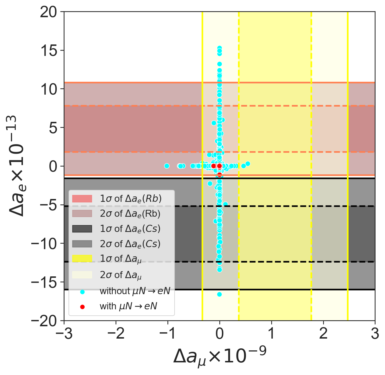
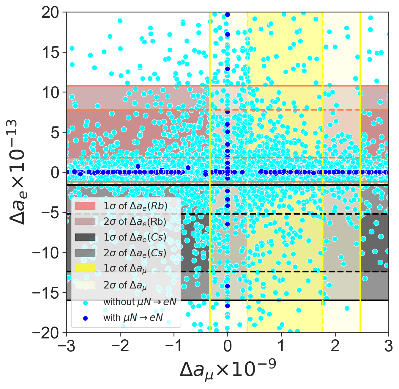
Figure 6: Left Panel: Plot of $\Delta a_{\mu}$ vs $\Delta a_{e}$ in our leptoquark scenario satisfying current experimental limits on $R_{D}$-$R_{D^{*}}$ (Case I). Right Panel: Assuming $R_{D}$-$R_{D^{*}}$ is no longer anomalous. The cyan points satisfy all constraints except $\mu\to e$ conversion, and red (blue) points also satisfy $\mu\to e$ conversion bound for Case I (Case II). The vertical yellow shaded bands show the $1\sigma$ and $2\sigma$ allowed ranges of $\Delta a_{\mu}$, whereas the horizontal coral (grey) shaded bands show the $1\sigma$ and $2\sigma$ allowed ranges of $\Delta a_{e}$ for Rb (Cs).

In Fig. 6, we demonstrate the tension between the electron and muon $(g-2)$ anomalies, and the $R_{D},R_{D^{*}}$ anomalies. The left panel is for Case I (with $R_{D^{(*)}}$ being anomalous) and the right panel is for Case II (where $R_{D^{(*)}}$ is consistent with the SM). In both figures, the cyan points satisfy the cLFV decay constraints (excluding the $\mu\to e$ conversion) and rare meson decays, whereas the red (blue) points in Case I (II) also include the $\mu\to e$ conversion bound. The dark (light) yellow shaded region correspond to the $1\sigma$ ($2\sigma$) region of $\Delta a_{\mu}$ taking the BMW result for the SM prediction. It is seen from the left panel that with $R_{D},R_{D^{*}}$ not consistent with the SM prediction, the allowed points cannot accommodate muon $(g-2)$ in its $1\sigma$ range. This occurs because, to satisfy $R_{D}-R_{D^{\ast}}$, ${Y_{L_{33}}}$ must be at least $\sim\mathcal{O}(0.1)$. This constraint forces ${Y_{L_{32}}}$ and ${Y_{R_{32}}}$ to remain small to comply with the $\tau\rightarrow\mu\,\gamma$ limit, resulting in very small values of $\Delta a_{\mu}$. If the constraints coming from $R_{D},R_{D^{*}}$ are relaxed as in the right panel, then the muon $(g-2)$ can be satisfied at $1\sigma$ as well. This is because the absence of the $R_{D}-R_{D^{\ast}}$ anomaly suggests small values of ${Y_{L_{33}}}$. Thus, even with the sizable values of ${Y_{L_{23}}}$ and ${Y_{R_{23}}}$, constraints from $\tau\rightarrow\mu\gamma$ can be avoided. If the constraints from $\mu\rightarrow e$ conversion are included then the allowed region is further constrained severely, especially in Case I. As seen from the left panel there are no points that can reach the $1\sigma$ value of $\Delta a_{\mu}$. In the right panel also, the allowed parameters are severely restricted after putting the $\mu\to e$ conversion constraint. However, $\Delta a_{\mu}$ can be satisfied even in its $1\sigma$ range.

In Fig. 6, the dark (light) coral shaded region correspond to the $1\sigma$ ($2\sigma$) range of $\Delta a_{e}$ for Rb. The black (grey) shaded region represent the same for the Cs. It is seen from both panels that the cyan points can reach the $1\sigma$ range of $\Delta a_{e}$ value. However, when $\mu\to e$ conversion constraint is applied, in Case I, $\Delta a_{e}$ is satisfied for Rb only at $2\sigma$ level, whereas it cannot be satisfied for Cs. On the other hand, for Case II, $\Delta a_{e}$ can be satisfied at $1\sigma$ level for both Rb and Cs, even after implementing the $\mu\to e$ conversion as well as all the other constraints mentioned earlier.

VI.3 Effect of Varying Leptoquark Mass

In the previous section, we have fixed the leptoquark mass at $1.5$ TeV for the parameter scanning. To see the effect of varying leptoquark mass, in this section, we fix the ${\mathcal{Y}_{1}^{L}}$ and ${\mathcal{Y}_{1}^{R}}$ matrix elements to a suitable representative benchmark value and vary the leptoquark mass to see what is its maximum allowed value that can explain the $R_{D^{(*)}}$ and $\Delta a_{\ell}$ anomalies. It is important to mention here that the following analysis is strictly valid only for the chosen benchmark values of the Yukawa couplings:

$${\mathcal{Y}_{1}^{L}} = \begin{pmatrix}0.06&0&0.0006\\ 0&0&0.04\\ 10^{-5}&-0.15&1.07\end{pmatrix},\quad\quad{\mathcal{Y}_{1}^{R}}=\begin{pmatrix}0.003&0&0\\ 0&0&0.9\\ 0&0&10^{-5}\end{pmatrix}.$$ (91)

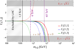
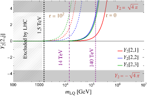
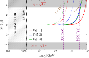
Figure 7: Variation of $Y_{2}$ elements with leptoquark mass when all the elements of ${\mathcal{Y}_{1}^{L}}$ and ${\mathcal{Y}_{1}^{R}}$ are fixed as given by Eq. (91). The solid (dashed) curves are for $r=0~{}(10^{2})$. The horizontal shaded regions represent the perturbativity limit on the Yukawa couplings. The vertical hatched region is excluded by LHC searches for leptoquarks.

Once ${\mathcal{Y}_{1}^{L}}$ and ${\mathcal{Y}_{1}^{R}}$ are fixed to the above values, the ${\mathcal{Y}_{2}}$ elements are determined from Eq. (86), giving the input parameters as discussed in the earlier Section. In Fig. 7, we have shown the variation of the elements of ${\mathcal{Y}_{2}}$ as a function of the leptoquark mass for two different values of $r$. The hatched region on the left corresponds to the collider bound on $m_{\rm LQ}>1280$ GeV from direct LHC searches ParticleDataGroup:2022pth . The vertical lines correspond to the different leptoquark masses as depicted in the figure. It is seen that the magnitude of the ${\mathcal{Y}_{2}}$ matrix elements increases with increasing leptoquark mass. This is because as $m_{\rm LQ}$ grows, $\frac{m_{X_{1}}}{m_{X_{2}}}\,\rightarrow\,1$ [cf. Eq. 7]; therefore, the value of ${\mathcal{Y}_{2}}$ must increase to generate neutrino masses of the $\mathcal{O}(10^{-2})$ eV [cf. Eq. (9)]. As ${\mathcal{Y}_{2}}$ is proportional to $\mathbb{R}$ [cf. Eq. (86)], it also increases with $r$ for a given value of the leptoquark mass. From this figure, we find that the elements of ${\mathcal{Y}_{2}}$ matrix exceed the perturbativity limit for $m_{\rm LQ}\,>65~{}(6)$ TeV for $r=0~{}(100)$. So, large values of $r$ are not allowed by the perturbativity conditions of the elements of ${\mathcal{Y}_{2}}$ matrix.

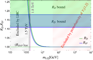
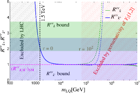
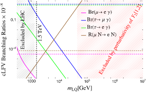
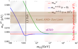
Figure 8: Upper left: Variation of $R_{D}$ (green) and $R_{D^{\ast}}$ (blue) as a function of leptoquark mass. The green (light blue) shaded region corresponds to the current experimental values on $R_{D}$ ($R_{D^{\ast}}$). The green dashed line corresponds to the SM prediction. Upper right: $R_{K}^{\nu\nu}$ (green) and $R_{K^{\ast}}^{\nu\nu}$ (blue) as a function of leptoquark mass for three values of $r$. The green-shaded region corresponds to the current experimental value on $R_{K}^{\nu\nu}$, and the light blue-shaded region shows the experimental limit on ($R_{K^{\ast}}^{\nu\nu}$). Lower left: BRs of cLFV decays as a function of the leptoquark mass. Magenta, blue, green and brown curves correspond to BRs of $\mu\rightarrow\,e\,\gamma$, $\tau\rightarrow\,\mu\,\gamma$, $\tau\rightarrow\,e\,\gamma$ and $\mu\to e$ conversion ratio respectively, and the horizontal lines denote their experimental limits. Lower right: Variation of $m_{ee}^{\rm eff}$ as a function of $m_{\rm LQ}$ for different values of $r$. The solid red line denotes the standard contribution for NO. The horizontal shaded band is the current KamLAND-Zen limit, and the brown dashed line is the future nEXO projection.

Fig. 8 shows the variation of $R_{D}$, $R_{D^{\ast}}$, $R_{K}^{\nu\nu}$, $R_{K^{\ast}}^{\nu\nu}$, cLFV decay BRs , $\mu\to e$ conversion rate and the $m_{ee}^{eff}$ as a function of the leptoquark mass. From the left most panel, it is inferred that only a small region of $m_{\rm LQ}$ around 1.5 TeV scale is allowed for the current values of $R_{D}$ and $R_{D^{\ast}}$. As $m_{\rm LQ}$ increases, the value $R_{D}$-$R_{D^{\ast}}$ decreases and gradually converge to the SM value, and hence, the anomaly can not be explained. In the case of $R_{K}^{\nu\nu}$ and $R_{K^{\ast}}^{\nu\nu}$, an upturn is seen above a certain value of leptoquark mass. As can be seen in Eq. (75), $R_{K}^{\nu\nu}$ and $R_{K^{\ast}}^{\nu\nu}$ depend on $C_{L}$ and $C_{R}$, which are proportional to ${\mathcal{Y}_{1}^{L}}$ and ${\mathcal{Y}_{2}}$, respectively. Below a certain value of $m_{\rm LQ}$, ${\mathcal{Y}_{2}}$ is very small, and $C_{L}$ dominates in this region. However, as $m_{\rm LQ}$ increases, ${\mathcal{Y}_{2}}$ also increases, causing $C_{R}$ to dominate, and therefore, increases $R_{K}^{\nu\nu}$ and $R_{K^{\ast}}^{\nu\nu}$. Since ${\mathcal{Y}_{2}}$ also increases with $r$, for larger $r$ values, the upturn is seen at smaller $m_{\rm LQ}$ values. The BRs of cLFV decay are inversely proportional to the leptoquark mass and gradually decrease as $m_{\rm LQ}$ increases as can be seen in the lower left panel of Fig. (8).

However, the $\mu\to e$ conversion rate shows a different trend as it is seen to rise with the value of the leptoquark mass. This can be understood from Eq. (27) where we see that the parameter $C_{V_{LR}}^{d}$ contributing to the rate increases with ${\mathcal{Y}_{2}}$ and decreases with $m_{\rm LQ}$ . From Fig. 7 it is also seen that as the value of $m_{\rm LQ}$ becomes higher, ${\mathcal{Y}_{2}}$ increases. Overall, the interplay of these two parameters causes $C_{V_{LR}}^{d}$ to increase, thus enhancing the conversion rate. As a result, a stringent bound on the leptoquark mass ($\leq$ 3.5 TeV) emerges from the current observed limits on the $\mu\to e$ conversion rate for the chosen benchmark values of Yukawa couplings.

From the lower right panel of Fig. 8, it is observed that $m_{ee}^{\rm eff}$ for NO decreases as $m_{\rm LQ}$ increases, and for higher values of leptoquark mass, approaches the standard contribution (red solid line). However, there are certain leptoquark masses, where due to destructive interference the leptoquark contribution can be lower than the standard contribution. The leptoquark contribution can be higher than the standard contribution for higher values of $m_{\rm LQ}$ if $r$ is larger, since the latter enhances the $\left({\mathcal{Y}_{2}}\right)_{11}$ element. Therefore, depending on $r$, the leptoquark contribution can set an upper bound on $m_{\rm LQ}$ from the KamLAND-Zen current limit or future $0\nu\beta\beta$ experiments.

VII Conclusions

Scalar leptoquarks provide an attractive framework for neutrino mass generation radiatively. At the same time, the new leptoquark interactions give rise to new contributions to various lepton number and flavor violating processes. We have considered the Standard Model augmented with two scalar leptoquarks. While a single leptoquark cannot generate correct neutrino mass, the combination of singlet-doublet leptoquarks ($S_{1}-\tilde{R}_{2}$) can generate the neutrino mass radiatively. Such models have a rich phenomenology since leptoquarks can couple to both quarks and leptons. Our main aim was to study the implications of this combination in context of neutrinoless double beta decay. To find the allowed values of the Yukawa couplings, we imposed the constraints from neutrino mass and mixing, as well as demanded compliance with bounds coming from charged lepton flavor violation, lepton flavor universality violation and low-energy rare meson decays. We performed a comprehensive global parameter scan satisfying all available experimental data arising from the above-mentioned constraints, as well as existing anomalies in $R_{D^{(*)}}$ and $\Delta a_{\ell}$ to constrain the allowed parameter space for various Yukawa matrix elements with a TeV-scale leptoquark mass. Our combined analysis reveals some interesting interplay and tensions coming from different constraints. For instance, if we take the $R_{D}-R_{D^{\ast}}$ data at face value which is not consistent with the SM prediction, there is a strong tension with the muon $(g-2)$, which cannot be explained within its $1\sigma$ range. On the other hand, if in the near future, the $R_{D}-R_{D^{\ast}}$ value becomes consistent with the SM value then the allowed parameters can be made consistent with the muon $(g-2)$. We found that that the most stringent constraints on the allowed Yukawa couplings are obtained from $\mu\rightarrow e$ conversion in nuclei. We obtained the prediction for $m_{ee}^{\rm eff}$, arising from the combined contributions of standard and leptoquark contributions, for the Yukawa coupling values that pass all the above mentioned constraints. We find that the contribution from leptoquark mediated diagrams to $m_{ee}^{\rm eff}$ can be significant and even greater than the standard contribution for normal ordering of the light neutrinos and the cancellation region is no longer present around $m_{\rm{lightest}}\sim{\rm meV}$. The total value of $m_{ee}^{\rm eff}$ can lie in the desert region between the standard NO and IO regions and hence can be probed by future experiments like LEGEND-1000 and nEXO.

We have also varied the leptoquark mass fixing some benchmark values of Yukawa couplings and discussed the constraints on this from different observables, as well as from the perturbativity bounds. For the chosen parameter values, we find very stringent constraint on leptoquark mass, $m_{\rm LQ}<3.5$ TeV, from the $\mu\to e$ conversion rate. Compliance with observed $R_{D}-R_{D^{\ast}}$ imposes an even stronger bound, $m_{\rm LQ}<1.8$ TeV, which is on the verge of being ruled out by direct searches in the Run 3 phase of the LHC.

Appendix A Fierz Transformation List

Calculations of low-energy weak interactions with fermions often involve superposition of quartic products of Dirac spinors, where the order of the spinors varies among the terms. A common technique to standardize their ordering is known as the Fierz transformation. The usual Fierz relation can be written as Nieves:2003in

$$e_{\Gamma}(1234) = \sum_{\Gamma^{\prime}}F_{\Gamma\,\Gamma^{\prime}}e_{\Gamma^{\prime}}(1432).$$ (92)

Here $\Gamma,\Gamma^{\prime}\in\,\{S,V,T,A,P\}$ , $F_{\Gamma\,\Gamma^{\prime}}$ are numerical coefficients and $e_{\Gamma}(1234)\equiv\left(\overline{w}_{1}\Gamma w_{2}\right)\left(\overline{w}_{3}\Gamma w_{4}\right)$, where $w_{i}$ are the spinors. In case of leptoquark interactions, we use the following Fierz relation

$$e_{S}(1234)=\frac{1}{4}\left[e_{S}(1432)+e_{V}(1432)+\frac{1}{2}e_{T}(1432)-e_{A}(1432)+e_{P}(1432)\right].$$ (93)

Then the Fierz transformation list is as follows:

$$\left(\overline{d}^{c}P_{L}\nu\right)\left(\overline{e}P_{R}u^{c}\right) =-\frac{1}{2}\left(\overline{u}\gamma^{\mu}P_{L}d\right)\left(\overline{e}\gamma_{\mu}P_{L}\nu_{L}\right),$$ (94)

$$\left(\overline{d}^{c}P_{L}\nu\right)\left(\overline{e}P_{L}u^{c}\right) =\frac{1}{2}\left(\overline{d}^{c}P_{L}u^{c}\right)\,\left(\overline{e}P_{L}\nu\right)+\frac{1}{8}\left(\overline{d}^{c}\sigma^{\mu\nu}P_{L}u^{c}\right)\,\left(\overline{e}\sigma_{\mu\nu}P_{L}\nu\right)$$

$$=\frac{1}{2}\left(\overline{u}P_{L}d\right)\,\left(\overline{e}P_{L}\nu\right)-\frac{1}{8}\left(\overline{u}\sigma^{\mu\nu}P_{L}d\right)\,\left(\overline{e}\sigma_{\mu\nu}P_{L}\nu\right),$$ (95)

$$\left(\overline{d}^{c}P_{R}\nu^{c}\right)\left(\overline{e}P_{R}u^{c}\right) =\frac{1}{2}\left(\overline{d}^{c}P_{R}u^{c}\right)\left(\overline{e}P_{R}\nu^{c}\right)+\frac{1}{8}\left(\overline{d}^{c}\sigma^{\mu\nu}P_{R}u^{c}\right)\left(\overline{e}\sigma_{\mu\nu}P_{R}\nu^{c}\right)$$

$$=\frac{1}{2}\left(\overline{u}P_{R}d\right)\left(\overline{e}P_{R}\nu^{c}\right)-\frac{1}{8}\left(\overline{u}\sigma^{\mu\nu}P_{R}d\right)\left(\overline{e}\sigma_{\mu\nu}P_{R}\nu^{c}\right),$$ (96)

$$\left(\overline{d}^{c}P_{R}\nu^{c}\right)\left(\overline{e}P_{L}u^{c}\right) =\frac{1}{2}\left(\overline{d}^{c}\gamma^{\mu}P_{L}u^{c}\right)\left(\overline{e}\gamma_{\mu}P_{R}\nu^{c}\right)\,=\,-\frac{1}{2}\left(\overline{u}\gamma^{\mu}P_{R}d\right)\left(\overline{e}\gamma_{\mu}P_{R}\nu^{c}\right).$$ (97)

Appendix B Loop Functions for cLFV

The loop functions $\mathcal{F}(x)$ and $\mathcal{G}(x)$ appearing in Eqs. (34)-(37) can be defined as

$$\mathcal{F}(x) = Q_{S}f_{S}(x)-f_{F}(x)\,,\qquad\mathcal{G}(x)=Q_{S}\,g_{S}(x)-g_{F}(x),$$ (98)

where $Q_{S}$ is the electromagnetic charge for the scalar leptoquark and

$$f_{S}(x) = \frac{x+1}{4(1-x)^{2}}+\frac{x\,\ln x}{2(1-x)^{3}},$$ (99)

$$f_{F}(x) = \frac{x^{2}-5x-2}{12(x-1)^{3}}+\frac{x\,\ln x}{2(x-1)^{4}},$$ (100)

$$g_{S}(x) = \frac{1}{x-1}-\frac{\ln x}{(x-1)^{2}},$$ (101)

$$g_{F}(x) = \frac{x-3}{2(x-1)^{2}}+\frac{\ln x}{(x-1)^{3}}.$$ (102)

For $x\ll 1$, these loop functions can be approximated as

$$f_{S}(x) \simeq \frac{1}{4},\quad f_{F}(x)\simeq\frac{1}{6},\quad g_{S}(x)\simeq-\ln(x),\quad g_{F}(x)\simeq-\ln(x)\,.$$ (103)

Note that for leptoquark $\widetilde{R}_{2}^{2/3}$ with $Q_{S}=2/3$, we have $\mathcal{F}(x)\sim\frac{2}{3}\times\frac{1}{4}-\frac{1}{6}=0$.

References

- (1) Super-Kamiokande Collaboration, Y. Fukuda et al., “Evidence for oscillation of atmospheric neutrinos,” Phys. Rev. Lett. 81 (1998) 1562–1567, [hep-ex/9807003].
- (2) SNO Collaboration, Q. R. Ahmad et al., “Direct evidence for neutrino flavor transformation from neutral current interactions in the Sudbury Neutrino Observatory,” Phys. Rev. Lett. 89 (2002) 011301, [nucl-ex/0204008].
- (3) S. Weinberg, “Baryon and Lepton Nonconserving Processes,” Phys. Rev. Lett. 43 (1979) 1566–1570.
- (4) NuFIT Collaboration, “Three-neutrino fit based on data available in march 2024.” www.nu-fit.org.
- (5) Particle Data Group Collaboration, R. L. Workman et al., “Review of Particle Physics,” PTEP 2022 (2022) 083C01.
- (6) Planck Collaboration, N. Aghanim et al., “Planck 2018 results. VI. Cosmological parameters,” Astron. Astrophys. 641 (2020) A6, [1807.06209]. [Erratum: Astron.Astrophys. 652, C4 (2021)].
- (7) P. Minkowski, “ at a Rate of One Out of Muon Decays?,” Phys. Lett. B 67 (1977) 421–428.
- (8) R. N. Mohapatra and G. Senjanovic, “Neutrino Mass and Spontaneous Parity Nonconservation,” Phys. Rev. Lett. 44 (1980) 912.
- (9) T. Yanagida, “Horizontal gauge symmetry and masses of neutrinos,” Conf. Proc. C 7902131 (1979) 95–99.
- (10) M. Gell-Mann, P. Ramond, and R. Slansky, “Complex Spinors and Unified Theories,” Conf. Proc. C 790927 (1979) 315–321, [1306.4669].
- (11) R. N. Mohapatra, “Mechanism for Understanding Small Neutrino Mass in Superstring Theories,” Phys. Rev. Lett. 56 (1986) 561–563.
- (12) R. N. Mohapatra and J. W. F. Valle, “Neutrino Mass and Baryon Number Nonconservation in Superstring Models,” Phys. Rev. D 34 (1986) 1642.
- (13) E. K. Akhmedov, M. Lindner, E. Schnapka, and J. W. F. Valle, “Left-right symmetry breaking in NJL approach,” Phys. Lett. B 368 (1996) 270–280, [hep-ph/9507275].
- (14) M. Malinsky, J. C. Romao, and J. W. F. Valle, “Novel supersymmetric SO(10) seesaw mechanism,” Phys. Rev. Lett. 95 (2005) 161801, [hep-ph/0506296].
- (15) M. B. Gavela, T. Hambye, D. Hernandez, and P. Hernandez, “Minimal Flavour Seesaw Models,” JHEP 09 (2009) 038, [0906.1461].
- (16) J. Barry, W. Rodejohann, and H. Zhang, “Light Sterile Neutrinos: Models and Phenomenology,” JHEP 07 (2011) 091, [1105.3911].
- (17) S. K. Kang and C. S. Kim, “Extended double seesaw model for neutrino mass spectrum and low scale leptogenesis,” Phys. Lett. B 646 (2007) 248–252, [hep-ph/0607072].
- (18) P. S. B. Dev and A. Pilaftsis, “Minimal Radiative Neutrino Mass Mechanism for Inverse Seesaw Models,” Phys. Rev. D 86 (2012) 113001, [1209.4051].
- (19) A. Zee, “A Theory of Lepton Number Violation, Neutrino Majorana Mass, and Oscillation,” Phys. Lett. B 93 (1980) 389. [Erratum: Phys.Lett.B 95, 461 (1980)].
- (20) K. S. Babu, “Model of ’Calculable’ Majorana Neutrino Masses,” Phys. Lett. B 203 (1988) 132–136.
- (21) Y. Cai, J. Herrero-García, M. A. Schmidt, A. Vicente, and R. R. Volkas, “From the trees to the forest: a review of radiative neutrino mass models,” Front. in Phys. 5 (2017) 63, [1706.08524].
- (22) K. S. Babu, P. S. B. Dev, S. Jana, and A. Thapa, “Non-Standard Interactions in Radiative Neutrino Mass Models,” JHEP 03 (2020) 006, [1907.09498].
- (23) S. Dimopoulos and L. Susskind, “Mass Without Scalars,” Nucl. Phys. B 155 (1979) 237–252.
- (24) J. C. Pati and A. Salam, “Unified Lepton-Hadron Symmetry and a Gauge Theory of the Basic Interactions,” Phys. Rev. D 8 (1973) 1240–1251.
- (25) H. Fritzsch and P. Minkowski, “Unified Interactions of Leptons and Hadrons,” Annals Phys. 93 (1975) 193–266.
- (26) I. Doršner, S. Fajfer, A. Greljo, J. F. Kamenik, and N. Košnik, “Physics of leptoquarks in precision experiments and at particle colliders,” Phys. Rept. 641 (2016) 1–68, [1603.04993].
- (27) D. Zhang, “Radiative neutrino masses, lepton flavor mixing and muon g 2 in a leptoquark model,” JHEP 07 (2021) 069, [2105.08670].
- (28) S. Parashar, A. Karan, Avnish, P. Bandyopadhyay, and K. Ghosh, “Phenomenology of scalar leptoquarks at the LHC in explaining the radiative neutrino masses, muon g-2, and lepton flavor violating observables,” Phys. Rev. D 106 no. 9, (2022) 095040, [2209.05890].
- (29) D. Aristizabal Sierra, M. Hirsch, and S. G. Kovalenko, “Leptoquarks: Neutrino masses and accelerator phenomenology,” Phys. Rev. D 77 (2008) 055011, [0710.5699].
- (30) Y. Cai, J. D. Clarke, M. A. Schmidt, and R. R. Volkas, “Testing Radiative Neutrino Mass Models at the LHC,” JHEP 02 (2015) 161, [1410.0689].
- (31) I. Doršner, S. Fajfer, and N. Košnik, “Leptoquark mechanism of neutrino masses within the grand unification framework,” Eur. Phys. J. C 77 no. 6, (2017) 417, [1701.08322].
- (32) L. J. Hall and M. Suzuki, “Explicit R-Parity Breaking in Supersymmetric Models,” Nucl. Phys. B 231 (1984) 419–444.
- (33) M. Hirsch, H. V. Klapdor-Kleingrothaus, and S. G. Kovalenko, “New leptoquark mechanism of neutrinoless double beta decay,” Phys. Rev. D 54 (1996) R4207–R4210, [hep-ph/9603213].
- (34) L. Lavoura, “General formulae for f(1) — f(2) gamma,” Eur. Phys. J. C 29 (2003) 191–195, [hep-ph/0302221].
- (35) R. Benbrik and C.-K. Chua, “Lepton Flavor Violating and Decays Induced by Scalar Leptoquarks,” Phys. Rev. D 78 (2008) 075025, [0807.4240].
- (36) S. Fajfer, N. Košnik, and L. Vale Silva, “Footprints of leptoquarks: from to ,” Eur. Phys. J. C 78 no. 4, (2018) 275, [1802.00786].
- (37) S. Descotes-Genon, S. Fajfer, J. F. Kamenik, and M. Novoa-Brunet, “Implications of anomalies for future measurements of and ,” Phys. Lett. B 809 (2020) 135769, [2005.03734]. [Addendum: Phys.Lett.B 840, 137830 (2023)].
- (38) F. F. Deppisch, K. Fridell, and J. Harz, “Constraining lepton number violating interactions in rare kaon decays,” JHEP 12 (2020) 186, [2009.04494].
- (39) BaBar Collaboration, J. P. Lees et al., “Measurement of an Excess of Decays and Implications for Charged Higgs Bosons,” Phys. Rev. D 88 no. 7, (2013) 072012, [1303.0571].
- (40) LHCb Collaboration, R. Aaij et al., “Measurement of the ratios of branching fractions and ,” Phys. Rev. Lett. 131 (2023) 111802, [2302.02886].
- (41) Belle Collaboration, G. Caria et al., “Measurement of and with a semileptonic tagging method,” Phys. Rev. Lett. 124 no. 16, (2020) 161803, [1910.05864].
- (42) Belle-II Collaboration, I. Adachi et al., “A test of lepton flavor universality with a measurement of using hadronic tagging at the Belle II experiment,” [2401.02840].
- (43) Muon g-2 Collaboration, G. W. Bennett et al., “Final Report of the Muon E821 Anomalous Magnetic Moment Measurement at BNL,” Phys. Rev. D 73 (2006) 072003, [hep-ex/0602035].
- (44) Muon g-2 Collaboration, D. P. Aguillard et al., “Measurement of the Positive Muon Anomalous Magnetic Moment to 0.20 ppm,” Phys. Rev. Lett. 131 no. 16, (2023) 161802, [2308.06230].
- (45) Y. Sakaki, M. Tanaka, A. Tayduganov, and R. Watanabe, “Testing leptoquark models in ,” Phys. Rev. D 88 no. 9, (2013) 094012, [1309.0301].
- (46) M. Bauer and M. Neubert, “Minimal Leptoquark Explanation for the , , and Anomalies,” Phys. Rev. Lett. 116 no. 14, (2016) 141802, [1511.01900].
- (47) O. Popov and G. A. White, “One Leptoquark to unify them? Neutrino masses and unification in the light of , and anomalies,” Nucl. Phys. B 923 (2017) 324–338, [1611.04566].
- (48) Y. Cai, J. Gargalionis, M. A. Schmidt, and R. R. Volkas, “Reconsidering the One Leptoquark solution: flavor anomalies and neutrino mass,” JHEP 10 (2017) 047, [1704.05849].
- (49) W. Altmannshofer, P. S. B. Dev, and A. Soni, “ anomaly: A possible hint for natural supersymmetry with -parity violation,” Phys. Rev. D 96 no. 9, (2017) 095010, [1704.06659].
- (50) A. Angelescu, D. Bečirević, D. A. Faroughy, F. Jaffredo, and O. Sumensari, “Single leptoquark solutions to the B-physics anomalies,” Phys. Rev. D 104 no. 5, (2021) 055017, [2103.12504].
- (51) B. Capdevila, A. Crivellin, and J. Matias, “Review of Semileptonic Anomalies,” Eur. Phys. J. ST 1 (2023) 20, [2309.01311].
- (52) A. Angelescu, D. Bečirević, D. A. Faroughy, and O. Sumensari, “Closing the window on single leptoquark solutions to the -physics anomalies,” JHEP 10 (2018) 183, [1808.08179].
- (53) J. Schechter and J. W. F. Valle, “Neutrinoless Double beta Decay in SU(2) x U(1) Theories,” Phys. Rev. D 25 (1982) 2951.
- (54) EXO-200 Collaboration, G. Anton et al., “Search for Neutrinoless Double- Decay with the Complete EXO-200 Dataset,” Phys. Rev. Lett. 123 no. 16, (2019) 161802, [1906.02723].
- (55) GERDA Collaboration, M. Agostini et al., “Final Results of GERDA on the Search for Neutrinoless Double- Decay,” Phys. Rev. Lett. 125 no. 25, (2020) 252502, [2009.06079].
- (56) CUORE Collaboration, D. Q. Adams et al., “New Direct Limit on Neutrinoless Double Beta Decay Half-Life of Te128 with CUORE,” Phys. Rev. Lett. 129 no. 22, (2022) 222501, [2205.03132].
- (57) CUPID Collaboration, O. Azzolini et al., “Final Result on the Neutrinoless Double Beta Decay of 82Se with CUPID-0,” Phys. Rev. Lett. 129 no. 11, (2022) 111801, [2206.05130].
- (58) Majorana Collaboration, I. J. Arnquist et al., “Final Result of the Majorana Demonstrator’s Search for Neutrinoless Double- Decay in 76Ge,” Phys. Rev. Lett. 130 no. 6, (2023) 062501, [2207.07638].
- (59) KamLAND-Zen Collaboration, S. Abe et al., “Search for Majorana Neutrinos with the Complete KamLAND-Zen Dataset,” [2406.11438].
- (60) nEXO Collaboration, G. Adhikari et al., “nEXO: neutrinoless double beta decay search beyond 1028 year half-life sensitivity,” J. Phys. G 49 no. 1, (2022) 015104, [2106.16243].
- (61) LEGEND Collaboration, N. Abgrall et al., “The Large Enriched Germanium Experiment for Neutrinoless Decay: LEGEND-1000 Preconceptual Design Report,” [2107.11462].
- (62) M. Agostini, G. Benato, J. A. Detwiler, J. Menéndez, and F. Vissani, “Toward the discovery of matter creation with neutrinoless decay,” Rev. Mod. Phys. 95 no. 2, (2023) 025002, [2202.01787].
- (63) J. C. Helo, M. Hirsch, H. Päs, and S. G. Kovalenko, “Short-range mechanisms of neutrinoless double beta decay at the LHC,” Phys. Rev. D 88 (2013) 073011, [1307.4849].
- (64) H. Päs and E. Schumacher, “Common origin of and neutrino masses,” Phys. Rev. D 92 no. 11, (2015) 114025, [1510.08757].
- (65) M. L. Graesser, G. Li, M. J. Ramsey-Musolf, T. Shen, and S. Urrutia-Quiroga, “Uncovering a chirally suppressed mechanism of 0 decay with LHC searches,” JHEP 10 (2022) 034, [2202.01237].
- (66) L. Gráf, M. Lindner, and O. Scholer, “Unraveling the 0 decay mechanisms,” Phys. Rev. D 106 no. 3, (2022) 035022, [2204.10845].
- (67) O. Scholer, J. de Vries, and L. Gráf, “DoBe — A Python tool for neutrinoless double beta decay,” JHEP 08 (2023) 043, [2304.05415].
- (68) LHCb Collaboration, R. Aaij et al., “Test of lepton universality in decays,” Phys. Rev. Lett. 131 no. 5, (2023) 051803, [2212.09152].
- (69) LHCb Collaboration, R. Aaij et al., “Measurement of lepton universality parameters in and decays,” Phys. Rev. D 108 no. 3, (2023) 032002, [2212.09153].
- (70) Belle-II Collaboration, I. Adachi et al., “Evidence for Decays,” [2311.14647].
- (71) R. H. Parker, C. Yu, W. Zhong, B. Estey, and H. Müller, “Measurement of the fine-structure constant as a test of the Standard Model,” Science 360 (2018) 191, [1812.04130].
- (72) L. Morel, Z. Yao, P. Cladé, and S. Guellati-Khélifa, “Determination of the fine-structure constant with an accuracy of 81 parts per trillion,” Nature 588 no. 7836, (2020) 61–65.
- (73) W. Altmannshofer, P. S. B. Dev, A. Soni, and Y. Sui, “Addressing R, R, muon and ANITA anomalies in a minimal -parity violating supersymmetric framework,” Phys. Rev. D 102 no. 1, (2020) 015031, [2002.12910].
- (74) P. S. B. Dev, A. Soni, and F. Xu, “Hints of natural supersymmetry in flavor anomalies?,” Phys. Rev. D 106 no. 1, (2022) 015014, [2106.15647].
- (75) C.-K. Chua, X.-G. He, and W.-Y. P. Hwang, “Neutrino mass induced radiatively by supersymmetric leptoquarks,” Phys. Lett. B 479 (2000) 224–229, [hep-ph/9905340].
- (76) U. Mahanta, “Neutrino masses and mixing angles from leptoquark interactions,” Phys. Rev. D 62 (2000) 073009, [hep-ph/9909518].
- (77) I. Dorsner, S. Fajfer, and N. Kosnik, “Heavy and light scalar leptoquarks in proton decay,” Phys. Rev. D 86 (2012) 015013, [1204.0674].
- (78) CMS Collaboration, A. M. Sirunyan et al., “Search for pair production of second-generation leptoquarks at 13 TeV,” Phys. Rev. D 99 no. 3, (2019) 032014, [1808.05082].
- (79) CMS Collaboration, A. M. Sirunyan et al., “Search for heavy neutrinos and third-generation leptoquarks in hadronic states of two leptons and two jets in proton-proton collisions at 13 TeV,” JHEP 03 (2019) 170, [1811.00806].
- (80) CMS Collaboration, A. M. Sirunyan et al., “Search for pair production of first-generation scalar leptoquarks at 13 TeV,” Phys. Rev. D 99 no. 5, (2019) 052002, [1811.01197].
- (81) ATLAS Collaboration, M. Aaboud et al., “Searches for scalar leptoquarks and differential cross-section measurements in dilepton-dijet events in proton-proton collisions at a centre-of-mass energy of = 13 TeV with the ATLAS experiment,” Eur. Phys. J. C 79 no. 9, (2019) 733, [1902.00377].
- (82) ATLAS Collaboration, G. Aad et al., “Search for pairs of scalar leptoquarks decaying into quarks and electrons or muons in = 13 TeV collisions with the ATLAS detector,” JHEP 10 (2020) 112, [2006.05872].
- (83) CMS Collaboration, A. M. Sirunyan et al., “Search for singly and pair-produced leptoquarks coupling to third-generation fermions in proton-proton collisions at s=13 TeV,” Phys. Lett. B 819 (2021) 136446, [2012.04178].
- (84) ATLAS Collaboration, G. Aad et al., “Search for pair production of third-generation scalar leptoquarks decaying into a top quark and a -lepton in collisions at = 13 TeV with the ATLAS detector,” JHEP 06 (2021) 179, [2101.11582].
- (85) CMS Collaboration, A. Tumasyan et al., “Inclusive nonresonant multilepton probes of new phenomena at =13 TeV,” Phys. Rev. D 105 no. 11, (2022) 112007, [2202.08676].
- (86) ATLAS Collaboration, G. Aad et al., “Search for leptoquarks decaying into the b final state in collisions at = 13 TeV with the ATLAS detector,” JHEP 10 (2023) 001, [2305.15962].
- (87) ATLAS Collaboration, G. Aad et al., “Search for leptoquark pair production decaying into or in multi-lepton final states in collisions at 13 TeV with the ATLAS detector,” [2306.17642].
- (88) J. Kotila, J. Ferretti, and F. Iachello, “Long-range neutrinoless double beta decay mechanisms,” [2110.09141].
- (89) J. Barea, J. Kotila, and F. Iachello, “ and nuclear matrix elements in the interacting boson model with isospin restoration,” Phys. Rev. C 91 no. 3, (2015) 034304, [1506.08530].
- (90) J. Kotila and F. Iachello, “Phase space factors for double- decay,” Phys. Rev. C 85 (2012) 034316, [1209.5722].
- (91) B. W. Lee, C. Quigg, and H. B. Thacker, “Weak Interactions at Very High-Energies: The Role of the Higgs Boson Mass,” Phys. Rev. D 16 (1977) 1519.
- (92) M. E. Peskin and T. Takeuchi, “Estimation of oblique electroweak corrections,” Phys. Rev. D 46 (1992) 381–409.
- (93) R. Kitano, M. Koike, and Y. Okada, “Detailed calculation of lepton flavor violating muon electron conversion rate for various nuclei,” Phys. Rev. D 66 (2002) 096002, [hep-ph/0203110]. [Erratum: Phys.Rev.D 76, 059902 (2007)].
- (94) I. Plakias and O. Sumensari, “Lepton Flavor Violation in Semileptonic Observables,” [2312.14070].
- (95) S. Davidson, Y. Kuno, and A. Saporta, ““Spin-dependent” conversion on light nuclei,” Eur. Phys. J. C 78 no. 2, (2018) 109, [1710.06787].
- (96) SINDRUM II Collaboration, W. H. Bertl et al., “A Search for muon to electron conversion in muonic gold,” Eur. Phys. J. C 47 (2006) 337–346.
- (97) Mu2e Collaboration, L. Bartoszek et al., “Mu2e Technical Design Report,” [1501.05241].
- (98) COMET Collaboration, R. Abramishvili et al., “COMET Phase-I Technical Design Report,” PTEP 2020 no. 3, (2020) 033C01, [1812.09018].
- (99) T. Suzuki, D. F. Measday, and J. P. Roalsvig, “Total Nuclear Capture Rates for Negative Muons,” Phys. Rev. C 35 (1987) 2212.
- (100) I. Doršner, S. Fajfer, and O. Sumensari, “Muon and scalar leptoquark mixing,” JHEP 06 (2020) 089, [1910.03877].
- (101) MEG II Collaboration, K. Afanaciev et al., “A search for with the first dataset of the MEG II experiment,” Eur. Phys. J. C 84 no. 3, (2024) 216, [2310.12614].
- (102) Belle Collaboration, A. Abdesselam et al., “Search for lepton-flavor-violating tau-lepton decays to at Belle,” JHEP 10 (2021) 19, [2103.12994].
- (103) BaBar Collaboration, B. Aubert et al., “Searches for Lepton Flavor Violation in the Decays tau+- — e+- gamma and tau+- — mu+- gamma,” Phys. Rev. Lett. 104 (2010) 021802, [0908.2381].
- (104) Belle-II Collaboration, L. Aggarwal et al., “Snowmass White Paper: Belle II physics reach and plans for the next decade and beyond,” [2207.06307].
- (105) T. Aoyama et al., “The anomalous magnetic moment of the muon in the Standard Model,” Phys. Rept. 887 (2020) 1–166, [2006.04822].
- (106) S. Borsanyi et al., “Leading hadronic contribution to the muon magnetic moment from lattice QCD,” Nature 593 no. 7857, (2021) 51–55, [2002.12347].
- (107) Muon Theory Initiative Collaboration, “The status of muon theory in the standard model.” https://muon-gm2-theory.illinois.edu.
- (108) H. Wittig, “Progress on from Lattice QCD,” in 57th Rencontres de Moriond on Electroweak Interactions and Unified Theories. 6, 2023. [2306.04165].
- (109) X. Fan, T. G. Myers, B. A. D. Sukra, and G. Gabrielse, “Measurement of the Electron Magnetic Moment,” Phys. Rev. Lett. 130 no. 7, (2023) 071801, [2209.13084].
- (110) T. Aoyama, T. Kinoshita, and M. Nio, “Theory of the Anomalous Magnetic Moment of the Electron,” Atoms 7 no. 1, (2019) 28.
- (111) S. Davidson, D. C. Bailey, and B. A. Campbell, “Model independent constraints on leptoquarks from rare processes,” Z. Phys. C 61 (1994) 613–644, [hep-ph/9309310].
- (112) E. Gabrielli, “Model independent constraints on leptoquarks from rare muon and tau lepton processes,” Phys. Rev. D 62 (2000) 055009, [hep-ph/9911539].
- (113) T. Hurth, F. Mahmoudi, and S. Neshatpour, “ anomalies in the post era,” Phys. Rev. D 108 no. 11, (2023) 115037, [2310.05585].
- (114) K. G. Chetyrkin, “Quark mass anomalous dimension to O (alpha-s**4),” Phys. Lett. B 404 (1997) 161–165, [hep-ph/9703278].
- (115) J. A. Gracey, “Three loop tensor current anomalous dimension in QCD,” Phys. Lett. B 488 (2000) 175–181, [hep-ph/0007171].
- (116) I. Doršner, S. Fajfer, N. Košnik, and I. Nišandžić, “Minimally flavored colored scalar in and the mass matrices constraints,” JHEP 11 (2013) 084, [1306.6493].
- (117) G. Hiller, D. Loose, and K. Schönwald, “Leptoquark Flavor Patterns & B Decay Anomalies,” JHEP 12 (2016) 027, [1609.08895].
- (118) S. Iguro, T. Kitahara, and R. Watanabe, “Global fit to anomaly 2024 Spring breeze,” [2405.06062].
- (119) A. J. Buras and E. Venturini, “The exclusive vision of rare K and B decays and of the quark mixing in the standard model,” Eur. Phys. J. C 82 no. 7, (2022) 615, [2203.11960].
- (120) A. J. Buras, J. Harz, and M. A. Mojahed, “Disentangling new physics in and observables,” [2405.06742].
- (121) Belle Collaboration, J. Grygier et al., “Search for decays with semileptonic tagging at Belle,” Phys. Rev. D 96 no. 9, (2017) 091101, [1702.03224]. [Addendum: Phys.Rev.D 97, 099902 (2018)].
- (122) T. E. Browder, N. G. Deshpande, R. Mandal, and R. Sinha, “Impact of measurements on beyond the Standard Model theories,” Phys. Rev. D 104 no. 5, (2021) 053007, [2107.01080].
- (123) X.-G. He, X.-D. Ma, and G. Valencia, “Revisiting models that enhance in light of the new Belle II measurement,” Phys. Rev. D 109 no. 7, (2024) 075019, [2309.12741].
- (124) N. Gubernari, A. Kokulu, and D. van Dyk, “ and Form Factors from -Meson Light-Cone Sum Rules beyond Leading Twist,” JHEP 01 (2019) 150, [1811.00983].
- (125) C. Bobeth and A. J. Buras, “Leptoquarks meet and rare Kaon processes,” JHEP 02 (2018) 101, [1712.01295].
- (126) R. Mandal and A. Pich, “Constraints on scalar leptoquarks from lepton and kaon physics,” JHEP 12 (2019) 089, [1908.11155].
- (127) NA62 Collaboration, E. Cortina Gil et al., “Measurement of the very rare K+→ decay,” JHEP 06 (2021) 093, [2103.15389].
- (128) J. Brod, M. Gorbahn, and E. Stamou, “Updated Standard Model Prediction for and ,” PoS BEAUTY2020 (2021) 056, [2105.02868].
- (129) C. Bobeth, A. J. Buras, A. Celis, and M. Jung, “Patterns of Flavour Violation in Models with Vector-Like Quarks,” JHEP 04 (2017) 079, [1609.04783].
- (130) KOTO Collaboration, J. K. Ahn et al., “Study of the Decay at the J-PARC KOTO Experiment,” Phys. Rev. Lett. 126 no. 12, (2021) 121801, [2012.07571].
- (131) A. J. Buras and E. Venturini, “Searching for New Physics in Rare and Decays without and Uncertainties,” Acta Phys. Polon. B 53 no. 6, (9, 2021) 6–A1, [2109.11032].
- (132) BNL Collaboration, D. Ambrose et al., “New limit on muon and electron lepton number violation from decay,” Phys. Rev. Lett. 81 (1998) 5734–5737, [hep-ex/9811038].
- (133) A. Sher et al., “An Improved upper limit on the decay ,” Phys. Rev. D 72 (2005) 012005, [hep-ex/0502020].
- (134) J. A. Casas and A. Ibarra, “Oscillating neutrinos and ,” Nucl. Phys. B 618 (2001) 171–204, [hep-ph/0103065].
- (135) M. J. Dolan, T. P. Dutka, and R. R. Volkas, “Dirac-Phase Thermal Leptogenesis in the extended Type-I Seesaw Model,” JCAP 06 (2018) 012, [1802.08373].
- (136) M. Fedele, M. Blanke, A. Crivellin, S. Iguro, T. Kitahara, U. Nierste, and R. Watanabe, “Impact of measurement on new physics in transitions,” Phys. Rev. D 107 no. 5, (2023) 055005, [2211.14172].
- (137) I. Esteban, M. C. Gonzalez-Garcia, M. Maltoni, T. Schwetz, and A. Zhou, “The fate of hints: updated global analysis of three-flavor neutrino oscillations,” JHEP 09 (2020) 178, [2007.14792].
- (138) S. Fajfer, L. P. S. Leal, O. Sumensari, and R. Z. Funchal, “Correlating decays and flavor observables in leptoquark models,” [2406.20050].
- (139) J. F. Nieves and P. B. Pal, “Generalized Fierz identities,” Am. J. Phys. 72 (2004) 1100–1108, [hep-ph/0306087].