Fluctuations of dynamical observables in linear diffusions with time delay: a Riccati-based approach

Abstract

Our current understanding of fluctuations of dynamical (time-integrated) observables in non-Markovian processes is still very limited. A major obstacle is the lack of an appropriate theoretical framework to evaluate the associated large deviation functions. In this paper we bypass this difficulty in the case of linear diffusions with time delay by using a Markovian embedding procedure that introduces an infinite set of coupled differential equations. We then show that the generating functions of current-type observables can be computed at arbitrary finite time by solving matrix Riccati differential equations (RDEs) somewhat similar to those encountered in optimal control and filtering problems. By exploring in detail the properties of these RDEs and of the corresponding continuous-time algebraic Riccati equations (CAREs), we identify the generic fixed point towards which the solutions converge in the long-time limit. This allows us to derive the explicit expressions of the scaled cumulant generating function (SCGF), of the pre-exponential factors, and of the effective (or driven) process that describes how fluctuations are created dynamically. Finally, we describe the special behavior occurring at the limits of the domain of existence of the SCGF, in connection with fluctuation relations for the heat and the entropy production.

I Introduction

A common problem in nonequilibrium statistical mechanics consists in estimating the statistics of a time-integrated observable, such as the heat or the entropy production for a system in contact with a heat reservoir and driven by an external force. Under quite general conditions, the probability density of such an observable obeys a large deviation principle in the limit of large integration times and the fluctuations are then characterized by the so-called rate or large deviation function (LDF). In the case of Markovian stochastic dynamics, a powerful mathematical framework has been developed to compute this quantity and the closely related scaled cumulant generating function (SCGF) (for reviews, see, e.g., Refs. T2009 ; J2020 ).

However, many stochastic systems in biology, physics and technology are affected by memory effects and long-range temporal correlations. These occur in particular in the presence of feedback loops when the time lag between the signal detection and the system response (or the control operation) makes the dynamics inherently non-Markovian AM2008 ; A2010 ; JPSS2010 ; M2015 ; B2021 . The theoretical description of the fluctuations of a dynamical observable then becomes problematic. The major difficulty is that the time evolution of the generating function can no longer be formulated as a linear partial differential equation T2018 . Accordingly, the SCGF can no longer be obtained as the largest eigenvalue of the corresponding “tilted” generator T2018 ; CT2015 .

The main goal of this paper is to bypass this obstacle in the case of linear diffusions with time delay. In this respect, the paper is a sequel of previous work in which we studied dynamical fluctuations for an underdamped particle trapped in a harmonic potential and submitted to a position-dependent, time-delayed feedback force RTM2017 . Such a model describes the motion of feedback-cooled mechanical resonators, e.g., a microcantilever in the vicinity of its fundamental mode resonance P2007 ; M2012 ; KK2016 . The most significant outcome of Ref. RTM2017 , recently tested experimentally DRLK2022 , was that the delay strongly affects the regime of large deviations and that the fluctuations of heat, work, and entropy production in the nonequilibrium steady state are quite different (whereas their expectation values are identical). This feature cannot be rationalized from the sole knowledge of the LDF: one needs to determine the complete asymptotic behavior of the probability distributions and generating functions, including the pre-exponential factors. This nontrivial task (which could not be achieved in Ref. RTM2017 ) is fulfilled in the present paper.

To this end, and to make the problem mathematically tractable, we use a procedure known in the literature as the “linear chain trick”, which consists in replacing the discrete delay by the larger class of gamma-distributed delays McD1978 . It is indeed a well-known fact in the theory of delay integro-differential equations that an equivalent system of ordinary differential equations is obtained whenever the delay is gamma-distributed S2011 . This procedure, which requires one to introduce auxiliary variables, is widely used in the context of biological modeling, population dynamics or evolutionary systems C1979 ; PW1986 ; MD1986 ; McD1989 ; HK2019 . The discrete delay is recovered when the number of auxiliary variables goes to infinity LK2019 . Besides the fact that a distributed delay is often more likely to capture reality than a discrete one (which justifies studying the properties of such a system per se LHK2021 ), the bonus is that the dynamics of the augmented system is Markovian. This allows us to work within the standard framework of Markov processes.

More generally, we propose a method to calculate the generating functions beyond the large-deviation regime, i.e., for stochastic trajectories of arbitrary duration. Owing to the linearity of the dynamics and of the current-type observables, the calculation boils down to solving continuous matrix Riccati differential equations (RDEs) similar to those encountered in optimal control and filtering problems. We can thus benefit from the extensive mathematical literature devoted to the analysis and the numerical solution of such equations (see, e.g., Refs. AFIJ2003 ; K2010 and references therein), including for large-size systems BM2004 . However, there is a crucial difference with the standard situation treated in linear quadratic (LQ) optimal control which significantly complicates the theoretical analysis. In particular, the solutions of the RDEs (and in turn the generating functions) may diverge in a finite time or converge to different fixed points. These features can be missed when only focusing on the spectral problem for the dominant eigenvalue of the tilted generator. Our study thus requires a detailed (and occasionally rather involved) exploration of the properties of the RDEs and of the corresponding continuous algebraic Riccati equations (CAREs) in order to anticipate the various possible scenarios. The reward is that many of the results presented in this work are applicable beyond the specific case of time-delayed Langevin equations and can be used to compute the fluctuations of any linear current-type observables in multi-dimensional linear diffusions. We therefore hope that the present analysis will not only provide a better understanding of the influence of memory effects on dynamical fluctuations, but more generally will be useful for the application of large deviation theory to nonequilibrium stochastic systems.

The content of the paper is the following:

In Sec. II.A we present the stochastic underdamped model with a discrete time delay and we introduce the linear chain trick that makes it possible to replace the original non-Markovian dynamics by an infinite set of coupled linear equations without delay. We then define in Sec. II.B the three linear currents (work, heat, and entropy production) whose fluctuations are commonly studied in the framework of stochastic thermodynamics in connection with fluctuation theorems (see, e.g., Refs. S2012 ; PP2021 and references therein). We also briefly discuss in Sec. II.C how the delay affects the stability of the nonequilibrium steady state (NESS).

Section III is mainly devoted to the study of the matrix Riccati equations that play a major role in this work. In Sec. III.1 we first derive the exact form of the moment generating functions of the fluctuating observables in terms of real symmetric matrices that are solutions of Riccati differential equations (RDEs). A specific feature of our treatment is that, for a given observable, we study together the generating function conditioned on the initial state (solution of a “backward” PDE) and the generating function conditioned on the final state (solution of a “forward” PDE). Although this modus operandi may appear redundant at first sight, it will turn out to be very useful for analyzing the long-time behavior. In Sec. III.2 we then investigate in detail the properties of the RDEs, making heavy use of the concepts and methods available in the mathematical literature. We first discuss the global existence of the solutions (Sec. III.2.1) and then provide a closed-form representation of these solutions in terms of the eigenvalues and eigenvectors of the associated Hamiltonian matrices (Sec. III.2.2). Next, in Sec. III.3, we use this method to construct explicitly all fixed points of the RDEs, which are solutions of the corresponding CAREs. The so-called “maximal” solution is singled out as it is generically the fixed point towards which the solutions of the RDEs converge asymptotically.

Section IV is the central and longest part of the paper in which we study the time evolution of the generating functions. To make it more concrete, the theoretical analysis is illustrated by numerical results obtained for the gamma-distributed delay. In Sec. IV.1, we first investigate the domain of existence of the generating functions at finite time. In Sec. IV.2, we then focus on the long-time behavior. We first determine the domain of existence of the SCGF (Sec. IV.2.1) and then derive the explicit expressions of the SCGF and of the pre-exponential factors in terms of the maximal solutions of the CAREs (Sec. IV.2.2). We also give a representation of the SCGF in terms of an integral of the spectral density of the process, which shows the connection between the Riccati-based approach and general results in the mathematical literature for quadratic observables of stationary Gaussian processes BD1997 ; BGR1997 ; GRZ1999 ; ZS2023 . In Sec. IV.2.3, we make contact with the standard spectral problem for the dominant eigenvalue of the tilted generators, which allows us in Sec. IV.2.4 to characterize the so-called effective or driven process that describes how fluctuations are created dynamically in the long-time limit. In Sec. IV.2.5, we then discuss the role of temporal boundary terms in relation with the recent work of De Buisson and Touchette DBT2023 . Finally, in Sec. IV.3, we discuss the nontrivial behavior occurring at the limits of the domain of existence of the SCGF. We show that the solution of the RDEs may be attracted to a non-maximal solution of the CARE (Sec. IV.3.1) or may oscillate between two fixed points (Sec. IV.3.2). In both cases the SCGF displays a positive jump discontinuity.

Finally, in Sec. V, we focus on the special case $\lambda=1$ in connection with fluctuation relations for the heat and the entropy production. In particular, we provide the analytical proof of the conjecture relating the fluctuations of the entropy production at large times to the “Jacobian” contribution induced by the breaking of causality in the backward process RTM2017 ; MR2014 ; RMT2015 .

We end the paper in Section VI with a brief summary of the main results. Several technical calculations and additional details are given in the Appendices. A summary of the main notations used in this work is also provided at the end of the paper.

II Model and observables

II.1 Langevin equation and linear chain trick

As in previous works RTM2017 ; MR2014 ; RMT2015 , we consider a Brownian particle of mass $m$ trapped in a harmonic potential and immersed in a thermal environment with viscous damping $\gamma$ and temperature $T$. The dynamical evolution is governed by the one-dimensional underdamped Langevin equation

$$m\dot{v}_{t}=-\gamma v_{t}-kx_{t}+F_{fb}(t)+\sqrt{2\gamma T}\xi_{t}\ ,$$ (1)

where $k$ is the spring constant and $\xi_{t}$ is a zero-mean Gaussian white noise with unit variance (throughout the paper Boltzmann’s constant is set to unity). $F_{fb}(t)$ is a feedback control force which is originally taken proportional to the position of the particle at the time $t-\tau$,

$$F_{fb}(t)=k^{\prime}x_{t-\tau}\ ,$$ (2)

where $\tau>0$ is the time delay. We generally assume that the feedback is positive ($k^{\prime}>0$). Eq. (1) accurately describes the motion of the levitated nanoparticle studied in the experiments of Refs. DRLK2022 ; DGALK2020 . We stress that the non-Markovian character of the dynamics results from the feedback and not from the interaction with the environment. By choosing the inverse angular resonance frequency $\omega_{0}^{-1}=\sqrt{m/k}$ as the unit of time and $x_{c}=\sqrt{2\gamma T}/k$ as the unit of length, the Langevin equation takes the dimensionless form RMT2015

$$\dot{v}_{t}=-\frac{1}{Q_{0}}v_{t}-x_{t}+\frac{g}{Q_{0}}x_{t-\tau}+\xi_{t}\ ,$$ (3)

where $Q_{0}=\omega_{0}\tau_{0}$ is the quality factor of the oscillator ($\tau_{0}=m/\gamma$ is the viscous relaxation time) and $g=k^{\prime}/(\gamma\omega_{0})=(k^{\prime}/k)Q_{0}$ is the gain of the feedback loop. The dynamics is thus fully characterized by the three dimensionless parameters $Q_{0}$, $g$ and $\tau$.

In order to apply the linear chain trick, we need to smooth the discrete delay kernel $\delta(t-\tau)$ and replace Eq. (3) by

$$\dot{v}_{t} =-\frac{1}{Q_{0}}v_{t}-x_{t}+\frac{g}{Q_{0}}\int_{-\infty}^{t}ds\>g_{n}(t-s,n/\tau)x_{s}+\xi_{t}\ ,$$ (4)

where

$$g_{j}(t,a)=\frac{a^{j}}{(j-1)!}t^{j-1}e^{-at}\ ,\ \ t\geq 0\ ,$$ (5)

is the probability density function of the gamma distribution (more exactly, the Erlang distribution I2013 ). Note that the lower limit of the integral in Eq. (4) is sent to $-\infty$ since we will only be interested in the steady-state regime. At the lowest order, the kernel $g_{1}(t,1/\tau)$ describes an exponentially fading memory with a decay rate $\tau^{-1}$ (or a low pass filter with bandwidth $\tau^{-1}$ in another language). For $n>1$, the kernel has a maximum around $t=\tau$ and the peak becomes sharper as $n$ increases (see e.g. Fig. 7.1 in S2011 or Fig. 2 in LHK2021 ). The discrete delay is recovered in the limit $n\to\infty$. In the frequency domain (i.e., in Fourier space) this simply amounts to approximating the delay function $e^{i\omega\tau}$ as note1

$$e^{i\omega\tau}\approx\frac{1}{(1-i\omega\tau/n)^{n}}\ .$$ (6)

The Erlang density functions $g_{j}(t,a)$ satisfy the recursion relation $dg_{j}(t,a)/dt=a[g_{j-1}(t,a)-g_{j}(t,a)]$ for $j\geq 1$ which is the basis of the linear chain trick. Eq. (4) is then equivalent to the set of $n+1$ differential equations

$$\dot{v}(t) =-\frac{1}{Q_{0}}v(t)-x(t)+\frac{g}{Q_{0}}x_{n}(t)+\xi(t),$$

$$\dot{x}_{j}(t) =\frac{n}{\tau}[x_{j-1}(t)-x_{j}(t)]\ ,\ \ j=1\cdots n\ ,$$ (7)

where the auxiliary dynamical variables $x_{j}(t)$ are defined by

$$x_{j}(t) =\int_{-\infty}^{t}ds\>g_{j}(t-s,n/\tau)x(s)\ ,$$ (8)

with $x_{0}(t)\equiv x(t)$.

Thanks to this alternative representation of the dynamics, we are now dealing with a Markov process in the enlarged space $\{v(t),x(t),x_{1}(t),...x_{n}(t)\}$, whereas the marginal dynamics of $x_{t}$ of course remains non-Markovian. In general, the auxiliary variables do not represent actual physical degrees of freedom but this may be the case for $n$ small, in particular $n=1$ (see, e.g., Ref. CLSV2021 ). Note also that $x_{j}(t)\approx x(t-j\tau/n)$ as $n\to\infty$ LK2019 , so that the linear chain trick in the large-$n$ limit may be interpreted as a discretization of the trajectory of the particle in the time interval $[t-\tau,t]$. This illustrates the well-known fact that a delay-differential equation such as Eq. (3) defines an infinite-dimensional dynamical system (since an infinite number of initial conditions -actually, a function - is needed to uniquely specify the time evolution) L2010 .

To simplify the forthcoming analysis, it is convenient to recast the set of Eqs. (II.1) into a matrix form by introducing the $n+2$-dimensional vector ${\bf u}$ with components $u_{1}=v,u_{2}=x,u_{3}=x_{1},...,u_{n+2}=x_{n}$. Defining the drift matrix

$$A=\begin{bmatrix}-1/Q_{0}&-1&0&0&...&g/Q_{0}\\ 1&0&0&0&...&0\\ 0&n/\tau&-n/\tau&0&...&0\\ 0&0&n/\tau&-n/\tau&...&0&\\ \vdots&\vdots&\vdots&\vdots&\vdots&\vdots\\ 0&...&0&n/\tau&-n/\tau&0&\\ 0&...&0&0&n/\tau&-n/\tau&\end{bmatrix}\ ,$$ (9)

the equations in (II.1) become

$$\dot{\bf u}_{t}=A{\bf u}_{t}+{\boldsymbol{\xi}}_{t}\ ,$$ (10)

where ${\boldsymbol{\xi}}_{t}=(\xi_{t},0,0...0)^{T}$.

II.2 Dynamical observables

Assuming that the system has reached a NESS, we are interested in studying the fluctuations of three time-integrated stochastic currents. These are (in reduced units):

a) the work done by the feedback force during the time window $[0,t]$,

$$\beta{\cal W}_{t}=\frac{2g}{Q_{0}^{2}}\int_{0}^{t}x_{n}(t^{\prime})\circ dx(t^{\prime})\ ,$$ (11)

where $\beta=(k_{B}T)^{-1}$ and $\circ$ denotes the Stratonovich product,

b) the corresponding heat dissipated into the environment S2010

$$\beta{\cal Q}_{t} =\frac{2}{Q_{0}}\int_{0}^{t}[\frac{1}{Q_{0}}v(t^{\prime})-\xi(t^{\prime})]\circ dx(t^{\prime})$$

$$=\beta{\cal W}_{t}-\frac{2}{Q_{0}}\int_{0}^{t}\left[x(t^{\prime})\circ dx(t^{\prime})+v(t^{\prime})\circ dv(t^{\prime})\right]$$

$$=\beta{\cal W}_{t}-\Delta E\ ,$$ (12)

where $\Delta E=(1/Q_{0})[x^{2}_{t}-x^{2}_{0}+v^{2}_{t}-v^{2}_{0}]$ is the change in the internal energy of the system,

c) the entropy production (EP)

$$\Sigma_{t} =\beta{\cal Q}_{t}+\ln\frac{p(x_{0},v_{0})}{p(x_{t},v_{t})}\ ,$$ (13)

where $\beta{\cal Q}_{t}$ is the entropy change in the medium and $p(x,v)$ is the stationary PDF (see Eq. (26) below). Specifically,

$$\Sigma_{t} =\beta{\cal W}_{t}+\frac{1}{Q_{0}}\big{[}(\frac{T}{T_{x}}-1)(x^{2}_{t}-x^{2}_{0})+(\frac{T}{T_{v}}-1)(v^{2}_{t}-v^{2}_{0})\big{]}\ ,$$ (14)

where $T_{x}=(2T/Q_{0})\langle x_{t}^{2}\rangle$ and $T_{v}=(2T/Q_{0})\langle v_{t}^{2}\rangle$ are the configurational and kinetic temperatures of the system, respectively RMT2015 (angle brackets indicate a steady-state average).

If the dynamics were Markovian, the second term in Eq. (13) would correspond to the change in the Shannon entropy of the system C1999 ; S2005 and $\Sigma_{t}$ would be the total stochastic EP in the time interval $[0,t]$. Here, $\Sigma_{t}$ defines the “apparent” EP that an observer unaware of the existence of the non-Markovian feedback would regard as the total EP. This quantity can be extracted from the stochastic trajectories collected in experiments, as done in Ref. DRLK2022 . Note in passing that the linearity of the Langevin equation (3) implies that the probabilities of a trajectory and its time reversal are Gaussian and equal in the NESS. In consequence, the log ratio of these two probabilities, which is usually taken as the definition of EP in stochastic thermodynamics (see Ref. PP2021 and references therein), is zero and does not properly accounts for the irreversible character of the feedback process RMT2015 .

Since the three observables only differ by temporal boundary terms, they share the same average rate in the NESS,

$$\langle\beta\dot{\cal W}_{t}\rangle=\langle\beta\dot{\cal Q}_{t}\rangle=\langle\dot{\Sigma}_{t}\rangle=\frac{2}{Q_{0}}[\frac{1}{Q_{0}}\langle v_{t}^{2}\rangle-\langle\xi_{t}v_{t}\rangle]=\frac{1}{Q_{0}}(\frac{T_{v}}{T}-1)\ .$$ (15)

This expression illustrates the fact that the exchange of heat with the thermal environment in an underdamped system proceeds through the kinetic energy of the system independently of the form of the potential function S2010 . On the other hand, the fluctuations of the observables may differ, as shown experimentally in Ref. DRLK2022 in the case of the discrete delay. In particular, one has

$$\langle e^{-\beta{\cal Q}_{t}}\rangle=e^{t/Q_{0}}$$ (16)

at all times RTM2016 , whereas it is conjectured that

$$\langle e^{-\Sigma_{t}}\rangle\sim e^{\dot{S}_{\cal J}t}$$ (17)

as $t\to\infty$, where $\dot{S}_{\cal J}$ is a nontrivial quantity related to the Jacobian originating from time reversal MR2014 ; RTM2017 .

In the following it will be convenient to collectively define the three stochastic currents by

$${\cal A}_{t}=\int_{0}^{t}{\bf g}_{\rm o}({\bf u}_{t^{\prime}})\circ d{\bf u}_{t^{\prime}}\ ,$$ (18)

where

$${\bf g}_{\rm o}({\bf u})=B_{\rm o}{\bf u}\ ,$$ (19)

and $B_{\rm o}$ is a matrix of dimension $(n+2)\times(n+2)$. (Henceforth, the subscript $\rm o$ refers to the observable, with ${\rm o}=w,q$ and $\sigma$ for the work, the heat, and the entropy production, respectively.) From Eqs. (11)-(14), we have

$$B_{\rm o} =B_{w}+S_{\rm o}\ ,$$ (20)

where

$$B_{w}=\frac{2g}{Q_{0}^{2}}\begin{bmatrix}0&0&0&...&0\\ 0&0&0&...&1\\ 0&0&0&...&0\\ \vdots&\vdots&\vdots&\vdots&\vdots\\ 0&0&0&...&0&\end{bmatrix}\ ,$$ (21)

and

$$S_{q}=-\frac{2}{Q_{0}}\begin{bmatrix}1&0&0&...&0\\ 0&1&0&...&0\\ 0&0&0&...&0\\ \vdots&\vdots&\vdots&\vdots&\vdots\\ 0&0&0&...&0&\end{bmatrix}\ ,$$ (22)

$$S_{\sigma}=\frac{2}{Q_{0}}\begin{bmatrix}\frac{T}{T_{v}}-1&0&0&...&0\\ 0&\frac{T}{T_{x}}-1&0&...&0\\ 0&0&0&...&0\\ \vdots&\vdots&\vdots&\vdots&\vdots\\ 0&0&0&...&0&\end{bmatrix}\ .$$ (23)

For convenience, we also define the matrix $S_{w}$ as the null matrix. Note that the matrices $B_{\rm o}$ characterizing the observables have the same anti-symmetric part. This will have an important consequence in the following.

II.3 Stability of the non-equilibrium steady state

In the present study, we assume that the system has reached a stable NESS. For given values of the parameters $(Q_{0},g,n)$, this requires to choose the delay $\tau$ appropriately. Indeed, as is well known, a time delay induces a complex dynamical behavior N2001 . In particular, there may be a series of stability switches as $\tau$ increases, corresponding to destabilizing/stabilizing Hopf bifurcations DVGW1995 . As usual with linear stochastic systems, the boundaries of the domain of stability in the parameter space can be determined by computing the roots of the characteristic polynomial $p_{A}(s)$ of the drift matrix $A$. The loss of stability is then associated with the occurrence of a root with a positive real part. From Eq. (9), a straightforward calculation yields

$$p_{A}(s)\equiv\det(sI_{n+2}-A)=(\frac{n}{\tau})^{n}[(s^{2}+\frac{s}{Q_{0}}+1)(1+\frac{s\tau}{n})^{n}-\frac{g}{Q_{0}}]\ .$$ (24)

We thus have to deal with a polynomial of degree $n+2$, for which there exist powerful root-finding algorithms. As $\lim_{n\to\infty}(1+\frac{s\tau}{n})^{n}=e^{s\tau}$ and

$$\lim_{n\to\infty}(\frac{n}{\tau})^{-n}p_{A}(s)=(s^{2}+\frac{s}{Q_{0}}+1)e^{s\tau}-\frac{g}{Q_{0}}\ ,$$ (25)

this may be compared with the task of solving a transcendental equation in the case of the discrete delay (see Appendix C of Ref. RMT2015 ).

However, the calculation of the stability diagram in the whole parameter space $(Q_{0},g,\tau,n)$ is a formidable task which is beyond the scope of the present work. We will content ourselves with the example shown in Fig. 1 that illustrates the influence of $n$. This corresponds to a case for which only two stability domains exist for $n$ finite. In this figure, the kinetic temperature $T_{v}=(2T/Q_{0})\langle v^{2}\rangle$ (with $\langle v^{2}\rangle$ given by the element $(1,1)$ of the covariance matrix $\Sigma$, see Eq. (27) below), is plotted as a function of $\tau$, and the loss of stability of the stationary state is signaled by the divergence of $T_{v}~{}$RMT2015 . It can be seen that the width of the unstable region increases with $n$ and that only the first stability domain survives for $n=\infty$. This is in line with the general lore that a discrete delay is more destabilizing than a distributed delay S2011 ; B1989 ; CJ2009 ; C2010 ; ABG2020 (see also Ref. LHK2021 ).

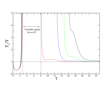
Figure 1: (Color on line) Kinetic temperature $T_{v}$ in the NESS as a function of $\tau$ for $Q_{0}=4$, $g=3.9$, and different values of $n$: $n=25$ (red solid line), $n=50$ (blue), $n=75$ (green), $n=100$ (black), and $n=\infty$ (black dashed line). For $n=25$, the stationary state is stable for $0\leq\tau<2.79$ and $\tau>8.07$. The second stability region is displaced to larger $\tau$ as $n$ increases and no longer exists for $n=\infty$ (discrete delay). In the latter case, the system is stable for $0\leq\tau<\tau_{c,\infty}^{(1)}\simeq 2.53$ only.

Due to the linearity of Eq. (10), the probability distribution function (pdf) in the NESS is a multivariate Gaussian distribution,

$$p({\bf u})=\frac{1}{\sqrt{(2\pi)^{n+2}\det\Sigma}}e^{-\frac{1}{2}{\bf u}^{T}.\Sigma^{-1}.{\bf u}}\ ,$$ (26)

where $\Sigma$, the $(n+2)\times(n+2)$ covariance matrix (not to be confused with the entropy production defined above), is solution of the Lyapunov equation G2004

$$A\Sigma+\Sigma A^{T}=-D\ ,$$ (27)

with $D={\bf d}.{\bf d}^{T}$ has only one non-zero element with ${\bf d}^{T}=(1,0,0...0)$. To solve this equation for large $n$, one can use the property that the eigenvalues of $\Sigma$, ordered as $\lambda_{1}\geq\lambda_{2}\geq...\geq\lambda_{n+2}$, decay very fast as their order increases. Therefore, although $\Sigma$ is full-rank in the stability region, the numerical rank is very low. This feature is commonly encountered in large-scale Lyapunov equations when the matrix in the right-hand side of the equation has a low rank P2000 ; ASZ2002 . Such equations typically arise in the study of the controllability and observability of linear time-invariant (LTI) dynamical systems, with the matrix in the right-hand side having a rank equal to the number of inputs or outputs in the system B2021 . One can then use accurate low-rank approximations to the solution and consider large values of $n$ BS2013 ; S2016 . When extremely high precision is required, one can also use the closed-form expression of $\Sigma$ in terms of the Cauchy matrix built from the eigenvalues of $A$ P2000 ; ASZ2002 ; S2016 .

III Matrix Riccati equations and their properties

III.1 Basic equations

We now come to the heart of the matter and derive the Riccati differential equations (RDEs) that will allow us to investigate the time evolution of the moment generating functions $G_{\rm o,\lambda}(t)\equiv\langle e^{-\lambda{\cal A}_{t}}\rangle$ in the steady state and to extract the complete asymptotic form at large time:

$$G_{\rm o,\lambda}(t)\sim g_{\rm o}(\lambda)e^{\mu_{\rm o}(\lambda)t}\ ,$$ (28)

where

$$\mu_{\rm o}(\lambda)\equiv\lim_{t\to\infty}\frac{1}{t}\ln G_{\rm o,\lambda}(t)$$ (29)

is the SCGF and $g_{\rm o}(\lambda)$ is the pre-exponential factor.

As will be discussed in detail in the following (see Sec. IV.2.1), the domain of definition of the SCGF (i.e., the values of $\lambda$ for which $\mu_{\rm o}(\lambda)<\infty$) may depend on the observable. This is due to rare but large fluctuations of the initial or final points of the stochastic trajectories that induce singularities in the pre-exponential factors. Therefore, the knowledge of both $\mu_{\rm o}(\lambda)$ and $g_{\rm o}(\lambda)$ is required to obtain the large-time behavior of the pdf $P_{\rm o}(a,t)\equiv\langle\delta({\cal A}_{t}-at)\rangle$ characterized by the rate function

$$I_{\rm o}(a)\equiv-\lim_{t\to\infty}\frac{1}{t}\ln P_{\rm o}(a,t)\ .$$ (30)

Large deviation theory tells us that if $\mu_{\rm o}(\lambda)$ exists and is differentiable, then $I_{\rm o}(a)$ is given by the Legendre-Fenchel transform T2009 ; J2020

$$I_{\rm o}(a)=\max_{\lambda}[-\lambda a-\mu_{\rm o}(\lambda]\ .$$ (31)

In order to compute $G_{\rm o,\lambda}(t)$, it is convenient to start from the restricted generating function $G_{\rm o,\lambda}({\bf u},t|{\bf u}_{0})=\langle e^{-\lambda{\cal A}_{t}}\rangle_{{\bf u}_{0},{\bf u}}$, where the initial and final configurations of the trajectories of duration $t$ are fixed at ${\bf u}_{0}$ and ${\bf u}$, respectively. By definition, $G_{\rm o,\lambda}({\bf u},0|{\bf u}_{0})=\delta({\bf u}-{\bf u}_{0})$ and

$$G_{\rm o,\lambda}(t) =\int d{\bf u}_{0}\>p({\bf u}_{0})\int d{\bf u}\>G_{\rm o,\lambda}({\bf u},t|{\bf u}_{0})$$ (32)

provided the integrals over ${\bf u}_{0}$ and ${\bf u}$ converge. This suggests considering the time evolution of

$$G^{r}_{\rm o,\lambda}({\bf u}_{0},t) =\int d{\bf u}\>G_{\rm o,\lambda}({\bf u},t|{\bf u}_{0})$$ (33)

and

$$G^{l}_{\rm o,\lambda}({\bf u},t) =\int d{\bf u}_{0}\>p({\bf u}_{0})G_{\rm o,\lambda}({\bf u},t|{\bf u}_{0})$$ (34)

separately. They satisfy the initial conditions

$$G^{r}_{\rm o,\lambda}({\bf u}_{0},0)=1$$ (35)

and

$$G^{l}_{\rm o,\lambda}({\bf u},0)=p({\bf u})\ .$$ (36)

(The superscript r and l denote “right” and “left”, respectively. This notation will be justified later when considering the long-time limit.)

Standard application of the Feynman-Kac formula (see, e.g., Ref. M2005 for a pedagogical review) shows that $G^{r}_{\rm o,\lambda}({\bf u}_{0},t)$ evolves in time according to the backward Fokker-Planck equation

$$\partial_{t}G^{r}_{\rm o,\lambda}({\bf u}_{0},t)={\cal L}_{\rm o,\lambda}G^{r}_{\rm o,\lambda}({\bf u}_{0},t)\ ,$$ (37)

where ${\cal L}_{\rm o,\lambda}$ is the so-called tilted (or biased) generator given by CT2015 ; T2018

$${\cal L}_{\rm o,\lambda}={\bf F}\cdot({\bf\nabla}-\lambda{\bf g}_{\rm o})+\frac{1}{2}(\nabla-\lambda{\bf g}_{\rm o})\cdot D(\nabla-\lambda{\bf g}_{\rm o})\ ,$$ (38)

with ${\bf F}=A{\bf u}$ in the case at hand. Explicit expressions of ${\cal L}_{\rm o,\lambda}$ for ${\rm o}=w,q,\sigma$ are given in Appendix A. Likewise, $G^{l}_{\rm o,\lambda}({\bf u},t)$ satisfies the forward Fokker-Planck equation

$$\partial_{t}G^{l}_{\rm o,\lambda}({\bf u},t)={\cal L}_{\rm o,\lambda}^{{\dagger}}G^{l}_{\rm o,\lambda}({\bf u},t)\ ,$$ (39)

where ${\cal L}_{\rm o,\lambda}^{\dagger}$ is the adjoint of ${\cal L}_{\rm o,\lambda}$.

Solving such linear partial differential equations beyond the long-time limit requires one to determine the whole spectrum of the operators ${\cal L}_{\rm o,\lambda}$ and ${\cal L}_{\rm o,\lambda}^{\dagger}$ and the associated eigenfunctions, which is a daunting or even impossible task. In the present case, however, both the drift ${\bf F}$ and the vector function ${\bf g}_{\rm o}$ depend linearly on ${\bf u}$ so that we can anticipate that the solutions of Eqs. (37) and (39) with initial conditions (35) and (36), respectively, are just multivariate Gaussians. Specifically, we show in Appendix B.0.1 that

$$G^{r}_{\rm o,\lambda}({\bf u}_{0},t) =\exp\left(-\frac{1}{2}{\bf u}_{0}^{T}C^{r}_{\rm o}(\lambda,t){\bf u}_{0}+\int_{0}^{t}f^{r}_{\rm o}(\lambda,t^{\prime})dt^{\prime}\right)$$ (40a)

$$G^{l}_{\rm o,\lambda}({\bf u},t) =\left[(2\pi)^{n+2}\det\Sigma\right]^{-1/2}\exp\left(-\frac{1}{2}{\bf u}^{T}C^{l}_{\rm o}(\lambda,t){\bf u}+\int_{0}^{t}f^{l}_{\rm o}(\lambda,t^{\prime})dt^{\prime}\right)\ ,$$ (40b)

with

$$f^{r}_{\rm o}(\lambda,t) =-\frac{1}{2}\mbox{Tr}[D(C_{\rm o}^{r}(\lambda,t)+\lambda B_{\rm o})]$$ (41a)

$$f^{l}_{\rm o}(\lambda,t) =-\frac{1}{2}\mbox{Tr}[D(C_{\rm o}^{l}(\lambda,t)-\lambda B_{\rm o})]-\mbox{Tr}(A)\ .$$ (41b)

$C^{r}_{\rm o}(\lambda,t)$ and $C^{l}_{\rm o}(\lambda,t)$ are symmetric matrices of dimension $(n+2)\times(n+2)$ which are solutions of the matrix differential equations

$$\dot{C}_{\rm o}^{r}(\lambda,t) ={\cal R}_{\rm o,\lambda}\big{[}C_{\rm o}^{r}(\lambda,t)\big{]}$$ (42a)

$$\dot{C}_{\rm o}^{l}(\lambda,t) ={\cal R}_{\rm o,\lambda}\big{[}-C_{\rm o}^{l}(\lambda,t)\big{]}$$ (42b)

with initial conditions

$$C_{\rm o}^{r}(\lambda,0) =0$$ (43a)

$$C_{\rm o}^{l}(\lambda,0) =C\ ,$$ (43b)

respectively, where $C$ is the inverse of the covariance matrix $\Sigma$. In these equations, ${\cal R}_{\rm o,\lambda}$ is a quadratic Riccati operator acting on a general $(n+2)\times(n+2)$ matrix $X$ as

$${\cal R}_{\rm o,\lambda}[X]=A_{\rm o}(\lambda)^{T}X+XA_{\rm o}(\lambda)-XDX+K_{\rm o}(\lambda)\ ,$$ (44)

with

$$A_{\rm o}(\lambda)=A-\lambda DB_{\rm o}\ ,$$ (45)

and

$$K_{\rm o}(\lambda)=\lambda(A^{T}B_{\rm o}+B_{\rm o}^{T}A)-\lambda^{2}B^{T}_{\rm o}DB_{\rm o}\ .$$ (46)

The explicit expressions of the symmetric matrices $K_{\rm o}(\lambda)$ are given in Appendix B.0.2. Furthermore, since $D_{ij}=\delta_{i1}\delta_{j1}$ and $\mbox{Tr}(A)=-(1/Q_{0}+n^{2}/\tau)$ in the present model, Eqs. (41) become

$$f^{r}_{\rm o}(\lambda,t) =-\frac{1}{2}(C_{\rm o,11}^{r}(\lambda,t)+\lambda B_{\rm o,11})$$ (47a)

$$f^{l}_{\rm o}(\lambda,t) =-\frac{1}{2}(C_{\rm o,11}^{l}(\lambda,t)-\lambda B_{\rm o,11})+\frac{1}{Q_{0}}+\frac{n^{2}}{\tau}\ .$$ (47b)

By integrating $G^{r}_{\rm o,\lambda}({\bf u}_{0},t)p({\bf u}_{0})$ over ${\bf u}_{0}$ and $G^{l}_{\rm o,\lambda}({\bf u},t)$ over ${\bf u}$, we then obtain two expressions of the generating function $G_{\rm o,\lambda}(t)$,

$$G_{\rm o,\lambda}(t) =\Big{[}\frac{\det\big{(}C^{r}_{\rm o}(\lambda,t)+C\big{)}}{\det C}\Big{]}^{-1/2}\exp\big{(}\int_{0}^{t}f^{r}_{\rm o}(\lambda,t^{\prime})dt^{\prime}\big{)}$$ (48a)

$$=\Big{[}\frac{\det C^{l}_{\rm o}(\lambda,t)}{\det C}\Big{]}^{-1/2}\>\exp\big{(}\int_{0}^{t}f^{l}_{\rm o}(\lambda,t^{\prime})dt^{\prime}\big{)}\ .$$ (48b)

By construction, these two expressions give the same result as long as the solutions of Eqs. (42) exist (see the discussion in the next section). But for the generating function $G_{\rm o,\lambda}(t)$ to be finite it is mandatory that the matrices $C+C_{\rm o}^{r}(\lambda,t)$ and $C_{\rm o}^{l}(\lambda,t)$ are positive definite. As we shall see later in Sec. IV.1, this crucial condition is not always satisfied. Moreover, the equivalence between Eqs. (48a) and (48b) may result from a nontrivial mathematical mechanism.

Finally, let us note that an alternative expression of $G_{\rm o,\lambda}(t)$ is available when the matrix $C_{\rm o}^{l}(\lambda,t^{\prime})$ is invertible for all $t^{\prime}\in[0,t]$. If so, a few manipulations detailed in Appendix B.0.3 lead to

$$G_{\rm o,\lambda}(t) =\exp\left(-\frac{1}{2}\int_{0}^{t}\mbox{Tr}\big{(}K_{\rm o}(\lambda)\Sigma^{l}_{\rm o}(\lambda,t^{\prime})+\lambda DB_{\rm o}\big{)}dt^{\prime}\right)\ ,$$ (49)

where $\Sigma^{l}_{\rm o}(\lambda,t)$, the inverse matrix of $C_{\rm o}^{l}(\lambda,t)$, is solution of the complementary RDE

$$\frac{\partial}{\partial t}\Sigma^{l}_{\rm o}(\lambda,t)=A_{\rm o}(\lambda)\Sigma^{l}_{\rm o}(\lambda,t)+\Sigma^{l}_{\rm o}(\lambda,t)A^{T}_{\rm o}(\lambda)-\Sigma^{l}_{\rm o}(\lambda,t)K_{\rm o}(\lambda)\Sigma^{l}_{\rm o}(\lambda,t)+D\ ,$$ (50)

with initial condition

$$\Sigma^{l}_{\rm o}(\lambda,0)=\Sigma\ .$$ (51)

In particular, using the fact that $B_{q,11}=-2/Q_{0}$ and $K_{q}(1)=0$ [Eq. (B14)], Eq. (49) readily yields

$$G_{q,\lambda=1}(t) =e^{t/Q_{0}}\ ,$$ (52)

which is the universal IFT for the fluctuating heat in underdamped Langevin processes RTM2016 . This result is also directly obtained from Eq. (42a) since the unique solution of the initial value problem is $C^{r}_{q}(\lambda=1,t)=0$, which implies that $f^{r}_{q}(\lambda=1,t)=1/Q_{0}$ from Eq. (47a).

III.2 Properties of the Riccati differential equations (RDEs)

RDEs similar to Eqs. (42), as well as the corresponding continuous algebraic Riccati equations (CAREs) whose solutions are stationary solutions of the RDEs (see Sec. III.3 below), appear in many branches of applied mathematics, the most prominent application being linear optimal control and filtering problems B2021 . Within this framework, several important issues have been extensively discussed in the literature such as the global existence of the solutions as one varies the coefficients of the differential equation or the initial data, the convergence toward a particular solution of the corresponding CARE as $t\to\infty$, and the mechanism of attraction (see Ref. AFIJ2003 and references therein). In particular, it is a standard result that the solution of the RDE (which is unique for a given initial condition) exists for $t\in[0,\infty)$ and is symmetric, positive semidefinite if the source term (in the present case, the matrix $K_{\rm o}(\lambda)$ in Eq. (44)), the quadratic term (i.e., the term $XDX$), and the initial condition are positive semidefinite. With additional conditions on the coefficients, it is also proven that the solution converges monotonically to the maximal solution $X^{+}$ of the CARE (to be defined later) which turns out to be the unique symmetric positive semidefinite solution.

Unfortunately, it is readily seen from Eqs. (B13)-(B15) that neither $K_{w}(\lambda)$ nor $K_{\sigma}(\lambda)$ are positive semidefinite ($n$ eigenvalues are equal to $0$, one is positive, and one is negative). Only $K_{q}(\lambda)\geq 0$ for $0\leq\lambda\leq 1$. This is an essential difference with the standard situation treated in linear quadratic (LQ) optimal control, and it significantly complicates the present study note3 . The consequences that will be explored in the rest of this paper and illustrated numerically are the following:

1) the solutions of Eqs. (42) may exhibit a finite-time escape phenomenon, which means that they may blow up in a finite time,

2) they may fail to converge (i.e., the solution may oscillate),

3) they may converge to a solution of the CARE which is not the maximal solution,

4) the maximal solution is not automatically positive semidefinite.

On the positive side, the Riccati operator defined by Eq. (44) has a remarkable property that holds for arbitrary matrices $A$, $B_{\rm o}$, and $D$ symmetric. Indeed, if $S$ is a symmetric matrix, then

$${\cal R}_{\rm o,\lambda}[X]={\cal R}^{\prime}_{\rm o,\lambda}[X-\lambda S]\ ,$$ (53)

where ${\cal R}^{\prime}_{\rm o,\lambda}$ is the modified operator obtained by changing $B_{\rm o}$ into $B^{\prime}_{\rm o}=B_{\rm o}+S$. Therefore, when the matrices $B_{\rm o}$ characterizing the various observables only differ by their symmetric part $S_{\rm o}$, which is the case for the three observables ${\cal W}_{t},{\cal Q}_{t},\Sigma_{t}$ under consideration, one has

$${\cal R}_{\rm o,\lambda}[X]={\cal R}_{\rm o^{\prime},\lambda}[X+\lambda(S_{\rm o}-S_{\rm o^{\prime}})]\ .$$ (54)

This “invariance” property allows one to compute all matrices $C^{r}_{\rm o^{\prime}}(\lambda,t)$ and $C^{l}_{\rm o^{\prime}}(\lambda,t)$ by solving the RDEs corresponding to a single operator ${\cal R}_{\rm o,\lambda}$ but with different initial conditions. Specifically, by letting $X_{\rm o^{\prime}}(\lambda,t)$ be the solution of the RDE $\dot{X}_{\rm o^{\prime}}={\cal R}_{\rm o,\lambda}[X_{\rm o^{\prime}}]$ with initial condition

$$X_{\rm o^{\prime}}(\lambda,0)=\lambda(S_{\rm o^{\prime}}-S_{\rm o})$$ (55)

we obtain that

$$C^{r}_{\rm o^{\prime}}(\lambda,t)=X_{\rm o^{\prime}}(\lambda,t)-\lambda(S_{\rm o^{\prime}}-S_{\rm o})$$ (56)

and, similarly, if $X_{\rm o^{\prime}}(\lambda,t)$ is the solution of the RDE $\dot{X}_{\rm o^{\prime}}={\cal R}_{\rm o,\lambda}[-X_{\rm o^{\prime}}]$ with initial condition

$$X_{\rm o^{\prime}}(\lambda,0)=C-\lambda(S_{\rm o^{\prime}}-S_{\rm o})$$ (57)

we have that

$$C^{l}_{\rm o^{\prime}}(\lambda,t)=X_{\rm o^{\prime}}(\lambda,t)+\lambda(S_{\rm o^{\prime}}-S_{\rm o}).$$ (58)

III.2.1 Global existence of the solutions

We begin our study of the solutions of the RDEs (42) by briefly discussing the issue of their global existence. First of all, we note that the non-negativity of the diffusion matrix $D$ implies that the solutions are bounded from above by the solutions of the corresponding Lyapunov differential equations (i.e., Eqs. (42) with $D=0$) note4 . Since these upper bounds do not blow up in finite time, the finite-time escape phenomenon, when it occurs, is due to the absence of a lower bound and manifests itself by the divergence of the smallest eigenvalue of $C^{r}_{\rm o}(\lambda,t)$ or $C^{l}_{\rm o}(\lambda,t)$ toward $-\infty$. This is a crucial observation because it means that this eigenvalue, which is initially positive (as $C+C^{r}_{\rm o}(\lambda,0)=C^{l}_{\rm o}(\lambda,0)=C$), vanishes before diverging to $-\infty$. Therefore, this finite-time escape phenomenon is always preceded by the divergence of the generating function $G_{\rm o,\lambda}(t)$.

Let us focus on the case $0\leq\lambda\leq 1$ for which we can take advantage of the semi-positiveness of the source term $K_{q}(\lambda)$ to draw definite conclusions about the global existence of the solutions of the RDEs and of the generating function. It suffices to consider the “right” matrices $C^{r}_{\rm o}(\lambda,t)$ since the condition $C+C^{r}_{\rm o}(\lambda,t)>0$ for all $t\in[0,\infty)$ implies that $C^{l}_{\rm o}(\lambda,t)>0$ (otherwise, the two expressions (48a) and (48b) of $G_{\rm o,\lambda}(t)$ would not be consistent).

First of all, since $C^{r}_{q}(\lambda,0)=0$ and the RDE $\dot{X}={\cal R}_{q,\lambda}[X]$ has all the properties of the RDEs encountered in LQ optimal control AFIJ2003 , we can immediately assert that the matrix $C^{r}_{q}(\lambda,t)$ exists and is positive semidefinite on $[0,\infty)$. Moreover, $\dot{C}^{r}_{q}(\lambda,0)=K_{q}(\lambda)\geq 0$ and thus $C^{r}_{q}(\lambda,t)$ is monotonically non-decreasing note80 . Hence $C^{r}_{q}(\lambda,t)+C>0$ and we conclude that the generating function $G_{q,\lambda}(t)$ is always finite.

Reaching a conclusion about the existence and positiveness of the matrices $C+C^{r}_{w}(\lambda,t)$ and $C+C^{r}_{\sigma}(\lambda,t)$ is less straightforward. We first note from Eqs. (22) and (23) that $S_{q}\leq 0$ and $S_{\sigma}-S_{q}\geq 0$. We then exploit the order-preserving property of Riccati differential equations which states that the solutions depend monotonically on the initial values note8 . Accordingly, the solutions $X_{w}(\lambda,t)$ and $X_{\sigma}(\lambda,t)$ of the RDE $\dot{X}={\cal R}_{q,\lambda}[X]$, which correspond respectively to the initial conditions $X_{w}(\lambda,0)=-\lambda S_{q}\geq 0$ and $X_{\sigma}(\lambda,0)=\lambda(S_{\sigma}-S_{q})\geq 0$, satisfy $X_{w}(\lambda,t)\geq C^{r}_{q}(\lambda,t)$ and $X_{\sigma}(\lambda,t)\geq C^{r}_{q}(\lambda,t)$. From the “invariance” relations (56) and (58) (with $S_{w}=0$) we then obtain

$$C_{w}^{r}(\lambda,t)=X_{w}(\lambda,t)+\lambda S_{q}\geq C^{r}_{q}(\lambda,t)+\lambda S_{q}$$ (59)

and

$$C_{\sigma}^{r}(\lambda,t)=X_{\sigma}(\lambda,t)-\lambda(S_{\sigma}-S_{q})\geq C^{r}_{q}(\lambda,t)-\lambda(S_{\sigma}-S_{q})\ .$$ (60)

Furthermore, it can be shown that

$$\det[C+\lambda S_{q}] =\det[I_{n+2}+\lambda S_{q}\Sigma]\>\det C=(1-\lambda\frac{T_{v}}{T})(1-\lambda\frac{T_{x}}{T})\>\det C$$ (61)

and

$$\det[C+\lambda(S_{q}-S_{\sigma})]=(1-\lambda)^{2}\>\det C\ .$$ (62)

As a result, $C+\lambda S_{q}>0$ for $\lambda<\min(T/T_{x},T/T_{v})$ and $C+\lambda(S_{q}-S_{\sigma})>0$ for $\lambda<1$ (since all eigenvalues of these matrices are positive for $\lambda=0$ and remain positive as long as the respective determinants do not vanish). From this set of inequalities we conclude that

$$C^{r}_{w}(\lambda,t)+C\geq C^{r}_{q}(\lambda,t)+C+\lambda S_{q}>0\ ,\>\>0\leq\lambda<\min(1,T/T_{x},T/T_{v})$$ (63)

and

$$C^{r}_{\sigma}(\lambda,t)+C\geq C^{r}_{q}(\lambda,t)+C-\lambda(S_{\sigma}-S_{q})>0\ ,\>\>0\leq\lambda<1\ .$$ (64)

In consequence, the corresponding generating functions $G_{w,\lambda}(t)$ and $G_{\sigma,\lambda}(t)$ are always finite for values of $\lambda$ within the above ranges. We stress that these conditions are sufficient but not necessary. Note also that the inequality (63) still holds for $\lambda=1$ if both $T_{x}$ and $T_{v}$ are smaller than $T$. On the other hand, the strict inequality (64) is replaced by $C^{r}_{\sigma}(1,t)+C\geq 0$. This special but important case $\lambda=1$ will be treated in detail in Sec. V.

III.2.2 Solutions of the RDEs and asymptotic behavior

Various methods for solving RDEs are available in the literature, including for large-scale problems BM2004 . Here, we will use the classical approach that consists in transforming each quadratic differential equation into a linear system of first-order Hamiltonian differential equations of double size AFIJ2003 . We can then obtain a closed-form representation of the solution which is suitable for analyzing the asymptotic behavior and the dependence on the initial condition. Although this procedure is standard, it is worthwhile to replicate the derivation in the case at hand.

Consider first Eq. (42a) with initial condition (43a). It can be checked by direct substitution that the solution can be expressed as

$$C^{r}_{{\rm o}}(\lambda,t) =V^{r}_{\rm o}(\lambda,t)U^{r}_{\rm o}(\lambda,t)^{-1}\ ,$$ (65)

where the matrices $U^{r}_{\rm o}(\lambda,t)$ and $V^{r}_{\rm o}(\lambda,t)$ are solutions of the linear system

$$\begin{bmatrix}\dot{U}^{r}_{\rm o}(\lambda,t)\\ \dot{V}^{r}_{\rm o}(\lambda,t)\end{bmatrix}=H_{\rm o}^{r}(\lambda)\begin{bmatrix}U^{r}_{\rm o}(\lambda,t)\\ V^{r}_{\rm o}(\lambda,t)\end{bmatrix}\ ,$$ (66)

with

$$H_{\rm o}^{r}(\lambda)=\begin{bmatrix}-A_{\rm o}(\lambda)&D\\ K_{\rm o}(\lambda)&A_{\rm o}^{T}(\lambda)&\end{bmatrix}\ ,$$ (67)

and initial condition

$$\begin{bmatrix}U^{r}_{\rm o}(\lambda,0)\\ V^{r}_{\rm o}(\lambda,0)\end{bmatrix} =\begin{bmatrix}I_{n+2}\\ 0\end{bmatrix}\ .$$ (68)

As a consequence,

$$\begin{bmatrix}U^{r}_{\rm o}(\lambda,t)\\ V^{r}_{\rm o}(\lambda,t)\end{bmatrix}=e^{H^{r}_{\rm o}(\lambda)t}\begin{bmatrix}I_{n+2}\\ 0\end{bmatrix}\ .$$ (69)

The existence of the solution of Eq. (42a) for all $t^{\prime}\in[0,t]$ ensures that the corresponding matrix $U^{r}_{\rm o}(\lambda,t^{\prime})$ is invertible in this interval. Conversely, if $U^{r}_{\rm o}(\lambda,t^{\prime})$ is nonsingular for all $t^{\prime}\in[0,t]$, then $C^{r}_{\rm o}(\lambda,t^{\prime})$ exists in the same interval and is given by Eq. (65).

A similar transformation holds for the solution $C^{l}_{\rm o}(\lambda,t)$ of Eq. (42b), with $U^{r}_{\rm o}(\lambda,t),V^{r}_{\rm o}(\lambda,t)$ replaced by $U^{l}_{\rm o}(\lambda,t),V^{l}_{\rm o}(\lambda,t)$ and Eqs. (69) replaced by

$$\begin{bmatrix}U^{l}_{\rm o}(\lambda,t)\\ V^{l}_{\rm o}(\lambda,t)\end{bmatrix}=e^{H^{l}_{\rm o}(\lambda)t}\begin{bmatrix}I_{n+2}\\ C\end{bmatrix}\ .$$ (70)

with

$$H^{l}_{\rm o}(\lambda)=\begin{bmatrix}A_{\rm o}(\lambda)&D\\ K_{\rm o}(\lambda)&-A_{\rm o}^{T}(\lambda)&\end{bmatrix}\ .$$ (71)

The $2(n+2)\times 2(n+2)$ matrices $H^{r}_{\rm o}(\lambda)$ and $H^{l}_{\rm o}(\lambda)$ are Hamiltonian matrices which play a central role in the forthcoming analysis. Their spectral properties are investigated in Appendix C. Observe in particular that $H^{r}_{\rm o}(\lambda)$ and $H^{l}_{\rm o}(\lambda)$ are invertible and that the eigenvalue spectrum only depends on the anti-symmetric part of the matrices $B_{\rm o}$ (a property that is shared by all linear current-type observables). In the present case, the anti-symmetric part is the same for the three observables [Eq. (20)], and owing to the fact that $D_{ij}=\delta_{1i}\delta_{1j}$, the characteristic polynomial of the Hamiltonian matrices is shown in Appendix C.0.1 to be given by

$$(-1)^{n}p_{H}(\lambda,s)=p_{A}(s)p_{A}(-s)-\frac{2\lambda g}{Q_{0}^{2}}(\frac{n}{\tau})^{2n}\>s[(1-\frac{s\tau}{n})^{n}-(1+\frac{s\tau}{n})^{n}]\ ,$$ (72)

where $p_{A}(s)$, the characteristic polynomial of $A$, is given by Eq. (24).

For the sake of simplicity, we will assume in the following that the matrices $H^{r}_{\rm o}(\lambda)$ and $H^{l}_{\rm o}(\lambda)$ are diagonalizable. This is not an essential assumption but it simplifies the presentation as we can then avoid to deal with the more complicated Jordan forms of the Hamiltonian matrices AFIJ2003 . More important is the fact that the values of $\lambda$ will be restricted to a certain open interval ${\cal D}_{H}=(\lambda_{\min},\lambda_{\max})$ for which $H^{r}_{\rm o}(\lambda)$ and $H^{l}_{\rm o}(\lambda)$ have no purely imaginary eigenvalues. As will be shown in Sec. IV.2.3, this restriction is justified by the fact that the values of $\lambda$ outside ${\cal D}_{H}$ are irrelevant for the determination of the rate function $I(a)$.

The condition $\lambda\in{\cal D}_{H}$ has two significant consequences:

$\bullet$ The Hamiltonian matrices are dichotomically separable AFIJ2003 , with $n+2$ eigenvalues $s^{+}_{1}(\lambda),s^{+}_{2}(\lambda),...s^{+}_{n+2}(\lambda)$ having a positive real part and $n+2$ eigenvalues $s_{1}^{-}(\lambda)=-s_{1}^{+}(\lambda),s_{2}^{-}(\lambda)=-s_{2}^{+}(\lambda),...s_{n+2}^{-}(\lambda)=-s^{+}_{n+2}(\lambda)$ having a negative real part (the eigenvalues are counted with their multiplicities and the ordering is arbitrary unless otherwise specified).

$\bullet$ Exact mathematical statements ensure that the corresponding algebraic Riccati equations have real symmetric solutions (see the discussion in the next section).

Let us consider the matrix $H_{\rm o}^{r}(\lambda)$. As a result of the above assumptions, we can introduce a basis-change matrix $W^{r}_{\rm o}(\lambda)$ that diagonalizes $H_{\rm o}^{r}(\lambda)$ such that

$$H_{\rm o}^{r}(\lambda)=W^{r}_{\rm o}(\lambda)\ \begin{bmatrix}J(\lambda)&0\\ 0&-J(\lambda)&\end{bmatrix}[W^{r}_{\rm o}(\lambda)]^{-1}\ ,$$ (73)

where $J(\lambda)=\mbox{diag}\big{(}s^{+}_{1}(\lambda),s^{+}_{2}(\lambda),...s^{+}_{n+2}(\lambda)\big{)}$. Eq. (69) then becomes

$$\begin{bmatrix}U^{r}_{\rm o}(\lambda,t)\\ V^{r}_{\rm o}(\lambda,t)\end{bmatrix}=W^{r}_{\rm o}(\lambda)\begin{bmatrix}e^{J(\lambda)t}&0\\ 0&e^{-J(\lambda)t}&\end{bmatrix}[W^{r}_{\rm o}(\lambda)]^{-1}\begin{bmatrix}I_{n+2}\\ 0\end{bmatrix}\ .$$ (74)

We next partition the matrix $W^{r}_{\rm o}(\lambda)$ into $4$ blocks of size $(n+2)\times(n+2)$,

$$W^{r}_{\rm o}(\lambda)=\begin{bmatrix}W^{r,11}_{\rm o}(\lambda)&W^{r,12}_{\rm o}(\lambda)\\ W^{r,21}_{\rm o}(\lambda)&W^{r,22}_{\rm o}(\lambda)&\end{bmatrix}\ ,$$ (75)

where the first $n+2$ columns are the eigenvectors relative to the eigenvalues $s_{i}^{+}(\lambda)$ and the remaining columns are the eigenvectors relative to the eigenvalues $s_{i}^{-}(\lambda)$.

Now, suppose that the submatrix $W^{r,22}_{\rm o}(\lambda)$ is nonsingular, so that the matrix

$$T^{r}_{\rm o}(\lambda)= -[W^{r,22}_{\rm o}(\lambda)]^{-1}W^{r,21}_{\rm o}(\lambda)$$ (76)

exists. Simple manipulations, similar to those performed in Refs. K1973 ; FJ1996 and detailed in Appendix D, then lead to a representation of the solution of the RDE (42a) that only involves negative exponentials:

$$C^{r}_{\rm o}(\lambda,t) =[W^{r,21}_{\rm o}(\lambda)+W^{r,22}_{\rm o}(\lambda)P^{r}_{\rm o}(\lambda,t)][W^{r,11}_{\rm o}(\lambda)+W^{r,12}_{\rm o}(\lambda)P^{r}_{\rm o}(\lambda,t)]^{-1}\ ,$$ (77)

where

$$P^{r}_{\rm o}(\lambda,t)=e^{-J(\lambda)t}T^{r}_{\rm o}(\lambda)e^{-J(\lambda)t}\ .$$ (78)

Two important features of the solution are revealed by Eq. (77):

$\bullet$ $C^{r}_{\rm o}(\lambda,t)$ diverges at time $t$ if the matrix $W^{r,11}_{\rm o}(\lambda)+W^{r,12}_{\rm o}(\lambda)P^{r}_{\rm o}(\lambda,t)$ is singular. Finite-time singularities in the solution are thus poles corresponding to $\det[W^{r,11}_{\rm o}(\lambda)+W^{r,12}_{\rm o}(\lambda)P^{r}_{\rm o}(\lambda,t)]=0$. (We recall that the generating function $G_{\rm o,\lambda}(t)$ diverges before the solution or the RDE blows up.)

$\bullet$ $C^{r}_{\rm o}(\lambda,t)$ converges towards the matrix $\hat{C}^{r,+}_{\rm o}(\lambda)\equiv W^{r,21}_{\rm o}(\lambda)[W^{r,11}_{\rm o}(\lambda)]^{-1}$ as $t\to\infty$. (This is true even if finite-time singularities are present.)

As will be shown in the next subsection, $\hat{C}^{r,+}_{\rm o}(\lambda)$ is the so-called “maximal” (real symmetric) solution of the corresponding algebraic equation (86a) and its existence is certified LR1995 (which means that the matrix $W^{r,11}_{\rm o}(\lambda)$ is nonsingular). On the other hand, the assumption that $W^{r,22}_{\rm o}(\lambda)$ is nonsingular, which is required for Eq. (77) to be meaningful, may not be satisfied for some values of $\lambda$. In other words, the condition $\det W^{r,22}_{\rm o}(\lambda)\neq 0$ ensures that the initial matrix $C^{r}_{\rm o}(\lambda,0)=0$ belongs to the basin of attraction of $\hat{C}^{r,+}_{\rm o}(\lambda)$. Otherwise, Eq. (77) is no longer valid and the solution of the RDE (42a) goes to another limit or may fail to converge (i.e., oscillates), as will be discussed in Sec. IV.3.2.

Likewise, the solution of Eq. (42b) can be represented as

$$C^{l}_{\rm o}(\lambda,t) =[W^{l,21}_{\rm o}(\lambda)+W^{l,22}_{\rm o}(\lambda)P^{l}_{\rm o}(\lambda,t)][W^{l,11}_{\rm o}(\lambda)+W^{l,12}_{\rm o}(\lambda)P^{l}_{\rm o}(\lambda,t)]^{-1}\ ,$$ (79)

where

$$P^{l}_{\rm o}(\lambda,t)=e^{-J(\lambda)t}T^{l}_{\rm o}(\lambda)e^{-J(\lambda)t}\ ,$$ (80)

and

$$T^{l}_{\rm o}(\lambda)= -[W^{l,22}_{\rm o}(\lambda)-CW^{l,12}_{\rm o}(\lambda)]^{-1}[W^{l,21}_{\rm o}(\lambda)-CW^{l,11}_{\rm o}(\lambda)]\ .$$ (81)

This requires that the matrix $W^{l,22}_{\rm o}(\lambda)-CW^{l,12}_{\rm o}(\lambda)$ is nonsingular. If true, $C^{l}_{\rm o}(\lambda,t)$ converges asymptotically toward the matrix $\hat{C}^{l,+}_{\rm o}(\lambda)\equiv W^{l,21}_{\rm o}(\lambda)[W^{l,11}_{\rm o}(\lambda)]^{-1}$ which is the maximal (real symmetric) solution of the corresponding CARE and whose existence is also guaranteed (implying that $W^{l,11}_{\rm o}(\lambda)$ is nonsingular). Moreover, it is easily seen from the structure of the Hamiltonian matrices $H_{\rm o}^{r}(\lambda)$ and $H_{\rm o}^{l}(\lambda)$ that

$$\begin{bmatrix}W_{\rm o}^{l,11}&W_{\rm o}^{l,12}\\ W_{\rm o}^{l,21}&W_{\rm o}^{l,22}&\end{bmatrix}=\begin{bmatrix}-W_{\rm o}^{r,12}&-W_{\rm o}^{r,11}\\ W_{\rm o}^{r,22}&W_{\rm o}^{r,21}&\end{bmatrix}\ .$$ (82)

As a result, $\hat{C}^{l,+}_{\rm o}(\lambda)=-W^{r,22}_{\rm o}(\lambda)[W^{r,12}_{\rm o}(\lambda)]^{-1}$.

For future reference, it is instructive to rewrite the conditions of convergence towards $\hat{C}^{r,+}_{\rm o}(\lambda)$ and $\hat{C}^{l,+}_{\rm o}(\lambda)$ as

$$\det W^{r,22}_{\rm o}(\lambda) =\det W^{l,21}_{\rm o}(\lambda)=\det\hat{C}^{l,+}_{\rm o}(\lambda)\>\det W^{l,11}_{\rm o}(\lambda)\neq 0\ ,$$ (83)

and

$$\det[W^{l,22}_{\rm o}(\lambda)-CW^{l,12}_{\rm o}(\lambda)]=\det[W^{r,21}_{\rm o}(\lambda)+CW^{r,11}_{\rm o}(\lambda)]=\det[\hat{C}^{r,+}_{\rm o}(\lambda)+C]\det W^{r,11}_{\rm o}(\lambda)\neq 0\ .$$ (84)

As $\det W^{l,11}_{\rm o}(\lambda)$ and $\det W^{r,11}_{\rm o}(\lambda)$ are $\neq 0$, this implies the following equivalences:

$$\det\hat{C}^{l,+}_{\rm o}(\lambda)\neq 0\>\>\Leftrightarrow\>\>C^{r}_{\rm o}(\lambda,t)\to\hat{C}_{\rm o}^{r,+}(\lambda)$$ (85a)

$$\det[\hat{C}^{r,+}_{\rm o}(\lambda)+C]\neq 0\>\>\Leftrightarrow\>\>C^{l}_{\rm o}(\lambda,t)\to\hat{C}_{\rm o}^{l,+}(\lambda)$$ (85b)

These dual relations will be used again and again in the following. They are one of the main reasons for which it is fruitful to study the generating functions $G^{r}_{\rm o,\lambda}({\bf u}_{0},t)$ and $G^{l}_{\rm o,\lambda}({\bf u},t)$ together.

Finally, we stress that the representations (77) and (79) of the solutions of the RDEs (42) not only reveal the most significant features of the solutions but are also useful for numerical calculations. Indeed, as shown in Appendix C.0.2, we have explicit expressions of the basis-change matrices $W^{r}_{w}(\lambda)$ and $W^{l}_{w}(\lambda)$ as a function of the eigenvalues of the Hamiltonian matrices. We can then only consider the RDE corresponding the operator ${\cal R}_{w,\lambda}$ and compute all matrices $C^{r}_{\rm o}(\lambda,t)$ and $C^{l}_{\rm o}(\lambda,t)$ by changing the initial conditions and using relations (56) and (58).

III.3 Fixed points of the Riccati flows

How does one know that the matrices $\hat{C}^{r,+}_{\rm o}(\lambda)$ and $\hat{C}^{l,+}_{\rm o}(\lambda)$ exist and what are their properties? To answer these questions, we now consider the stationary versions of the RDEs (42),

$${\cal R}_{\rm o,\lambda}[\hat{C}^{r}_{\rm o}(\lambda)]=0$$ (86a)

$${\cal R}_{\rm o,\lambda}[-\hat{C}^{l}_{\rm o}(\lambda)]=0\ ,$$ (86b)

which are referred to as continuous-time algebraic Riccati equations (CAREs) in the context of optimal control. These equations may have no solutions at all or multiple solutions, including complex and non-symmetric ones, and we first recall how these solutions, in particular real symmetric ones, can be built.

It is known that there is a one-to-one correspondence between the solutions of a CARE and certain invariant subspaces of the associated Hamiltonian matrix (see Refs. BLW1991 ; LR1995 ; BIM2012 for reviews). Let us consider for instance Eq. (86a) and denote a solution by $\hat{C}^{r,(\alpha)}_{\rm o}(\lambda)$ (then $-\hat{C}^{r,(\alpha)}_{\rm o}(\lambda)$ is a solution of Eq. (86b)). A direct calculation yields

$$H^{r}_{\rm o}(\lambda)\begin{bmatrix}I_{n+2}\\ \hat{C}^{r,(\alpha)}_{\rm o}(\lambda)&\end{bmatrix}=\begin{bmatrix}I_{n+2}\\ \hat{C}^{r,(\alpha)}_{\rm o}(\lambda)&\end{bmatrix}[-A_{\rm o}(\lambda)+D\hat{C}^{r,(\alpha)}_{\rm o}(\lambda)]\ ,$$ (87)

which shows that the columns of the matrix $\left[\begin{smallmatrix}I_{n+2}\\ \hat{C}^{r,(\alpha)}_{\rm o}(\lambda)&\end{smallmatrix}\right]$ span a graph invariant subspace of $H^{r}_{\rm o}(\lambda)$ and the eigenvalues of $-A_{\rm o}(\lambda)+D\hat{C}^{r,(\alpha)}_{\rm o}(\lambda)$ are a subset of the eigenvalues of $H^{r}_{\rm o}(\lambda)$. This simple fact leads to the following characterization of the solutions note20 : Each solution $\hat{C}^{r,(\alpha)}_{\rm o}(\lambda)$ corresponds to a set ${\cal S}_{\lambda}^{(\alpha)}$ of $n+2$ eigenvalues $s_{\alpha_{1}},s_{\alpha_{2}},...s_{\alpha_{n+2}}$ of $H^{r}_{\rm o}(\lambda)$ [specifically, the eigenvalues of $-A_{\rm o}(\lambda)+D\hat{C}^{r,(\alpha)}_{\rm o}(\lambda)$] and $n+2$ associated eigenvectors ${\bf e}^{r}_{\alpha_{j}}=\left[\begin{smallmatrix}{\bf y}^{r}_{\alpha_{j}}\\ {\bf z}^{r}_{\alpha_{j}}\end{smallmatrix}\right]$ (with ${\bf y}^{r}_{\alpha_{j}},{\bf z}^{r}_{\alpha_{j}}\in\mathbb{C}^{n+2}$), such that

$$\hat{C}^{r,(\alpha)}_{\rm o}(\lambda)=Z^{r,(\alpha)}_{\rm o}(\lambda)[Y^{r,(\alpha)}_{\rm o}(\lambda)]^{-1}\ ,$$ (88)

where $Y^{r,(\alpha)}_{\rm o}(\lambda)=[{\bf y}^{r}_{\alpha_{1}},{\bf y}^{r}_{\alpha_{2}},...{\bf y}^{r}_{\alpha_{n+2}}]$ and $Z^{r,(\alpha)}_{\rm o}(\lambda)=[{\bf z}^{r}_{\alpha_{1}},{\bf z}^{r}_{\alpha_{2}},...{\bf z}^{r}_{\alpha_{n+2}}]$. The invertibility of the $(n+2)\times(n+2)$ matrix $Y^{r,(\alpha)}_{\rm o}(\lambda)$ is the condition ensuring that the solution $\hat{C}^{r,(\alpha)}_{\rm o}(\lambda)$ exists, and conversely. The solutions of Eq. (86b) can be characterized in the same manner, with the index $r$ replaced by $l$ and $A_{\rm o}(\lambda)$ replaced by $-A_{\rm o}(\lambda)$ in Eq. (87). (Recall that $H_{\rm o}^{r}(\lambda)$ and $H_{\rm o}^{r}(\lambda)$ have the same eigenvalue spectrum so that $\hat{C}^{r,(\alpha)}_{\rm o}(\lambda)$ and $\hat{C}^{l,(\alpha)}_{\rm o}(\lambda)$ correspond to the same subset ${\cal S}_{\lambda}^{(\alpha)}$ of eigenvalues of $H_{\rm o}^{r}(\lambda)$ and $H_{\rm o}^{l}(\lambda)$.)

Interestingly, the solutions of Eqs. (86) for an observable $\rm o$’ can be readily obtained from the solutions for the observable $\rm o$. This results from the invariance property (54) of the Riccati operator ${\cal R}_{\rm o,\lambda}$, which yields

$$\hat{C}^{r,(\alpha)}_{\rm o^{\prime}}(\lambda)=\hat{C}^{r,(\alpha)}_{\rm o}(\lambda)+\lambda(S_{\rm o}-S_{\rm o^{\prime}})=\hat{C}^{r,(\alpha)}_{\rm o}(\lambda)+\lambda(B_{\rm o}-B_{\rm o^{\prime}})$$ (89a)

$$\hat{C}^{l,(\alpha)}_{\rm o^{\prime}}(\lambda)=\hat{C}^{l,(\alpha)}_{\rm o}(\lambda)-\lambda(S_{\rm o}-S_{\rm o^{\prime}})=\hat{C}^{l,(\alpha)}_{\rm o}(\lambda)-\lambda(B_{\rm o}-B_{\rm o^{\prime}})\ .$$ (89b)

As a result,

$$\hat{C}^{r,(\alpha)}_{\rm o^{\prime}}(\lambda)+\hat{C}^{l,(\alpha)}_{\rm o^{\prime}}(\lambda)=\hat{C}^{r,(\alpha)}_{\rm o}(\lambda)+\hat{C}^{l,(\alpha)}_{\rm o}(\lambda)\ .$$ (90)

Note that $\hat{C}^{r,(\alpha)}_{\rm o^{\prime}}(\lambda)$ and $\hat{C}^{l,(\alpha)}_{\rm o^{\prime}}(\lambda)$ correspond to the same set ${\cal S}_{\lambda}^{(\alpha)}$ of eigenvalues as $\hat{C}^{r,(\alpha)}_{\rm o}(\lambda)$ and $\hat{C}^{l,(\alpha)}_{\rm o}(\lambda)$, which is the set of eigenvalues of the matrices $-A_{\rm o}(\lambda)+D\hat{C}^{r,(\alpha)}_{\rm o}(\lambda)$ and $A_{\rm o}(\lambda)+D\hat{C}^{l,(\alpha)}_{\rm o}(\lambda)$. Indeed, from the definition of $A_{\rm o}(\lambda)$ [Eq. (45)], one has

$$-A_{\rm o}(\lambda)+D\hat{C}^{r,(\alpha)}_{\rm o}(\lambda) =-A+\lambda DB_{\rm o}+D[\hat{C}^{r,(\alpha)}_{\rm o^{\prime}}(\lambda)-\lambda(B_{\rm o}-B_{\rm o^{\prime}}]=-A_{\rm o^{\prime}}(\lambda)+D\hat{C}^{r,(\alpha)}_{\rm o^{\prime}}(\lambda)$$ (91a)

$$A_{\rm o}(\lambda)+D\hat{C}^{l,(\alpha)}_{\rm o}(\lambda) =A-\lambda DB_{\rm o}+D[\hat{C}^{l,(\alpha)}_{\rm o^{\prime}}(\lambda)+\lambda(B_{\rm o}-B_{\rm o^{\prime}})]=A_{\rm o^{\prime}}(\lambda)+D\hat{C}^{l,(\alpha)}_{\rm o^{\prime}}(\lambda)\ .$$ (91b)

Another interesting consequence of Eqs. (89) is that

$$\hat{C}^{r,(\alpha)}_{\rm o}(\lambda) =\hat{C}^{r,(\alpha)}_{\rm o,antisym}(\lambda)-\lambda B_{\rm o,sym}$$ (92a)

$$\hat{C}^{l,(\alpha)}_{\rm o}(\lambda) =\hat{C}^{l,(\alpha)}_{\rm o,antisym}(\lambda)+\lambda B_{\rm o,sym}\ ,$$ (92b)

where $B_{\rm o,sym}\equiv(B_{\rm o}+B^{T}_{\rm o})/2$ is the symmetric part of the matrix $B_{\rm o}$ and $\hat{C}^{r,(\alpha)}_{\rm o,antisym}(\lambda)$ and $\hat{C}^{l,(\alpha)}_{\rm o,antisym}(\lambda)$ are the solutions of the CAREs (86) associated with $B_{\rm o,antisym}\equiv(B_{\rm o}-B^{T}_{\rm o})/2$. Consequently,

$$\hat{C}^{r,(\alpha)}_{\rm o}(\lambda)+\hat{C}^{l,(\alpha)}_{\rm o}(\lambda)=\hat{C}^{r,(\alpha)}_{\rm o,antisym}(\lambda)+\hat{C}^{l,(\alpha)}_{\rm o,antisym}(\lambda)\ .$$ (93)

In accordance with Eqs. (41), we associate to each solutions $\hat{C}^{r,(\alpha)}_{\rm o}(\lambda)$ and $\hat{C}^{l,(\alpha)}_{\rm o}(\lambda)$ of the CAREs (86) the scalar functions

$$f^{r,(\alpha)}_{\rm o}(\lambda) =-\frac{1}{2}\mbox{Tr}[D(\hat{C}^{r,(\alpha)}_{\rm o}(\lambda)+\lambda B_{\rm o})]$$ (94a)

$$f^{l,(\alpha)}_{\rm o}(\lambda) =-\frac{1}{2}\mbox{Tr}[D(\hat{C}^{l,(\alpha)}_{\rm o}(\lambda)-\lambda B_{\rm o})]-\mbox{Tr}(A)\ .$$ (94b)

These two functions are actually equal and independent of the observables. This follows from the fact that ${\cal S}_{\lambda}^{(\alpha)}=\{s_{\alpha_{i}}\}_{i=1}^{n+2}$ is the spectrum of both $-A_{\rm o}(\lambda)+D\hat{C}^{r,(\alpha)}_{\rm o}(\lambda)$ and $A_{\rm o}(\lambda)+D\hat{C}^{l,(\alpha)}_{\rm o}(\lambda)$, whatever $\rm o$, as we just noticed. As a consequence,

$$\sum_{i=1}^{n+2}s_{\alpha_{i}}(\lambda) =\mbox{Tr}[-A_{\rm o}(\lambda)+D\hat{C}^{r,(\alpha)}_{\rm o}(\lambda)]=\mbox{Tr}[A_{\rm o}(\lambda)+D\hat{C}^{l,(\alpha)}_{\rm o}(\lambda)]\ .$$ (95)

Using the definition of $A_{\rm o}(\lambda)$ [Eq. (45)], this yields $f^{r,(\alpha)}_{\rm o}(\lambda)=f^{l,(\alpha)}_{\rm o}(\lambda)=f^{(\alpha)}(\lambda)$ with

$$f^{(\alpha)}(\lambda)=-\frac{1}{2}[\mbox{Tr}(A)+\sum_{i=1}^{n+2}s_{\alpha_{i}}(\lambda)]\ .$$ (96)

So far, we have considered all solutions of Eq. (86) (assuming that they exist). However, in the present context we are only interested in real symmetric solutions. It turns out that the existence of such solutions is ensured due to the following two properties of the matrices involved in the Riccati operator ${\cal R}_{\rm o,\lambda}$ defined by Eq. (44) note6 :

i) the matrix $D$ is positive semidefinite,

ii) the pair of matrices $(A_{\rm o}(\lambda),D)$ is controllable.

These properties also ensure that note7 :

$\bullet$ Each real symmetric solution $\hat{C}^{r,(\alpha)}_{\rm o}(\lambda)$ or $\hat{C}^{l,(\alpha)}_{\rm o}(\lambda)$ corresponds to a set ${\cal S}^{(\alpha)}_{\lambda}$ of eigenvalues of $H^{r}_{\rm o}(\lambda)$ and $H^{l}_{\rm o}(\lambda)$ such that $s\in{\cal S}^{(\alpha)}_{\lambda}$ implies $\bar{s}\in{\cal S}^{(\alpha)}_{\lambda}$ and $-\bar{s}\notin{\cal S}^{(\alpha)}_{\lambda}$.

$\bullet$ The matrices $\hat{C}^{r,+}_{\rm o}(\lambda)=W^{r,21}_{\rm o}(\lambda)[W^{r,11}_{\rm o}(\lambda)]^{-1}$ and $\hat{C}^{l,+}_{\rm o}(\lambda)=W^{l,21}_{\rm o}(\lambda)[W^{l,11}_{\rm o}(\lambda)]^{-1}$ introduced previously exist and are the maximal real symmetric solutions of Eqs. (86a) and (86b) with respect to the positive definiteness ordering. They are obtained by taking ${\cal S}^{(\alpha)}_{\lambda}$ to be the set ${\cal S}_{\lambda}^{+}=\{s^{+}_{1},s^{+}_{2},...s^{+}_{n+2}\}$ of eigenvalues with a positive real part (see the partitioning of the basis change matrices $W^{r}_{\rm o}(\lambda)$ and $W^{l}_{\rm o}(\lambda)$). Likewise, the matrices $C^{r,-}_{\rm o}(\lambda)=W_{\rm o}^{r,22}(\lambda)[W_{\rm o}^{r,12}(\lambda)]^{-1}$ and $C^{l,-}_{\rm o}(\lambda)=W_{\rm o}^{l,22}(\lambda)[W_{\rm o}^{l,12}(\lambda)]^{-1}$ exist and are the minimal solutions obtained from the set ${\cal S}_{\lambda}^{-}=\{s^{-}_{1},s^{-}_{2},...s^{-}_{n+2}\}$ of eigenvalues with a negative real part. This means that all other real symmetric solutions $\hat{C}^{r,(\alpha)}_{\rm o}(\lambda)$ (resp. $\hat{C}^{l,(\alpha)}_{\rm o}(\lambda)$) are such that $\hat{C}^{r,-}_{\rm o}(\lambda)\leq\hat{C}^{r,(\alpha)}_{\rm o}(\lambda)\leq\hat{C}^{r,+}_{\rm o}(\lambda)$ (resp. $\hat{C}^{l,-}_{\rm o}(\lambda)\leq\hat{C}^{l,(\alpha)}_{\rm o}(\lambda)\leq\hat{C}^{l,+}_{\rm o}(\lambda)$.

The maximal solutions $\hat{C}^{r,+}_{\rm o}(\lambda)$ and $\hat{C}^{l,+}_{\rm o}(\lambda)$ can be shown to be analytic functions of $\lambda$ RR1988 , but at variance with the common situation in LQ optimal control LR1995 these matrices are not necessarily positive semidefinite. On the other hand, since

$$\hat{C}^{l,+}_{\rm o}(\lambda) =-\hat{C}^{r,-}_{\rm o}(\lambda)$$

$$\hat{C}^{l,-}_{\rm o}(\lambda) =-\hat{C}^{r,+}_{\rm o}(\lambda)$$ (97)

from the relation between the basis change matrices $W_{\rm o}^{r}(\lambda)$ and $W_{\rm o}^{l}(\lambda)$ [Eq. (82)], we have

$$\hat{C}^{r,+}_{\rm o}(\lambda)+\hat{C}^{l,+}_{\rm o}(\lambda)=\hat{C}^{r,+}_{\rm o}(\lambda)-\hat{C}^{r,-}_{\rm o}(\lambda)>0\ .$$ (98)

As shown in Appendix E, $\hat{C}^{r,+}_{\rm o}(\lambda)$ and $\hat{C}^{l,+}_{\rm o}(\lambda)$ have another important property: They are the only solutions of the CAREs (86) that satisfy $\hat{C}^{r,+}_{\rm o}(0)=0$ and $\hat{C}^{l,+}_{\rm o}(0)=C$. Since $G^{r}_{\rm o,\lambda=0}({\bf u}_{0},t)=1$ and $G^{l}_{\rm o,\lambda=0}({\bf u},t)=p({\bf u})$ for all ${\bf u}_{0},{\bf u}$ and $t$ from the definition of the generating functions [Eqs. (33) and (34)], these conditions must be obeyed by the solutions of the RDEs (42a) and (42b), respectively.

Finally, we introduce the function $f^{+}(\lambda)$ associated with the maximal solutions of the CAREs which will play a prominent role in the following. Since the maximal solutions correspond to the set ${\cal S}_{\lambda}^{+}$, we have

$$f^{+}(\lambda)=-\frac{1}{2}[\mbox{Tr}(A)+\sum_{i=1}^{n+2}s^{+}_{i}(\lambda)]$$ (99)

from Eq. (96). $f^{+}(\lambda)$ stands out among the functions $f^{(\alpha)}(\lambda)$ associated with the other solutions of Eqs. (86) because of the following three properties:

i) it is an analytic function of $\lambda$ in the interval ${\cal D}_{H}$ (since $\hat{C}^{r,+}_{\rm o}(\lambda)$ and $\hat{C}^{l,+}_{\rm o}(\lambda)$ are analytic);

ii) it satisfies

$$f^{+}(0)=0\ ,$$ (100)

as can be readily seen by inserting $\hat{C}^{r,+}_{\rm o}(0)=0$ into Eq. (94a);

iii) it obeys the inequality

$$f^{(\alpha)}(\lambda)>f^{+}(\lambda),\;{\rm for}\;{\cal S}^{(\alpha)}_{\lambda}\neq{\cal S}^{+}_{\lambda}.$$ (101)

Indeed, a set ${\cal S}_{\lambda}^{(\alpha)}\neq{\cal S}_{\lambda}^{+}$ contains $m^{(\alpha)}\neq 0$ eigenvalues $s^{-}_{\alpha_{i}}$ with a negative real part and $n+2-m^{(\alpha)}$ eigenvalues $s^{+}_{\alpha_{i}}$ with a positive real part. In consequence,

$$\sum_{i=1}^{n+2}s_{\alpha_{i}}(\lambda) =\sum_{i=1}^{m^{(\alpha)}}s^{-}_{\alpha_{i}}(\lambda)+\sum_{i=m^{(\alpha)}+1}^{n+2-m^{(\alpha)}}s^{+}_{\alpha_{i}}(\lambda)=\sum_{i=1}^{n+2}s^{+}_{i}(\lambda)-2\sum_{i=1}^{m^{(\alpha)}}s^{-}_{\alpha_{i}}(\lambda)\ ,$$ (102)

where we have used the symmetry of the eigenvalues with respect to the imaginary axis. Inserting the above into Eq. (96) and using Eq. (99), we then obtain

$$f^{(\alpha)}(\lambda)-f^{+}(\lambda)=-\sum_{i=1}^{m^{(\alpha)}}s^{-}_{\alpha_{i}}(\lambda)>0\ .$$ (103)

An alternative expression of $f^{+}(\lambda)$ in terms of the spectral density of the process will be derived in Sec. IV.2.2.

IV Time evolution of the moment generating functions

Equipped with the explicit representations of the time-dependent solutions $C^{r}_{\rm o}(\lambda,t)$ and $C^{l}_{\rm o}(\lambda,t)$ of the RDEs (42) [Eqs. (77) and (79)], with the definition of the maximal solutions $\hat{C}^{r,+}_{\rm o}(\lambda)$ and $\hat{C}^{l,+}_{\rm o}(\lambda)$ of the CAREs (86), and with the expression of the function $f^{+}(\lambda)$, we are now in position to study the time evolution of the moment generating function $G_{\rm o,\lambda}(t)$ given by Eqs. (48) and in particular their long-time behavior. We will then explicitly compute the SCGF $\mu_{\rm o}(\lambda)$ and the sub-exponential prefactors $g_{\rm o}(\lambda)$. We recall that the values of $\lambda$ are restricted to the interval ${\cal D}_{H}=(\lambda_{\min},\lambda_{\max})$ for which the Hamiltonian matrices have no purely imaginary eigenvalues and the existence of real symmetric solutions of the CAREs is ensured.

To make it more concrete, the forthcoming discussion is illustrated by numerical results obtained for a gamma-distributed delay with $n=5$ (which generates a system of $n+2=7$ dynamical variables). Although this is still far from the case of a discrete delay, the gamma distribution (5) is already markedly peaked around $t=\tau$ and further investigations show that the qualitative behavior of the fluctuations does not change significantly for larger values of $n$. We choose (rather arbitrarily) $Q_{0}=2$, so that the harmonic oscillator is in a moderate underdamped regime, and a feedback gain $g=1.5$. We then vary $\tau$ in order to illustrate different types of behavior. For these values of the parameters, the system reaches a stable stationary state for all values of $\tau$. The absence of destabilizing/stabilizing Hopf bifurcations such as those shown in Fig. 1 is irrelevant to our discussion.

IV.1 Finite-time divergences

As mentioned in Sec. III.1, the generating function $G_{\rm o,\lambda}(t)$ given by Eqs. (48) may diverge in a finite time, depending on the observable $\rm o$ and the value of $\lambda$. In some cases one can prove from the outset that such divergence does not take place [see for instance Eqs. (63) and (64)]. In general, however, one needs to numerically compute $C^{r}_{\rm o}(\lambda,t)$ from Eq. (77) or $C^{l}_{\rm o}(\lambda,t)$ from Eq. (79). By increasing (resp. decreasing) $\lambda$ from $0$ to $\lambda_{\max}$ (resp. from $0$ to $\lambda_{\min}$) at a given $t$, one can then determine the first value of $\lambda$ for which $\det(C^{r}_{\rm o}(\lambda,t)+C)=\det C^{l}_{\rm o}(\lambda,t)=0$ (we recall that the two determinants vanish simultaneously since the expressions (48a) and (48b) of $G_{\rm o,\lambda}(t)$ are consistent as long as the matrices $C^{r}_{\rm o}(\lambda,t)$ and $C^{l}_{\rm o}(\lambda,t)$ exist). This defines a time-dependent interval ${\cal D}_{\rm o}(t)=\big{(}\lambda_{\rm o}^{-}(t),\lambda_{\rm o}^{+}(t)\big{)}$ such that $C+C^{r}_{\rm o}(\lambda,t)>0$ and $C^{l}_{\rm o}(\lambda,t)>0$ for all $\lambda\in{\cal D}_{\rm o}(t)$. Accordingly, $G_{\rm o,\lambda}(t)$ is finite for $\lambda\in{\cal D}_{\rm o}(t)$ and diverges at $\lambda=\lambda_{\rm o}^{-}(t)$ and $\lambda=\lambda_{\rm o}^{+}(t)$. Since the very definition of the SCGF requires that $\lim_{t\to\infty}(1/t)\ln G_{\rm o,\lambda}(t)<\infty$, the domain of existence of the SCGF is ${\cal D}_{\rm o}(\infty)$.

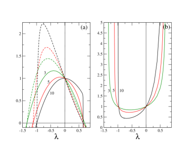
Figure 2: (Color on line) (a) Plots of $\det C^{l}_{w}(\lambda,t)/\det C$ (solid lines) and $\det(C^{r}_{w}(\lambda,t)+C)/\det C$ (dashed lines) versus $\lambda$ for $t=3,5,10$ and $\tau=1$. (b) Corresponding moment generating function $G_{w,\lambda}(t)$.

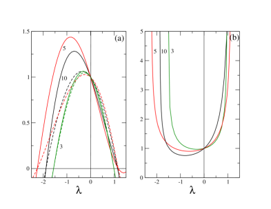
Figure 3: (Color on line) (a) Plots of $\det C^{l}_{w}(\lambda,t)/\det C$ (solid lines) and $\det(C^{r}_{\rm o}(\lambda,t)+C)/\det C$ (dashed lines) versus $\lambda$ for $t=3,5,10$ and $\tau=3$. (b) Corresponding moment generating function $G_{w,\lambda}(t)$.

Two typical examples of the evolution of the determinants with $\lambda$ at different times are shown in Figs. 2 and 3 together with the corresponding moment generating functions. The calculations are performed for the observable ${\cal W}_{t}$ but the same type of results are obtained for the other observables. Inspection of the characteristic polynomial $p_{H}(s)$ reveals that $\lambda_{\min}=-472.080$ and $\lambda_{\max}\simeq 1.019$ for $\tau=1$ and $\lambda_{\min}\simeq-5.118$ and $\lambda_{\max}\simeq 1.665$ for $\tau=3$. Moreover, it is found that $T_{x}/T\approx 1.663$, $T_{v}/T\approx 0.570$ for $\tau=1$ and $T_{x}/T\approx 1.152$, $T_{v}/T\approx 0.857$ for $\tau=3$. We can thus infer from Eq. (63) that the matrices $C^{r}_{w}(\lambda,t)+C$ and $C^{l}_{w}(\lambda,t)$ are always positive definite and the generating function $G_{w,\lambda}(t)$ is always finite for values of $\lambda$ in the range $0\leq\lambda\lesssim 0.601$ for $\tau=1$ and $0\leq\lambda\lesssim 0.868$ for $\tau=3$.

By comparing Figs. 2 and 3, we can see at once that the width of the interval ${\cal D}_{w}(t)$ does not decrease monotonically with time for $\tau=3$, in contrast to the case $\tau=1$. (Note in passing that $G_{w,\lambda}(t)$ does not satisfy the symmetry $\lambda\leftrightarrow 1-\lambda$; see the discussion in Ref. RTM2017 .) The difference between these two cases is even more manifest if we plot the evolution of the determinants with $t$ at fixed $\lambda$, as done in Fig. 4 (for brevity, we only show the behavior of $\det C^{l}_{w}(\lambda,t)$ and focus on negative values of $\lambda$).

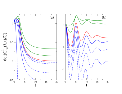
Figure 4: (Color on line) Time evolution of $\det C^{l}_{w}(\lambda,t)/\det C$ for $\tau=1$ (a) and $\tau=3$ (b). The values of $\lambda$ decrease from top to bottom and $\det C^{l}_{w}(\lambda,t)$ is always positive for $\lambda\gtrsim-0.963$ (red curve in panel a) or $\lambda\gtrsim-1.51$ (red curve in panel b). The parts of the curves corresponding to $\det C^{l}_{w}(\lambda,t)<0$ are plotted as dashed lines.

In both cases, there is a critical value of $\lambda$ above which $\det C^{l}_{w}(\lambda,t)>0$ at all times and the generating function is always finite. For smaller values of $\lambda$, Figs. 4(a) and 4(b) depict two different scenarios. For $\tau=1$, the determinant vanishes at a unique time $t^{-}_{w}(\lambda)$ which increases monotonically to infinity as $\lambda$ approaches the critical value. In this case $t^{-}_{w}(\lambda)$ is just the inverse function of $\lambda_{w}^{-}(t)$. For $\tau=3$, the curves cross the $t$ axis a number of times (as the smallest eigenvalue of the matrix changes its sign), so that the determinant is positive in a certain time range, then negative, then positive again, etc. The function $t^{-}_{w}(\lambda)$ is thus multivalued and the fact that the positive parts of the curves disappear at different times explains the non-monotonic behavior observed in Fig. 3 as $t$ varies.

A similar behavior is observed for $\lambda>0$ and this eventually leads to Figs. 5(a) and 5(b) which describe how the domain of existence of $G_{w,\lambda}(t)$ evolves with time. Note that $\lambda_{w}^{+}(t)>0.601$ for $\tau=1$ and $\lambda_{w}^{+}(t)>0.868$ for $\tau=3$, in agreement with the predictions of Eq. (63).

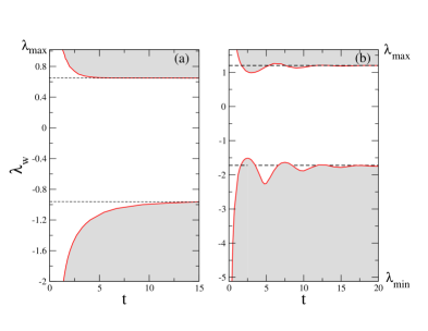
Figure 5: (Color on line) Evolution of the domain of existence of the generating function $G_{w,\lambda}(t)$, the interval ${\cal D}_{w}(t)=\big{(}\lambda^{+}_{w}(t),\lambda^{-}_{w}(t)\big{)}$, for $\tau=1$ (a) and $\tau=3$ (b). The matrices $C+C^{r}_{w}(\lambda,t)$ and $C_{w}^{l}(\lambda,t)$ are positive definite and $G_{w,\lambda}(t)$ is finite in the unshaded regions. At fixed $t$, $G_{w,\lambda}(t)$ diverges as $\lambda\to\lambda^{+}_{w}(t)$ and $\lambda\to\lambda^{-}_{w}(t)$ (solid red lines). The black dashed lines indicate the limits $\lambda_{w1}$ and $\lambda_{w2}$ of the interval $\hat{\cal D}_{w}$ (see Fig. 8 below).

We stress that the generating function $G_{w,\lambda}(t)$ is finite at time $t$ if $\det C_{w}^{l}(\lambda,t)>0$ whatever the sign of the determinant for $t^{\prime}<t$. Otherwise, one would not obtain the same values of the thresholds $\lambda_{w}^{-}(t)$ and $\lambda_{w}^{+}(t)$ by varying $\lambda$ at fixed $t$ or varying $t$ at fixed $\lambda$, and the results displayed in Fig. 4(b) would not be consistent with those in Fig. 3. We thus disagree with the statement made by C. Kwon et al in Ref. KNP2011 that the generating function is well defined only when the determinant is positive for all $t^{\prime}<t$, which implies that the threshold is “frozen” beyond a critical time. For $\tau=3$, this would amount to rejecting the non-monotonic dependence of $\lambda^{+}_{w}(t)$ and $\lambda^{-}_{w}(t)$ on time displayed in Fig. 5(b). We therefore dispute the claim that the generating function jumps discontinuously to infinity beyond this critical time (see Fig. 2(b) in Ref. KNP2011 ) and we challenge the existence of the so-called “dynamic phase transitions” discussed in Refs. KNP2011 ; NKP2013 ; KNP2013 .

In fact, the behavior of $\lambda_{w}^{-}(t)$ and $\lambda_{w}^{+}(t)$ with $t$ can be directly checked by looking at the pdf $P_{t}(\beta{\cal W}_{t}={\cal W})$. Indeed, the divergences of $G_{w,\lambda}(t)$ at $\lambda^{\pm}_{w}(t)$ signal that $P_{t}({\cal W})$ has exponential tails. More precisely, the numerical solution of the RDE (42a) reveals that $\det C_{w}^{l}(\lambda,t)\sim\det(C_{w}^{r}(\lambda,t)+C)\sim(\lambda-\lambda^{\pm}_{w}(t))$ as $\lambda\to\lambda^{\pm}_{w}(t)$, so that, from Eqs. (48),

$$G_{w,\lambda}(t)\sim(\lambda-\lambda^{\pm}_{w}(t))^{-1/2}$$ (104)

and, thus KNP2011 ,

$$P_{t}({\cal W})\sim\frac{e^{\lambda^{\mp}_{w}(t){\cal W}}}{\sqrt{|{\cal W}|}}\ ,\>\>{\cal W}\to\pm\infty\ .$$ (105)

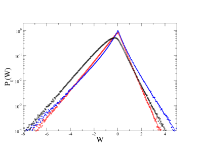
Figure 6: (Color on line) The pdf $P_{t}({\cal W})$ versus ${\cal W}$ for $\tau=3$ at different times: $t=3$ (blue stars), $5$ (red circles), and $10$ (black squares). $P_{t}({\cal W})$ is obtained from numerical simulations of $N=5.10^{6}$ samples. The straight lines on the right-hand side correspond to the asymptotic form (105) with the numerical values of $\lambda_{w}^{-}(t)$ taken from Fig. 5(b).

In Fig. 6, the pdf obtained by numerically integrating the set of dynamical equations (II.1) for $n=5$ and $\tau=3$ is plotted in the semi-log scale. It is manifest that the slopes of the tails of the pdf do not vary monotonically with time and they are very well described by the asymptotic form (105) (see the solid lines on the right-hand side).

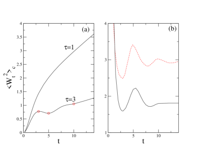
Figure 7: (Color on line) (a) Time evolution of the variance $\langle W_{t}^{2}\rangle_{c}$ for $\tau=1$ and $\tau=3$. The circles represent the results of the numerical simulation. (b) The width $l_{w}(t)=\lambda_{w}^{+}(t)-\lambda_{w}^{-}(t)$ of the interval ${\cal D}_{w}(t)$ for $\tau=3$ (red dashed line) is compared to $[\langle W_{t}^{2}\rangle_{c}-\mu_{w}^{\prime\prime}(0)t]^{-1}$ (solid black line).

Remarkably, the nontrivial behavior of $\lambda_{w}^{\pm}(t)$ for $\tau=3$ also affects the variance $\langle W^{2}_{t}\rangle_{c}=\langle W_{t}^{2}\rangle-\langle W_{t}\rangle^{2}=\partial^{2}\ln G_{w,\lambda}(t)/\partial^{2}\lambda|_{\lambda=0}$. As shown in Fig. 7, the non-monotonic variation of $\langle W^{2}_{t}\rangle_{c}$ for $\tau=3$ is related to the evolution of the width $l_{w}(t)=\lambda_{w}^{+}(t)-\lambda_{w}^{-}(t)$ of the interval ${\cal D}_{w}(t)$. Since the variance is larger when $l_{w}(t)$ is smaller and $\langle W_{t}^{2}\rangle_{c}\sim\mu_{w}^{\prime\prime}(0)t$ as $t\to\infty$ (where $\mu_{w}(\lambda)=f^{+}(\lambda)$ is the SCGF - see Sec. IV.2.3 below), this relation is made more visible by comparing $l_{w}(t)$ to the inverse of $\langle W_{t}^{2}\rangle_{c}-\mu_{w}^{\prime\prime}(0)t$, as done in Fig. 7(b). So the pdf $P_{t}({\cal W})$ does not necessarily become more distributed as $t$ increases, as could be naively expected.

IV.2 Long-time behavior

IV.2.1 Domain of existence of the scaled-cumulant generating function (SCGF)

We now focus on the behavior for $t\to\infty$. As can be seen in Fig. 5, the thresholds $\lambda_{w}^{\pm}(t)$ converge to finite values $\lambda_{w}^{\pm}(\infty)$. More generally, for an observable $\rm o$, ${\cal D}_{\rm o}(t)\to{\cal D}_{\rm o}(\infty)=\big{(}\lambda_{\rm o}^{-}(\infty),\lambda_{\rm o}^{+}(\infty)\big{)}$ with ${\cal D}_{\rm o}(\infty)\subseteq{\cal D}_{H}$. On the other hand, the analysis of Sec. III.2.2 tells us that $C^{r}_{\rm o}(\lambda,t)\to\hat{C}^{r,+}(\lambda)$ and $C^{l}_{\rm o}(\lambda,t)\to\hat{C}^{l,+}(\lambda)$ for generic values of $\lambda\in{\cal D}_{H}$ (i.e., for values of $\lambda$ such that $\det\hat{C}^{l,+}_{\rm o}(\lambda)\neq 0$ and $\det(\hat{C}^{r,+}_{\rm o}(\lambda)+C)\neq 0$). Therefore, ${\cal D}_{\rm o}(\infty)$, the domain of existence of the SCGF, coincides with the interval $\hat{\cal D}_{\rm o}=(\lambda_{\rm o1},\lambda_{\rm o2})$ for which the matrices $\hat{C}^{r,+}_{\rm o}(\lambda)+C$ and $\hat{C}^{l,+}_{\rm o}(\lambda)$ are both positive definite. Generically,

$${\cal D}_{\rm o}(\infty)=\hat{\cal D}_{\rm o}\subseteq{\cal D}_{H},$$ (106)

with $\hat{\cal D}_{\rm o}={\cal D}_{H}$ when these matrices $\hat{C}^{r,+}_{\rm o}(\lambda)+C$ and $\hat{C}^{l,+}_{\rm o}(\lambda)$ are positive definite for all $\lambda\in{\cal D}_{H}$.

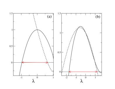
Figure 8: (Color on line) $\det\hat{C}^{l,+}_{w}(\lambda)/\det C$ (solid lines) and $\det(\hat{C}^{r,+}_{w}(\lambda)+C)/\det C$ (dashed lines) as a function of $\lambda$ for $\tau=1$ (a) and $\tau=3$ (b) (in both panels, the largest value of $\lambda$ is $\lambda_{\max}$). The arrows indicate the range $\hat{\cal D}_{w}$ of values of $\lambda$ for which the matrices $\hat{C}^{r,+}_{w}(\lambda)+C$ and $\hat{C}^{l,+}_{w}(\lambda)$ are both positive definite.

This is verified numerically in Fig. 8 which shows the variation of the determinants of $\hat{C}^{r,+}_{w}(\lambda)+C$ and $\hat{C}^{l,+}_{w}(\lambda)$ with $\lambda$ for the same values of the parameters as in Figs. 2-7. For $\tau=1$ and $\tau=3$, it is found that the two determinants are positive for $\lambda\in(-0.963,0.649)$ and $\lambda\in(-1.722,1.200)$, respectively, and these values are in excellent agreement with the thresholds $\lambda_{w}^{-}(\infty)$ and $\lambda_{w}^{+}(\infty)$ that can be extrapolated from Fig. 5. Note that $\lambda_{w1}$, the lower limit of the interval $\hat{\cal D}_{w}$, here corresponds to $\det\hat{C}^{l,+}_{w}(\lambda_{w1})=0$ (with $\det(\hat{C}^{r,+}_{w}(\lambda_{w1})+C)\neq 0$) whereas $\lambda_{w2}$, the upper limit, corresponds to $\det(\hat{C}^{r,+}_{w}(\lambda_{w2})+C)=0$ (with $\det\hat{C}^{l,+}_{w}(\lambda_{w2})\neq 0$).

At first sight, the latter observation may seem to contradict the fact that the determinants of the matrices $C^{l}_{w}(\lambda,t)$ and $C^{r}_{w}(\lambda,t)+C$ vanish for the same values of $\lambda$, i.e., $\lambda_{w}^{-}(t)$ or $\lambda_{w}^{+}(t)$ (see Figs. 2 and 3). To solve this puzzle we need to look more closely into the long-time behavior of the determinants at the boundaries of the interval $\hat{\cal D}_{w}=(\lambda_{w1},\lambda_{w2})$. This is done in Fig. 9 for $\tau=1$ where for conciseness we only consider the behavior of $\det(C^{r}_{w}(\lambda,t)+C)$ in the vicinity of $\lambda_{w1}\simeq-0.963$.

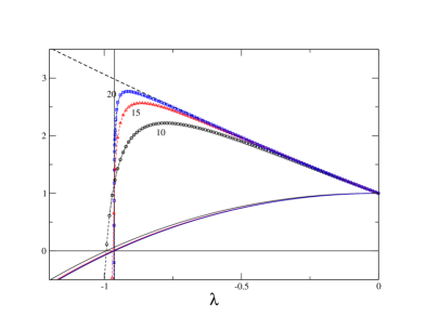
Figure 9: (Color on line) $\det(C^{r}_{w}(\lambda,t)+C)/\det C$ (symbols) and $\det(C^{l}_{w}(\lambda,t)/\det C$ (solid lines) as a function of $\lambda$ for $\tau=1$ and $t=10,15,20$. The solid and dashed black lines represent $\det\hat{C}_{w}^{l,+}(\lambda)/\det C$ and $\det(\hat{C}_{w}^{r,+}(\lambda)+C)/\det C$, respectively, like in Fig. 8.

Figure 10: (Color on line) Time evolution of $\det C_{w}^{l}(\lambda,t)/\det C$ (solid lines) and $\det(C^{r}_{w}(\lambda,t)+C)/\det C$ (dashed lines) for $\tau=1$ and different values of $\lambda$ close to $\lambda_{w1}\simeq-0.963$. The red lines correspond to $\lambda=\lambda_{w1}$.

What this figure reveals is that $\det(C^{r}_{w}(\lambda,t)+C)$ strongly deviates from $\det(\hat{C}^{r,+}_{w}(\lambda)+C)$ as $\lambda$ decreases before vanishing at $\lambda=\lambda_{w}^{-}(t)$. This contrasts with the behavior of $\det C^{l}_{w}(\lambda,t)$ that smoothly approaches $\det\hat{C}^{l,+}_{w}(\lambda)$ as $t$ increases. In addition, $\det(C^{r}_{w}(\lambda,t)+C)$ diverges to $-\infty$ for $\lambda$ very close to (but smaller than) $\lambda_{w}^{-}(t)$, signaling that the solution of the RDE (42a) blows up. Another striking feature is that the value of the determinant for $\lambda=\lambda_{w1}$ (indicated by the vertical line in the figure) is approximately independent of time (as the three representative curves cross each other at almost the same point). This suggests that $\lim_{t\to\infty}\det(C^{r}_{w}(\lambda_{w1},t)+C)$ is finite but differs from $\det(\hat{C}^{r,+}_{w}(\lambda_{w1})+C)$. This is indeed confirmed by Fig. 10 which shows the time evolution of $\det C_{w}^{l}(\lambda,t)$ and $\det(C^{r}_{w}(\lambda,t)+C)$ for values of $\lambda$ close to $\lambda_{w1}$. One can see that $\det(C^{r}_{w}(\lambda_{w1},t)+C)/\det C\approx 1.17$ at large times whereas $\det(\hat{C}^{r,+}_{w}(\lambda_{w1})+C)/\det C\approx 2.98$.

This phenomenon is rather subtle but should come as no surprise. Indeed, as predicted by Eq. (85a), the condition $\det C_{\rm o}^{l,+}(\lambda_{w1})=0$ implies that the solution of the RDE (42a) does not go asymptotically to $\hat{C}_{\rm o}^{r,+}(\lambda_{w1})$ and, as a result, $\det(C^{r}_{w}(\lambda_{w1},t\to\infty)+C)\neq\det(C^{r,+}_{w}(\lambda_{w1})+C)$. As a matter of fact, a similar behavior takes place in the vicinity of $\lambda_{w2}$, with the roles of $C^{r}_{w}(\lambda,t)+C$ and $C^{l}_{w}(\lambda,t)$ inverted, and it is also observed for $\tau=3$. More generally, this is one of the two scenarios that may occur at the limits of the domain of definition of the SCGF when $\hat{\cal D}_{\rm o}\subset{\cal D}_{H}$ (i.e., $\lambda_{\rm o1}>\lambda_{\min}$ and $\lambda_{\rm o2}<\lambda_{\max}$). This is a nontrivial issue which will be further discussed in Sec. IV.3. An important case is $\lambda_{\rm o2}=1$, as it concerns the fluctuation theorem (16) for the heat and the conjecture (17) for the apparent entropy production.

IV.2.2 Expressions of the SCGF and of the pre-exponential prefactors

Now that the domain of existence of the SCGF has been identified as $\hat{\cal D}_{\rm o}=(\lambda_{\rm o1},\lambda_{\rm o,2})$, we derive explicit expressions for the SCGF $\mu_{\rm o}(\lambda)$ and the pre-exponential factors $g_{\rm o}(\lambda)$ when $\lambda_{\rm o1}<\lambda<\lambda_{\rm o2}$. Since $C^{r}_{\rm o}(\lambda,t)+C\to\hat{C}^{r,+}_{\rm o}(\lambda)+C>0$ and $C^{l}_{\rm o}(\lambda,t)\to\hat{C}^{l,+}_{\rm o}(\lambda)>0$, we have

$$f^{r}_{\rm o}(\lambda,t)\to f^{+}(\lambda)$$

$$f^{l}_{\rm o}(\lambda,t)\to f^{+}(\lambda)\ ,$$ (107)

and from Eqs. (40) we obtain the two asymptotic expressions

$$G^{r}_{\rm o,\lambda}({\bf u}_{0},t)\sim g^{r}_{\rm o}(\lambda)\exp\big{(}-\frac{1}{2}{\bf u}_{0}^{T}\hat{C}^{r,+}_{\rm o}(\lambda){\bf u}_{0}\big{)}e^{f^{+}(\lambda)t}$$ (108a)

$$G^{l}_{\rm o,\lambda}({\bf u},t)\sim g^{l}_{\rm o}(\lambda)\exp\big{(}-\frac{1}{2}{\bf u}^{T}\hat{C}^{l,+}_{\rm o}(\lambda){\bf u}\big{)}e^{f^{+}(\lambda)t}\ ,$$ (108b)

with

$$g^{r}_{\rm o}(\lambda) =\exp\left(\int_{0}^{\infty}dt\>[f^{r}_{\rm o}(\lambda,t)-f^{+}(\lambda)]\right)$$ (109a)

$$g^{l}_{\rm o}(\lambda) =\left(\frac{\det C}{(2\pi)^{n+2}}\right)^{1/2}\exp\left(\int_{0}^{\infty}dt\>[f^{l}_{\rm o}(\lambda,t)-f^{+}(\lambda)]\right)\ .$$ (109b)

Integrating $G^{r}_{\rm o,\lambda}({\bf u}_{0},t)p({\bf u}_{0})$ over the initial state ${\bf u}_{0}$ and $G^{l}_{\rm o,\lambda}({\bf u},t)$ over the final state ${\bf u}$, we finally get

$$G_{\rm o,\lambda}(t)\sim g_{\rm o}(\lambda)e^{f^{+}(\lambda)t}\ ,$$ (110)

with

$$g_{\rm o}(\lambda) =\Big{[}\frac{\det[C+\hat{C}^{r,+}_{\rm o}(\lambda)]}{\det C}\Big{]}^{-1/2}\exp\left(\int_{0}^{\cal\infty}dt\>[f^{r}_{\rm o}(\lambda,t)-f^{+}(\lambda)]\right)$$ (111a)

$$=\Big{[}\frac{\det\hat{C}^{l,+}_{\rm o}(\lambda)}{\det C}\Big{]}^{-1/2}\exp\left(\int_{0}^{\cal\infty}dt\>[f^{l}_{\rm o}(\lambda,t)-f^{+}(\lambda)]\right)\ .$$ (111b)

Eq. (110) is a central result of our work as it shows that for $\lambda\in\hat{\cal D}_{\rm o}$ the SCGF $\mu_{\rm o}(\lambda)$ defined in Eq. (29) is equal to the function $f^{+}(\lambda)$ which is associated with the maximal solutions of the CAREs (86). The SCGF is therefore the same for the three observables ${\cal W}_{t},{\cal Q}_{t}$ and $\Sigma_{t}$ since the corresponding matrices $B_{\rm o}$ have the same anti-symmetric part, which implies that the Hamiltonian matrices have the same spectrum. On the other hand, the interval $\hat{\cal D}_{\rm o}$ and the pre-exponential factor $g_{\rm o}(\lambda)$ depend on the observable. In particular, the expressions (111) of $g_{\rm o}(\lambda)$ diverge at the boundaries of $\hat{\cal D}_{\rm o}$.

The SCGF can be computed from Eq. (99), i.e., from the eigenvalues of the Hamiltonian matrices. This is a standard numerical task, even for large $n$, but we now derive an equivalent and even more convenient expression as an integral over frequency. To this end, we use the property that each symmetric solution, $\hat{C}_{\rm o}^{r,(\alpha)}(\lambda)$ or $\hat{C}_{\rm o}^{l,(\alpha)}(\lambda)$, of the CAREs gives rise to a factorization of the characteristic polynomial $p_{H}(\lambda,s)$ of $H^{r}_{\rm o}(\lambda)$ and $H^{l}_{\rm o}(\lambda)$ in the form K2010

$$p_{H}(\lambda,s)=(-1)^{n}q^{(\alpha)}(\lambda,s)q^{(\alpha)}(\lambda,-s)\ ,$$ (112)

where $q^{(\alpha)}(\lambda,s)$ is the characteristic polynomial of the matrices $-A_{\rm o}(\lambda)+D\hat{C}_{\rm o}^{r,(\alpha)}(\lambda)$ and $A_{\rm o}(\lambda)+D\hat{C}_{\rm o}^{l,(\alpha)}(\lambda)$. (Owing to the invariance relations (91), $q^{(\alpha)}(\lambda,s)$ does not depend on the observable.) Eq. (112) follows from

$$\begin{bmatrix}I_{n+2}&0\\ \hat{C}^{r,(\alpha)}_{\rm o}(\lambda)&I_{n+2}&\end{bmatrix}^{-1}H^{r}_{\rm o}(\lambda)\begin{bmatrix}I_{n+2}&0\\ \hat{C}^{r,(\alpha)}_{\rm o}(\lambda)&I_{n+2}&\end{bmatrix}=\begin{bmatrix}-A_{\rm o}(\lambda)+D\hat{C}^{r,(\alpha)}_{\rm o}(\lambda)&D\\ 0&[A_{\rm o}(\lambda)-D\hat{C}^{r,(\alpha)}_{\rm o}(\lambda)]^{T}&\end{bmatrix}$$ (113)

and a similar relation involving $C^{l,(\alpha)}_{\rm o}(\lambda)$ and $H^{l}_{\rm o}(\lambda)$. Focusing on the maximal solutions $\hat{C}^{r,+}_{\rm o}(\lambda)$ and $\hat{C}^{l,+}_{\rm o}(\lambda)$, we then define the rational function

$$G^{+}(\lambda,s)=\frac{q^{+}(\lambda,s)}{p_{A}(s)}\ ,$$ (114)

where $p_{A}(s)$ is the characteristic polynomial of the drift matrix $A$ given by Eq. (24). As a result, $G^{+}(\lambda,s)$ has $n+2$ zeros but no poles in the closed right half plane (since all eigenvalues of $A$ have a negative real part). In addition,

$$q^{+}(\lambda,s)=\prod_{i=1}^{n+2}(s-s_{i}^{+})=s^{n+2}-(\sum_{i}^{n+2}s_{i}^{+})s^{n+1}+...$$ (115)

and

$$p_{A}(s)=s^{n+2}-\mbox{Tr}(A)s^{n+1}+...\ ,$$ (116)

so that the function $L^{+}(\lambda,s)$ defined through

$$G^{+}(\lambda,s)=[1+L^{+}(\lambda,s)]^{-1}$$ (117)

has a relative degree equal to $1$. (The relative degree is the difference between the degrees of the polynomials in the denominator and in the numerator. In control theory, $L^{+}_{\lambda}(s)$ would be interpreted as a proper, scalar rational loop transfer function of a feedback system B2021 ; AM2008 .) A standard application of Cauchy’s residue theorem, known as Bode’s sensitivity integral in control theory B2021 ; AM2008 , then yields

$$\frac{1}{2\pi i}\int_{-i\infty}^{i\infty}ds\>\ln|G^{+}(\lambda,s)|=\sum_{i=1}^{n+2}s_{i}^{+}(\lambda)-\frac{1}{2}\kappa^{+}(\lambda)\ ,$$ (118)

where the integration is performed along the imaginary axis in the complex $s$-plane, and

$$\kappa^{+}(\lambda) \equiv\lim_{s\to\infty}sL^{+}(\lambda,s)=\lim_{s\to\infty}s\frac{p_{A}(s)-q^{+}(\lambda,s)}{p_{A}(s)}$$

$$=\sum_{i=1}^{n+2}s_{i}^{+}(\lambda)-\mbox{Tr}(A)\ .$$ (119)

Inserting Eqs. (118) and (IV.2.2) into Eq. (99), we obtain that

$$f^{+}(\lambda)=-\frac{1}{2\pi i}\int_{-i\infty}^{i\infty}ds\>\ln|G^{+}(\lambda,s)|,$$

which thanks to Eqs. (112), (114), and (72) can then be rewritten as

$$f^{+}(\lambda) =-\frac{1}{4\pi i}\int_{-i\infty}^{i\infty}ds\>\ln\frac{(-1)^{n}p_{H}(\lambda,s)}{|p_{A}(s)|^{2}}$$

$$=-\frac{1}{4\pi i}\int_{-i\infty}^{i\infty}ds\>\ln\Big{[}1-\frac{2\lambda g}{Q_{0}^{2}}(\frac{n}{\tau})^{2n}s\frac{(1-\frac{s\tau}{n})^{n}-(1+\frac{s\tau}{n})^{n}}{|p_{A}(s)|^{2}}\Big{]}\ .$$ (121)

Note that the integral is finite as $p_{H}(\lambda,s)$ has no purely imaginary roots for $\lambda\in{\cal D}_{H}$.

We can further transform Eq. (IV.2.2) by replacing the Laplace variable $s$ by the frequency $\omega=is$ and introducing the response function $\chi_{n}(\omega)$ defined in Fourier space by $x(\omega)=\chi_{n}(\omega)\xi(\omega)$. It is readily found from Eq. (4) that

$$\chi_{n}(\omega)=\Big{(}-\omega^{2}-\frac{i\omega}{Q_{0}}+1-\frac{g}{Q_{0}}(1-\frac{i\omega\tau}{n})^{-n}\Big{)}^{-1}\ ,$$ (122)

which can be also expressed as

$$\chi_{n}(\omega) =(\frac{n}{\tau})^{n}\frac{(1-\frac{i\omega\tau}{n})^{n}}{p_{A}(s=-i\omega)}$$ (123)

by using Eq. (24). Eq. (IV.2.2) is then recast as

$$f^{+}(\lambda) =-\frac{1}{2}\int\frac{d\omega}{2\pi}\>\ln\Big{[}1-\frac{4\lambda g}{Q_{0}^{2}}\omega\sin_{n}(\omega\tau)|\chi_{n}(\omega)|^{2}\Big{]}\ ,$$ (124)

where we have defined the $n$-dependent sine-like function

$$\sin_{n}(x)=\frac{1}{2i}[(1-\frac{ix}{n})^{-n}-(1+\frac{ix}{n})^{-n})]$$ (125)

which satisfies $\lim_{n\to\infty}\sin_{n}(x)=\sin(x)$. As a consequence, $f^{+}(\lambda)$ is simply expressed in terms of the spectral density $|\chi_{n}(\omega)|^{2}$. This shows the connection between the Riccati formalism and the results in the mathematical literature BD1997 ; BGR1997 ; GRZ1999 ; ZS2023 for the SCGF of stationary Gaussian processes.

Figure 11: (Color on line) (a) Function $f^{+}(\lambda)$ computed from Eq. (124) for $n=5$, $\tau=1$ and $\tau=3$. The parts of the curves in red correspond to the interval $\hat{\cal D}_{w}$ for which the SCGF $\mu_{w}(\lambda)$ is finite and equal to $f^{+}(\lambda)$ (see Fig. 8) and the vertical dashed lines indicate the limits $\lambda_{\min}$ and $\lambda_{\max}$ of ${\cal D}_{H}$, the interval of definition of $f^{+}(\lambda)$ ($\lambda_{\min}\approx-472.8$ for $\tau=1$, which is outside the scale of the figure). (b) Corresponding rate function $I_{w}(a)$. The parts of the curves in red are obtained from the Legendre transform (126) and the linear parts in black are obtained from Eqs. (127).

The behavior of $f^{+}(\lambda)$ with $\lambda$ for $n=5$, $\tau=1$ and $\tau=3$ is shown in Fig. 11(a). This illustrates two important properties of the function: i) $f^{+}(\lambda)$ has infinite slopes at the boundaries of ${\cal D}_{H}$ and ii) $f^{+}(\lambda)$ is convex in ${\cal D}_{H}$ (we already know that this function is differentiable). Accordingly, the Legendre-Fenchel transform (31) that relates the SCGF to the rate function reduces to the usual Legendre transform. Specifically, defining $\lambda^{*}(a)$ as the (unique) solution of $df^{+}(\lambda)/d\lambda|_{\lambda=\lambda^{*}}=-a$, one has T2009

$$I(a)=-a\lambda^{*}-f^{+}(\lambda^{*})\>\>\>\mbox{for}\>\>\lambda^{*}(a)\in\hat{\cal D}_{\rm o}\ .$$ (126)

If $\hat{\cal D}_{\rm o}={\cal D}_{H}$ the function $I(a)$, which does not depend on the observable, is asymptotically linear as $a\to-\infty$ (resp. $a\to+\infty$) with slope $-\lambda_{\max}$ (resp. $-\lambda_{\min}$). This means that the values of $\lambda$ outside ${\cal D}_{H}$ are irrelevant to the determination of the rate function, which justifies our initial choice to restrict the study of the solutions of the Riccati equations to this interval.

On the other hand, if $\hat{\cal D}_{\rm o}\subset{\cal D}_{H}$ (where here and below $\subset$ means a strict inclusion), the condition $\lambda^{*}(a)\in\hat{\cal D}_{\rm o}$ defines two special values $a_{\rm o}^{-}=-df^{+}(\lambda)/d\lambda|_{\lambda_{\rm o2}}$ and $a_{\rm o}^{+}=-df^{+}(\lambda)/d\lambda|_{\lambda_{\rm o1}}$ beyond which the rate function is no longer given by Eq. (126). Since $f^{+}(\lambda)$ has finite slopes at the two cutoff $\lambda_{\rm o1}$ and $\lambda_{\rm o2}$, the properties of Legendre transforms T2009 imply that the rate function (which now depends on the observable) exhibits linear branches beyond $a_{\rm o}^{\pm}$,

$$I_{\rm o}(a) =-a\lambda_{\rm o2}-f^{+}(\lambda_{\rm o2})\>\>\>\>\>a\leq a_{\rm o}^{-}$$ (127a)

$$I_{\rm o}(a) =-a\lambda_{\rm o1}-f^{+}(\lambda_{\rm o1})\>\>\>\>\>a\geq a_{\rm o}^{+}\ .$$ (127b)

This yields the curves $I_{w}(a)$ plotted in Fig. 11(b).

Finally, we consider the limit $n\to\infty$. It can be directly taken in Eq. (IV.2.2), replacing $(1\pm s\tau/n)^{n}$ by $e^{\pm s\tau}$ and using Eq. (25). This yields

$$\lim_{n\to\infty}\frac{(-1)^{n}p_{H}(\lambda,s)}{p_{A}(s)p_{A}(-s)}=1-\frac{2\lambda g}{Q_{0}^{2}}\frac{s(e^{-s\tau}-e^{s\tau})}{(s^{2}+\frac{s}{Q_{0}}+1-\frac{g}{Q_{0}}e^{-s\tau})(s^{2}-\frac{s}{Q_{0}}+1-\frac{g}{Q_{0}}e^{s\tau})}\ .$$ (128)

Alternatively, from Eq. (124),

$$f^{+}_{\infty}(\lambda)\equiv\lim_{n\to\infty}f^{+}(\lambda) =-\frac{1}{2}\int\frac{d\omega}{2\pi}\>\ln\Big{[}1-\frac{4\lambda g}{Q_{0}^{2}}\omega\sin(\omega\tau)|\chi_{\infty}(\omega)|^{2}\Big{]}\ ,$$ (129)

with

$$\chi_{\infty}(\omega)=(-\omega^{2}-\frac{i\omega}{Q_{0}}+1-\frac{g}{Q_{0}}e^{i\omega\tau})^{-1}\ .$$ (130)

As expected, this result coincides with the expression of the SCGF for the discrete delay obtained in our previous work RTM2017 by imposing periodic boundary conditions on the solution of the Langevin equation (i.e., $x(0)=x(t))$ and expanding $x(t)$ in a Fourier series (this amounts to assuming that boundary conditions can be neglected to leading order in $t$ in the calculation of $\langle e^{-\lambda{\cal A}_{t}}\rangle$; see, e.g., Ref. ZBCK2005 for a similar calculation). It is clear that Eq. (124) can be also derived by using the same method for $n$ finite.

IV.2.3 Relation with the spectral problem for the tilted generators

As is well known, the SCGF of additive functionals such as the ones considered in this work is given (in its domain of definition) by the dominant eigenvalue $\mu_{\rm o}(\lambda)$ of the tilted generators ${\cal L}_{\rm o,\lambda}$ and ${\cal L}^{\dagger}_{\rm o,\lambda}$ T2009 ; J2020 ; CT2015 ; T2018 . This results from the expansion of the restricted generating function $G_{\rm o,\lambda}({\bf u},t|{\bf u}_{0})$ in a complete basis of bi-orthogonal eigenfunctions, which yields asymptotically CT2015

$$G_{\rm o,\lambda}({\bf u},t|{\bf u}_{0})\sim r_{\rm o,\lambda}({\bf u}_{0})l_{\rm o,\lambda}({\bf u})e^{\mu_{\rm o}(\lambda)t}\ ,$$ (131)

where $r_{\rm o,\lambda}({\bf u}_{0})$ and $l_{\rm o,\lambda}({\bf u})$ are the right and left eigenfunctions associated with $\mu_{\rm o}(\lambda)$. Finding the SCGF thus requires solving the spectral problem

$${\cal L}_{\rm o,\lambda}\,r_{\rm o,\lambda}({\bf u}_{0}) =\mu_{\rm o}(\lambda)\,r_{\rm o,\lambda}({\bf u}_{0})$$ (132a)

$${\cal L}_{\rm o,\lambda}^{{\dagger}}\,l_{\rm o,\lambda}({\bf u}) =\mu_{\rm o}(\lambda)\,l_{\rm o,\lambda}({\bf u})\ ,$$ (132b)

with the eigenfunctions commonly normalized according to CT2015

$$\int d{\bf u}\>l_{\rm o,\lambda}({\bf u})r_{\rm o,\lambda}({\bf u})=1$$ (133a)

$$\int d{\bf u}\>l_{\rm o,\lambda}({\bf u})=1\ .$$ (133b)

(In particular, Eq. (133a) is inherited from the duality between the operators ${\cal L}_{\rm o,\lambda}$ and ${\cal L}^{\dagger}_{\rm o,\lambda}$ which imposes the boundary condition $l_{\rm o,\lambda}({\bf u})r_{\rm o,\lambda}({\bf u})=0$ at infinity T2018 .) Since we have shown above that the SCGF $\mu_{\rm o}(\lambda)$ is equal to $f^{+}(\lambda)$ inside its domain of definition $\hat{\cal D}_{\rm o}$, we already know the solution of the spectral problem for the dominant eigenvalue, and the eigenfunctions corresponding to $f^{+}(\lambda)$ are readily obtained from the asymptotic expressions (108) as

$$r_{\rm o,\lambda}({\bf u}_{0}) =g_{\rm o}^{r}(\lambda)\exp\left(-\frac{1}{2}{\bf u}_{0}^{T}\hat{C}^{r,+}_{\rm o}(\lambda){\bf u}_{0}\right)$$ (134a)

$$l_{\rm o,\lambda}({\bf u}) =\frac{g_{\rm o}^{l}(\lambda)}{\int d{\bf u}_{0}\>p({\bf u}_{0})r_{\rm o,\lambda}({\bf u}_{0})}\exp\left(-\frac{1}{2}{\bf u}^{T}\hat{C}^{l,+}_{\rm o}(\lambda){\bf u}\right)\ ,$$ (134b)

with $g_{\rm o}^{r}(\lambda)$ and $g_{\rm o}^{l}(\lambda)$ given by Eqs. (109). These expressions can be used to derive a simple expression of the prefactor $g_{\rm o}(\lambda)$. Inserting Eqs. (134) into Eq. (133a) and performing a few manipulations, we obtain the two relations

$$\exp\left(\int_{0}^{\cal\infty}dt\>[f^{r}_{\rm o}(\lambda,t)-f^{+}(\lambda)]\right)=\Big{[}\frac{\det[\hat{C}^{r,+}_{\rm o}(\lambda)+\hat{C}^{l,+}_{\rm o}(\lambda)]}{\det\hat{C}^{l,+}_{\rm o}(\lambda)}\Big{]}^{1/2}$$ (135a)

$$\exp\left(\int_{0}^{\cal\infty}dt\>[f^{l}_{\rm o}(\lambda,t)-f^{+}(\lambda)]\right)=\Big{[}\frac{\det[\hat{C}^{r,+}_{\rm o}(\lambda)+\hat{C}^{l,+}_{\rm o}(\lambda)]}{\det[C+\hat{C}^{r,+}_{\rm o}(\lambda)]}\Big{]}^{1/2}\ ,$$ (135b)

and using Eqs. (111) we find

$$g_{\rm o}(\lambda)=\left(\frac{\det C\>\det[\hat{C}^{l,+}_{\rm o}(\lambda)+\hat{C}^{r,+}_{\rm o}(\lambda)]}{\det\hat{C}^{l,+}_{\rm o}(\lambda)\>\det[\hat{C}^{r,+}_{\rm o}(\lambda)+C]}\right)^{1/2}\ .$$ (136)

This latter expression is another significant result of this work. It has the great advantage of no longer involving an integration over time; it suffices to compute the maximal solutions of the CAREs (86) from Eq. (88), which is a simple task.

Finally, after using Eqs. (135) and the normalization integral (133b), the expressions of $r_{\rm o,\lambda}({\bf u}_{0})$ and $l_{\rm o,\lambda}({\bf u})$ can be rewritten as

$$r_{\rm o,\lambda}({\bf u}_{0}) =\Big{[}\frac{\det[\hat{C}^{r,+}_{\rm o}(\lambda)+\hat{C}^{l,+}_{\rm o}(\lambda)]}{\det\hat{C}^{l,+}_{\rm o}(\lambda)}\Big{]}^{1/2}\exp\left(-\frac{1}{2}{\bf u}_{0}^{T}\hat{C}^{r,+}_{\rm o}(\lambda){\bf u}_{0}\right)$$ (137a)

$$l_{\rm o,\lambda}({\bf u}) =\Big{[}\frac{\det\hat{C}^{l,+}_{\rm o}(\lambda)}{(2\pi)^{n+2}}\Big{]}^{1/2}\exp\left(-\frac{1}{2}{\bf u}^{T}\hat{C}^{l,+}_{\rm o}(\lambda){\bf u}\right)\ .$$ (137b)

One can notice the similarity of these equations with Eqs. (55) and (56) in Ref. KSD2011 . In this paper, the large-time expression of the generating function for the heat flow in harmonic chains was computed by using finite-time Fourier transforms. As already mentioned, the expression (124) of the SCGF is easily obtained by this method. With more efforts, one can also compute the eigenfunctions, i.e., the matrices $\hat{C}^{r,+}_{\rm o}(\lambda)$ and $\hat{C}^{l,+}_{\rm o}(\lambda)$, and in turn the pre-exponential factors $g_{\rm o}(\lambda)$ (Eq. (136) is similar to Eq. (59) in Ref. KSD2011 ). However, this method has a major drawback which makes it impracticable for multidimensional systems: Each component of the matrices is given by an integral over frequency, so that the numerical computation becomes more and more burdensome as the dimensionality increases. Furthermore, one does not have access to the finite-time behavior of the generating functions and one cannot study the special cases where the solutions of the RDEs do not converge to $\hat{C}^{r,+}_{\rm o}(\lambda)$ and $\hat{C}^{l,+}_{\rm o}(\lambda)$ (see Sec. V). For all these reasons, the Riccati approach is much more illuminating and numerically effective.

IV.2.4 Effective process

From the knowledge of the eigenfunction $r_{\rm o,\lambda}({\bf u})$, one can build the so-called effective or driven process that describes how fluctuations of the observables are created dynamically in the long-time limit CT2015 . By construction, a given fluctuation $a$ of the time-intensive observable ${\cal A}_{t}/t$ in the original process is realized as a typical value in the effective process.

Since $r_{\rm o,\lambda}({\bf u})$ is a multivariate Gaussian, this process is again a linear diffusion,

$$\dot{{\bf u}}_{t}=\hat{A}(\lambda){\bf u}_{t}+{\boldsymbol{\xi}}_{t}\,,$$ (138)

with the same diffusion matrix $D$ as the original process but with a modified drift $\hat{\bf F}_{\lambda}=\hat{A}(\lambda){\bf u}$ given by CT2015

$$\hat{\bf F}_{\lambda} ={\bf F}+D(\nabla\ln r_{\rm o,\lambda}-\lambda{\bf g}_{\rm o})$$

$$=[A-D(\hat{C}^{r,+}_{\rm o}(\lambda)+\lambda B_{\rm o})]{\bf u}\ .$$ (139)

Hence, from the definition of the matrix $A_{\rm o}(\lambda)$ [Eq. (45)],

$$\hat{A}(\lambda)=A_{\rm o}(\lambda)-D\hat{C}^{r,+}_{\rm o}(\lambda).$$ (140)

By definition of the maximal solution $\hat{C}^{r,+}_{\rm o}(\lambda)$, the eigenvalues of $-\hat{A}(\lambda)$ belong to the subset ${\cal S}_{\lambda}^{+}$ of eigenvalues of the Hamiltonian matrices [see Eq. (87)] and therefore $-\hat{A}(\lambda)>0$. In addition, owing to Eqs. (91a) and (92a), $\hat{A}(\lambda)$ only depends on the antisymmetric part of the matrix $B_{\rm o}$. As a result, the driven process is the same for all observables having the same antisymmetric part (but it is only defined for $\lambda\in\hat{\cal D}_{\rm o}$, the domain of definition of the SCGF, which depends on the observable).

The corresponding invariant density is then given by CT2015

$$\hat{p}_{\lambda}({\bf u}) =r_{\rm o,\lambda}({\bf u})l_{\rm o,\lambda}({\bf u})=\big{[}(2\pi)^{n+2}\det\hat{\Sigma}(\lambda)\big{]}^{-1/2}\exp\left(-\frac{1}{2}{\bf u}^{T}\hat{\Sigma}^{-1}(\lambda){\bf u}\right)\ ,$$ (141)

with

$$\hat{\Sigma}(\lambda)=[\hat{C}^{r,+}_{\rm o}(\lambda)+\hat{C}^{l,+}_{\rm o}(\lambda)]^{-1}\ .$$ (142)

Using the fact that $\hat{C}^{r,+}_{\rm o}(\lambda)$ and $\hat{C}^{l,+}_{\rm o}(\lambda)$ are solutions of the CAREs (86a) and (86b), respectively, one can easily verify that $\hat{A}(\lambda)$ and $\hat{\Sigma}(\lambda)$ are related via the Lyapunov equation

$$\hat{A}(\lambda)\hat{\Sigma}(\lambda)+\hat{\Sigma}(\lambda)\hat{A}^{T}(\lambda)=-D\ ,$$ (143)

as it must be. We recall that the sum $\hat{C}^{r,+}_{\rm o}(\lambda)+\hat{C}^{l,+}_{\rm o}(\lambda)$ does not depend on the observable due to Eq. (90) and is positive definite, which guarantees that the invariant density exists and the driven process is ergodic.

The above equations are quite general and apply to any multidimensional linear diffusions but they take a simpler form for the model under study owing to the fact that $D_{ij}=\delta_{i1}\delta_{j1}$. The elements of the matrix $\hat{A}(\lambda)$ are then given by

$$\hat{A}_{ij}(\lambda)=[A_{\rm o}(\lambda)]_{ij}-[\hat{C}^{r,+}_{\rm o}(\lambda)]_{1j}\delta_{i1}.$$ (144)

Moreover, since $\hat{A}(\lambda)$ does not depend on the observable, we can choose $\rm o=w$, which yields

$$\hat{A}_{ij}(\lambda)=A_{ij}-[\hat{C}^{r,+}_{w}(\lambda)]_{1j}\delta_{i1}\ .$$ (145)

Therefore, only the first equation of the set of equations (II.1) is modified and replaced by

$$\dot{v}(t) =-\big{(}\frac{1}{Q_{0}}+[\hat{C}_{w}^{r,+}(\lambda)]_{11}\big{)}v(t)-x(t)+\frac{g}{Q_{0}}x_{n}(t)-\sum_{j=0}^{n}\>[\hat{C}_{w}^{r,+}(\lambda)]_{1(j+2)}\>x_{j}(t)+\xi(t)$$

$$=-\big{[}\frac{1}{Q_{0}}-2f^{+}(\lambda)\big{]}v(t)-\big{[}1+2f^{+}(\lambda)(f^{+}(\lambda)-\frac{1}{Q_{0}})\big{]}x(t)+\frac{g}{Q_{0}}x_{n}(t)-\sum_{j=1}^{n}\>[\hat{C}_{w}^{r,+}(\lambda)]_{1(j+2)}\>x_{j}(t)+\xi(t)\ ,$$ (146)

where we have used that $[\hat{C}_{w}^{r,+}(\lambda)]_{11}=-2f^{+}(\lambda)$ [Eq. (94a)] and $[\hat{C}_{w}^{r,+}(\lambda)]_{12}=2f^{+}(\lambda)(f^{+}(\lambda)-1/Q_{0})$ to derive the second line. After inserting the definition of the auxiliary variables $x_{j}(t)$ [Eq. (8)], the equation is finally recast as

$$\dot{v}(t)=-\big{[}\frac{1}{Q_{0}}-2f^{+}(\lambda)\big{]}v(t)-\big{[}1+2f^{+}(\lambda)(f^{+}(\lambda)-\frac{1}{Q_{0}})\big{]}x(t)+\int_{-\infty}^{t}ds\>[\frac{g}{Q_{0}}\>g_{n}(t-s,n/\tau)-h_{n}(\lambda,t-s)]x(s)+\xi(t)\ ,$$ (147)

where

$$h_{n}(\lambda,t)=\sum_{j=1}^{n}\>[\hat{C}_{w}^{r,+}]_{1(j+2)}\>g_{j}(t,n/\tau)\ .$$ (148)

Eq. (147) is another major result of this work. To our knowledge, this is the first explicit example of an effective process for a non-Markovian Langevin dynamics. Comparing with the original process governed by Eq. (4), we see that atypical fluctuations of the observable are created in the long-time limit by modifying not only the friction and the spring constants but also the memory kernel.

The stationary density associated with Eq. (147) is obtained by tracing out the auxiliary variables $u_{j}$ ($j\geq 2$) in Eq. (141), which leads to the bivariate Gaussian distribution

$$\hat{p}_{\lambda}(x,v)=\frac{1}{\pi Q_{0}\sqrt{\frac{\hat{T}_{x}(\lambda)}{T}\frac{\hat{T}_{v}(\lambda)}{T}}}e^{-\frac{1}{Q_{0}}(\frac{T}{\hat{T}_{x}(\lambda)}x^{2}+\frac{T}{\hat{T}_{v}(\lambda)}v^{2})}$$ (149)

characterized by the two $\lambda$-dependent temperatures $\hat{T}_{x}(\lambda)=(2T/Q_{0})\langle x^{2}\rangle_{\lambda}=(2T/Q_{0})\hat{\Sigma}_{22}(\lambda)$ and $\hat{T}_{v}(\lambda)=(2T/Q_{0})\langle v^{2}\rangle_{\lambda}=(2T/Q_{0})\hat{\Sigma}_{11}(\lambda)$ (here $\langle...\rangle_{\lambda}$ denotes an average over stochastic trajectories generated by the effective process in the stationary limit). Interestingly, the variances $\langle x^{2}\rangle_{\lambda}$ and $\langle v^{2}\rangle_{\lambda}$, and more generally all elements of the covariance matrix $\hat{\Sigma}(\lambda)$, can be expressed in terms of the spectral density $|\chi_{n}(\omega)|^{2}$, as the SCGF $f^{+}(\lambda)$.

To show this, we write the solution of the Lyapunov equation (143) as an integral over frequency of the spectrum matrix. Since $D_{ij}=\delta_{i1}\delta_{j1}$, we have G2004

$$\hat{\Sigma}_{ij}(\lambda)=\int\frac{d\omega}{2\pi}\langle{\bf u}(\omega){\bf u}^{T}(-\omega)\rangle_{\lambda}=\int\frac{d\omega}{2\pi}\hat{R}_{i1}(\lambda,\omega)\hat{R}_{j1}(\lambda,-\omega)\ ,$$ (150)

where $\hat{R}(\lambda,t)=e^{\hat{A}(\lambda)t}$ ($t>0$) is the response or Green’s function which reads in the Fourier space

$$\hat{R}(\lambda,\omega)=\int_{0}^{\infty}e^{\hat{A}(\lambda)t}e^{i\omega t}dt=-[\hat{A}(\lambda)+i\omega I_{n+2}]^{-1}\ .$$ (151)

Thanks to Eq. (145), the first column of $\hat{R}(\lambda,\omega)$ does not depend on $[\hat{C}^{r,+}_{\rm o}(\lambda)]_{1j}$ ($j=1,...,n+2)$, and from the expression of the drift matrix $A$ [Eq. (9)] we find

$$\hat{R}_{11}(\lambda,\omega)=\frac{i\omega(i\omega-\frac{n}{\tau})^{n}}{q^{+}(\lambda,s=i\omega)}$$ (152)

and

$$\hat{R}_{i1}(\lambda,\omega)=\frac{(-1)^{i-1}(\frac{n}{\tau})^{i-2}(i\omega-\frac{n}{\tau})^{n+2-i}}{q^{+}(\lambda,s=i\omega)}\ ,\>\>\>i=2,3,...,n+2\ ,$$ (153)

where $q^{+}(\lambda,s)=\prod_{i=1}^{n+2}[s-s_{i}^{+}(\lambda)]$ [Eq. (115)]. Inserting the above expressions into Eq. (150) and using Eqs. (72), (122), (123) and (125), we then obtain

$$\frac{\hat{T}_{x}(\lambda)}{T}=\frac{2}{Q_{0}}\hat{\Sigma}_{22}(\lambda) =\frac{2}{Q_{0}}\int\frac{d\omega}{2\pi}\frac{(\omega^{2}+\frac{n^{2}}{\tau^{2}})^{n}}{(-1)^{n}p_{H,\lambda}(s=i\omega)}$$

$$=\frac{2}{Q_{0}}\int\frac{d\omega}{2\pi}\frac{1}{|\chi_{n}(\omega)|^{-2}-\frac{4\lambda g}{Q_{0}^{2}}\omega\sin_{n}(\omega\tau)}$$ (154a)

$$\frac{\hat{T}_{v}(\lambda)}{T}=\frac{2}{Q_{0}}\hat{\Sigma}_{11}(\lambda) =\frac{2}{Q_{0}}\int\frac{d\omega}{2\pi}\frac{\omega^{2}(\omega^{2}+\frac{n^{2}}{\tau^{2}})^{n}}{(-1)^{n}p_{H,\lambda}(s=i\omega)}$$

$$=\frac{2}{Q_{0}}\int\frac{d\omega}{2\pi}\frac{\omega^{2}}{|\chi_{n}(\omega)|^{-2}-\frac{4\lambda g}{Q_{0}^{2}}\omega\sin_{n}(\omega\tau)}\ .$$ (154b)

Likewise,

$$\hat{\Sigma}_{n+2,1}(\lambda)=\langle x_{n}(t)v(t)\rangle_{\lambda} =\int\frac{d\omega}{2\pi}\frac{(\frac{n}{\tau})^{n}i\omega(i\omega+\frac{n}{\tau})^{n}}{(-1)^{n}p_{H}(\lambda,s=i\omega)}$$

$$=-\int\frac{d\omega}{2\pi}\frac{\omega\sin_{n}(\omega\tau)}{|\chi_{n}(\omega)|^{-2}-\frac{4\lambda g}{Q_{0}^{2}}\omega\sin_{n}(\omega\tau)}\ ,$$ (155)

and by comparing with the expression of $f^{+}(\lambda)$ [Eq. (124)], we find that $(2g/Q_{0}^{2})\langle x_{n}(t)v(t)\rangle_{\lambda}=-df^{+}(\lambda)/d\lambda$. This equality was expected. It expresses that if one is interested by a particular fluctuation in which the time-intensive observable $(2g/Q_{0}^{2})(1/t)\int_{0}^{t}dt^{\prime}x_{n}(t^{\prime})\circ dx(t^{\prime})$ takes the value $a$, this fluctuation is realized in the long-time limit as a typical value in the effective process, with $\lambda$ given by $a=-df^{+}(\lambda)/d\lambda$. (However, while the three observables ${\cal W}_{t}/t$, ${\cal Q}_{t}/t$ and $\Sigma_{t}/t$ are identical in the long-time limit, one must not forget that the Legendre duality only holds for $\lambda$ in the interval ${\hat{D}}_{\rm o}$ which depends on the observable.)

Figure 12: (Color on line) The function $h_{n}(\lambda,t)$ for $\lambda=0.5$, $\tau=1$ (a), $\tau=3$ (b), and increasing values of $n$: $n=5$ (green) $10,20,30,40,50$ (red).

Finally, we consider the limit $n\to\infty$. As illustrated in Fig. 12, the function $h_{n}(\lambda,t)$ appears to converge to a well-defined limit $h_{\infty}(\lambda,t)$. (We remind the reader that the SCGF $f^{+}(\lambda)$ and the matrix $\hat{C}_{\rm o}^{r,+}(\lambda)$ depend on $n$.) We thus expect the driven process for the discrete delay to be governed by the equation

$$\dot{v}(t) =-\big{[}\frac{1}{Q_{0}}-2f^{+}_{\infty}(\lambda)\big{]}v(t)-\big{[}1+2f^{+}_{\infty}(\lambda)(f^{+}_{\infty}(\lambda)-\frac{1}{Q_{0}})\big{]}x(t)+\frac{g}{Q_{0}}x(t-\tau)-\int_{-\infty}^{t}ds\>h_{\infty}(\lambda,t-s)x(s)+\xi(t)\ ,$$ (156)

where $f^{+}_{\infty}(\lambda)$ is given by Eq. (129) (see also Eq. (53) in Ref. RTM2017 ). The memory kernel does not reduce to a delta function in this limit. This interesting issue deserves a more complete study that we leave to future work.

Furthermore, we obtain from Eqs. (154)

$$\frac{\hat{T}_{x}(\lambda)}{T}\to\frac{2}{Q_{0}}\int\frac{d\omega}{2\pi}\frac{1}{|\chi_{\infty}(\omega)|^{-2}-\frac{4\lambda g}{Q_{0}^{2}}\omega\sin(\omega\tau)}$$ (157a)

$$\frac{\hat{T}_{v}(\lambda)}{T}\to\frac{2}{Q_{0}}\int\frac{d\omega}{2\pi}\frac{\omega^{2}}{|\chi_{\infty}(\omega)|^{-2}-\frac{4\lambda g}{Q_{0}^{2}}\omega\sin(\omega\tau)}\ ,$$ (157b)

with $\chi_{\infty}(\omega)$ given by Eq. (130).

IV.2.5 Role of (temporal) boundary terms

As we have seen in the previous sections, the average over the initial and final points of the stochastic trajectories may induce finite-time divergences in the moment generating functions and a reduction of the domain of existence of the SCGF from ${\cal D}_{H}$ to $\hat{\cal D}_{\rm o}$, which in turn induces linear branches in the rate function $I_{\rm o}(a)$.

It is natural to put this in relation to the role of the so-called “boundary” terms in the dynamical observables, i.e., terms that are not extensive in time such as $\Delta E$, the change in the internal energy of the system, which differentiates the heat from the work. This issue is well documented in the literature, both theoretically VC2003 ; Fa2002 ; V2006 ; BJMS2006 ; PRV2006 ; HRS2006 ; TC2007 ; Sab2011 ; N2012 ; NP2012 and experimentally (see Ref. C2017 and references therein). In particular, the breakdown of the Gallavotti-Cohen fluctuation relation GC1995 ; K1998 ; LS1999 can be attributed to such boundary terms which become relevant in the case of an unbounded potential. Things are more complicated in the presence of a continuous (non-Markovian) feedback, but fluctuations of work, heat, and entropy production are indeed different, as discussed in our previous work RTM2017 .

However, at odds with the assumption made in Ref. RTM2017 , the present numerical calculations show that $\hat{\cal D}_{w}\subset{\cal D}_{H}$ and the rate function $I_{w}(a)$ has linear branches (see Fig. 11) even though the stochastic work defined by Eq. (11) does not contain an explicit boundary term. This may come as a surprise, and one may argue that the definition (11) is misleading and that a boundary term does exist by decomposing $\beta{\cal W}_{t}=\int_{0}^{t}(B_{w}{\bf u}_{t^{\prime}})\circ d{\bf u}_{t^{\prime}}$ as

$$\beta{\cal W}_{t}=\frac{g}{Q_{0}^{2}}[x_{n}(t)x(t)-x_{n}(0)x(0)]+\frac{g}{Q_{0}^{2}}\int_{0}^{t}[x_{n}(t^{\prime})\circ dx(t^{\prime})-x(t^{\prime})\circ dx_{n}(t^{\prime})]\ .$$ (158)

This amounts to splitting the matrix $B_{w}$ defined by Eq. (21) into its symmetric and antisymmetric components, i.e.,

$$B_{w}=B_{w,sym}+B_{w,antisym}=\frac{g}{Q_{0}^{2}}\left(\begin{bmatrix}0&0&0&...&0\\ 0&0&0&...&1\\ 0&0&0&...&0\\ \vdots&\vdots&\vdots&\vdots&\vdots\\ 0&1&0&...&0&\end{bmatrix}+\begin{bmatrix}0&0&0&...&0\\ 0&0&0&...&1\\ 0&0&0&...&0\\ \vdots&\vdots&\vdots&\vdots&\vdots\\ 0&-1&0&...&0&\end{bmatrix}\right)\ .$$ (159)

The symmetric component $B_{w,sym}$ yields the boundary term in Eq. (158) by direct integration over time.

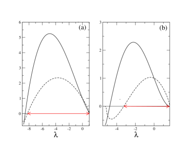
Figure 13: (Color on line) $\det\hat{C}^{l,+}_{w,antisym}(\lambda)/\det C$ (solid lines) and $\det(\hat{C}^{r,+}_{w,antisym}(\lambda)+C)/\det C$ (dashed lines) as a function of $\lambda$. The arrows indicate the range $\hat{\cal D}_{w}$ of values of $\lambda$ for which the matrices $\hat{C}^{l,+}_{w,antisym}(\lambda)$ and $\hat{C}^{r,+}_{w,antisym}(\lambda)+C$ are both positive definite (compare with Fig. 8). (a) $\tau=1$: ${\cal D}_{H}=(-472.08,1.019)$, $\hat{\cal D}_{w}=(-8.232,1.019)$. (b) $\tau=3$: ${\cal D}_{H}=(-5.118,1.665)$, $\hat{\cal D}_{w}(-3.235,1.612)$.

According to the recent work of du Buisson and Touchette (see Section III C of Ref. DBT2023 or Sec. 4.1.3 of Ref. DB2023 devoted to linear current-type observables), this symmetric component should be responsible for the reduction of the domain of existence of the SCGF from ${\cal D}_{H}$ to $\hat{\cal D}_{w}$. The results presented in Fig. 13, in which only the second term of Eq. (158) is taken into account, show that this is not true. The interval for which the matrices $\hat{C}^{l,+}_{w,antisym}(\lambda)$ and $\hat{C}^{r,+}_{w,antisym}(\lambda)+C$ are both positive definite is enlarged compared with the one associated with the full work $\beta{\cal W}_{t}$ (see Fig. 8) but it is still smaller than ${\cal D}_{H}$.

We believe that the problem with the analysis done in Ref. DBT2023 , which treats separately the cases where the matrix $B_{\rm o}$ is purely antisymmetric and that where it also has a nonzero symmetric part, is that it only focuses on the time evolution of the generating function $G^{r}_{\rm o,\lambda}({\bf u}_{0},t)$. As a result, the role of the matrix $\hat{C}^{l,+}_{\rm o}(\lambda)$ is not not clearly recognized, as we now briefly explain.

In the long-time limit, $G^{r}_{\rm o,\lambda}({\bf u}_{0},t)$ is given by Eq. (108a) which only involves the matrix $\hat{C}^{r,+}_{\rm o}(\lambda)$. However, $G^{r}_{\rm o,\lambda}({\bf u}_{0},t)$ results from the average of $G_{\rm o,\lambda}({\bf u},t|{\bf u}_{0})$ over the terminal state ${\bf u}$. Therefore, from Eq. (131), $G^{r}_{\rm o,\lambda}({\bf u}_{0},t)$ is finite if the left eigenfunction $l_{\rm o,\lambda}({\bf u})$ is integrable, which requires the matrix $\hat{C}^{l,+}_{\rm o}(\lambda)$ to be positive definite (this is why the determinant of $\hat{C}^{l,+}_{\rm o}(\lambda)$ appears in the expression (137a) of the right eigenfunction).

Surprisingly, the integration of $G_{\rm o,\lambda}({\bf u},t|{\bf u}_{0})$ over ${\bf u}$ is not taken into account in Sec. III C.1 of Ref. DBT2023 which considers the case of a purely antisymmetric matrix $B_{\rm o}$. It is only stated that the SCGF exists if the drift matrix of the effective process (cf. Eq. (65) in Ref. DBT2023 ) is positive definite. As we noted after Eq. (140), this condition is automatically satisfied when $\lambda\in{\cal D}_{H}$.

On the other hand, for a general matrix $B_{\rm o}$ (Sec. III C.2 of Ref. DBT2023 ), an additional condition is derived from the integral of $G_{\rm o,\lambda}({\bf u},t|{\bf u}_{0})$ over ${\bf u}$. A certain matrix, defined by Eq. (76), must be positive definite. Translated into our notations, this condition reads

$$[\hat{C}^{r,+}_{\rm o,antisym}(\lambda)+\hat{C}^{l,+}_{\rm o,antisym}(\lambda)]-\hat{C}^{r,+}_{\rm o,antisym}(\lambda)+\lambda B_{\rm o,sym}>0\ .$$ (160)

Using Eq. (92b), we see that it is just the condition $\hat{C}_{\rm o}^{l,+}(\lambda)>0$! So the positive definiteness of the matrix $\hat{C}_{\rm o}^{l,+}(\lambda)$ is always required, regardless of the symmetry of the matrix $B_{\rm o}$. Moreover, one may have $\hat{\cal D}_{w}\subset{\cal D}_{H}$ even if $B_{\rm o}$ is purely antisymmetric and no explicit boundary term is present. Note that this behavior is not specific to the present model: see, e.g., the two-dimensional model studied in Ref. NKP2013 where the matrix $B_{w}$ is purely antisymmetric or the model of a confined active particle studied in Ref. SGSZ2023 .

IV.3 Behavior of the SCGF at the limits of its interval of definition

As signaled by Eqs. (85) and illustrated numerically in Figs. 9 and 10, something special happens for the solutions of the RDEs at the boundaries of the interval $\hat{\cal D}_{\rm o}$ (throughout this section we assume that $\hat{\cal D}_{\rm o}\subset{\cal D}_{H}$ where we recall that $\subset$ denotes a strict inclusion). This may look as a minor issue, but we will see in Sec. V that it cannot be ignored in order to understand the behavior of the fluctuations of heat and entropy production for $\lambda=1$.

For concreteness we suppose hereafter that $\det\hat{C}^{l,+}_{\rm o}(\lambda_{\rm o1})=0$ and $\det(\hat{C}^{r,+}_{\rm o}(\lambda_{\rm o2})+C)=0$ like in the example of Fig. 8 (a similar discussion would take place in the opposite case). Eqs. (85) then tell us that $C^{r}_{\rm o}(\lambda_{\rm o1},t)\not\to\hat{C}^{r,+}_{\rm o}(\lambda_{\rm o1})$ and $C^{l}_{\rm o}(\lambda_{\rm o1},t)\to\hat{C}^{l,+}_{\rm o}(\lambda_{\rm o1})$ as $t\to\infty$ whereas $C^{l}_{\rm o}(\lambda_{\rm o2},t)\not\to\hat{C}^{l,+}_{\rm o}(\lambda_{\rm o2})$ and $C^{r}_{\rm o}(\lambda_{\rm o2},t)\to\hat{C}^{r,+}_{\rm o}(\lambda_{\rm o2})$. Therefore, there is a discontinuity in the solution of the RDE (42a) or (42b) and this naturally raises the question: What is the value of the SCGF for $\lambda=\lambda_{\rm o1}$ and $\lambda=\lambda_{\rm o2}$? We note that it is taken for granted in Ref. DBT2023 that the SCGF diverges (see Eq. (78); see also Eq. (4.104) in Ref. DB2023 ).

IV.3.1 Attraction to a non-extremal solution of the CARE

Consider for instance the behavior for $\lambda=\lambda_{\rm o1}$. We first treat the case where $C^{r}_{\rm o}(\lambda_{\rm o1},t)$, solution of the RDE (42a), converges and is attracted to a fixed point $\hat{C}_{\rm o}^{r,(\alpha)}(\lambda_{\rm o1})\neq\hat{C}_{\rm o}^{r,+}(\lambda_{\rm o1})$. This corresponds to the behavior observed in Fig. 10 where $\lim_{t\to\infty}\det(C^{r}_{w}(\lambda_{w1},t)+C)/\det C\approx 1.17$ whereas $\det(\hat{C}^{r,+}_{w}(\lambda_{w1})+C)/\det C\approx 2.98$. The asymptotic expression (108a) of the generating function $G^{r}_{\rm o,\lambda_{\rm o1}}({\bf u}_{0},t)$ is then replaced by

$$G^{r}_{\rm o,\lambda_{\rm o1}}({\bf u}_{0},t)\sim g^{r,(\alpha)}_{\rm o}(\lambda_{\rm o1})\exp\left(-\frac{1}{2}{\bf u}_{0}^{T}\hat{C}_{\rm o}^{r,(\alpha)}(\lambda_{\rm o1}){\bf u}_{0}\right)e^{f^{(\alpha)}(\lambda_{\rm o1})t}\ ,$$ (161)

where $f^{(\alpha)}(\lambda_{\rm o1})$ is given by Eq. (96) and

$$g^{r,(\alpha)}_{\rm o}(\lambda_{\rm o1})=\exp\left(\int_{0}^{\cal\infty}dt\>[f^{r}_{\rm o}(\lambda_{\rm o1},t)-f^{(\alpha)}(\lambda_{\rm o1})]\right)\ .$$ (162)

It remains to integrate $G^{r}_{\rm o,\lambda_{\rm o1}}({\bf u}_{0},t)p({\bf u}_{0})$ over ${\bf u}_{0}$. Whereas $\hat{C}^{r,+}_{\rm o}(\lambda_{\rm o1})+C>0$ by assumption, it is not guaranteed that $\hat{C}^{r,(\alpha)}_{\rm o}(\lambda_{\rm o1})+C>0$ because $\hat{C}^{r,(\alpha)}_{\rm o}(\lambda_{\rm o,1})<\hat{C}^{r,+}_{\rm o}(\lambda_{\rm o,1})$. If this positivity condition is not satisfied, the integral diverges and the SCGF is infinite for $\lambda=\lambda_{\rm o1}$. On the other hand, if $\hat{C}^{r,(\alpha)}_{\rm o}(\lambda_{\rm o1})+C>0$, as is the case in the example of Fig. 10, one finds

$$G_{\rm o,\lambda_{\rm o1}}(t)\sim g_{\rm o}(\lambda_{\rm o1})e^{f^{(\alpha)}(\lambda_{\rm o1})t}\ ,$$ (163)

with

$$g_{\rm o}(\lambda_{\rm o1})=\Big{[}\frac{\det\big{(}C+\hat{C}^{r,(\alpha)}_{\rm o}(\lambda_{\rm o1})\big{)}}{\det C}\Big{]}^{-1/2}\exp\left(\int_{0}^{\cal\infty}dt\>[f^{r}_{\rm o}(\lambda_{\rm o1},t)-f^{(\alpha)}(\lambda_{\rm o1})]\right)\ .$$ (164)

In consequence, the SCGF $\mu_{\rm o}(\lambda_{\rm o1})$ is finite and equal to $f^{(\alpha)}(\lambda_{\rm o1})$. Furthermore, since $f^{(\alpha)}(\lambda_{\rm o1})>f^{+}(\lambda_{\rm o1})$ [Eq. (101)], the SCGF exhibits a positive jump discontinuity at $\lambda=\lambda_{\rm o1}$. Note also that the actual pre-exponential factor $g_{\rm o}(\lambda_{\rm o1})$ is finite.

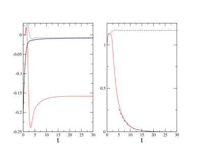
Figure 14: (Color on line) Time evolution of the solutions of the RDEs (42) for the observable ${\cal W}_{t}$ for $\tau=1$ and $\lambda=\lambda_{w1}\approx-0.9635155087944421810$. (a) $f_{w}^{l}(\lambda_{w1},t)$ (red solid line), $f_{w}^{r}(\lambda_{w1},t)$ (blue dashed line), $(1/t)\ln G_{w}(\lambda_{w1},t)$ (black solid line). (b) $\det C_{w}^{l}(\lambda_{w1},t)/\det C$ (red solid line) and $\det(C_{w}^{r}(\lambda_{w,1},t)+C)/\det C$ (blue dashed line). The dashed-dotted black line represents the fit $1.26\exp(-0.302t)$ to $\det C_{w}^{l}(\lambda_{w1},t)/\det C$ for $t>10$.

How can this result be compatible with that obtained by integrating $G^{l}_{\rm o,\lambda_{\rm o1}}({\bf u},t)$ over the final state ${\bf u}$? The long-time behavior of $G^{l}_{\rm o,\lambda_{\rm o1}}({\bf u},t)$ is still described by Eq. (108b) but $\det C^{l}_{\rm o}(\lambda_{\rm o1},t)\to\det\hat{C}^{l,+}_{\rm o}(\lambda_{\rm o1})=0$, which makes the expression (111b) of the pre-exponential factor divergent. To resolve the puzzle one must go back to the expression (48b) of the generating function and carefully inspect the long-time behavior of the solution of the RDE (42b). It is then found that $\det C^{l}_{\rm o}(\lambda_{\rm o1},t)\sim e^{-2\delta t}$ with $\delta=f^{(\alpha)}(\lambda_{\rm o1})-f^{+}(\lambda_{\rm o1})>0$. As $t\to\infty$, the factor $e^{f^{+}(\lambda_{\rm o1})t}$ in the denominator of Eq. (48b) then cancels the same factor in the numerator that comes from the limit of $e^{\int_{0}^{t}f^{l}_{\rm o}(\lambda_{\rm o1},t)dt}$, and one eventually recovers that $\mu_{\rm o}(\lambda_{\rm o1})=f^{(\alpha)}(\lambda_{\rm o1})$, as it must be.

This nontrivial behavior is illustrated numerically in Fig. 14 for the observable ${\cal W}_{t}$ and the same parameters as in Figs. 8(a), 9, and 10. Note that there is no explicit expression of $\lambda_{w1}$ so that its numerical value is only known approximately by solving the equation $\det C_{w}^{l+}(\lambda_{w1})=0$. As a result, the solution of the RDE (42a) is ultimately attracted to $\hat{C}_{w}^{r,+}(\lambda_{w1})$ and a very high precision in the determination of $\lambda_{w1}$ is required to observe the convergence to $\hat{C}_{w}^{r,(\alpha)}(\lambda_{w1})$ within a sufficiently large time window. Then, we see in Fig. 14(a) that the function $f_{w}^{l}(\lambda_{w1},t)$ converges to $f^{+}(\lambda_{w1})\simeq-0.158$ whereas both $f_{w}^{r}(\lambda_{w1},t)$ and $(1/t)\ln G_{w,\lambda_{w1}}(t)$ converge to $f^{(\alpha)}(\lambda_{w1})\simeq-0.007$ which is thus the actual value of the SCGF $\mu_{w}(\lambda_{w1})$. We also observe that $2[f^{+}(\lambda_{w1})-f^{(\alpha)}(\lambda_{w1}]\approx-0.302$, which is in perfect agreement with the exponential fit to $\det C_{w}^{l}(\lambda_{w1},t)/\det C$ shown in Fig. 14(b) and confirms the theoretical analysis. The discontinuity in the SCGF for $\lambda=\lambda_{w1}$ (which does not contradict the required convexity of the SCGF T2009 since $\mu_{w}(\lambda)=+\infty$ for $\lambda<\lambda_{w1}$)) signals an abrupt change in the mechanism responsible for the fluctuations of ${\cal W}_{t}$ which can interpreted as a dynamical phase transition.

More generally, one may wonder whether the exceptional value $f^{(\alpha)}(\lambda_{\rm o1})\neq f^{+}(\lambda_{\rm o1})$ of the SCGF could also be obtained by solving the spectral problem

$${\cal L}_{\rm o,\lambda_{\rm o1}}r_{\rm o,\lambda_{\rm o1}}({\bf u}_{0}) =f^{(\alpha)}(\lambda_{\rm o1})r_{\rm o,\lambda_{\rm o1}}({\bf u}_{0})$$ (165a)

$${\cal L}_{\rm o,\lambda_{\rm o1}}^{{\dagger}}\,l_{\rm o,\lambda_{\rm o1}}({\bf u}) =f^{(\alpha)}(\lambda_{\rm o1})l_{\rm o,\lambda_{\rm o1}}({\bf u})\ ,$$ (165b)

with $r_{\rm o,\lambda}({\bf u}_{0})=g_{\rm o}^{r}(\lambda_{\rm o1})\exp\left(-\frac{1}{2}{\bf u}_{0}^{T}\hat{C}^{r,(\alpha)}_{\rm o}(\lambda_{\rm o1}){\bf u}_{0}\right)$ and $g_{\rm o}^{r}(\lambda_{\rm o1})$ given by Eq. (162). This requires the existence of a left eigenfunction $l_{\rm o,\lambda_{\rm o1}}({\bf u})$ such that the normalization conditions (133) are satisfied. If so, the driven process is again a linear diffusion with a drift matrix given by Eq. (140). The invariant density is thus a multidimensional Gaussian and the left eigenfunction is also Gaussian from Eq. (141). In other words, one must have $l_{a,\lambda}({\bf u}_{0})=g_{\rm o}^{l}(\lambda_{\rm o1})\exp\left(-\frac{1}{2}{\bf u}^{T}\hat{C}^{l,(\alpha)}_{\rm o}(\lambda_{\rm o1}){\bf u}\right)$ and the problem thus amounts to computing the matrix $\hat{C}^{l,(\alpha)}_{\rm o}(\lambda_{\rm o1})$ and checking whether the normalization conditions are satisfied.

One first needs to identify the corresponding set ${\cal S}_{\lambda_{\rm o1}}^{(\alpha)}$ of eigenvalues of the Hamiltonian matrices. To be concrete, let us take the same example as in Fig. 14. For these values of the parameters, we find that all eigenvalues of the Hamiltonian matrices are simple with $3$ pairs of complex conjugate eigenvalues $(s_{1}^{+},\bar{s}_{1}^{+})$, $(s_{2}^{+},\bar{s}_{2}^{+})$, $(s_{3}^{+},\bar{s}_{3}^{+}$) and one real eigenvalue $s_{4}^{+}$ on the r.h.s. of the complex plane ($s_{4}^{+}$ is the eigenvalue with the smallest real part). The CARE (86a) has thus $16$ real, symmetric solutions note7 , and by using Eq. (96) we find that the value $f^{(\alpha)}(\lambda_{w1})\approx-0.007$ is obtained from the set ${\cal S}_{\lambda_{w,1}}^{(\alpha)}=\{s_{1}^{+},\bar{s}_{1}^{+},s_{2}^{+},\bar{s}_{2}^{+},s_{3}^{+},\bar{s}_{3}^{+},s_{4}^{-}\}$ with $s_{4}^{-}=-s_{4}^{+}$. This allows us to compute the corresponding matrix $\hat{C}^{l,(\alpha)}_{w}(\lambda_{w1})$. We then observe that neither $\hat{C}^{l,(\alpha)}_{w}(\lambda_{\rm o,1})$ nor $\hat{C}^{r,(\alpha)}_{w}(\lambda_{w1})+\hat{C}^{l,(\alpha)}_{w}(\lambda_{w1})$ are positive definite. Hence $\hat{C}^{l,(\alpha)}_{w}(\lambda_{w1})$ is not an acceptable eigenfunction and we conclude that the SCGF cannot be obtained from the spectral problem. We believe that this is a general feature although we have not been able to prove this conjecture so far.

IV.3.2 Oscillatory behavior

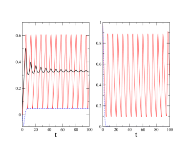
Figure 15: (Color on line) Time evolution of the solutions of the RDEs (42) for the observable ${\cal W}_{t}$ for $\tau=0.2$ and $\lambda=\lambda_{w2}\approx 0.3998261896653990830031041$. (a) $f_{w}^{l}(\lambda,t)$ (red solid line), $f_{w}^{r}(\lambda,t)$ (blue dashed line), $(1/t)\ln G_{w}(\lambda_{w2},t)$ (black solid line). (b) $\det C_{w}^{l}(\lambda_{w2},t)/\det C$ (red solid line) and $\det(C_{w}^{r}(\lambda_{w2},t)+C)/\det C$ (blue dashed line).

Another possible scenario is that the solution of the RDE does not converge at all for $\lambda=\lambda_{\rm o1}$ or $\lambda=\lambda_{\rm o2}$. Suppose for instance that $\det(\hat{C}^{l,+}_{\rm o}(\lambda_{\rm o2})\neq 0$ and $\det(\hat{C}^{r,+}_{\rm o}(\lambda_{\rm o2})+C)=0$. As illustrated in Fig. 15 for $\rm o=w$ and $\tau=0.2$, $C^{r}_{w}(\lambda_{w2},t)\to\hat{C}^{r,+}(\lambda_{w2})$ with $f^{r}(\lambda_{w2},t)\to f^{+}(\lambda_{w2})\approx 0.047$ whereas $C^{l}_{w}(\lambda_{w2},t)$, after some short transient, oscillates between $\hat{C}^{l,+}(\lambda_{w2})$ and another fixed point $\hat{C}^{l,(\alpha)}(\lambda_{w2})$ corresponding to $f^{(\alpha)}(\lambda_{w2})\approx 0.607$ [see Fig. 15(a)]. More precisely, it is observed that each element of the matrix $C^{l}_{w}(\lambda_{w2},t)$ behaves as

$$[C^{l}_{w}(\lambda_{w2},t)]_{ij}\sim[\hat{C}^{l,+}_{w}(\lambda_{w2})]_{ij}\frac{1+h(t+\delta_{ij})}{2}+[\hat{C}^{l,(\alpha)}_{w}(\lambda_{w2})]_{ij}\frac{1-h(t+\delta_{ij})}{2}\ ,$$ (166)

where $h(t)$ is a periodic function varying between $-1$ and $+1$ and $\delta_{ij}$ is a phase shift. This yields from Eq. (40b)

$$G^{l}_{w,\lambda_{\rm o2}}({\bf u},t)\sim g^{l}_{w}(\lambda_{w2})\exp\left(-\frac{1}{2}{\bf u}^{T}C^{l}_{w}(\lambda_{w2},t){\bf u}\right)e^{\bar{f}(\lambda_{w2})t}\ ,$$ (167)

with

$$g^{l}_{w}(\lambda_{w2})=\exp\left(\int_{0}^{\cal\infty}dt\>[f^{l}_{w}(\lambda_{w2},t)-\bar{f}(\lambda_{w2})]\right)\ ,$$ (168)

and

$$\bar{f}(\lambda_{w2})=f^{+}(\lambda_{w2})\frac{1+\bar{h}}{2}+f^{(\alpha)}(\lambda_{w2})\frac{1-\bar{h}}{2}\ ,$$ (169)

where $\bar{h}$ is the average of $h(t)$ over a single period. Since $\det C^{l}_{w}(\lambda_{w2},t)>0$ [see Fig. 15(b)], the integral of $G^{l}_{w,\lambda_{w2}}({\bf u},t)$ over ${\bf u}$ then yields

$$G_{w,\lambda_{w2}}(t)\sim g_{w}(\lambda_{w2},t)e^{\bar{f}(\lambda_{w2})t}\ ,$$ (170)

with

$$g_{w}(\lambda_{w2},t)=\big{[}\frac{\det C^{l}_{w}(\lambda_{w2},t)}{\det C}\Big{]}^{-1/2}\exp\left(\int_{0}^{\infty}dt\>[f^{l}_{w}(\lambda_{w2},t)-\bar{f}(\lambda_{w2})]\right)\ .$$ (171)

As can be seen in Fig. 15(a), the generating function exhibits decreasing oscillations and $(1/t)\ln G_{w,\lambda_{w2}}(t)\to\bar{f}(\lambda_{w2})\approx 0.33$, which is the genuine value of the SCGF. Moreover, the sub-exponential factor is time-dependent, which is an unusual feature. As it must be, the same result is obtained from the RDE (48a), with $C^{r}_{w}(\lambda_{w2},t)\to\hat{C}^{r,+}(\lambda_{w2})$. This is due again to the fact that the determinant of $C^{r}_{w}(\lambda_{w2},t)+C$ decreases exponentially to $0$ as $t\to\infty$ in a very specific way.

V The special case $\lambda=1$

In this final section, we study the special case $\lambda=1$ in relation with the fluctuation relations for the heat ${\cal Q}_{t}$ and the (apparent) entropy production $\Sigma_{t}$. This is an important application of the general formalism described in the preceding sections and it also motivates our focus on the behavior of the SCGF at the limits of its domain of definition. For concreteness, we restrict our attention to the model with distributed time delay described by Eq. (4).

V.1 Preliminaries

A first observation is that the characteristic polynomial of the Hamiltonian matrices for $\lambda=1$ admits the factorization

$$p_{H}(1,s)=(-1)^{n}q^{*}(s)q^{*}(-s),$$ (172)

with

$$q^{*}(s)=(-\frac{n}{\tau})^{n}[(s^{2}+\frac{s}{Q_{0}}+1)(1-\frac{s\tau}{n})^{n}-\frac{g}{Q_{0}}]\ .$$ (173)

This results from simple manipulations of Eq. (72). From the general property of algebraic Riccati equations [Eq. (112)], this factorization indicates that there exist a symmetric matrix $\hat{C}^{r,*}_{\rm o}(1)$, solution of the CARE (86a), and a symmetric matrix $\hat{C}^{l,*}_{\rm o}(1)$, solution of the CARE (86b), such that $q^{*}(s)$ is the characteristic polynomial of $-A_{\rm o}(1)+D\hat{C}^{r,*}_{\rm o}(1)$ and $A_{\rm o}(1)+D\hat{C}^{l,*}_{\rm o}(1)$. The matrices $\hat{C}^{r,*}_{\rm o}(1)$ and $\hat{C}^{l,*}_{\rm o}(1)$ are associated with the subset ${\cal S}^{*}=\{s^{*}_{1},s^{*}_{2},...s^{*}_{n+2}\}$ of eigenvalues of the Hamiltonian matrices composed of the $n+2$ roots of $q^{*}(s)$.

From Eq. (173) we have

$$q^{*}(s)=s^{n+2}+s^{n+1}(\frac{1}{Q_{0}}-\frac{n^{2}}{\tau})+...\ ,$$ (174)

so that

$$\sum_{i}^{n+2}s^{*}_{i}=\frac{n^{2}}{\tau}-\frac{1}{Q_{0}}$$ (175)

and from Eq. (96),

$$f^{*}(1)=-\frac{1}{2}[\mbox{Tr}(A)+\sum_{i}^{n+2}s_{i}^{*}]=\frac{1}{Q_{0}}\,.$$ (176)

It then follows from Eqs. (94) that

$$[\hat{C}^{r,*}_{\rm o}(1)]_{11}=-\frac{2}{Q_{0}}-[S_{\rm o}]_{11}$$ (177a)

$$[\hat{C}^{l,*}_{\rm o}(1)]_{11}=\frac{2n^{2}}{\tau}+[S_{\rm o}]_{11}\ ,$$ (177b)

and by inspecting the CARE (86a) we discover that the only solution satisfying Eq. (177a) is the matrix

$$\hat{C}^{r,*}_{\rm o}(1)=S_{q}-S_{\rm o}\ .$$ (178)

Hence $q^{*}(s)$ is just the characteristic polynomial of $-A_{\rm o}(1)+D(S_{q}-S_{\rm o})=-A+DS_{q}$, as can be verified explicitly. On the other hand, no simple expression of the matrix $\hat{C}^{l,*}_{\rm o}(1)$ is available.

In consequence two cases may occur:

$\bullet$ Case (a): All roots of $q^{*}(s)$ have a positive real part, i.e, ${\cal S}^{*}_{1}={\cal S}_{1}^{+}$ and $q^{+}(1,s)=q^{*}(s)$ (note that Eq. (175) implies that this case does not exist if $\tau/Q_{0}>n^{2}$). Then,

$$\hat{C}_{\rm o}^{r,+}(1)=\hat{C}^{r,*}_{\rm o}(1)$$ (179)

and

$$f^{+}(1)=f^{*}(1)=\frac{1}{Q_{0}}\ .$$ (180)

Furthermore, if $\hat{C}^{r,+}_{\rm o}(1)+C>0$ and $\hat{C}^{l,+}_{\rm o}(1)>0$ (i.e., $\lambda=1\in\hat{\cal D}_{\rm o}$) so that the effective process exists for the observable $\rm o$, this process takes a remarkable form. Since $\hat{C}_{w}^{r,+}(1)=S_{q}$, Eq. (147) indeed becomes

$$\dot{v}(t)=\frac{1}{Q_{0}}v(t)-x(t)+\frac{g}{Q_{0}}\int_{-\infty}^{t}ds\>g_{n}(t-s,n/\tau)x_{s}+\xi(t)\ .$$ (181)

Therefore, atypical fluctuations of the observable are created in the long-time limit by simply changing the sign of the friction coefficient in the original Langevin dynamics (see also Ref. RTM2017 ). Moreover, for $\rm o=w$, an analysis similar to the one performed in Sec. IIIB and Appendix A of Ref. RTM2017 shows that the pre-exponential factor $g_{w}(1)$ is given by

$$g_{w}(1)=\frac{1}{\sqrt{(1-\frac{T_{x}}{T})(1-\frac{T_{v}}{T})(1+\frac{\hat{T}_{x}(1)}{T})(1+\frac{\hat{T}_{v}(1)}{T})}}\ .$$ (182)

According to the identity (61) the condition $\hat{C}^{r,+}_{w}(1)+C=S_{q}+C>0$ requires that the temperatures $T_{x}$ and $T_{v}$ are both strictly smaller or both strictly larger than the bath temperature $T$. This ensures that Eq. (182) gives a real result. We stress again that this simple and remarkable expression only holds in case (a).

$\bullet$ Case (b): Some roots of $q^{*}(s)$ have a negative real part, i.e., ${\cal S}^{(\tilde{\alpha})}_{1}\neq{\cal S}_{1}^{+}$ and $q^{+}(1,s)\neq q^{*}(s)$ . Then,

$$\hat{C}_{\rm o}^{r,+}(1)>\hat{C}^{r,*}_{\rm o}(1)$$ (183)

since $\hat{C}_{\rm o}^{r,+}(1)$ is the maximal solution of the CARE (86a), and

$$f^{+}(1)=\frac{1}{Q_{0}}+\sum_{i}s_{i}^{*-}<\frac{1}{Q_{0}}\ ,$$ (184)

where the sum runs over all roots of $q^{*}(s)$ with a negative real part [cf. Eq. (IV.2.2)].

For given values of $Q_{0}$ and $g$, case (a) typically takes place in a limited range of values of $\tau$. This is illustrated in Fig. 16(a) where $f^{+}(1)$ is plotted as a function of $\tau$ (we recall that for this choice of the parameters the system reaches a stable stationary state for all values of $\tau$). Here, $f^{+}(1)=1/Q_{0}$ for $\tau_{1}\leq\tau\leq\tau_{2}$ with $\tau_{1}\approx 0.71$ and $\tau_{2}\approx 1.77$. We also display in Fig. 16(b) the corresponding kinetic temperature $\hat{T}_{v}(1)=2/Q_{0}\langle v^{2}\rangle_{\lambda=1}$ computed from Eq. (154b) which characterizes the stationary distribution of the effective process together with $\hat{T}_{x}(1)$. Note that these temperatures diverge for $\tau=\tau_{1}$ and $\tau=\tau_{2}$ since a pair of roots of $p_{H,1}(s)$ becomes purely imaginary and thus $\lambda_{\max}=1$ (this is also true for all components of the covariance matrix $\hat{\Sigma}(1)$ except $[\hat{\Sigma}(1)]_{12}=\langle vx\rangle_{\lambda=1}=0$).

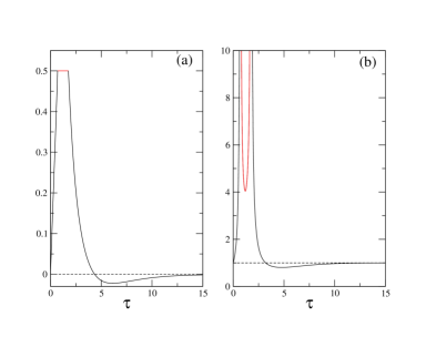
Figure 16: (Color on line) (a) $f^{+}(1)$ as a function of $\tau$ for $Q_{0}=2,g=1.5$ and $n=5$. One has $f^{+}(1)=1/Q_{0}$ for $0.70\lesssim\tau\lesssim 1.77$ (in red). (b) Corresponding stationary kinetic temperature $\hat{T}_{v}(1)$ of the effective process.

V.2 Integral fluctuation theorem (IFT) for the heat

As pointed out at the end of Sec. III.1, the solution of the RDE (42a) with initial condition $C^{r}_{q}(1,0)=0$ is $C^{r}_{q}(1,t)=0$ owing to the fact that $K_{q}(1)=0$. As a result, $f_{q}^{r}(1,t)=1/Q_{0}$ from Eq. (47a) and one recovers the universal IFT $\langle e^{-\beta{\cal Q}_{t}}\rangle=e^{t/Q_{0}}$ for the fluctuating heat in underdamped Langevin processes RTM2016 . In particular, the SCGF is equal to $1/Q_{0}$ and is associated with the matrix $\hat{C}_{q}^{r,*}(1)=0$ in agreement with Eq. (178) above. In addition, $g_{q}(1)=1$.

It is instructive to examine how this exact result is recovered from the solution of the RDE (42b) for the matrix $C^{l}_{q}(1,t)$. According to Eqs. (179) and (183), the matrix $\hat{C}^{r,+}_{q}(1)$ is positive semidefinite. Hence, $C+\hat{C}^{r,+}_{q}(1)>0$, which implies that $C^{l}_{q}(1,t)\to\hat{C}_{q}^{l,+}(1)$ in both cases (a) and (b). However, the corresponding scenarios are different.

$\bullet$ Case (a): One has $\hat{C}_{q}^{r,+}(1)=\hat{C}_{q}^{r,*}(1)=0$ from Eq. (179) and, thus, $\hat{C}_{q}^{r,+}(1)$ is the trivial (i.e., zero) asymptotic fixed point of the RDE (42a). Then $\hat{C}^{l,+}_{q}(1)$ is also associated with the SCGF $f^{+}(1)=1/Q_{0}$ and $\det\hat{C}^{l,+}_{q}(1)\neq 0$. Furthermore, from Eq. (136), $g_{q}(1)=1$. In short, $\lambda=1$ is in interior of the interval $\hat{\cal D}_{q}$ and the SCGF $\mu_{q}(\lambda)$ is regular at $\lambda=1$.

$\bullet$ Case (b): $\hat{C}_{q}^{r,+}(1)>\hat{C}_{q}^{r,*}(1)=0$ and $f^{+}(1)<1/Q_{0}$ according to Eqs. (183) and (184). Since $\hat{C}_{q}^{l}(1,t)\to\hat{C}_{q}^{l,+}(1)$ but $\hat{C}_{q}^{r}(1,t)=0\not\to\hat{C}_{q}^{r,+}(1)$, one must have $\det\hat{C}^{l,+}_{q}(1)=0$, and the scenario is the one described in Sec. IV.3.1 with $\lambda_{q2}=1$. In particular, $\det C^{l}_{q}(1,t)\sim e^{-2t[1/Q_{0}-f^{+}(1)]}$ as $t\to\infty$ so that the actual value $1/Q_{0}$ of the SCGF is recovered. The SCGF $\mu_{q}(\lambda)$ then displays a positive jump discontinuity at $\lambda=1$, which is the upper limit of its domain of definition, and the rate function $I_{q}(a)$ has a linear tail for $a\leq a^{-}=-df^{+}(\lambda)/d\lambda|_{\lambda=1}$.

V.3 Asymptotic fluctuation relation for the entropy production

V.3.1 Acausal dynamics and Jacobian

As pointed out in Ref. RMT2015 , the microscopic reversibility condition (or local detailed balance) that links dissipation to time-reversal symmetry breaking S2012 ; K1998 ; C1998 ; LS1999 ; MN2003 ; G2004a is not satisfied by a Langevin dynamics with a time-delayed continuous feedback. On the other hand, local detailed balance is recovered if the time-reversal operation is combined with the change $\tau\to-\tau$. Although this procedure is purely mathematical, it was used in our previous studies to derive a second-law-like inequality for the extracted work rate in the stationary state (see Eq. (84) in Ref. RMT2015 ) and to predict that

$$\mu_{\sigma}(1)\equiv\lim_{t\to\infty}(1/t)\ln\langle e^{-\Sigma_{t}}\rangle=\dot{\cal S}_{\cal J}\equiv\lim_{t\to\infty}\frac{1}{t}\langle\ln\frac{{\cal J}_{t}}{\widetilde{\cal J}_{t}}\rangle\ ,$$ (185)

where ${\cal J}_{t}$ is the Jacobian of the transformation $\xi(t)\to x(t)$ associated with Eq. (3) and $\widetilde{\cal J}_{t}$ is the Jacobian associated with the corresponding acausal Langevin equation in which $\tau$ is changed into $-\tau$ MR2014 ; RMT2015 ; RTM2017 . If true, Eq. (185) is remarkable since the left-hand side is a quantity that can be extracted from numerical simulations of Eq. (3) RTM2017 ; MR2014 or from experiments DRLK2022 whereas the quantity on the right-hand side is associated with a dynamics that is not physically realizable. Our objective in the following is to compute the explicit expression of $\mu_{\sigma}(1)$ for an arbitrary value of $n$ via the Riccati-based approach and to show that it is indeed identical to the expression of $\dot{\cal S}_{\cal J}$ when this latter quantity exists.

For the sake of conciseness, we will not repeat here the lengthy analysis performed in Ref. RMT2015 that yielded the expression of $\dot{\cal S}_{\cal J}$ for the discrete delay (i.e., for $n=\infty$). The main steps of the calculation for $n$ finite are similar and we refer the interested reader to this previous article. The outcome is the integral formula

$$\dot{\cal S}_{\cal J}=\frac{1}{2\pi i}\int_{c-i\infty}^{c+i\infty}ds\>\ln\frac{\widetilde{\chi}_{n}(s)}{\chi_{g=0}(s)}\ ,$$ (186)

where

$$\chi_{g=0}(s)=[s^{2}+\frac{s}{Q_{0}}+1]^{-1}$$ (187)

is the response function of the system in the absence of feedback and

$$\widetilde{\chi}_{n}(s)=[s^{2}+\frac{s}{Q_{0}}+1-\frac{g}{Q_{0}}(1-\frac{s\tau}{n})^{-n}]^{-1}\ .$$ (188)

The integration in Eq. (186) is performed along the vertical line $\mbox{Re}(s)=c$ and a careful study of the branch cuts of the multivalued function $\ln[\widetilde{\chi}_{n}(s)/\chi_{g=0}(s)]$ in the complex $s$-plane shows that $c$ must be chosen such that two and only two poles of $\widetilde{\chi}_{n}(s)$, hereafter denoted by $s^{*}_{1}$ and $s^{*}_{2}$, are located on the left side of the line $\mbox{Re}(s)=c$. An integration contour similar to the one displayed in Fig. 4 of Ref. RMT2015 then leads to the simple expression

$$\dot{\cal S}_{\cal J}=\frac{1}{Q_{0}}+(s^{*}_{1}+s^{*}_{2})\ .$$ (189)

As discussed in Refs. RMT2015 ; RTM2017 , $\widetilde{\chi}_{n}(s)$ may be viewed as the bilateral Laplace transform of the response function associated with the acausal dynamics, and in analogy with Eq. (123) it can be also expressed as

$$\widetilde{\chi}_{n}(s)=\frac{(s-\frac{n}{\tau})^{n}}{\widetilde{p}_{A}(s)}\ ,$$ (190)

where $\widetilde{p}_{A}(s)\equiv p_{A}^{\tau\to-\tau}(s)$ [see Eq. (24)]. In fact, $\widetilde{p}_{A}(s)$ is nothing but $q^{*}(s)$, the polynomial introduced in Sec. V.1 [Eq. (173)]. In consequence, $s^{*}_{1}$ and $s^{*}_{2}$ are roots of $q^{*}(s)$, and by comparing with Eq. (184) we deduce that

$$\bullet\>\mbox{(a)}\>\>\>\dot{\cal S}_{\cal J}>f^{+}(1)=1/Q_{0}\>\>\mbox{if all roots of $q^{*}(s)$ have a positive real part ($c>0$)}$$ (191a)

$$\bullet\>\mbox{(b1)}\>\>\>\dot{\cal S}_{\cal J}=f^{+}(1)<1/Q_{0}\>\>\mbox{if exactly two roots of $q^{*}(s)$ have a negative real part ($c=0$)}$$ (191b)

$$\bullet\>\mbox{(b2)}\>\>\>f^{+}(1)<\dot{\cal S}_{\cal J}<1/Q_{0}\>\>\mbox{if more than two roots of $q^{*}(s)$ have a negative real part ($c<0$)}\ .$$ (191c)

As will be seen in the following, there is also a fourth case that was missed in Ref. RMT2015 : If the root of $q^{*}(s)$ with the smallest real part is real and the next roots are complex conjugate, the Bromwich contour $\mbox{Re}(s)=c$ cannot be defined and Eq. (186) breaks down (which simply means that $\mu_{\sigma}(1)$ does not exist).

Before embarking into the (rather lengthy) proof that $\mu_{\sigma}(1)$ (when it exists) is also given by Eq. (189), let us make a short remark about the acausal dynamics. Despite the unphysical character of this dynamics, a steady state can still be defined if the response function $\widetilde{\chi}_{n}(t)$ in the time domain decreases sufficiently fast to zero for both $t\to+\infty$ and $t\to-\infty$ (see the discussion in Appendix A of Ref. RTM2017 ). This requires that $q^{*}(s)$ has only two roots with a negative real part (case (b1) above). The steady state is then characterized by a multivariate Gaussian distribution with a covariance matrix $\widetilde{\Sigma}$ whose elements are given by [see Eqs. (150) and (151)]

$$\widetilde{\Sigma}_{ij}=\int\frac{d\omega}{2\pi}\widetilde{R}_{i,1}(\omega)\widetilde{R}_{j,1}(-\omega)\ ,$$ (192)

where

$$\widetilde{R}(\omega)=-[\widetilde{A}+i\omega I_{n+2}]^{-1}$$ (193)

and $\widetilde{A}\equiv A^{\tau\to-\tau}$. In particular, one has

$$\frac{\widetilde{T}_{x}}{T} =\frac{2}{Q_{0}}\widetilde{\Sigma}_{22}=\frac{2}{Q_{0}}\int\frac{d\omega}{2\pi}|\widetilde{\chi}_{n}(\omega)|^{2}$$ (194a)

$$\frac{\widetilde{T}_{v}}{T} =\frac{2}{Q_{0}}\widetilde{\Sigma}_{11}=\frac{2}{Q_{0}}\int\frac{d\omega}{2\pi}\omega^{2}|\widetilde{\chi}_{n}(\omega)|^{2}\ .$$ (194b)

Using Eq. (190) and the fact that $\widetilde{p}_{A}(s)\widetilde{p}_{A}(-s)=q^{*}(s)q^{*}(-s)=(-1)^{n}p_{H}(1,s)$, it is readily seen that these temperatures coincide with the temperatures $\hat{T}_{x}(1)$ and $\hat{T}_{v}(1)$ characterizing the stationary density associated with the effective process [see Eqs. (154)]. On the other hand, it is found that $\widetilde{\Sigma}_{n+2,1}=-\hat{\Sigma}_{n+2,1}(1)$ [with $\hat{\Sigma}_{n+2,1}(1)$ given by Eq. (IV.2.4)]. The negative sign indicates that the acausal dynamics does not generate the trajectories leading to a given fluctuation of the time-intensive observable $(2g/Q_{0}^{2})(1/t)\int_{0}^{t}dt^{\prime}x_{n}(t^{\prime})\circ dx(t^{\prime})$. Therefore, this dynamics must not be misinterpreted as being the effective process, as was done in Sec. IVB4 of Ref. RTM2017 .

V.3.2 Calculation of the SCGF

Let us assume that the matrix $C^{l}_{\sigma}(1,t)$ is nonsingular at all times so that its inverse $\Sigma^{l}_{\sigma}(1,t)$ exists. To prove that $\mu_{\sigma}(1)=\dot{\cal S}_{\cal J}$, it will be convenient to work with the expression of $G_{\sigma,1}(t)$ given by Eq. (49), that is

$$G_{\sigma,1}(t) =\exp\left(-\frac{1}{2}\int_{0}^{t}\mbox{Tr}\big{[}K_{\sigma}(1)\Sigma^{l}_{\sigma}(1,t^{\prime})+DB_{\sigma}\big{]}dt^{\prime}\right)\ ,$$ (195)

where $\Sigma^{l}_{\sigma}(1,t)$ satisfies the complementary RDE

$$\dot{\Sigma}^{l}_{\sigma}(1,t)=A_{\sigma}(1)\Sigma^{l}_{\sigma}(1,t)+\Sigma^{l}_{\sigma}(1,t)A^{T}_{\sigma}(1)-\Sigma^{l}_{\sigma}(1,t)K_{\sigma}(1)\Sigma^{l}_{\sigma}(1,t)+D$$ (196)

with initial condition $\Sigma^{l}_{\sigma}(1,0)=\Sigma$. It turns out that Eq. (195) can be greatly simplified by introducing the inverse of the matrix $X_{\sigma}^{l}(1,t)\equiv C_{\sigma}^{l}(1,t)-S_{\sigma}$. Due to the invariance property (54), $X_{\sigma}^{l}(1,t)$ is solution of the RDE

$$\dot{X}_{\sigma}^{l}(1,t)=-AX_{\sigma}^{l}(1,t)-X_{\sigma}^{l}(1,t)A^{T}-X_{\sigma}^{l}(1,t)DX_{\sigma}^{l}(1,t)+K_{w}(1)$$ (197)

with initial condition $X_{\sigma}^{l}(1,0)=C-S_{\sigma}$ while its inverse, which is simply denoted $Y(t)$ hereafter, is solution of the complementary RDE

$$\dot{Y}(t)=AY(t)+Y(t)A^{T}-Y(t)K_{w}(1)Y(t)+D$$ (198)

with initial condition $Y(0)=(C-S_{\sigma})^{-1}$. Note that the fact that $X_{\sigma}^{l}(1,t)$ is invertible results from the assumption that $\Sigma_{\sigma}^{l}(1,t)$ exists. Indeed, inspection of Eq. (196) shows that $[\Sigma^{l}_{\sigma}(1,t)]_{11}=\Sigma_{11}=(Q_{0}/2)T_{v},[\Sigma^{l}_{\sigma}(1,t)]_{22}=\Sigma_{22}=(Q_{0}/2)T_{x}$ and $[\Sigma^{l}_{\sigma}(1,t)]_{12}=\Sigma_{12}=0$, which, together with the definition of the matrix $S_{\sigma}$, yields

$$\det\big{(}I_{n+2}-S_{\sigma}\Sigma^{l}_{\sigma}(1,t)\big{)}=\frac{T_{x}T_{v}}{T^{2}}\,.$$ (199)

As a result,

$$\det(C_{\sigma}^{l}(1,t)-S_{\sigma})=\frac{T_{x}T_{v}}{T^{2}}\det C^{l}_{\sigma}(1,t)\neq 0\ .$$ (200)

The matrix $Y(t)$, solution of Eq. (198), has two remarkable properties:

(i) the elements $Y_{11}(t),Y_{22}(t)$ and $Y_{12}(t)$ are constant, with $Y_{11}(t)=Y_{22}(t)=Q_{0}/2$ and $Y_{12}(t)=0$,

(ii) the $2n$ elements $Y_{13}(t),Y_{14}(t)...Y_{1n+2}(t)$ and $Y_{23}(t),Y_{24}(t)...Y_{2n+2}(t)$ evolve independently of all other elements.

These properties considerably simplify the calculation of $\mu_{\sigma}(1)$. Indeed, after inserting the expressions of the matrices $B_{\sigma}$ and $K_{\sigma,1}$ [Eqs. (20) and (B15)] into Eq. (195), we obtain

$$G_{\sigma,1}(t)=\exp[-\frac{2g}{Q_{0}^{2}}\int_{0}^{t}dt^{\prime}\>Y_{1n+2}(t^{\prime})]\ ,$$ (201)

which means that we only need to focus on the $n\times 2$ matrix

$$L(t)\equiv\begin{bmatrix}Y_{13}(t)&Y_{23}(t)\\ Y_{14}(t)&Y_{24}(t)\\ .&.\\ .&.\\ .&.\\ Y_{1n+2}(t)&Y_{2n+2}(t)\end{bmatrix}$$ (202)

instead of the full $(n+2)\times(n+2)$ matrix $Y(t)$. Specifically,

$$\mu_{\sigma}(1)=-\frac{2g}{Q_{0}^{2}}\lim_{t\to\infty}Y_{2,n+2}(t)=-\frac{2g}{Q_{0}^{2}}\lim_{t\to\infty}L_{n1}(t)\ .$$ (203)

From Eq. (198), it is found that the submatrix $L(t)$ satisfies the non-symmetric RDE

$$\dot{L}(t)=-L(t)F_{11}+F_{22}L(t)-L(t)F_{12}L(t)+F_{21}\ ,$$ (204)

with initial conditions $L_{i1}(0)=Y_{1,i+2}(0)=(T/T_{v})\Sigma_{1,i+2}$ and $L_{i2}(0)=Y_{2,i+2}(0)=(T/T_{x})\Sigma_{2,i+2}$ ($i=1,2,..,n$). The expressions of the matrices $F_{11}$, $F_{12}$, $F_{21}$ and $F_{22}$ of dimensions $2\times 2$, $2\times n$, $n\times 2$, and $n\times n$, respectively, are given in Appendix F. This defines the $(n+2)\times(n+2)$ square matrix

$$F=\begin{bmatrix}F_{11}&F_{12}\\ F_{21}&F_{22}&\end{bmatrix}$$ (205)

which plays a similar role to that of the Hamiltonian matrices $H_{\rm o}^{r}(\lambda)$ and $H_{\rm o}^{l}(\lambda)$. In particular, each real solution $\hat{L}^{(\alpha)}$ of the CARE

$$LF_{11}-F_{22}L+LF_{12}L-F_{21}=0$$ (206)

is associated with some admissible set ${\cal S}^{(\alpha)}$ of eigenvalues of $F$ and can be constructed from the corresponding eigenvectors. Now, the key observation is that a non-symmetric RDE like Eq. (204) has at most one fixed point $\hat{L}^{*}$ which is asymptotically stable as $t\to\infty$ M1982 ; FJ1995 ; F2002 . This is the so-called dichotomic solution of Eq. (206) which corresponds to the set ${\cal S}^{*}=\{\nu_{1},\nu_{2},...\nu_{n+2}\}$ such that

$$\mbox{Re}(\nu_{1})\geq\mbox{Re}(\nu_{2})>\mbox{Re}(\nu_{j})\ ,\>\>\>j=3...n+2\ .$$ (207)

If $L^{*}$ exists, $L(t)$ converges at an exponential rate to this fixed point and then, from Eq. (203),

$$\mu_{\sigma}(1)=-\frac{2g}{Q_{0}^{2}}\hat{L}_{n1}^{*}\,.$$ (208)

On the other hand, if $F$ is not dichotomically separable (i.e., there are no eigenvalues $\nu_{1}$ and $\nu_{2}$ of $F$ whose real parts are strictly smaller than the real parts of the other eigenvalues), the RDE (204) has no asymptotically stable fixed point.

In fact, the eigenvalues $\nu_{i}$ of $F$ are closely related to the roots $s_{i}^{*}$ of the polynomial $q^{*}(s)$ introduced in Sec. V.1. Indeed, by comparing Eq. (173) to the characteristic polynomial of $F$

$$p_{F}(s)=(\frac{n}{\tau})^{n}\left[(1+s^{2}-\frac{1}{4Q_{0}^{2}})[1+\frac{\tau}{n}(s+\frac{1}{2Q_{0}})]^{n}-\frac{g}{Q_{0}}\right]\ ,$$ (209)

we find that

$$\nu_{i}=-s_{i}^{*}-\frac{1}{2Q_{0}}\ .$$ (210)

It follows that the condition (207) for the existence of $\hat{L}^{*}$ can be rewritten as

$$\mbox{Re}(s^{*}_{1})\leq\mbox{Re}(s^{*}_{2})<\mbox{Re}(s^{*}_{j})\ ,\>\>\>j=3...n+2\ .$$ (211)

The explicit expression of $\hat{L}^{*}$ in terms of the eigenvectors of $F$ associated with $\nu_{1}$ and $\nu_{2}$ is derived in Appendix F. This eventually leads to

$$\mu_{\sigma}(1)=\frac{1}{Q_{0}}+(s_{1}^{*}+s_{2}^{*})\ ,$$ (212)

which is identical to the expression (189) of $\dot{\cal S}_{\cal J}$. Since two and only two roots of $q^{*}(s)$ must be located on the left side of the Bromwich contour $\mbox{Re}(s)=c$ in the integral formula (186), we see that the condition (211) for the existence of a stable fixed point of the RDE (204) [and thus for the existence of the SCGF $\mu_{\sigma}(1)$] is also the condition for the existence of the quantity $\dot{\cal S}_{\cal J}$. It is clear that this condition cannot be realized if $s^{*}_{1}$ is real while $s^{*}_{2}$ and $s^{*}_{3}$ are complex conjugates.

To conclude, we note that according to Eqs. (191) the equality $\mu_{\sigma}(1)=\dot{\cal S}_{\cal J}$ implies that $\mu_{\sigma}(1)\neq f^{+}(1)$ when all roots of the polynomial $q^{*}(s)$ have a positive real part or more that two roots have a negative real part. In these two cases, the SCGF $\mu_{\sigma}(\lambda)$ displays a positive jump discontinuity at $\lambda=1$ (provided $\mu_{\sigma}(1)$ exists) and the rate function $I_{\sigma}(a)$ has a linear tail for $a\leq a^{-}=-df^{+}(\lambda)/d\lambda|_{\lambda=1}$.

VI Conclusion

We have implemented a theoretical and numerical scheme to study fluctuations of dynamical observables such as work, heat, or entropy production in stochastic systems governed by linear Langevin equations with time delay. We have then been able to derive the complete asymptotic form of the generating functions and probability distributions, and we have characterized (for the first time for a non-Markovian Langevin system) the effective process that describes how fluctuations are created dynamically in the long-time limit. In this way, we have extended the current large-deviation description of statistical fluctuations to the harder problem of a non-Markovian diffusion dynamics.

Central to our analysis are differential Riccati equations, and we have put a lot of emphasis on the properties of these equations as they differ from those typically encountered in (linear-quadratic) optimal control problems. This makes the behavior of the solutions more complicated, and we have shown that it is fruitful, both analytically and numerically, to express these solutions in terms of the eigenvalues and eigenvectors of the associated Hamiltonian matrices. This procedure allow us to study the statistics of observables at arbitrary finite time and to build explicitly the generic fixed point reached asymptotically, from which the SCGF and the sub-dominant factors are easily computed. We have also clarified the conditions under which the probability distributions exhibit exponential tails, the role of the symmetry of the observables, and we have unveiled the nontrivial behavior occurring at the limits of the domain of existence of the SCGF, something that cannot be predicted by only solving the spectral problem for the dominant eigenvalue of the tilted generators.

Although we have mainly focused on a specific non-Markovian model, it is clear that our methods can be used for any linear multidimensional diffusions, and we expect that many of the results presented here have a more general validity. We therefore hope that this study will motivate additional fruitful work in the field.

Appendix A Tilted generators

Inserting the expression of the drift matrix $A$ [Eq. (9)] and of the vector function ${\bf g}_{\rm o}$ [Eqs. (19) and (20)] into the general definition of the tilted generator [Eq. (38)], we obtain

$${\cal L}_{\rm o,\lambda} ={\cal L}_{0}-\frac{2\lambda}{Q_{0}}\Delta{\cal L}_{\rm o,\lambda}\ ,$$ (A1)

with

$${\cal L}_{0} =(-\frac{1}{Q_{0}}u_{1}-u_{2}+\frac{g}{Q_{0}}u_{n+2})\frac{\partial}{\partial u_{1}}+u_{1}\frac{\partial}{\partial u_{2}}$$

$$+\frac{n}{\tau}\sum_{j=3}^{n+2}(u_{j-1}-u_{j})\frac{\partial}{\partial u_{j}}+\frac{1}{2}\frac{\partial^{2}}{\partial u_{1}^{2}}$$ (A2)

and

$$\Delta{\cal L}_{w,\lambda} =\frac{g}{Q_{0}}u_{n+2}u_{1}\ ,$$ (A3)

$$\Delta{\cal L}_{q,\lambda} =\frac{1}{Q_{0}}(1-\lambda)u_{1}^{2}-\frac{1}{2}-u_{1}\frac{\partial}{\partial u_{1}}\ ,$$ (A4)

$$\Delta{\cal L}_{\sigma,\lambda} =(\frac{T}{T_{x}}-\frac{T}{T_{v}})u_{1}u_{2}+\frac{g}{Q_{0}}\frac{T}{T_{v}}u_{n+2}u_{1}$$

$$-\frac{1}{Q_{0}}\frac{T-T_{v}}{T_{v}}(1+\frac{T-T_{v}}{T_{v}}\lambda)u_{1}^{2}$$

$$+\frac{T-T_{v}}{T_{v}}(\frac{1}{2}+u_{1}\frac{\partial}{\partial u_{1}})\ .$$ (A5)

Appendix B Riccati differential equations

B.0.1 Solution of Eqs. (37) and (39)

Here, we carry out the calculations that lead to the RDE (42a), assuming that the solution of the partial differential equation (37) has the form

$$G^{r}_{\rm o,\lambda}({\bf u}_{0},t) =c^{r}_{\rm o}(\lambda,t)e^{-\frac{1}{2}{\bf u}_{0}^{T}C^{r}_{\rm o}(\lambda,t){\bf u}_{0}}\ ,$$ (B1)

where $C^{r}_{\rm o}(\lambda,t)$ is a symmetric matrix and $c^{r}(\lambda,t)$ is a scalar function. The initial condition (35) imposes that $C^{r}_{\rm o}(\lambda,0)=0$ and $c^{r}_{\rm o}(\lambda,0)=1$.

To simplify the notation, we henceforth replace ${\bf u}_{0}$ by ${\bf u}$ and drop the dependence of the functions on $t$ and ${\bf u}$. On the left-hand side of Eq. (37), we obtain

$$\partial_{t}G^{r}_{\rm o,\lambda}=\left(\frac{\dot{c}^{r}_{\rm o}(\lambda)}{c^{r}_{\rm o}(\lambda)}-\frac{1}{2}{\bf u}^{T}\dot{C}^{r}_{\rm o}(\lambda){\bf u}\right)G^{r}_{\rm o,\lambda}\ .$$ (B2)

On the right-hand side, using ${\bf F}=A{\bf u}$, ${\bf g}_{\rm o}=B_{\rm o}{\bf u}$, we find

$${\bf F}\cdot(\nabla-\lambda{\bf g}_{\rm o})G^{r}_{\rm o,\lambda}= -\frac{1}{2}{\bf u}^{T}\big{[}A^{T}(C^{r}_{\rm o}(\lambda)+\lambda B_{\rm o})+(C^{r}_{\rm o}(\lambda)+\lambda B_{\rm o}^{T})A)\big{]}{\bf u}G^{r}_{\rm o,\lambda}\ ,$$ (B3)

where we have symmetrized the scalar product and used the fact that $C^{r}_{\rm o}(\lambda)$ is symmetric. Likewise,

$$\frac{1}{2}\nabla\cdot[D\nabla G^{r}_{\rm o,\lambda}]= -\frac{1}{2}\nabla\cdot[DC^{r}_{\rm o}(\lambda){\bf u}G^{r}_{\rm o,\lambda}]=\frac{1}{2}{\bf u}^{T}[C^{r}_{\rm o}(\lambda)DC^{r}_{\rm o}(\lambda)]{\bf u}G^{r}_{\rm o,\lambda}-\frac{1}{2}\mbox{Tr}[DC^{r}_{\rm o}(\lambda)]G^{r}_{\rm o,\lambda}\ ,$$ (B4)

$$-\frac{\lambda}{2}\nabla\cdot(D{\bf g}_{\rm o}G^{r}_{\rm o,\lambda}) =-\frac{\lambda}{2}\nabla\cdot(DB_{\rm o}{\bf u}G^{r}_{\rm o,\lambda})=\frac{\lambda}{2}\big{[}{\bf u}^{T}[B_{\rm o}^{T}DC^{r}_{\rm o}(\lambda)]{\bf u}-\mbox{Tr}(DB_{\rm o})\big{]}G^{r}_{\rm o,\lambda}\ ,$$ (B5)

and

$$-\frac{\lambda}{2}{\bf g}_{\rm o}\cdot D(\nabla-\lambda{\bf g}_{\rm o})G^{r}_{\rm o,\lambda}=\frac{\lambda}{2}{\bf u}^{T}\big{[}(C^{r}_{\rm o}(\lambda)+\lambda B_{\rm o}^{T})DB_{\rm o}\big{]}{\bf u}G^{r}_{\rm o,\lambda}$$ (B6)

Collecting all these results, we obtain from Eq. (37) the matrix differential equation

$${\bf u}^{T}\dot{C}^{r}_{\rm o}(\lambda){\bf u} ={\bf u}^{T}\Big{[}(A^{T}-\lambda B_{\rm o}^{T}D)C^{r}_{\rm o}(\lambda)+C^{r}_{\rm o}(\lambda)(A-\lambda DB_{\rm o})-C^{r}_{\rm o}(\lambda)DC^{r}_{\rm o}(\lambda)+\lambda(A^{T}B_{\rm o}+B_{\rm o}^{T}A-\lambda B_{\rm o}^{T}DB_{\rm o})\Big{]}{\bf u}$$ (B7)

together with the scalar equation

$$\frac{\dot{c}^{r}_{\rm o}(\lambda)}{c^{r}_{\rm o}(\lambda)}=-\frac{1}{2}\mbox{Tr}\left[D(C^{r}_{\rm o}(\lambda)+\lambda B_{\rm o})\right]\ .$$ (B8)

Eq. (B7) then leads to the RDE (42a) with the matrices $A_{\rm o}(\lambda)$ and $K_{\rm o}(\lambda)$ given by Eqs. (45) and (46) respectively. Furthermore, by integrating Eq. (B8) with initial condition $c^{r}_{\rm o,\lambda}(0)=1$, we obtain

$$c^{r}_{\rm o}(\lambda,t) =e^{\int_{0}^{t}dt^{\prime}\>f^{r}_{\rm o}(\lambda,t^{\prime})}$$ (B9)

with $f^{r}_{\rm o}(\lambda,t)$ defined by Eq. (41a).

Equivalent results are derived for the forward partial differential equation (39) using the definition of the dual generator

$${\cal L}^{\dagger}_{\rm o,\lambda}=-\nabla{\bf F}-\lambda{\bf F}{\bf g}_{\rm o}+\frac{1}{2}(\nabla+\lambda{\bf g}_{\rm o})\cdot D(\nabla+\lambda{\bf g}_{\rm o})$$ (B10)

and the ansatz

$$G^{l}_{\rm o,\lambda}({\bf u},t) =c^{l}_{\rm o}(\lambda,t)e^{-\frac{1}{2}{\bf u}^{T}C^{l}_{\rm o}(\lambda)(t){\bf u}}$$ (B11)

with initial conditions $C^{l}_{\rm o}(\lambda,0)=C$ and $c^{l}_{\rm o}(\lambda,0)=\sqrt{\det(C)/(2\pi)^{n+2}}$. For instance, Eq. (B3) is replaced by

$$-\nabla\cdot({\bf F}G^{l}_{\rm o,\lambda})-\lambda{\bf F}\cdot{\bf g}_{\rm o}G^{l}_{\rm o,\lambda}=-\mbox{Tr}(A)+\frac{1}{2}{\bf u}^{T}[A^{T}(C^{l}_{\rm o}(\lambda)-\lambda B_{\rm o})+(C^{l}_{\rm o}(\lambda)-\lambda B_{\rm o}^{T})A)]{\bf u}G^{l}_{\rm o,\lambda}\ .$$ (B12)

This eventually leads to the RDE (42b) and Eq. (41b) for $f^{l}_{\rm o}(\lambda,t)$.

B.0.2 Explicit expressions of the matrices $K_{\rm o}(\lambda)$

We now give the expressions of the matrices $K_{w,\lambda},K_{q,\lambda}$, and $K_{\sigma,\lambda}$. From the definition of the matrices $B_{\rm o}$ [Eq. (20)], we obtain

$$K_{w}(\lambda)=\frac{2\lambda g}{Q_{0}^{2}}\begin{bmatrix}0&0&0&...&1\\ 0&0&0&...&0\\ 0&0&0&...&0\\ \vdots&\vdots&\vdots&\vdots&\vdots\\ 1&0&0&...&0&\end{bmatrix}\ ,$$ (B13)

$$K_{q}(\lambda)=\frac{4\lambda(1-\lambda)}{Q_{0}^{2}}\begin{bmatrix}1&0&0&...&0\\ 0&0&0&...&0\\ 0&0&0&...&0\\ \vdots&\vdots&\vdots&\vdots&\vdots\\ 0&0&0&...&0&\end{bmatrix}\ ,$$ (B14)

and

$$K_{\sigma}(\lambda)=\frac{2\lambda}{Q_{0}}\begin{bmatrix}\frac{2}{Q_{0}}(1-\frac{T}{T_{v}})[1-\lambda(1-\frac{T}{T_{v}})]&\frac{T}{T_{x}}-\frac{T}{T_{v}}&0&...&\frac{g}{Q_{0}}\frac{T}{T_{v}}\\ \frac{T}{T_{x}}-\frac{T}{T_{v}}&0&0&...&0\\ 0&0&0&...&0\\ \vdots&\vdots&\vdots&\vdots&\vdots\\ \frac{g}{Q_{0}}\frac{T}{T_{v}}&0&0&...&0&\end{bmatrix}\ .$$ (B15)

B.0.3 Derivation of Eq. (49)

We now turn to the derivation of Eq. (49). We first multiply the RDE (42a) by $\Sigma^{l}_{\rm o}(\lambda,t)\equiv\big{[}C^{l}_{\rm o}(\lambda,t)\big{]}^{-1}$ from the right to obtain

$$\frac{\partial C^{l}_{\rm o}(\lambda,t)}{\partial t}\Sigma^{l}_{\rm o}(\lambda,t)=-A_{\rm o}^{T}(\lambda)-C^{l}_{\rm o}(\lambda,t)A_{\rm o}(\lambda)\Sigma^{l}_{\rm o}(\lambda,t)-C^{l}_{\rm o}(\lambda,t)D+K_{\rm o}(\lambda)\Sigma^{l}_{\rm o}(\lambda,t)\ .$$ (B16)

Taking the trace and using the general identity $d(\det M(t))/dt=\det M(t)\mbox{Tr}[(M^{-1}(t)d(M(t))/dt]$, we find

$$\frac{\partial}{\partial t}\ln\det C^{l}_{\rm o}(\lambda,t) =-2\mbox{Tr}(A-\lambda DB_{\rm o})-\mbox{Tr}(DC^{l}_{\rm o}(\lambda,t))+\mbox{Tr}\big{(}K_{\rm o}(\lambda)\Sigma^{l}_{\rm o}(\lambda,t)\big{)}\ .$$ (B17)

This allows us to rewrite Eq. (41b) as

$$f^{l}_{\rm o}(\lambda,t)=-\frac{1}{2}\mbox{Tr}\big{(}(K_{\rm o}(\lambda)\Sigma^{l}_{\rm o}(\lambda,t)+\lambda DB_{\rm o}\big{)}+\frac{1}{2}\frac{\partial}{\partial t}\ln\det C^{l}_{\rm o}(\lambda,t)\ .$$ (B18)

As a result,

$$e^{\int_{0}^{t}f^{l}_{\rm o}(\lambda,t^{\prime})dt^{\prime}}=\Big{[}\frac{\det C^{l}_{\rm o}(\lambda,t)}{\det C}\Big{]}^{1/2}e^{-\frac{1}{2}\int_{0}^{t}dt\>\mbox{Tr}\big{(}K_{\rm o}(\lambda)\Sigma^{l}_{\rm o}(\lambda,t)+\lambda DB_{\rm o}\big{)}}\ ,$$ (B19)

and Eq. (49) is then obtained from Eq. (48b).

Appendix C Spectral properties of the Hamiltonian matrices

C.0.1 Characteristic polynomial

Here, we show that the Hamiltonian matrices $H_{\rm o}^{r}(\lambda)$ and $H_{\rm o}^{l}(\lambda)$ have the same eigenvalue spectrum which is also independent of the observable. We then derive the explicit expression of the characteristic polynomial $p_{H}(\lambda,s)$ [Eq. (72) in the main text].

Consider the “right” Hamiltonian matrix $H_{\rm o}^{r}(\lambda)$ defined by Eq. (67) with $A_{\rm o}(\lambda)$ and $K_{\rm o}(\lambda)$ given by Eqs. (45) and (46), respectively. It is easy to see that $H_{\rm o}^{r}(\lambda)$ can be rewritten as

$$H_{\rm o}^{r}(\lambda)=\hat{H}_{\rm o}^{r}(\lambda)E_{\rm o}(\lambda)\ ,$$ (C1)

where

$$\hat{H}_{\rm o}^{r}(\lambda)=\begin{bmatrix}A&D\\ -\lambda B_{\rm o}^{T}A&A^{T}-\lambda B_{\rm o}^{T}D&\end{bmatrix}$$ (C2)

and

$$E_{\rm o}(\lambda)=\begin{bmatrix}-I_{n+2}&0\\ \lambda B_{\rm o}&I_{n+2}&\end{bmatrix}\ .$$ (C3)

Since $E_{\rm o}^{2}(\lambda)=I_{2(n+2)}$ and $\det E_{\rm o}(\lambda)=(-1)^{n}$, we have

$$\det[sI_{2(n+2)}-H^{r}_{\rm o}(\lambda)]=\det\Big{(}[sE_{\rm o}(\lambda)-\hat{H}_{\rm o}^{r}(\lambda)]E_{\rm o}(\lambda)\Big{)}=(-1)^{n}\det[sE_{\rm o}(\lambda)-\hat{H}_{\rm o}^{r}(\lambda)]$$ (C4)

with

$$sE_{\rm o}(\lambda)-\hat{H}_{\rm o}^{r}(\lambda)=\begin{bmatrix}-sI_{n+2}-A&-D\\ \lambda(sB_{\rm o}+B_{\rm o}^{T}A)&sI_{n+2}-A^{T}+\lambda B_{\rm o}^{T}D&\end{bmatrix}\ .$$ (C5)

Let $s$ be an eigenvalue of $H_{\rm o}^{r}(\lambda)$. If $\lambda\neq 0$, neither $s$ nor $-s$ are eigenvalues of $A$ and the two matrices $sI_{n+2}+A$ and $sI_{n+2}-A^{T}$ are thus invertible [if $\lambda=0$, one simply has $\det[sI_{2(n+2)}-H^{r}_{\rm o}(0)]=(-1)^{n}p_{A}(s)p_{A}(-s)$ where $p_{A}(s)=\det(sI_{n+2}-A)$ is the characteristic polynomial of $A$ given by Eq. (24)]. The standard formula for the determinant of block matrices then yields

$$\det[sI_{2(n+2)}-H^{r}_{\rm o}(\lambda)] =(-1)^{n}p_{A}(-s)\det\left[sI_{n+2}-A^{T}+\lambda B_{\rm o}^{T}D-\lambda(sB_{\rm o}+B_{\rm o}^{T}A)(sI_{n+2}+A)^{-1}D\right]\ .$$ (C6)

By using the identity $(sB_{\rm o}+B_{\rm o}^{T}A)(sI_{n+2}+A)^{-1}=s(B_{\rm o}-B^{T}_{\rm o})(sI_{n+2}+A)^{-1}+B_{\rm o}^{T}$, this can be rewritten as

$$\det[sI_{2(n+2)}-H^{r}_{\rm o}(\lambda)]=(-1)^{n}p_{A}(s)p_{A}(-s)\det\left[I_{n+2}+2\lambda sP^{T}(-s)B_{\rm o,antisym}P(s)D\right]\ ,$$ (C7)

where

$$P(s)=(sI_{n+2}+A)^{-1}\ ,$$ (C8)

and

$$B_{\rm o,antisym}=\frac{B_{\rm o}-B^{T}_{\rm o}}{2}$$ (C9)

is the antisymmetric part of the matrix $B_{\rm o}$. Moreover, since $-s$ is also an eigenvalue of $H^{r}_{\rm o}(\lambda)$, the characteristic polynomial is an even function of $s$, and changing $s$ into $-s$ in Eq. (C6) readily shows that $\hat{H}_{\rm o}^{r}(\lambda)$ and $\hat{H}_{\rm o}^{l}(\lambda)$, the “left” Hamiltonian matrix, have the same eigenvalue spectrum.

Note that Eq. (C6) holds for the Hamiltonian matrix associated with any linear current observable. In the case at hand, the three matrices $B_{w},B_{q}$ and $B_{\sigma}$ have the same antisymmetric part (see Eq. (20))

$$B_{\rm o,antisym}=\frac{B_{w}-B_{w}^{T}}{2}=\frac{g}{Q_{0}^{2}}\begin{bmatrix}0&0&0&...&0\\ 0&0&0&...&1\\ 0&0&0&...&0\\ \vdots&\vdots&\vdots&\vdots&\vdots\\ 0&-1&0&...&0&\end{bmatrix}\ ,$$ (C10)

and therefore the eigenvalue spectrum of the matrices $H^{r}_{\rm o}(\lambda)$ and $H^{l}_{\rm o}(\lambda)$ does not depend on the observable. Moreover, the fact that $D_{ij}=\delta_{i1}\delta_{j1}$ implies that the matrix $I_{n+2}+2\lambda sP(-s)^{T}B_{\rm o,antisym}P(s)D$ has nonzero elements only on the first column and along the diagonal. This yields

$$\det\left[I_{n+2}+2\lambda sM(s)D\right]=1+2\lambda sM_{11}(s)\ ,$$ (C11)

where

$$M(s)=P(-s)^{T}B_{\rm o,antisym}P(s)\ .$$ (C12)

Therefore, the characteristic polynomial is linear in $\lambda$. (For a general diffusion matrix $D$, even simply diagonal, $p_{H}(\lambda,s)$ is generically a polynomial in $\lambda$.)

It remains to compute $M_{11}(s)$. From Eq. (C10) we obtain

$$M_{11}(s)=\frac{2g}{Q_{0}^{2}}[P_{11}(-s)P_{(n+2)1}(s)+P_{11}(s)P_{(n+2)1}(-s)]\ ,$$ (C13)

and it is easily found from the definition of the matrix $P(s)$ [Eq. (C8)] that

$$p_{A}(s)P_{11}(-s)=-(\frac{n}{\tau})^{n}s(1+\frac{s\tau}{n})^{n}$$

$$p_{A}(s)P_{(n+2)1}(-s)=-(\frac{n}{\tau})^{n}\ .$$ (C14)

Collecting all these results, we finally obtain Eq. (72) of the main text.

C.0.2 Eigenvectors

We now give the expression of the eigenvectors of the Hamiltonian matrices $H_{w}^{r}(\lambda)$ and $H_{w}^{l}(\lambda)$ associated with the Riccati operator ${\cal R}_{w,\lambda}$. We recall that the matrices are assumed to be diagonalizable for simplicity. In addition, we suppose that all eigenvalues are distinct so that we can use the Faddeev-Leverrier procedure FS1952 . (Note that this method can also be used to find the generalized eigenvectors when the matrices are defective HWV1993 .)

Consider first $H_{w}^{r}(\lambda)$ and let ${\bf e}_{w}^{r}(s_{i})$ be the eigenvector associated with the eigenvalue $s_{i}(\lambda)$. ${\bf e}_{w}^{r}(s_{i})$ is decomposed as

$${\bf e}_{w}^{r}(s_{i})=\begin{bmatrix}{\bf y}_{w}^{r}(s_{i})\\ {\bf z}_{w}^{r}(s_{i})\\ \end{bmatrix}\ ,$$ (C15)

where ${\bf y}_{w}^{r}(s_{i})$ and ${\bf z}_{w}^{r}(s_{i})$ correspond to the first and last $n+2$ components, respectively. By definition, the four blocks of the matrix $W_{w}^{r}(\lambda)$ defined by Eq. (75) are given by

$$W_{w}^{r,11}=\begin{bmatrix}{\bf y}_{w}^{r}(s_{1}^{+})&{\bf y}_{w}^{r}(s_{2}^{+})&...&{\bf y}_{w}^{r}(s_{n+2}^{+})\\ \end{bmatrix}\ ,$$ (C16)

$$W_{w}^{r,21}=\begin{bmatrix}{\bf z}_{w}^{r}(s_{1}^{+})&{\bf z}_{w}^{r}(s_{2}^{+})&...&{\bf z}_{w}^{r}(s_{n+2}^{+})\\ \end{bmatrix}\ ,$$ (C17)

$$W_{w}^{r,12}=\begin{bmatrix}{\bf y}_{w}^{r}(s_{1}^{-})&{\bf y}_{w}^{r}(s_{2}^{-})&...&{\bf y}_{w}^{r}(s_{n+2}^{-})\\ \end{bmatrix}\ ,$$ (C18)

$$W_{w}^{r,22}=\begin{bmatrix}{\bf z}_{w}^{r}(s_{1}^{-})&{\bf z}_{w}^{r}(s_{2}^{-})&...&{\bf z}_{w}^{r}(s_{n+2}^{-})\\ \end{bmatrix}\ .$$ (C19)

After some straightforward but tedious algebra we find

$${\bf y}_{w}^{r}(s)=-p_{A}(s)\begin{bmatrix}-s(1-\frac{s\tau}{n})^{n}\\ (1-\frac{s\tau}{n})^{n}\\ (1-\frac{s\tau}{n})^{n-1}\\ (1-\frac{s\tau}{n})^{n-2}\\ .\\ .\\ 1\\ \end{bmatrix}$$ (C20)

and

$${\bf z}_{w}^{r}(s) =(-1)^{n}\frac{2g\lambda}{Q_{0}^{2}}\begin{bmatrix}(-1)^{n}s[(1-\frac{s\tau}{n})^{n}-(1+\frac{s\tau}{n})^{n}]\\ q^{*}(s)+(-1)^{n}[(1+\frac{s\tau}{n})^{n}-(1-\frac{s\tau}{n})^{n}]\\ \frac{s\tau}{n}q^{*}(s)\\ \frac{s\tau}{n}(1+\frac{s\tau}{n})q^{*}(s)\\ \frac{s\tau}{n}(1+\frac{s\tau}{n})^{2}q^{*}(s)\\ .\\ .\\ \frac{s\tau}{n}(1+\frac{s\tau}{n})^{n-1}q^{*}(s)\\ \end{bmatrix}\ ,$$ (C21)

where $q^{*}(s)=p^{\tau\to-\tau}_{A}(s)=(\frac{-n}{\tau})^{n}[(s^{2}+\frac{s}{Q_{0}}+1)(1-\frac{s\tau}{n})^{n}-\frac{g}{Q_{0}}]$.

A similar calculation for the eigenvectors of the Hamiltonian matrix $H_{w}^{l}(\lambda)$ yields

$${\bf y}_{w}^{l}(s)=p_{A}(-s)\begin{bmatrix}s(1+\frac{s\tau}{n})^{n}\\ (1+\frac{s\tau}{n})^{n}\\ (1+\frac{s\tau}{n})^{n-1}\\ (1+\frac{s\tau}{n})^{n-2}\\ .\\ .\\ 1\\ \end{bmatrix}$$ (C22)

and

$${\bf z}_{w}^{l}(s)=(-1)^{n}\frac{2g\lambda}{Q_{0}^{2}}\begin{bmatrix}(-1)^{n}s[(1-\frac{s\tau}{n})^{n}-(1+\frac{s\tau}{n})^{n}\\ q^{*}(-s)+(-1)^{n}[(1-\frac{s\tau}{n})^{n}-(1+\frac{s\tau}{n})^{n}]\\ -\frac{s\tau}{n}q^{*}(-s)\\ -\frac{s\tau}{n}(1-\frac{s\tau}{n})q^{*}(-s)\\ -\frac{s\tau}{n}(1-\frac{s\tau}{n})^{2}q^{*}(-s)\\ .\\ .\\ -\frac{s\tau}{n}(1-\frac{s\tau}{n})^{n-1}q^{*}(-s)\\ \end{bmatrix}\ .$$ (C23)

It is readily seen that the relation between the matrices $W_{w}^{r}(\lambda)$ and $W_{w}^{l}(\lambda)$ (Eq. (82) in the main text) is recovered via the change $s\to-s$.

Appendix D Derivation of Eq. (77)

Let us partition the inverse of the matrix $W^{r}_{\rm o}(\lambda)$ into four submatrix blocks as

$$[W^{r}_{\rm o}(\lambda)]^{-1}\equiv Q^{r}_{\rm o}(\lambda)=\begin{bmatrix}Q^{r,11}_{\rm o}(\lambda)&Q^{r,12}_{\rm o}(\lambda)\\ Q^{r,21}_{\rm o}(\lambda)&Q^{r,22}_{\rm o}(\lambda)&\end{bmatrix}\ .$$ (D1)

For notational simplicity, we drop the dependence on $\lambda$ hereafter. Then,

$$[W^{r}_{\rm o}]^{-1}\begin{bmatrix}I_{n+2}\\ 0\end{bmatrix}=\begin{bmatrix}Q^{r,11}_{\rm o}\\ Q^{r,21}_{\rm o}\end{bmatrix}$$ (D2)

and Eq. (74) in the main text can be rewritten as

$$\begin{bmatrix}U^{r}_{\rm o}(t)\\ V^{r}_{\rm o}(t)\end{bmatrix}=W^{r}_{\rm o}\begin{bmatrix}e^{Jt}&0\\ 0&e^{-Jt}&\end{bmatrix}\begin{bmatrix}Q^{r,11}_{\rm o}\\ Q^{r,21}_{\rm o}\end{bmatrix}\ .$$ (D3)

Assuming that the submatrix $Q^{r,11}_{\rm o}$ is invertible, we introduce the matrix $T^{r}_{\rm o}\equiv Q^{r,21}_{\rm o}[Q^{r,11}_{\rm o}]^{-1}$. Then, from the inversion of Eq. (D2),

$$W_{\rm o}^{r,11}+W_{\rm o}^{r,12}T^{r}_{\rm o} =[Q^{r,11}_{\rm o}]^{-1}$$

$$W_{\rm o}^{r,21}+W_{\rm o}^{r,22}T^{r}_{\rm o} =0\ ,$$ (D4)

and

$$\begin{bmatrix}Q^{r,11}_{\rm o}\\ Q^{r,21}_{\rm o}\end{bmatrix}=\begin{bmatrix}I_{n+2}\\ T^{r}_{\rm o}\end{bmatrix}Q^{r,11}_{\rm o}=\begin{bmatrix}I_{n+2}\\ T^{r}_{\rm o}\end{bmatrix}[W_{\rm o}^{r,11}+W_{\rm o}^{r,12}T^{r}_{\rm o}]^{-1}\ .$$ (D5)

Eq. (D3) becomes

$$\begin{bmatrix}U^{r}_{\rm o}(t)\\ V^{r}_{\rm o}(t)\end{bmatrix} =\begin{bmatrix}W_{\rm o}^{r,11}e^{Jt}+W_{\rm o}^{r,12}e^{-Jt}T^{r}_{\rm o}\\ W_{\rm o}^{r,21}e^{Jt}+W_{\rm o}^{r,22}e^{-Jt}T^{r}_{\rm o}\end{bmatrix}[W_{\rm o}^{r,11}+W_{\rm o}^{r,12}T^{r}_{\rm o}]^{-1}\ ,$$ (D6)

and inserting into Eq. (65) in the main text we easily obtain Eq. (77).

It remains to show that the invertibility of the submatrix $Q^{r,11}_{\rm o}$ is equivalent to that of $W_{\rm o}^{r,22}$, so that $T^{r}_{\rm o}=-[W_{\rm o}^{r,22}]^{-1}W_{\rm o}^{r,21}$ from Eq. (D) [Eq. (76) in the main text].

Let us first assume that $W_{\rm o}^{r,22}$ is invertible. Then, its Schur complement $W_{\rm o}^{r}/W_{\rm o}^{r,22}\equiv W_{\rm o}^{r,11}-W_{\rm o}^{r,12}[W_{\rm o}^{r,22}]^{-1}W_{\rm o}^{r,21}$ is also invertible and the general formula for the inversion of a block matrix yields $Q^{r,11}_{\rm o}=[W_{\rm o}^{r}/W_{\rm o}^{r,22}]^{-1}$. Consequently, $Q^{r,11}_{\rm o}$ is invertible with $[Q^{r,11}_{\rm o}]^{-1}=W_{\rm o}^{r}/W_{\rm o}^{r,22}$.

We now assume that $Q^{r,11}_{\rm o}$ is invertible. Then, its Schur complement $Q_{\rm o}^{r}/Q_{\rm o}^{r,11}\equiv Q^{r,22}_{\rm o}-Q_{\rm o}^{r,21}[Q_{\rm o}^{r,11}]^{-1}Q_{\rm o}^{r,12}$ is also invertible and the same general formula applied to $W_{\rm o}^{r}=[Q_{\rm o}^{r}]^{-1}$ yields $W_{\rm o}^{r,22}=[Q_{\rm o}^{r}/Q_{\rm o}^{r,11}]^{-1}$. Hence, $W_{\rm o}^{r,22}$ is invertible, with $[W_{\rm o}^{r,22}]^{-1}=Q_{\rm o}^{r}/Q_{\rm o}^{r,11}$.

Appendix E Solutions of the CAREs (86) for $\lambda=0$

In this appendix we show that $\hat{C}^{r,+}_{\rm o}(\lambda)$ and $\hat{C}^{l,+}_{\rm o}(\lambda)$ are the only solutions of the CAREs (86) that satisfy $\hat{C}^{r,+}_{\rm o}(0)=0$ and $\hat{C}^{l+}_{\rm o}(0)=C$. To this end, we need to consider the behavior of the solutions as $\lambda\to 0$. Since there is no dependence on the observable for $\lambda=0$, we choose $\rm o=w$ in order to take advantage of the explicit expressions of the eigenvectors given in Appendix C.

Let $\hat{C}_{w}^{r,(\alpha)}(\lambda)$ and $\hat{C}_{w}^{l,(\alpha)}(\lambda)$ be the solutions of the CAREs built from a set ${\cal S}^{(\alpha)}_{\lambda}$ with $m^{(\alpha)}$ eigenvalues with a positive real part and $n+2-m^{(\alpha)}$ with a negative real part. Since $(-1)^{n}p_{H}(\lambda,s)\to p_{A}(s)p_{A}(-s)$ as $\lambda\to 0$, $n+2-m^{(\alpha)}$ eigenvalues are roots of $p_{A}(s)$ and $m^{(\alpha)}$ eigenvalues are roots of $p_{A}(-s)$ in this limit. Eqs. (C20) and (C22) then tell us that $n+2-m^{(\alpha)}$ columns of the matrix $Y_{w}^{r,(\alpha)}(\lambda)$ and $m^{(\alpha)}$ columns of the matrix $Y_{w}^{l,(\alpha)}(\lambda)$ are ${\cal O}(\lambda)$. On the other hand, from Eqs. (C21) and (C23), all columns of the matrices $Z_{w}^{r,(\alpha)}(\lambda)$ and $Z_{w}^{l,(\alpha)}(\lambda)$ are ${\cal O}(\lambda)$ regardless the value of $m^{(\alpha)}$.

We now successively consider the two cases ${\cal S}^{(\alpha)}_{\lambda}={\cal S}^{+}_{\lambda}$, i.e., $m^{(\alpha)}=n+2$, and ${\cal S}^{(\alpha)}_{\lambda}\neq{\cal S}^{+}_{\lambda}$, i.e., $m^{(\alpha)}<n+2$.

In the first case, the matrix $Y_{w}^{r,+}(\lambda)=W_{w}^{r,11}(\lambda)$ is ${\cal O}(1)$ in the limit $\lambda\to 0$ whereas all columns of $Y_{w}^{l,+}(\lambda)=W_{w}^{l,11}(\lambda)$ and all columns of $Z_{w}^{l,+}(\lambda)=W_{w}^{l,21}(\lambda)$ are ${\cal O}(\lambda)$. Hence, $\hat{C}_{w}^{r,+}(0)=\lim_{\lambda\to 0}Z_{w}^{r,+}(\lambda)[Y_{w}^{r,+}(\lambda)]^{-1}=0$ whereas $\hat{C}_{w}^{l,+}(0)=\lim_{\lambda\to 0}Z_{w}^{l,+}(\lambda)[(Y_{w}^{l,+}(\lambda)]^{-1}={\cal O}(1)$. Moreover, both $\det W_{w}^{l,21}(\lambda)$ and $\det W_{w}^{l,11}(\lambda)$ are ${\cal O}(\lambda^{n+2})$ so that $\lim_{\lambda\to 0}\det\hat{C}^{l,+}_{\lambda}={\cal O}(1)$. The matrix $\hat{C}_{w}^{l,+}(0)$ is thus invertible and its inverse is the unique solution of the linear equation $(\hat{C}_{w}^{l,+}(0)^{-1}A^{T}+A[\hat{C}_{w}^{l,+}(0)]^{-1}=-D$ which is nothing but the Lyapunov equation (27). As a result, $\hat{C}_{w}^{l,+}(0)=C$.

In the second case, $\hat{C}_{w}^{r,(\alpha)}(0)=\lim_{\lambda\to 0}Z_{w}^{r,(\alpha)}(\lambda)[(Y_{w}^{r,(\alpha)}(\lambda)]^{-1}={\cal O}(1)$. Likewise, $\hat{C}_{w}^{l,(\alpha)}(0)=\lim_{\lambda\to 0}Z_{w}^{l,(\alpha)}(\lambda)(Y_{w}^{l,(\alpha)}(\lambda)]^{-1}={\cal O}(1)$ with $\det(\hat{C}_{w}^{l,(\alpha)}(\lambda)={\cal O}(\lambda^{n+2-m^{(\alpha)}})$. In consequence, $\hat{C}_{w}^{l,(\alpha)}(0)$ is not invertible and thus differs from $C$.

Appendix F Derivation of the expression of the SCGF $\mu_{\sigma}(\lambda)$ for $\lambda=1$

In this appendix, we derive the expression of the dichotomic solution $\hat{L}^{*}$ of the CARE

$$LF_{11}-F_{22}L+LF_{12}L-F_{21}=0\ ,$$ (F1)

with

$$F_{11}=\begin{bmatrix}\frac{1}{2Q_{0}}&-1\\ 1&-\frac{1}{2Q_{0}}\\ \end{bmatrix}\ ,$$ (F2)

$$F_{12}=\frac{2g}{Q_{0}^{2}}\begin{bmatrix}0&0&.&.&1\\ 0&0&.&.&0\\ \end{bmatrix}\ ,$$ (F3)

$$F_{21}=\frac{nQ_{0}}{2\tau}\begin{bmatrix}0&1\\ 0&0\\ .&.\\ .&.\\ 0&0\\ \end{bmatrix}\ ,$$ (F4)

and

$$F_{22}=\begin{bmatrix}-\frac{1}{2Q_{0}}-\frac{n}{\tau}&0&.&.&0\\ \frac{n}{\tau}&-\frac{1}{2Q_{0}}-\frac{n}{\tau}&.&.&0\\ 0&\frac{n}{\tau}&-\frac{1}{2Q_{0}}-\frac{n}{\tau}&.&0\\ .&.&.&.&.\\ .&.&.&.&.\\ 0&0&.&\frac{n}{\tau}&-\frac{1}{2Q_{0}}-\frac{n}{\tau}\\ \end{bmatrix}\ .$$ (F5)

Assuming that the eigenvalues $\nu_{i}$ of the matrix $F=\begin{bmatrix}F_{11}&F_{12}\\ F_{21}&F_{22}&\end{bmatrix}$ satisfy the condition (207) in the main text, we introduce the matrix $W^{*}$ of dimension $(n+2)\times 2$ formed by the eigenvectors ${\bf e}_{1}$ and ${\bf e}_{2}$ associated with $\nu_{1}$ and $\nu_{2}$. The dichotomic solution $\hat{L}^{*}$ is then obtained as

$$\hat{L}^{*}=Z^{*}(Y^{*})^{-1}\ ,$$ (F6)

where $Y^{*}$ is the sub-matrix of $W^{*}$ of dimension $2\times 2$ formed by the first two components of the vectors ${\bf e}_{1}$ and ${\bf e}_{2}$, and $Z^{*}$ is the sub-matrix of dimension $n\times 2$ formed by the other $n$ components (Eq. (F10) below shows that the matrix $Y^{*}$ is invertible).

Using the Faddeev-Leverrier’s recursive method FS1952 to compute the eigenvector ${\bf e}$ associated with the eigenvalue $\nu$, we find

$${\bf e}(\sigma)=\frac{Q_{0}}{2}\begin{bmatrix}\frac{2}{Q_{0}}(\sigma-\frac{n}{\tau})\sigma^{n}\\ \frac{2}{Q_{0}}\sigma^{n}\\ \frac{n}{\tau}\sigma^{n-1}\\ (\frac{n}{\tau})^{2}\sigma^{n-2}\\ .\\ .\\ (\frac{n}{\tau})^{n}\\ \end{bmatrix}\ ,$$ (F7)

where $\sigma=\nu+1/(2Q_{0})+n/\tau$. This yields

$$Y^{*}(\sigma_{1},\sigma_{2})=\begin{bmatrix}(\sigma_{1}-\frac{n}{\tau})\sigma_{1}^{n}&(\sigma_{2}-\frac{n}{\tau})\sigma_{2}^{n}\\ \sigma_{1}^{n}&\sigma_{2}^{n}\\ \end{bmatrix}\ ,$$ (F8)

and

$$Z^{*}(\sigma_{1},\sigma_{2})=\frac{Q_{0}}{2}\begin{bmatrix}\frac{n}{\tau}\sigma_{1}^{n-1}&\frac{n}{\tau}\sigma_{2}^{n-1}\\ (\frac{n}{\tau})^{2}\sigma_{1}^{n-2}&(\frac{n}{\tau})^{2}\sigma_{2}^{n-2}\\ .&.\\ .&.\\ (\frac{n}{\tau})^{n}&(\frac{n}{\tau})^{n}\\ \end{bmatrix}\ .$$ (F9)

Note in passing that

$$\det(Y^{*}) =(\sigma_{1}\sigma_{2})^{n}(\sigma_{1}-\sigma_{2})=(\nu_{1}+\frac{1}{2Q_{0}}+\frac{n}{\tau})^{n}(\nu_{2}+\frac{1}{2Q_{0}}+\frac{n}{\tau})^{n}(\nu_{1}-\nu_{2})\neq 0$$ (F10)

since $-1/(2Q_{0})-n/\tau$ is not an eigenvalue of $F$ (one has $p_{F}(-1/(2Q_{0})-n/\tau)=-(n/\tau)^{n}g/Q_{0}\neq 0$).

We thus have from Eq. (F6) an explicit expression of $\hat{L}^{*}$ in terms of $\sigma_{1}$ and $\sigma_{2}$. In particular,

$$\hat{L}_{n1}^{*}=(\frac{n}{\tau})^{n}\frac{Q_{0}}{2(\sigma_{1}-\sigma_{2})}(\frac{1}{\sigma_{1}^{n}}-\frac{1}{\sigma_{2}^{n}})\ .$$ (F11)

This can be further simplified by using the fact that $\sigma_{i}=-s^{*}_{i}+n/\tau$ from Eq. (210). Hence, $\sigma_{i}$ is a root of $q^{*}(-s+n/\tau)$, which yields

$$\sigma_{i}^{-n}=(\frac{\tau}{n})^{n}\frac{Q_{0}}{g}[1+\sigma_{i}^{2}-\sigma_{i}(\frac{1}{Q_{0}}+\frac{2n}{\tau})+\frac{n}{\tau}(\frac{1}{Q_{0}}+\frac{n}{\tau})]$$ (F12)

and then

$$L^{*}_{n,1} =\frac{Q_{0}^{2}}{2g}[\sigma_{1}+\sigma_{2}-(\frac{1}{Q_{0}}+\frac{2n}{\tau})]$$

$$=\frac{Q_{0}^{2}}{2g}(-s_{1}^{*}-s_{2}^{*}-\frac{1}{Q_{0}})\ .$$ (F13)

The expression of the SCGF $\mu_{\sigma}(1)$ [Eq. (212) in the main text] is finally obtained from Eq. (208) .

Notation

Matrices are denoted by capital latin letters while boldface, lower-case latin letters denote vectors. $X^{T}$ denotes the transpose of the matrix $X$ and $I_{n+2}$ denotes the $(n+2)\times(n+2)$ identity matrix. If the real symmetric matrix $X$ is positive definite (resp. semidefinite), we write $X>0$ (resp. $X\geq 0$) and $X_{1}>X_{2}$ (resp. $X_{1}\geq X_{2}$) means that $X_{1}-X_{2}>0$ (resp. $X_{1}-X_{2}\geq 0$).

$G_{\rm o,\lambda}(t)$, $G^{r}_{\rm o,\lambda}({\bf u}_{0},t),G^{l}_{\rm o,\lambda}({\bf u},t)$ - moment generating functions ($\rm o=w,q,\sigma$ denotes the observable)

$\mu_{\rm o}(\lambda)$ - scaled cumulant generating function

$I_{\rm o}(a)$ - large deviation function

$A$ - drift matrix

$p_{A}(s)$ - characteristic polynomial of $A$

$p({\bf u})$ stationary probability density

$\Sigma$ - stationary covariance matrix

${\cal R}_{\rm o,\lambda}$ - Riccati differential operator

$C^{r}_{\rm o}(\lambda,t),C^{l}_{\rm o}(\lambda,t)$ - solutions of the Riccati differential equations (RDEs)

$H^{r}_{\rm o}(\lambda),H^{l}_{\rm o}(\lambda)$ - Hamiltonian matrices associated with the RDEs

$p_{H}(\lambda,s)$ - characteristic polynomial of $H^{r}_{\rm o}(\lambda)$ and $H^{l}_{\rm o}(\lambda)$

$\hat{C}^{r,(\alpha)}_{\rm o}(\lambda),\hat{C}^{l,(\alpha)}_{\rm o}(\lambda)$ - solutions of the continuous-time Riccati algebraic equations (CAREs)

$\hat{C}^{r,+}_{\rm o}(\lambda),\hat{C}^{l,+}_{\rm o}(\lambda)$ - maximal real symmetric solutions of the CAREs

$f^{r,(\alpha)}(\lambda),f^{l,(\alpha)}(\lambda)$ - scalar functions associated with $\hat{C}^{r,(\alpha)}_{\rm o}(\lambda)$ and $\hat{C}^{l,(\alpha)}_{\rm o}(\lambda)$

$f^{+}(\lambda)$ - scalar function associated with the maximal solutions

${\cal D}_{H}=(\lambda_{\min},\lambda_{\max})$ - interval for which $H^{r}_{\rm o}(\lambda),H^{l}_{\rm o}(\lambda)$ have no purely imaginary eigenvalues

${\cal D}_{\rm o}(t)=(\lambda^{-}_{\rm o}(t),\lambda^{+}_{\rm o}(t))$ - domain of existence of $G_{\rm o,\lambda}(t)$

$\hat{\cal D}_{\rm o}=(\lambda_{\rm o1},\lambda_{\rm o,2})$ - domain of existence of $\mu_{\rm o}(\lambda)$

$\hat{A}(\lambda)$ - drift matrix of the effective process

$\hat{p}_{\lambda}({\bf u})$ stationary probability density of the effective process

$\hat{\Sigma}(\lambda)$ - covariance matrix of the effective process

References

- (1) H. Touchette, The large deviation approach to statistical mechanics, Phys. Rep. 478, 69 (2009).
- (2) R. L. Jack, Ergodicity and large deviations in physical systems with stochastic dynamics, Eur. Phys. J. B 93, 74 (2020).
- (3) K. J. Astrom R. M. Murray, Feedback Systems: An Introduction for Scientists and Engineers, Princeton University Press (2008).
- (4) F. Atay (ed.), Complex Time-Delay Systems (Springer, Berlin, 2010).
- (5) W. Just, A. Pelster, M. Schanz, and E. Scholl, Delayed complex systems: an overview, Phil. Trans. R. Soc. A 368 303 (2010).
- (6) J. G. Milton, Time delays and the control of biological systems: an overview, IFAC-PapersOnLine 48-12, 087 (2015)
- (7) J. Bechhoefer, Control Theory for Physicists, Cambridge University Press (2021).
- (8) H. Touchette, Introduction to dynamical large deviations of Markov processes, Physica A 504, 5 (2018).
- (9) R. Chetrite and H. Touchette, Nonequilibrium Markov processes conditioned on large deviations, Ann. Inst. Poincaré A 16, 2005 (2015).
- (10) M.L. Rosinberg, G. Tarjus, and T. Munakata, Stochastic thermodynamics of Langevin systems under time-delayed feedback control. II. Nonequilibrium steady-state fluctuations, Phys. Rev. E 95, 022123 (2017).
- (11) M. Poggio, C. L. Degen, H. J. Mamin, and D. Rugar, Feedback Cooling of a Cantilever’s Fundamental Mode below 5 mK, Phys. Rev. Lett. 99, 017201 (2007).
- (12) M. Montinaro et al., Feedback cooling of cantilever motion using a quantum point contact transducer, Appl. Phys. Lett. 101, 133104 (2012).
- (13) Y. Kawamura and R. Kanegae, Feedback damping of a microcantilever at room temperature to the minimum vibration amplitude limited by the noise level, Sci. Rep. 6, 1 (2016).
- (14) M. Debiossac, M.L. Rosinberg, E. Lutz, and N. Kiesel, Non-Markovian feedback control and acausality: an experimental study, Phys. Rev. Lett. 128, 200601 (2022).
- (15) N. MacDonald, Time lags in biological models, Lect. Notes Biomath. 27 (Springer-Verlag, Berlin 1978).
- (16) H. Smith, An Introduction to Delay Differential Equations with Applications to the Life Sciences, Texts in Applied Mathematics 57 (Springer, Berlin, 2011).
- (17) J. M. Cushing, Integrodifferential Equations and Delay Models in Population Dynamics, Lect. Notes Biomath. 20, (Springer-Verlag, Heidelberg, 1979); An Introduction to Structured Population Dynamics, Conference Series in Applied Mathematics 71, SIAM, (Philadelphia, 1998).
- (18) R. E. Plant and L. T. Wilson, Models for age structured populations with distributed maturation rates, J. Math. Biology 23, 247 (1986).
- (19) J. A. J. Metz and O. Diekmann, The Dynamics of Physiologically Structured Populations, Lecture Notes in Biomath. 68 (Springer-Verlag, Berlin, 1986).
- (20) N. MacDonald, Biological Delay Systems: Linear Stability Theory, Cambridge Studies in Mathematical Biology 8 (Cambridge University Press, Cambridge, 1989).
- (21) P. J. Hurtado and A. S. Kirosingh, Generalizations of the “Linear Chain Trick”: incorporating more flexible dwell time distributions into mean field ODE models, J. Math. Biol. 79, 1831 (2019).
- (22) S. A. M. Loos and S. H. L. Klapp, Fokker-Planck equations for time-delayed systems via Markovian Embedding, J. Stat. Phys. 177, 95 (2019).
- (23) S. A. M. Loos, S. Hermann, and S. H. L. Klapp, Medium Entropy Reduction and Instability in Stochastic Systems with Distributed Delay, Entropy 23, 696 (2021).
- (24) H. Abou-Kandil, G. Freiling, V. lonescu, and G. Jank, Matrix Riccati Equations in Control and Systems Theory, Birkhauser Verlag, Basel (2003).
- (25) V. Kucera, Riccati equations and their solutions, in The Control Systems Handbook: Control System Advanced Methods, Second Edition Ed. W. S. Levine, CRC Press (2010).
- (26) P. Benner and H. Mena, BDF methods for large-scale differential Riccati equations, in Proc. of Mathematical Theory of Network and Systems, MTNS 2004, edited by B. D. Moor, B. Motmans, J. Willems, P. V. Dooren, and V. Blondel (2004); P. Benner and H. Mena, Rosenbrock methods for solving Riccati differential equations, IEEE Transactions on Automatic Control, 58, 2950 (2013).
- (27) J. du Buisson, Dynamical Large Deviations of Diffusions, Ph.D. thesis, Department of Physics, Stellenbosch University, Stellenbosch, South Africa (2022).
- (28) J. du Buisson and H. Touchette, Dynamical large deviations of linear diffusions, Phys. Rev. E 107, 054111 (2023).
- (29) M. L. Rosinberg, Non-equilibrium fluctuations in Langevin processes with time-delayed feedback, invited talk at the conference From information to control and non-equilibrium, on the occasion of the 60th birthday of John Bechhofer: https://sites.google.com/view/frominformationtocontrolandnon (Nice, June 6-8, 2022).
- (30) U. Seifert, Stochastic thermodynamics, fluctuation theorems and molecular machines, Rep. Prog. Phys. 75, 126001 (2012).
- (31) L. Peliti and S. Pigolotti, Stochastic Thermodynamics : An Introduction, Princeton University Press (2021).
- (32) W. Bryc and A. Dembo, Large deviations for quadratic functionals of Gaussian processes, J. Theoret. Prob. 10, 307 (1997).
- (33) B. Bercu, F. Gamboa, and A. Rouault, Large deviations for quadratic forms of stationary Gaussian processes, Stoch. Process. Appl. 71, 75 (1997).
- (34) F. Gamboa, A. Rouault, and M. Zani, A functional large deviations principle for quadratic forms of Gaussian stationary processes, Stat. Probab. Lett. 43, 299 (1999).
- (35) M. Zamparo and M. Semeraro, Large deviations for quadratic functionals of stable Gauss-Markov chains and entropy production, J. Math. Phys. 64, 023302 (2023).
- (36) T. Munakata and M. L. Rosinberg, Entropy production and fluctuation theorems for Langevin processes under continuous non-Markovian feedback control, Phys. Rev. Lett. 112, 180601 (2014).
- (37) M.L. Rosinberg, T. Munakata, and G. Tarjus, Stochastic thermodynamics of Langevin systems under time-delayed feedback control: Second-law-like inequalities, Phys. Rev. E 91, 042114 (2015).
- (38) M. Debiossac, D. Grass, J. J. Alonso, E. Lutz, and N. Kiesel, Thermodynamics of continuous non-Markovian feedback control, Nat Commun 11, 1360 (2020).
- (39) O. C. Ibe, Markov Processes for Stochastic Modeling, Elsevier Science (2013).
- (40) Other approximations of are proposed in the literature on control systems, for instance by using all-pass rational functions or Pade approximants B2021 ; N2001 . Another example is the Laguerre shift formula used in Ref. RTM2018 . However, these approximations do not allow for a Langevin dynamics description in the time domain and therefore cannot be employed in the present context.
- (41) S. I. Niculescu, Delay effects on stability in Lecture notes in control and information sciences, 269 (Springer, Berlin, 2001).
- (42) M. L. Rosinberg, G. Tarjus, and T. Munakata, Influence of time delay on information exchanges between coupled linear stochastic systems, Phys. Rev. E 98, 032130 (2018).
- (43) L. Costanzo, A. L. Schiavo, A. Sarracino, and M. Vitelli, Stochastic Thermodynamics of a Piezoelectric Energy Harvester Model, Entropy 23, 677 (2021).
- (44) A. Longtin, Stochastic delay-differential equations, in Complex Time-Delay Systems, F. Atay (ed.), (Springer, Berlin, 2010).
- (45) K. Sekimoto, Stochastic Energetics, Lecture Notes in Physics 799 (Springer, Berlin, Heidelberg, 2010).
- (46) G. Crooks, Entropy production fluctuation theorem and the nonequilibrium work relation for free energy differences, Phys. Rev. E 60, 2721 (1999).
- (47) U. Seifert, Entropy production along a stochastic trajectory and an integral fluctuation theorem, Phys. Rev. Lett. 95, 040602 (2005).
- (48) M. L. Rosinberg, G. Tarjus, and T. Munakata, Heat fluctuations for underdamped Langevin dynamics, Eur. Phys. Lett. 113, 10007 (2016).
- (49) O. Diekmann, S. M. Verduyn Lunel, S. A. van Gils, and H. O. Walther, Delay Equations: Functional, Complex, and Nonlinear Analysis (Springer, New York, 1995).
- (50) F. G. Boese, The stability chart for the linearized Cushing equation with a discrete delay and with Gamma-distributed delays, J. Math. Anal. Appl. 140, 510 (1989).
- (51) S. Campbell and R. Jessop, Approximating the stability region for a differential equation with a distributed delay, Math. Model. Nat. Phenom. 4, 1 (2009).
- (52) F. Crauste, in Complex Time-Delay Systems. Theory and Applications, F.M. Atay Ed. (Springer, Berlin, 2010).
- (53) A. Andò, D. Breda, and G. Gava, in Math. Biosci. 17, Special Issue: Applications of delay differential equations in biology, 5059 (2020).
- (54) C. W. Gardiner, Handbook of Stochastic methods, 3rd ed. (Springer, New York, 2003).
- (55) T. Penzl, Eigenvalue decay bounds for solutions of Lyapunov equations: the symmetric case, Sys. Control Lett. 40, 139 (2000).
- (56) A. Antoulas, D. Sorensen, and Y. Zhou, On the decay rate of Hankel singular values and related issues, Sys. Control Lett. 446, 323 (2002).
- (57) V. Simoncini, Computational Methods for Linear Matrix Equations, SIAM Review 58, 377 (2016).
- (58) P. Benner and J. Saak, Continuous Time Algebraic Matrix Riccati and Lyapunov Equations: A State of the Art Survey, GAMM Mitteilungen 36, 32 (2013).
- (59) S. N. Majumdar, Brownian Functionals in Physics and Computer Science, Current Science 89, 2075 (2005).
- (60) C. Kwon, J. D. Noh, and H. Park, Nonequilibrium fluctuations for linear diffusion dynamics, Phys. Rev. E 83, 061145 (2011).
- (61) A similar difficulty occurs when computing the large deviation sub-exponential prefactors associated with a non-equilibrium dynamics in the low-noise limit, see F. Bouchet and J. Reygner, Path integral derivation and numerical computation of large deviation prefactors for non-equilibrium dynamics through matrix Riccati equation, J. Stat. Phys. 189, 21 (2022).
- (62) See Theorem 4.1.6 in Ref. AFIJ2003 .
- (63) See Theorem 4.1.8 in Ref. AFIJ2003 .
- (64) See Theorem 4.1.4 (Comparison Theorem) in Ref. AFIJ2003 .
- (65) V. Kucera, A Review of the Matrix Riccati Equation, Kybernetika 9, 42 (1973).
- (66) G. Freiling and G. Jank, Existence and comparison theorems for algebraic Riccati equations and Riccati differential and difference equations, J. Dynamic Control Syst. 2 , 529 (1996).
- (67) P. Lancaster and L. Rodman, Algebraic Riccati Equations, Clarendon Press, Oxford (1995).
- (68) See e.g. U. M. Ascher, R. M. Mattheij, and R. D. Russell, Numerical Solution of Boundary Value Problems for Ordinary Differential Equations, Englewood Cliffs, NJ: Prentice-Hall (1988).
- (69) S. Bittanti, A. J. Laub, and J. C. Willems, The Riccati Equation, Comm. Control Eng. Series, Springer-Verlag, Berlin (1991).
- (70) D. A. Bini, B. Iannazzo, and B. Meini, Numerical Solution of Algebraic Riccati Equations, Fundamentals of Algorithms, Series Number 9, SIAM Pub., USA, (2012).
- (71) See e.g. Theorem 7.1.2 in Ref. LR1995 .
- (72) See e.g. Chapter 8 in Ref. LR1995 , in particular Theorem 8.1.7.
- (73) See e.g. Theorem 8.3.2 in Ref. LR1995 . The total number of real symmetric solutions can be obtained from Theorem 8.4.3. For instance, if all eigenvalues are simple and there are pairs of complex conjugate eigenvalues with positive real parts, this number is .
- (74) A. C. M. Ran and L. Rodman, On Parameter Dependence of Solutions of Algebraic Riccati Equations, Math. Control Signals Systems, 1 269 (1988).
- (75) See e.g. Corollary 3.2.1 in Ref. BLW1991 .
- (76) J. D. Noh, C. Kwon, and H. Park, Multiple dynamic transitions in nonequilibrium work fluctuations, Phys. Rev. Lett. 111, 130601 (2013).
- (77) C. Kwon, J. D. Noh, and H. Park, Work fluctuations in a time-dependent harmonic potential: Rigorous results beyond the overdamped limit, Phys. Rev. E bf 88, 062102 (2013).
- (78) F. Zamponi, F. Bonetto, L. F Cugliandolo, and J. Kurchan, A fluctuation theorem for non-equilibrium relaxational systems driven by external forces, J. Stat. Mech P09013 (2005).
- (79) A. Kundu, S. Sabhapandit, and A. Dhar, Large deviations of heat flow in harmonic chains, J. Stat. Mech. P03007 (2011).
- (80) S. Sabhapandit, Work fluctuations for a harmonic oscillator driven by an external random force, Euro. Phys. Lett. 96 20005 (2011); Heat and work fluctuations for a harmonic oscillator, Phys. Rev. E. 85, 021108 (2012).
- (81) R. van Zon and E. G. D. Cohen, Extension of the fluctuation theorem, Phys. Rev. Lett. 91, 110601 (2003); Extended heat-fluctuation theorems for a system with deterministic and stochastic forces, Phys. Rev. E 69, 056121 (2004)
- (82) J. Farago, Injected Power Fluctuations in Langevin Equation, J. Stat. Phys. 107, 781 (2002); Physica A 331, 69 (2004).
- (83) P. Visco, Work fluctuations for a Brownian particle between two thermostats, J. Stat. Mech. P06006 (2006).
- (84) M. Baiesi, T. Jacobs, C. Maes, and N.S. Skantzos, Fluctuation symmetries for work and heat, Phys. Rev. E 74 021111 (2006).
- (85) A. Puglisi, L. Rondoni and A. Vulpiani, Relevance of initial and final conditions for the fluctuation relation in Markov processes, J. Stat. Mech. P08010 (2006).
- (86) R. J. Harris, A. Rákos, and G. M. Schütz, Breakdown of Gallavotti-Cohen symmetry for stochastic dynamics, Europhys. Lett. 75, 227 (2006); A. Rákos and R. J. Harris, On the range of validity of the fluctuation theorem for stochastic Markovian dynamics, Stat. Mech. P05005 (2008).
- (87) T. Taniguchi and E. G. D. Cohen, Onsager-Machlup Theory for Nonequilibrium Steady States and Fluctuation Theorems, J. Stat. Phys. 126, 1 (2007); Inertial Effects in Nonequilibrium Work Fluctuations by a Path Integral Approach, J. Stat. Phys 130,1 (2008).
- (88) T. Nemoto, Zon-Cohen singularity and negative inverse temperature in a trapped-particle limit, Phys. Rev. E 85, 061124 (2012).
- (89) J. D. Noh and J.-M. Park, Fluctuation Relation for Heat, Phys. Rev. Lett 108, 240603 (2012); J. S. Lee, C. Kwon, and H. Park, Everlasting initial memory threshold for rare events in equilibration processes, Phys. Rev. E 87, 020104 (2013); J. D. Noh, Fluctuations and correlations in nonequilibrium systems, J. Stat. Mech. P01013 (2014); K. Kim, C. Kwon, and H. Park, Heat fluctuations and initial ensembles, Phys. Rev. E 90, 032117 (2014).
- (90) S. Ciliberto, Experiments in Stochastic Thermodynamics: Short History and Perspectives, Phys. Rev. X 7, 021051 (2017).
- (91) G. Gallavotti and E. G. D. Cohen, Dynamical Ensembles in Nonequilibrium Statistical Mechanics, Phys. Rev. Lett. 74, 2694 (1995).
- (92) J. Kurchan, Fluctuation Theorem for Stochastic Dynamics, J. Phys. A 31, 3719 (1998).
- (93) J. L. Lebowitz and H. Spohn, A Gallavotti-Cohen-Type Symmetry in the Large Deviation Functional for Stochastic Dynamics, J. Stat. Phys. 95, 333 (1999).
- (94) M. Semeraro, G. Gonnella, A. Suma, and M. Zamparo, Work fluctuations for a harmonically confined active Ornstein-Uhlenbeck particle, Phys. Rev. Lett. 131, 158302 (2023).
- (95) G. E. Crooks, J. Stat. Phys. 90, 1481 (1998); Phys. Rev. E 60, 2721(1999); 61,2361(2000).
- (96) C. Maes and K. Netocný, J. Stat. Phys. 110, 269 (2003); C. Maes, Sémin. Poincaré 2, 29 (2003).
- (97) P. Gaspard, J. Stat. Phys. 117, 599 (2004).
- (98) J. Medanic, Geometric Properties and Invariant Manifolds of the Riccati Equation, IEEE Transactions on Automatic Control 27, 670 (1982).
- (99) G. Freiling and G. Jank, Non-Symmetric Matrix Riccati Equations, Z. Anal. Anwendungen 14, 259 (1995).
- (100) G. Freiling, A survey of nonsymmetric Riccati equations, Linear Algebra Appl. 351-352, 243 (2002).
- (101) D. K. Faddeev and I. S. Sominskii, Collection of Problems in Higher Algebra (in Russian). Gosudarstv. Izdat. Tekhn-Teor. Lit., Moscow (1952).
- (102) G. Helmberg, P. Wagner, and G. Veltkamp, On Faddeev-Leverrier’s Method for the Computation of the Characteristic Polynomial of a Matrix and of Eigenvectors, Linear Algebra and its Applications 85, 219 (1993).