Study of Anisotropic Compact Stars in Gravity
Abstract
This paper aims to examine the composition of various spherically symmetric star models which are coupled with anisotropic configuration in gravity, where . We discuss the physical features of compact objects by employing bag model equation of state and construct the modified field equations in terms of Krori-Barua ansatz involving unknowns (). The observational data of 4U 1820-30, Vela X-I, SAX J 1808.4-3658, RXJ 1856-37 and Her X-I is used to calculate these unknowns and bag constant . Further, we observe the behavior of energy density, radial and tangential pressure as well as anisotropy through graphical interpretation for a viable model of this gravity. For a particular value of the coupling constant , we study the behavior of mass, compactness, redshift and the energy bounds. The stability of the considered stars is also checked by using two criteria. We conclude that our developed structure in this gravity is in well-agreement with all the physical requirements.
Keywords:
gravity; Anisotropy; Compact stars.
PACS: 04.20.Jb; 98.80.Jk; 03.50.De.
1 Introduction
General Relativity (GR) has accomplished remarkable results in resolving numerous hidden ingredients of the universe, however it is not satisfactory enough to scrutinize the cosmos at large scale. Many other theories alternative to GR are therefore established as the efficient approaches to tackle the challenging mysteries such as dark matter and cosmic accelerated expansion. Such expansion guarantees the existence of an obscure form of force with large negative pressure, known as dark energy. Thus the modified gravitational theories have been labeled extremely significant to unveil the enigmatic features of our universe. The first ever modification to GR is theory which involves higher order curvature terms due to the insertion of generic function of the Ricci scalar in place of in an Einstein-Hilbert action. The physical feasibility of different stellar structures has been discussed by utilizing multiple techniques in this theory [1]-[3]. Capozziello et al. [4] studied various mathematical models and analyzed their stability through the Lané-Emden equation in theory. Numerous research [5]-[9] has been done in this context to investigate the composition and evolution of astrophysical bodies.
The notion of matter-geometry coupling was initially presented by Bertolami et al. [10] to explore more interesting features of our universe. They considered the matter Lagrangian as a function of and to study the influence of coupling on stellar objects in gravity. Such interaction between geometry and matter distribution encouraged many researchers to focus on the universal accelerating expansion. Recently, different modified theories have been proposed which interlinked the matter and geometry of massive structures at the action level. Harko et al. [11] extended the theory to in which indicates trace of the energy-momentum tensor . Note that the dependence from may be induced by exotic imperfect fluids or quantum effects. Since in the present model the covariant divergence of the is non-zero, the motion of massive test particles is non-geodesic and an extra force, orthogonal to the four-velocity is always present due to the coupling between matter and geometry. This force also helps to elucidate the galactic rotation curves. The fascinating results provided by this theory has prompted numerous scientists to study the astrophysical structures [12]-[16]. Soon after this, Haghani et al. [17] proposed the extension of gravity by considering a more complicated functional of the form in which the factor guarantees the presence of strong non-minimal coupling even in the case of traceless . They also analyzed the impact of term on the feasibility of various models and concluded that the Lagrange multiplier approach provides conserved equations of motion in this theory. Sharif and Zubair considered two particular models in this scenario and calculated their energy bounds as well as the conditions for Dolgov-Kawasaki instability [18]. They also studied the black hole laws of thermodynamics with different choices of the matter Lagrangian [19].
Odintsov and Sáez-Gómez [20] calculated the solution of complex field equations for various models through numerical methods in gravity and stressed some serious difficulties associated with the matter instability. Ayuso et al. [21] studied celestial objects and adopted some scalar and vector fields to obtain the stability conditions for those structures in this theory. They deduced that the matter instability must appear in the case of vector field. Baffou et al. [22] analyzed the viability of the solution of modified equations of motion through the incorporation of perturbation functions. Sharif and Waseem [23, 24] have done a comprehensive analysis on physical features of different neutron star candidates coupled with isotropic as well as anisotropic configuration in this gravity. Yousaf et al. [25]-[30] found the effective structure scalars in scenario to study the evolution of spherical and cylindrical static as well as non-static structures. In this scenario, we examined some physical characteristics of charged/uncharged compact structures through gravitational decoupling [31, 32].
Stars are identified as astronomical objects which play a fundamental role in the formation of galaxies in our universe. Numerous astrophysicists concentrated on the study of their structure and evolutionary phases. The inward gravitational force induced due to the mass of a star is counterbalanced by outward pressure which is generated as a result of nuclear reactions occurring in the core of stars. When pressure is no longer enough to resist the attractive force of gravity, there occurs a gravitational collapse resulting in the death of stellar object due to which different celestial objects such as white dwarfs, neutron stars and black holes come into existence. The investigation of such compact stars led many astronomers to examine their diverse properties. Among these massive objects, neutron stars have attracted considerable interest owing to the composition and fascinating features of their structure. Neutrons produce degeneracy pressure which counterbalances the gravitational pull and helps to keep them in hydrostatic equilibrium. In between neutron star and black hole, there is a quark star which is highly dense structure consisting of up, down and strange quark matter. Many researchers [33]-[35] analyzed the inner formation of these speculative objects.
The anisotropic configured bodies play a decisive role in the study of their structural characteristics. The interior of compact stars should possess anisotropic pressure as they encompass the density much higher than nuclear density [36]. Herrera and Santos [37] examined the persuasive causes and impact of anisotropy on massive structures. Harko and Mak [38] considered a particular form of anisotropic factor and calculated interior solutions for static relativistic objects. Hossein et al. [39] studied the effects of cosmological constant on massive anisotropic structures and examined their stability. Kalam et al. [40] analyzed the validity of energy conditions and stability of different anisotropic neutron stars. Paul and Deb [41] investigated the anisotropic configured compact objects and developed physically feasible solutions.
It is anticipated that the MIT bag model equation of state (EoS) helps to express the interior configuration of quark bodies [33]. Of particular interest, the compactness of celestial structures such as 4U 1820-30, 4U 1728-34, SAX J 1808.4-3658, Her X-1, RXJ 185635-3754 and PSR 0943+10, etc., cannot be explained by the neutron star EoS, while MIT bag model (strange quark matter EoS) [42] expresses their compactness successfully. The discrepancy between true and false vacuum can be calculated through the bag constant appearing in the bag model EoS, the increment of whose value causes the quark pressure to decrease. Several investigators [43, 44] utilized the MIT bag model EoS to predict the quarks’ inner fluid distribution. Demorest et al. [45] calculated the mass of a particular quark star (PSR J1614-2230) and concluded that only the MIT bag model EoS supports such heavily objects. Rahaman et al. [46] examined some physical characteristics of a strange star having radius km and calculated the mass of different stars through an interpolating function. A hybrid star model has been presented by Bhar [47] through Krori-Barua ansatz and the calculated mass function was found to be compatible with the observational data. Arbañil and Malheiro [48] determined the numerical solution of the hydrostatic equilibrium condition, radial perturbation as well as MIT bag model to study the effects of anisotropy on the feasibility of compact stars. Deb et al. [49, 50] studied charged/uncharged strange stars, constructed the corresponding non-singular anisotropic solutions by employing the same EoS and checked their viability through graphical observation. Sharif and his collaborators [51]-[56] determined anisotropic solutions corresponding to different star candidates with the help of MIT bag model.
This paper analyzes the influence of anisotropy on different quark stars in view of the Krori-Barua solution for a particular model in scenario. The paper is structured as follows. The formulation of modified field equations in terms of MIT bag model and Krori-Barua ansatz is presented in the next section. In section 3, we use the junction conditions at the boundary to calculate Krori-Barua constants. The graphical behavior of various physical features of all the considered stars is analyzed in section 4. Lastly, section 5 provides the concluding remarks.
2 The Gravity
The modification of Einstein-Hilbert action (with ) involving complex analytical functional is defined as [20]
| (1) |
where represents the Lagrangian density of fluid configuration. Corresponding to the action (1), the field equations take the form as
| (2) |
The term expresses the geometric structure of the celestial bodies whereas is identified as the in gravity which involves physical variables along with modified corrections. In this scenario, the sector appearing due to modified gravity has the form
| (3) | |||||
where and . Moreover, the symbol defines the covariant derivative and . We assume in this case, indicates the energy density of the fluid which leads to [20]. Due to the presence of arbitrary coupling between matter and geometry, the divergence of (i.e., ) in this theory does not disappear unlike GR and theory. Thus the equivalence principle is violated due to which there exists an additional force in the structure which prevents the moving particles to obey geodesic path in the gravitational field. Hence we get
| (4) |
The characterizes the matter configuration in the astrophysical structures and each of its non-null components expresses different physical characteristics. The anisotropy induced by the difference between pressure components in radial and tangential directions is observed as an important ingredient to study the formation and evolution of self-gravitating strange bodies. There is a large number of massive objects in the universe which are found to be coupled with anisotropic configuration, thus this factor has convincing consequences in the evolutionary stages of stellar structures. We consider anisotropic configured stars for which the is defined as
| (5) |
where and indicate the radial and tangential pressures, respectively. Also, is the four-velocity and denotes the four-vector. The field equations in theory provide the trace as
In a stellar object, the strong matter-geometry coupling disappears by assuming in the overhead equation, thus we get theory, whereas the consideration of vacuum scenario provides the theory.
The spherically symmetric geometry under consideration contains inner and outer regions separated by the hypersurface . We take a metric which expresses static matter configuration corresponding to the inner spacetime as follows
| (6) |
where and . We assume the comoving framework for our analysis, thus the four-velocity and four-vector have the only non-zero components as
| (7) |
which must satisfy and . There exist numerous stars in non-linear regime in the current evolutionary phase of our universe. We need to study the linear behavior of such objects to obtain a comprehensive description of their structural formation. As this theory encompasses the more complex functional, we thus adopt a separable model suggested by Haghani et al. [17] to analyze the influence of on different quark candidates as
| (8) |
We consider and , where is an arbitrary coupling constant.
It is noticeable that different choices of the coupling parameters for physically feasible models should lie in their observed limits. This model has widely been used to study the stability and viability of various anisotropic solutions [18, 19, 23]. Here,
By inserting a particular model (8) in Eq.(2) and combining it with Eq.(3), we obtain
| (9) | |||||
The covariant divergence (4) for the considered model takes the form
| (10) |
By utilizing Eqs.(5) and (9) along with geometry (6), the field equations in this theory become
| (11) | ||||
| (12) | ||||
| (13) |
where the matter variables on the right side of above equations appear due to the modified gravity which make the system more complicated. Here, prime symbolizes . The expression for hydrostatic equilibrium in scenario is obtained with the help of Eq.(10) as
| (14) |
The generalization of Tolman-Opphenheimer-Volkoff () equation in this theory is illustrated by Eq.(14). This equation seems to be very significant in interrogating the structural evolution of self-gravitating bodies.
The matter variables of the fluid distribution can be interlinked through different constraints, known as equations of state which help to study the physical aspects of a stellar body. The most fascinating objects in our universe are the neutron stars which are formed after the collapse of heavily structures having masses 8 to 20 times mass of the sun. The sufficiently dense stars can further be turned into black holes, while the less dense transform into quark stars whose conversion has been examined by various researchers [43, 57]. These stars are found to be small in size, highly dense and occupy strong gravitational field. Due to non-linearity in the field equations (11)-(13) involving five unknowns , we need some constraints to make the system solvable. We suppose that the matter variables in the interior of compact models are interlinked through MIT bag model EoS which plays a considerable role to analyze quark stars [33]. We define the quark pressure as
| (15) |
where indicates the bag constant. Also, the pressures and correspond to the up, down and strange quark matters, respectively. Each quark density is interlinked with respective quark pressure as . Thus the energy density is expressed as
| (16) |
We construct MIT bag model EoS which illustrates the strange matter by combining Eqs.(15) and (16) as
| (17) |
Various authors [58, 59] analyzed the physical characteristics of quark stars successfully by taking different values of the bag constant for the above EoS. Our main purpose is to find analytic solution of the field equations, thus after using the EoS (17) in Eqs.(11)-(13), we have
| (18) | ||||
| (19) | ||||
| (20) |
2.1 Krori-Barua Solution
It is noticed that various researchers utilized the EoS (17) to explore the physical features of different quark stars in both GR as well as modified framework. Our aim is to develop anisotropic solution by means of such a simplest EoS and analyze its feasibility corresponding to five star candidates. To do this, we consider Krori-Barua solution [60] in scenario which has acquired a lot of attention due to its singularity free nature. The solution has the form
| (21) |
where and are unknowns and their values can be calculated through matching conditions. Now, we check the criteria for acceptability of these metric coefficients [61], thus there derivatives upto second order are
from where we observe that and everywhere ( is center of the star). Hence both the metric potentials given in Eq.(21) are acceptable. The field equations (18)-(20) in the Krori-Barua framework (21) become
| (22) | ||||
| (23) | ||||
| (24) |
3 Boundary Conditions
To analyze the exact structural configuration of anisotropic compact stars, the existence of smooth matching between inner and outer geometries plays significant role. We take outer Schwarzschild spacetime in this context which is symbolized by the metric as
| (25) |
where indicates the total mass of a star at the boundary (). The continuity of the metric coefficients of both geometries at boundary surface produces some constraints as
| (26) | |||||
| (27) |
After solving the above three equations simultaneously, we obtain the values of triplet () as
| (28) | |||||
| (29) | |||||
| (30) |
The radial pressure in stellar structures must vanish at the boundary (), thus Eq.(23) along with Eqs.(28)-(30) lead to the following expression
| (31) |
The bag constant can be evaluated from Eq.(31) as
| (32) |
By utilizing the experimental data of different quark stars [62, 63], the values of and can be determined. These strange bodies are found to be consistent with the limit proposed by Buchdhal [64], i.e., . We choose to find the value of bag constant for the considered model. This value of coupling constant helps us in the successful analysis of stellar evolution. The values of bag constant as well as three unknowns involved in the Krori-Barua solution corresponding to the observed masses and radii of considered strange stars are calculated in Tables and , respectively.
Remarkably, we determine the values of for the different quark stars which are and , respectively. The observed values of bag constant for these stars to be stable are much lesser than the above calculated values. However, the experimental findings released by and present that the density dependent bag model may yield a vast range of the values of bag constant.
4 Physical Analysis of Various Compact Stars
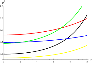
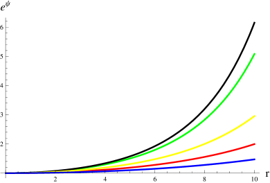
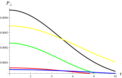
This section examines different physical features of the considered strange stars which are coupled with anisotropic configuration in scenario. We observe the graphical behavior of matter variables by using the masses and radii of each star candidate as shown in Table . We analyze the viability of metric potentials, energy density, radial and tangential components of pressure, anisotropy, energy bounds, compactness as well as redshift for the considered quark candidates and also investigate their stability, where the model parameter has been kept fixed. We are familiar with the fact that the compatibility of a solution guarantees the non-singular and monotonically increasing nature of metric components, having positive values throughout. Equation (21) shows that the metric coefficients depend only on Krori-Barua constants. By utilizing these constants for particular stars calculated in Table , the graphical behavior of both metric functions is analyzed in Figure which assures the physical consistency of the developed solution. It should be noted that the yellow color expresses 4U 1820-30 compact star, blue indicates Vela X-I, black represents SAX J 1808.4-3658, green signifies RXJ 1856-37 and red color shows Her X-I in all plots.
| Star Models | 4U 1820-30 | Vela X-I | SAX J 1808.4-3658 | RXJ 1856-37 | Her X-I |
| 2.25 | 1.77 | 1.435 | 0.9041 | 0.88 | |
| 10 | 12.08 | 7.07 | 6 | 7.7 | |
| 0.331 | 0.215 | 0.298 | 0.222 | 0.168 | |
| 0.000139001 | 0.000073158 | 0.000265408 | 0.000303665 | 0.000147867 |
| Star Models | 4U 1820-30 | Vela X-I | SAX J 1808.4-3658 | RXJ 1856-37 | Her X-I |
|---|---|---|---|---|---|
| 0.0108323 | 0.0038614 | 0.0181686 | 0.0162557 | 0.0069063 | |
| 0.0097711 | 0.0025930 | 0.0148019 | 0.0110467 | 0.0042674 | |
| -2.06034 | -0.94188 | -1.64803 | -0.98289 | -0.66249 |
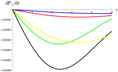
4.1 Inspection of Physical Parameters
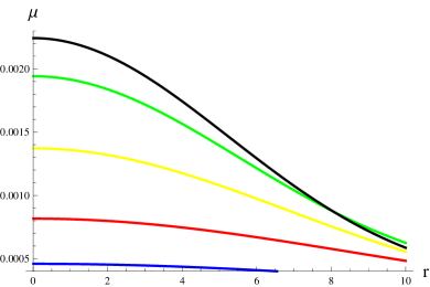
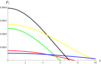
The composition of compact gravitational bodies indicates that the energy density and both pressure ingredients should be maximum inside the stellar structure. Figure exhibits the variation in these parameters with respect to each quark candidate for the model (8). These graphs clearly demonstrate that the energy density and pressure components gain their maximum values at the center () of anisotropic configured stars, resulting in the existence of extremely dense structures. Figure (b) also shows that the radial pressure inside the considered strange stars disappear at the boundary, while the energy density and tangential pressure decrease linearly with the rise in . The matter variables fulfill and as shown in Figure , thus they yield regular behavior. As a result, we observe from this graphical analysis that there must exist highly compact stars having anisotropic configuration in gravity.
 |
 |
| (a) | (b) |
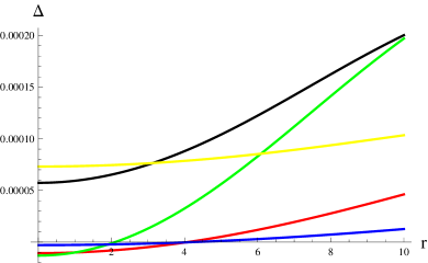
4.2 Effect of Anisotropic Pressure
We calculate the anisotropic factor in terms of Krori-Barua ansatz and bag constant by making use of Eqs.(23) and (24) as
| (33) |
 |
 |
| (a) | (b) |
 |
| (c) |
We use the observational data of various considered stars (shown in Table ) to analyze the behavior of anisotropy in their structural evolution. There occur an outward directed anisotropic pressure for the case when which yields . On the other hand, the condition (i.e., ) leads to the inward directed pressure. The effect of anisotropy on different stars is shown in Figure corresponding to the viable model of theory. It is noticed that remains positive throughout only for 4U 1820-30 and SAX J 1808.4-3658 stars which assures that there exists a repelling force which contributes to structural evolution of massive geometries, while this factor varies from negative to positive in the interior of remaining three candidates.
 |
 |
| (a) | (b) |
 |
| (c) |
 |
 |
| (a) | (b) |
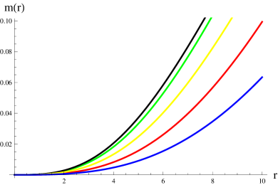
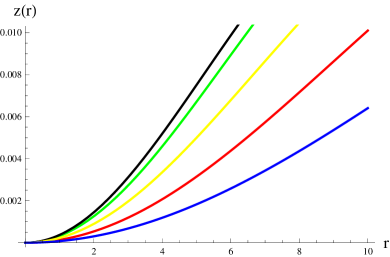
4.3 Mass, Compactness and Surface Redshift
For spherical structures, the mass can be defined as
| (34) |
where is given in Eq.(22). For our proposed model, we analyze the graphical behavior of the mass of considered stars by solving the above equation numerically along with an initial condition , as can be seen from Figure . We can characterize a celestial structure by its different physical features, among them one is the compactness which defines as the ratio of mass and radius. After employing the matching conditions between inner and outer spacetimes at , Buchdahl [64] found upper bound of . He disclosed that the system will remain stable for its value not to be greater than . There occur some reactions in the core of a massive body (having a strong gravitational force) due to which the electromagnetic radiations diffuse from that body. The redshift factor measures the increment in wavelength of those radiations. Mathematically, it is characterized as
| (35) |
This factor plays an influential role to study the particles existing in the inner geometry and its EoS. For perfect fluid distribution, Buchdahl found its value as , whereas Ivanov [65] studied anisotropic compact stars and observed its upper limit to be 5.211. Figure shows the plots for compactness as well as redshift for all quark candidates. It can be seen that the values of both factors are in their desired ranges.
 |
 |
| (a) | (b) |
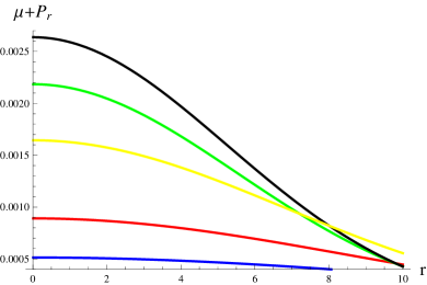
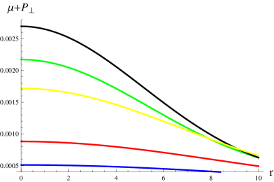
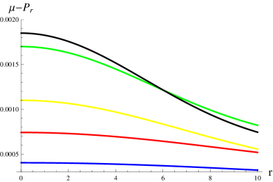
4.4 Energy Conditions
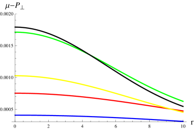
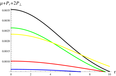
The existence of matter configuration in a stellar body can be demonstrated by some bounds, known as energy conditions which are of great importance in astrophysics. We can distinguish the usual or exotic matter existing inside the geometry by employing such conditions. They also help to investigate viability of the developed solutions in any gravitational theory. The physical parameters representing a particular geometry having ordinary matter must fulfill these conditions. The energy bounds for anisotropic configured star in gravity are
| (36) |
The plots of all the above conditions are shown in Figure . It is found that these conditions possess positive trend which assure the viability of the chosen model and the resulting solution. Thus there must exist normal matter in the interior of all quark candidates.
 |
 |
| (a) | (b) |
 |
 |
| (c) | (d) |
 |
| (e) |
4.5 Stability Analysis
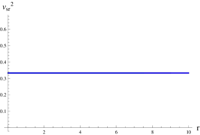
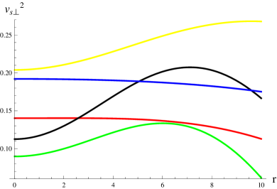
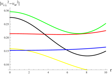
The stability of a compact star attains great significance in astrophysics to analyze physically feasible models. The massive bodies which show stable behavior against all the external fluctuations are more intriguing, thus this phenomenon has considerable interest in the study of their structural development. To analyze the stability of considered candidates in gravity, we employ two approaches, one of them is the cracking concept presented by Herrera [36] which is based on sound speed. The causality condition declares that the squared sound speed should lie within , i.e., throughout for stable structure. This becomes in the case of anisotropic matter as and , where represents the radial and shows tangential ingredients of sound speed. Thus the fulfilment of the inequality guarantees the stability of compact object. Figure indicates that all the considered candidates are stable for their respective calculated values of bag constant and .
 |
 |
| (a) | (b) |
 |
| (c) |
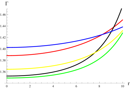
Secondly, the adiabatic index is considered as a powerful tool to analyze the stability of stellar geometry. This technique has been utilized to study the stable self-gravitating objects in which the adiabatic index should have its value greater than everywhere [66]. In this case, is characterized as
| (37) |
Figure demonstrates the physical behavior of for all candidates which fully agrees with the desired limit throughout the structure.
5 Conclusions
This paper discusses the effect of MIT bag constant () on physical attributes of five different strange anisotropic stars, namely 4U 1820-30, Vela X-I, SAX J 1808.4-3658, RXJ 1856-37 and Her X-I in theory of gravity. We analyze the influence of strong non-minimal coupling between matter and geometry in this theory (which appears due to the factor ) by adopting a linear model , where the coupling constant has been kept fixed as . We have formulated the field equations as well as TOV equation with the use of bag model EoS (17) and also calculated the values of corresponding to each star candidate (Table ). We have utilized the values of the metric potentials proposed by Krori-Barua involving three unknowns whose values have been evaluated in terms of masses and radii through matching conditions in this theory. The observational data of various star candidates has been used to calculate this triplet (Table ). We have found analytic solution of the modified field equations by taking two different equations of state relating energy density with pressure components. The graphical analysis of all quark candidates has been presented. It is found that the physical parameters attained their maximum (positive) values at the center (), while the behavior of anisotropy is increasing towards boundary.
The observed values of redshift and compactness are within their respective bounds. The energy conditions are fulfilled which confirm the existence of usual matter inside all the quark candidates as well as the viability of our developed solution. Two different techniques have been used to analyze the stability. We have determined that the potentially stable structure of these stars exist as the inequalities and hold throughout the system. The adiabatic index for all the considered stars has been visualized which also assures their stable structures. It is worthwhile to note that the quark star 4U 1820-30 shows more stable behavior towards the boundary in comparison with other four candidates (Figure ). It is concluded that the non-minimal matter-geometry interaction in theory may yield more appropriate results for compact structures as compared to [23, 24]. We have found that the chosen model (8) has viable behavior as the compact structures obtained with the help of MIT EoS (17) meet the needed requirements. Finally, we can retrieve all these results in GR for in functional form (8).
Appendix A
The value of adiabatic index in terms of Krori-Barua solution takes the form
The term in modified gravity becomes
References
- [1] S Nojiri and S D Odintsov, Phys. Rev. D 68, 123512 (2003)
- [2] G Cognola, E Elizalde, S Nojiri, S D Odintsov and S Zerbini, J. Cosmol. Astropart. Phys. 2005, 010 (2005)
- [3] Y S Song, W Hu and I Sawicki, Phys. Rev. D 75, 044004 (2007)
- [4] S Capozziello, M De Laurentis, S D Odintsov and A Stabile, Phys. Rev. D 83, 064004 (2011)
- [5] M Sharif and H R Kausar, J. Cosmol. Astropart. Phys. 2011, 022 (2011)
- [6] S Arapoğlu, C Deliduman and K Y Ekşi, J. Cosmol. Astropart. Phys. 2011, 020 (2011)
- [7] R Goswami, A M Nzioki, S D Maharaj and S G Ghosh, Phys. Rev. D 90, 084011 (2014)
- [8] M Sharif and Z Yousaf, Astropart. Phys. 56, 19 (2014)
- [9] A V Astashenok, S Capozziello and S D Odintsov, Phys. Rev. D 89, 103509 (2014)
- [10] O Bertolami, C G Boehmer, T Harko and F S N Lobo, Phys. Rev. D 75, 104016 (2007)
- [11] T Harko, F S N Lobo, S Nojiri and S D Odintsov, Phys. Rev. D 84, 024020 (2011)
- [12] M Sharif and M Zubair, J. Cosmol. Astropart. Phys. 2012, 028 (2012)
- [13] H Shabani and M Farhoudi, Phys. Rev. D 88, 044048 (2013)
- [14] P H R S Moraes, J D V Arbañil and M Malheiro, J. Cosmol. Astropart. Phys. 2016, 005 (2016)
- [15] M Sharif and A Siddiqa, Eur. Phys. J. Plus 132, 1 (2017)
- [16] A Das, S Ghosh, B K Guha, S Das, F Rahaman and S Ray, Phys. Rev. D 95, 124011 (2017)
- [17] Z Haghani, T Harko, F S N Lobo, H R Sepangi and S Shahidi, Phys. Rev. D 88, 044023 (2013)
- [18] M Sharif and M Zubair, J. High Energy Phys. 2013, 79 (2013)
- [19] M Sharif and M Zubair, J. Cosmol. Astropart. Phys. 2013, 042 (2013)
- [20] S D Odintsov and D Sáez-Gómez, Phys. Lett. B 725, 437 (2013)
- [21] I Ayuso, J B Jiménez and A De la Cruz-Dombriz, Phys. Rev. D 91, 104003 (2015)
- [22] E H Baffou, M J S Houndjo and J Tosssa, Astrophys. Space Sci. 361, 376 (2016)
- [23] M Sharif and A Waseem, Eur. Phys. J. Plus 131, 1 (2016)
- [24] M Sharif and A Waseem, Can. J. Phys. 94, 1024 (2016)
- [25] Z Yousaf, M Z Bhatti and T Naseer, Eur. Phys. J. Plus 135, 353 (2020)
- [26] Z Yousaf, M Z Bhatti and T Naseer, Phys. Dark Universe 28, 100535 (2020)
- [27] Z Yousaf, M Z Bhatti and T Naseer, Int. J. Mod. Phys. D 29, 2050061 (2020)
- [28] Z Yousaf, M Z Bhatti and T Naseer, Ann. Phys. 420, 168267 (2020)
- [29] Z Yousaf, M Z Bhatti, T Naseer and I Ahmad, Phys. Dark Universe 29, 100581 (2020)
- [30] Z Yousaf, M Y Khlopov, M Z Bhatti and T Naseer, Mon. Not. R. Astron. Soc. 495, 4334 (2020)
- [31] M Sharif and T Naseer, Chin. J. Phys. 73, 179 (2021)
- [32] T Naseer and M Sharif, Universe 8, 62 (2022)
- [33] E Witten, Phys. Rev. D 30, 272 (1984)
- [34] A R Bodmer, Phys. Rev. D 4, 1601 (1971)
- [35] I Bombaci, Phys. Rev. C 55, 1587 (1997)
- [36] L Herrera, Phys. Lett. A 165, 206 (1992)
- [37] L Herrera and N O Santos, Phys. Rep. 286, 53 (1997)
- [38] T Harko and M K Mak, Ann. Phys. 11, 3 (2002)
- [39] S K M Hossein, F Rahaman, J Naskar, M Kalam and S Ray, Int. J. Mod. Phys. D 21, 1250088 (2012)
- [40] M Kalam, F Rahaman, S Molla and S K M Hossein, Astrophys. Space Sci. 349, 865 (2014)
- [41] B C Paul and R Deb, Astrophys. Space Sci. 354, 421 (2014)
- [42] G H Bordbar and A R Peivand, Res. Astron. Astrophys. 11, 851 (2011)
- [43] P Haensel, J L Zdunik and R Schaefer, Astron. Astrophys. 160, 121 (1986)
- [44] K S Cheng, Z G Dai and T Lu, Int. J. Mod. Phys. D 7, 139 (1998)
- [45] P B Demorest, T Pennucci, S M Ransom, M S E Roberts and J W T Hessels, Nature 467, 1081 (2010)
- [46] F Rahaman, K Chakraborty, P K F Kuhfittig, G C Shit and M Rahman, Eur. Phys. J. C 74, 1 (2014)
- [47] P Bhar, Astrophys. Space Sci. 357, 1 (2015)
- [48] J D V Arbañil and M Malheiro, AIP Conf. Proc. 1693, 030007 (2015)
- [49] D Deb, S R Chowdhury, S Ray, F Rahaman and B K Guha, Ann. Phys. 387, 239 (2017)
- [50] D Deb, M Khlopov, F Rahaman, S Ray and B K Guha, Eur. Phys. J. C 78, 465 (2018)
- [51] M Sharif and A Waseem, Eur. Phys. J. C 78, 868 (2018)
- [52] M Sharif and A Waseem, Int. J. Mod. Phys. D 28, 1950033 (2019)
- [53] M Sharif and A Waseem, Chin. J. Phys. 63, 92 (2020)
- [54] M Sharif and A Majid, Eur. Phys. J. Plus 135, 1 (2020)
- [55] M Sharif and A Majid, Universe 6, 124 (2020)
- [56] M Sharif and A Majid, Astrophys. Space Sci. 366, 1 (2021)
- [57] N K Glendenning, Phys. Rev. D 46, 1274 (1992)
- [58] M Kalam, A A Usmani, F Rahaman, S M Hossein, I Karar and R Sharma, Int. J. Theor. Phys. 52, 3319 (2013)
- [59] J D V Arbañil and M Malheiro, J. Cosmol. Astropart. Phys. 2016, 012 (2016)
- [60] K D Krori and J Barua, J. Phys. A: Math. Gen. 8, 508 (1975)
- [61] K Lake, Phys. Rev. D 67, 104015 (2003)
- [62] M Dey, I Bombaci, J Dey, S Ray and B C Samanta, Phys. Lett. B 438, 123 (1998)
- [63] X D Li, I Bombaci, M Dey, J Dey and E P J Van Den Heuvel, Phys. Rev. Lett. 83, 3776 (1999)
- [64] H A Buchdahl, Phys. Rev. 116, 1027 (1959)
- [65] B V Ivanov, Phys. Rev. D 65, 104011 (2002)
- [66] H Heintzmann and W Hillebrandt, Astron. Astrophys. 38, 51 (1975)