Power Domination and Resolving Power Domination of Fractal Cubic Network
Abstract
In network theory, the domination parameter is vital in investigating several structural features of the networks, including connectedness, their tendency to form clusters, compactness, and symmetry. In this context, various domination parameters have been created using several properties to determine where machines should be placed to ensure that all the places are monitored. To ensure efficient and effective operation, a piece of equipment must monitor their network (power networks) to answer whenever there is a change in the demand and availability conditions. Consequently, phasor measurement units (PMUs) are utilised by numerous electrical companies to monitor their networks perpetually. Overseeing an electrical system which consists of minimum PMUs is the same as the vertex covering the problem of graph theory, in which a subset of a vertex set is a power dominating set (PDS) if it monitors generators, cables, and all other components, in the electrical system using a few guidelines. Hypercube is one of the versatile, most popular, adaptable, and convertible interconnection networks. Its appealing qualities led to the development of other hypercube variants. A fractal cubic network is a new variant of the hypercube that can be used as a best substitute in case faults occur in the hypercube, which was wrongly defined in [Eng. Sci. Technol. 18(1) (2015) 32-41]. Arulperumjothi et al. have recently corrected this definition and redefined this variant with the exact definition in [Appl. Math. Comput. 452 (2023) 128037]. This article determines the PDS of the fractal cubic network. Further, we investigate the resolving power dominating set (RPDS), which contrasts starkly with hypercubes, where resolving power domination is inherently challenging.
Keywords: fractal cubic network; hypercube variant; power domination; phase measuring units; resolving power domination
Mathematics Subject Classification (2020): 05C69 05C12
1 Introduction
The electrical nodes and connection wires constitute an electrical power network. Electric power corporation must continuously monitor their systems’ conditions. It is necessary to regulate the deployment of PMUs at precise position within the device.
Owing to the rising cost of PMUs, it is essential to engage as few as feasible while still tracking the entire system. This problem is introduced as a theoretical problem in [1], and coined it as a power domination problem after [2] evince its existence.
Let be a simple connected graph whose vertex set (electrical hubs) and edge set (connecting cables), respectively, is denoted by and . If the graph is clear from the context, we write and . Two vertices and of are adjacent if . Two adjacent vertices are called neighbors. For and for a vertex , the open -neighborhood of is denoted by and is defined as the collection of vertices that are at distance from . The closed -neighborhood of is , which is formally denoted by . When , the open -neighborhood of is called its open neighborhood and the closed -neighborhood of is called its closed neighborhood. For a set , its open neighborhood is the set , and its closed neighborhood is the set . The degree of a vertex in is the number of vertices adjacent to in , and is denoted by , and so . We let and . Also, we use to denote .
A set is a dominating set of if every vertex in is adjacent to at least one vertex in . A vertex in dominates itself and all its neighbors, and a set dominates a set in if every vertex in is dominated by at least one vertex in . Thus a dominating set of dominates every vertex in . The domination number of , denoted by , is the minimum cardinality of a dominating set in . We refer [3, 9, 4, 5, 6, 7, 8, 10, 11, 12] for a detailed study of domination and its variants.
If is observed or recursively observed by the following two rules with respect to a set of vertices in , then is called power dominating set, abbreviated PDS of .
-
1.
Domination:
-
2.
Propagation:
s.t.
In the domination step of PDS, all vertices in are monitored. In the event of the propagation phase of PDS, whenever a vertex is monitored, and is monitored, then the vertex is added to the set and is also monitored. An initial set in the first step is a PDS for if upon completion of the propagation phase the resulting set is the entire vertex set . The term is used to denote the minimum cardinality of a PDS in called the power domination number.
Investigation of PDS for arbitrary general graphs is NP-complete. It remains NP-complete for classes of graphs such as bipartite, chordal, and split graphs [1]. Numerous algorithms for fetching the PDS for a particular graph family were reported in [1, 14, 13]. This invariant is investigated for generalized Petersen family of graphs [15, 18, 16, 17], hypercubes [19], circular-arc graphs [20], block graphs [21], permutaion graphs [22], grids [23], planar and maximal planar graphs [24], Hanoi and Knödel graphs [25], Kautz and de Bruijn graphs [26], claw-free regular graphs [27] and octahedral structures [28]. Also, for graph operations like strong and tensor product [29], Cartesian product [15, 30], join and corona product [31], the PDS problem is examined. The lower bounds [33], upper bounds [34], and NG (Nordhaus-Gaddum) type results on PDS were discussed in [32]. An excellent survey on this topic can be seen in the book chapter by Dorbec [35].
The concept of a -power dominating set, abbreviated -PDS, was introduced in [16], where a -PDS is a traditional dominating set and a -PDS is the original power dominating set PDS. This parameter is investigated for certain interconnection networks [36], weighted trees [37], Sierpiński networks [38], block graphs [39], regular graphs [40]. Few more variation namely power dominating throttling [41] and infectious power domination [42] are recent and interesting problems.
The concept of metric dimension (MD) was primarily discussed in [43] and separately in [44]. It is equivalent to the least number of landmark vertices from which any two vertices can be differentiated using the distance parameter. The applications of this problem arise in various branches of science and technology.
The graph geodesic between two vertices and is the length (in terms of the number of edges) of the shortest path between and . The diameter of is the maximum length of a geodesic in . The maximum distance over all pairs of is called diameter.
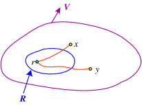
For a vertex , the code of with respect to the subset of is termed as a -vector
where is the geodesic from to for . The proper subset is a basis or resolving set for if any two distinct vertices of have nonidentical codes w.r.t . Equivalently, for any two distinct vertices , there exist a vertex such that . See Figure 1. The basis of with fewer cardinality is called the resolving number (also called the basis dimension) of and is denoted by . More on this topic and some of its recent works can be found in [45, 47, 46, 48].
2 Fractal Cubic Network: A New Hypercube Variant
Frequently, an interconnection networks with multiprocessors are essential to link an eloquent portion of dependably imitated processors (vertices). In lieu of shared memory, message transient is mostly used to afford complete transmission and synchronisation between processors for programmed execution. Owing to the availability of cost-effective, potent memory circuits and microprocessors, there has been a recent surge in fascination in implementing and designing multistage networks.
In parallel computing and supercomputers, interconnection networks, the development of CPUs, and routing algorithms are three primary research areas. The interconnection network, which connects millions of processors, is essential for the development of a supercomputer.
Multiple processors, each with their own cognitive connections (edges) and local sensing that enable data transfer between processors (vertices), compose an interconnection network. It can be represented as the previously defined graph in which two vertices and are directly connected by a communication connection. The attribute used to evaluate the productiveness of the networks are the bisection width, broadcasting time, fault-tolerance, degree, and diameter [50].
The hypercube is a common interconnection network design distinguished by its regularity, ease of transit, recursive structure, symmetry, and high connectedness. In recent years, hypercubes have been the subject of extensive research into their various properties [51].
There are many hypercube variations in the literature, including exchanged hypercube [52], folded hypercubes [53, 54], crossed cubes [55, 56], exchanged crossed cube [57], twisted cubes [58, 59], locally twisted cubes [60], shuffle cubes [61], spined cubes [62], Möbius cubes [63], and augmented cubes [64]. The hierarchical cubic network (HCN) [65, 66] and its folded version in [67] have also been ideas put forth based on a hierarchical framework employing the base hypercube as an introductory module.
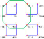
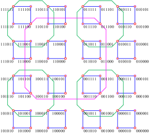
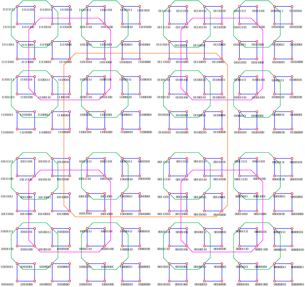
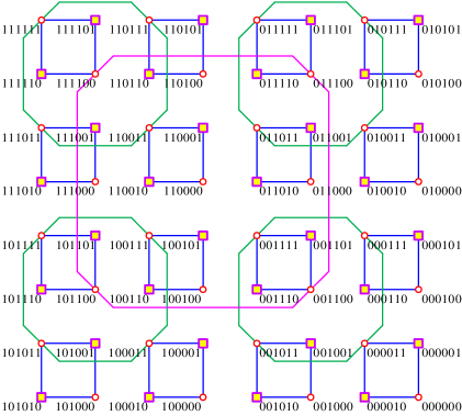
Despite the fact that numerous studies have been conducted on the variants of hypercube enumerated above, the problem resolving number has not been investigated for any of these variants except fractal cubic network. With this motivation, we investigate power domination and resolving power domination for the newly proposed hypercube variant fractal cubic network (FCN) [68]. Though the definition of this architecture is not clear in [68], we corrected this definition in [45]. We define as a cycle with four vertices , , , and . For , we define as follows:
An -dimensional FCN is defined as , , and can be constructed as follows
where
and
Figure 2(a)-(d), respectively, denotes the , , , and .
We denote as the collection of strings obtained by concatenating and each of the strings in . For , is constructed from four copies of with four additional edges connecting them.
3 Main Results
Before proceeding to the main arguments, we first present some preliminary lemma and results that are crucial for our investigation.
3.1 Twin Nodes
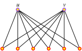
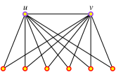
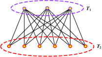
Two vertices are said to be non-adjacent twins (also called open twins in the literature) if and are adjacent twins (also called closed twins in the literature) if (see [69, 70]). The vertices and shown in Figure 3(a) are open twins, while the vertices and shown in Figure 3(b) are closed twins. Two vertices in are twins if they are open or closed twins in . A set is a open twin set or open twin class of , if every pair of vertices in are open twins in , while a set is a closed twin set or closed twin class of , if every pair of vertices in are closed twins in . The sets and shown in Figure 3(c) are examples of two open twin sets.
Arulperumjothi, Klavžar, and Prabhu [45] determined , where and .
Theorem 1.
[45] For , .

We proceed further with the following two key lemmas.
Lemma 2.
Let be a connected graph. If is a PDS of and is an open twin class of , then or .
Proof.
Let be a connected graph, and let be a PDS of and an open twin class of . We note that is an independent set and . Moreover every is adjacent to every . Thus, every path connecting a vertex in and a vertex in must contain a vertex in . We show that or . Suppose, to the contrary, that and . Let (possibly, which occurs is ), and so . Since is an independent set and since , no vertex in is adjacent to a vertex in . Thus, contains no vertex in , and so no vertex of is dominated in the initial domination step of PDS. As observed earlier, every path connecting a vertex in and a vertex in must contain a vertex in . Hence in order to observe the vertices in we must first observe a vertex in either by domination or by propagation from the vertices that do not belong to the set . However, every vertex in is adjacent to all vertices of . Thus the vertices of cannot be propagated as every vertex of has vertices as neighbors. This contradicts the supposition that is a PDS of . ∎
Lemma 3.
If is a connected graph with vertex disjoint twin classes such that for every , then .
Proof.
Let be a PDS of . By Lemma 2, or for all . Thus since , we note that if , then . Hence at least one of or holds for all , implying that for all . By supposition, the twin classes are vertex disjoint. Further, the sets and are vertex disjoint for every . From this we infer that
Since in arbitrary PDS of , we infer that . ∎
We are now in a position to prove the following result.
Theorem 4.
For , .
Proof.
Let . From the definition of , we note that , where . That is, is an open twin set in . The and its twin sets are marked in Figure 4. Hence, contains twin sets, each containing exactly two vertices. Therefore by Lemma 3, .
To show that , let
where the union is taken over all . We note that . Let . We claim that the set is a power dominating set of . For this, we have to prove that every vertex of is monitored by the vertices of either by domination or by propagation. We note that , where as before . Hence, . Thus, all vertices in are monitored by the vertices of by domination. We note further that is an independent set and that . Also, each vertex is of degree in and is adjacent to vertex , where . Moreover, the vertices in are pairwise at distance at least apart, and so no two vertices in have a common neighbor that belongs to . Thus every dominated vertex in has all its neighbors dominated, except for exactly one vertex in . Thus, each dominated vertex in propagates to its unique neighbor in . Thus, each vertex is propagated by either or . Hence, , that is, is a power dominating set of , implying that . As observed earlier, . Consequently, . ∎
4 Resolving Power Domination of FCN
This section recalls the definition of a resolving-power dominating set and its minimum cardinality. A subset is both resolving and power-dominating. The subset of is called a resolving-power dominating set, and its minimum cardinality is the resolving power domination number and is notated by . The first paper on this notion was introduced in [71].
Theorem 5.
[71] For any simple connected graph , .
Since then, we are not aware of further research on this problem. Prabhu et al. recently investigated this parameter for probabilistic neural networks (PNN) in [48]. As a consequence of our main results in this paper, we determine the resolving power domination number of a fractal cubic network.
Theorem 6.
For , .
5 Conclusion
Multistage interconnection networks are essential to parallel computing because their performance on a large scale is determined by their connectivity. Communication efficacy is a key prosecution indicator in parallel computing. The diameter of a network’s interconnections is an essential metric of transmission efficiency. Hypercube is prevalent in all architecture owing to its advantageous properties. There are numerous prospective variants of this network that can be created by modifying certain links. This variant of hypercube is one such variant. In the present investigation, we concentrate on power domination and resolving-power domination for this new invariant in the most optimal manner. In this paper, we completely determine these parameters for fractal cubic networks.
Compliance with ethical standards
Conflict of interest: The authors declare that there is no conflict of interest regarding the publication of this paper.
Data Availability Statement: No Data associated with the manuscript.
References
- [1] T.W. Haynes, S.M. Hedetniemi, S.T. Hedetniemi, M.A. Henning, Domination in graphs applied to electric power networks, SIAM Journal on Discrete Mathematics 15(4) 519–529.
- [2] T.L. Baldwin, L. Mili, M.B. Boisen, R. Adapa, Power system observability with minimal phasor measurement placement, IEEE Transactions on Power systems 8(2) (1993) 707–715.
- [3] D. Chalupa, An order-based algorithm for minimum dominating set with application in graph mining, Information Sciences 426 (2018) 101–116.
- [4] W. Chen, Z. Lu, W. Wu, Dominating problems in swapped networks, Information Sciences 269 (2014) 286–299.
- [5] C. Pang, R. Zhang, Q. Zhang, J. Wang, Dominating sets in directed graphs, Information Sciences 180(19) (2010) 3647–3652.
- [6] W.C.K. Yen, The bottleneck independent domination on the classes of bipartite graphs and block graphs, Information Sciences 157 (2003) 199–215.
- [7] Y.T. Tsai, Y.L. Lin, F.R. Hsu, Efficient algorithms for the minimum connected domination on trapezoid graphs, Information Sciences 177(12) (2007) 2405–2417.
- [8] L. Wu, E. Shan, Z. Liu, On the -tuple domination of generalized de Brujin and Kautz digraphs, Information Sciences 180(22) (2010) 4430–4435.
- [9] Z. Shao, M. Liang, C. Yin, X. Xu, P. Pavlič, J. Žerovnik, On rainbow domination numbers of graphs, Information Sciences 254 (2014) 225–234.
- [10] T. W. Haynes, S. T. Hedetniemi, and M. A. Henning (eds), Topics in Domination in Graphs. Series: Developments in Mathematics, Vol. 64, Springer, Cham, 2020. viii + 545 pp.
- [11] T. W. Haynes, S. T. Hedetniemi, and M. A. Henning (eds), Structures of Domination in Graphs. Series: Developments in Mathematics, Vol. 66, Springer, Cham, 2021. viii + 536 pp.
- [12] T. W. Haynes, S. T. Hedetniemi, and M. A. Henning, Domination in Graphs: Core Concepts. Series: Springer Monographs in Mathematics, Springer, Cham, 2023. xx + 644 pp.
- [13] A. Aazami, K. Stilp, Approximation algorithms and hardness for domination with propagation, SIAM Journal on Discrete Mathematics 23(3) (2009) 1382–1399.
- [14] J. Guo, R. Niedermeier, D. Raible, Improved algorithms and complexity results for power domination in graphs, Algorithmica 52 (2008) 177–202.
- [15] R. Barrera, D. Ferrero, Power domination in cylinders, tori, and generalized Petersen graphs, Networks 58(1) (2011) 43–49.
- [16] G.J. Chang, P. Dorbec, M. Montassier, A. Raspaud, Generalized power domination of graphs, Discrete Applied Mathematics 160(12) (2012) 1691–1698.
- [17] M. Zhao, E. Shan, L. Kang, Power domination in the generalized Petersen graphs, Discussiones Mathematicae Graph Theory 40(3) (2020) 695–712.
- [18] G. Xu, L. Kang, On the power domination number of the generalized Petersen graphs, Journal of Combinatorial Optimization 22 (2011) 282–291.
- [19] N. Dean, A. Ilic, I. Ramirez, J. Shen, K. Tian, On the power dominating sets of hypercubes, In 2011 14th IEEE International Conference on Computational Science and Engineering (2011) pp. 488–491.
- [20] C.S. Liao, D.T. Lee, Power domination in circular-arc graphs, Algorithmica 65(2) (2013) 443–466.
- [21] G. Xu, L. Kang, E. Shan, M. Zhao, Power domination in block graphs, Theoretical Computer Science, 359(1-3) (2006) 299–305.
- [22] S. Wilson, Power domination on permutation graphs, Discrete Applied Mathematics 262 (2019) 169–178.
- [23] M. Dorfling, M.A. Henning, A note on power domination in grid graphs, Discrete Applied Mathematics 154(6) (2006) 1023–1027.
- [24] P. Dorbec, A. González, C. Pennarun, Power domination in maximal planar graphs, Discrete Mathematics & Theoretical Computer Science 21(4) (2019) 1–24.
- [25] S. Varghese, A. Vijayakumar, A.M. Hinz, Power domination in Knödel graphs and Hanoi graphs, Discussiones Mathematicae Graph Theory 38(1) (2018) 63–74.
- [26] J. Kuo, W.L. Wu, Power domination in generalized undirected de Bruijn graphs and Kautz graphs, Discrete Mathematics, Algorithms and Applications 7(1) (2015) 1550003.
- [27] C. Lu, R. Mao, B. Wang, Power domination in regular claw-free graphs, Discrete Applied Mathematics 284 (2020) 401–415.
- [28] S. Prabhu, S. Deepa, R.M. Elavarasan, E. Hossain, Optimal PMU placement problem in octahedral networks, RAIRO-Operations Research 56(5) (2022) 3449–3459.
- [29] P. Dorbec, M. Mollard, S. Klavžar, S. Špacapan, Power domination in product graphs, SIAM Journal on Discrete Mathematics 22(2) (2008) 554–567.
- [30] K.M. Koh, K.W. Soh, On the power domination number of the Cartesian product of graphs, AKCE International Journal of Graphs and Combinatorics 16(3) (2019) 253–257.
- [31] I. Yuliana, I.H, Agustin, D.A.R. Wardani, On the power domination number of corona product and join graphs, Journal of Physics: Conference Series 1211(1) (2019) 012020.
- [32] K.F. Benson, D. Ferrero, M. Flagg, V. Furst, L. Hogben, V. Vasilevska, Nordhaus–Gaddum problems for power domination, Discrete Applied Mathematics 251 (2018) 103–113.
- [33] D. Ferrero, L. Hogben, F.H. Kenter, M. Young, Note on power propagation time and lower bounds for the power domination number, Journal of Combinatorial Optimization 34 (2017) 736–741.
- [34] M. Zhao, L. Kang, G.J. Chang, Power domination in graphs, Discrete Mathematics 306(15) (2006) 1812–1816.
- [35] P. Dorbec, Power domination in graphs. Topics in Domination in Graphs, 521–545. Series: Developments in Mathematics, Vol. 64, Springer, Cham, 2020.
- [36] R.S. Rajan, S Arulanand, S Prabhu, I Rajasingh, 2-power domination number for Knödel graphs and its application in communication networks, RAIRO-Operations Research 57(6) (2023) 3157–3168.
- [37] C. Cheng, C. Lu, Y. Zhou, The -power domination problem in weighted trees, Theoretical Computer Science 809(2) (2020) 231–238.
- [38] P. Dorbec, S. Klavžar, Generalized power domination: propagation radius and Sierpiński graphs, Acta Applicandae Mathematicae 134 (2014) 75–86.
- [39] C. Wang, L. Chen, C. Lu, -Power domination in block graphs, Journal of Combinatorial Optimization 31(2) (2016) 865–873.
- [40] P. Dorbec, M.A. Henning, C. Löwenstein, M. Montassier, A. Raspaud, Generalized power domination in regular graphs, SIAM Journal on Discrete Mathematics 27(3) (2013) 1559–1574.
- [41] B. Brimkov, J. Carlson, I.V. Hicks, R. Patel, L. Smith, Power domination throttling, Theoretical Computer Science 795 (2019) 142–153.
- [42] B. Bjorkman, Infectious power domination of hypergraphs, Discrete Mathematics 343(3) (2020) 111724.
- [43] P.J. Slater, Leaves of trees, Congressus Numerantium 14 (1975) 549–559.
- [44] F. Harary, R.A. Melter, On the metric dimension of a graph, Ars Combinatoria 2 (1976) 191–195.
- [45] M. Arulperumjothi, S. Klavžar, S. Prabhu, Redefining fractal cubic networks and determining their metric dimension and fault-tolerant metric dimension, Applied Mathematics and Computation 452 (2023) 128037.
- [46] S. Prabhu, V. Manimozhi, M. Arulperumjothi, S. Klavžar, Twin vertices in fault-tolerant metric sets and fault-tolerant metric dimension of multistage interconnection networks, Applied Mathematics and Computation 420 (2022) 126897.
- [47] S. Prabhu, D.S.R. Jeba, M. Arulperumjothi, S. Klavžar, Metric dimension of irregular convex triangular networks, AKCE International Journal of Graphs and Combinatorics https://doi.org/10.1080/09728600.2023.2280799 (2023).
- [48] S. Prabhu, S. Deepa, M. Arulperumjothi, L. Susilowati, J.-B. Liu, Resolving-power domination number of probabilistic neural networks, Journal of Intelligent & Fuzzy Systems 43(5) (2022) 6253–6263.
- [49] S. Prabhu, T. Flora, M. Arulperumjothi, On independent resolving number of TiO nanotubes, Journal of Intelligent & Fuzzy Systems 35(6) (2018) 6421–6425.
- [50] S.B. Akers, B. Krishnamurthy, A group-theoretic model for symmetric interconnection networks, IEEE Transactions on Computers 38(4) (1989) 555–566.
- [51] F. Harary, J.P. Hayes, H.J. Wu, A survey of the theory of hypercube graphs, Computers and Mathematics with Applications 15(4) (1988) 277–289.
- [52] P.K. Loh, W.J. Hsu, Y. Pan, The exchanged hypercube, IEEE Transactions on Parallel and Distributed Systems 16(9) (2005) 866–874.
- [53] A. El-Amawy, S. Latifi, Properties and performance of folded hypercubes, IEEE Transactions on Parallel and Distributed Systems 2(1) (1991) 31–42.
- [54] Q. Zhu, S.Y. Liu, M. Xu, On conditional diagnosability of the folded hypercubes, Information Sciences 178(4) (2008) 1069–1077.
- [55] K. Efe, The crossed cube architecture for parallel computation, IEEE Transactions on Parallel & Distributed Systems 3(5) (1992) 513–524.
- [56] J. Fan, X. Jia, Embedding meshes into crossed cubes, Information Sciences 177(15) (2007) 3151–3160.
- [57] K. Li, Y. Mu, K. Li, G. Min, Exchanged crossed cube: a novel interconnection network for parallel computation, IEEE Transactions on Parallel and Distributed Systems 24(11) (2013) 2211–2219.
- [58] S. Abraham, K. Padmanabhan, The twisted cube topology for multiprocessors: A study in network asymmetry, Journal of Parallel and Distributed Computing 13(1) (1991) 104–110.
- [59] C.P. Chang, J.N. Wang, L.H. Hsu, Topological properties of twisted cube, Information Sciences 113(1-2) (1999) 147–167.
- [60] X. Yang, D.J. Evans, G.M. Megson, The locally twisted cubes, International Journal of Computer Mathematics 82(4) (2005) 401–413.
- [61] T.K. Li, J.J. Tan, L.H. Hsu, T.Y. Sung, The shuffle-cubes and their generalization, Information Processing Letters 77(1) (2001) 35–41.
- [62] W. Zhou, J. Fan, X. Jia, S. Zhang, The spined cube: a new hypercube variant with smaller diameter, Information Processing Letters 111(12) (2011) 561–567.
- [63] P. Cull, S.M. Larson, The Mobius cubes, IEEE Transactions on Computers 44(5) (1995) 647–659.
- [64] S.A. Choudum, V. Sunitha, Augmented cubes, Networks: An International Journal 40(2) (2002) 71–84.
- [65] K. Ghose, K.R. Desai, Hierarchical cubic networks, IEEE Transactions on Parallel and Distributed Systems 6(4) (1995) 427–435.
- [66] S.K. Yun, K.H. Park, Comments on hierarchical cubic networks, IEEE Transactions on Parallel and Distributed Systems 9(4) (1998) 410–414.
- [67] D.R. Duh, G.H. Chen, J.F. Fang, Algorithms and properties of a new two-level network with folded hypercubes as basic modules, IEEE Transactions on Parallel and Distributed Systems 6(7) (1995) 714–723.
- [68] A. Karci, B. Selçuk, A new hypercube variant: fractal cubic network graph, Engineering Science and Technology: An International Journal 18(1) (2015) 32–41.
- [69] G.A. Barragán-Ramírez, A. Estrada-Moreno, Y. Ramírez-Cruz, J.A. Rodríguez-Velázquez, The local metric dimension of the lexicographic product of graphs, Bulletin of the Malaysian Mathematical Sciences Society 42(5) (2019) 2481–2496.
- [70] M.S. Lin, Simple linear-time algorithms for counting independent sets in distance-hereditary graphs, Discrete Applied Mathematics 239 (2018) 144–153.
- [71] S. Stephen, B. Rajan, C. Grigorious, A. William, Resolving-power dominating sets, Applied Mathematics and Computation 256 (2015) 778–785.