Enhancing Accuracy and Parameter-Efficiency of Neural Representations for Network Parameterization

Abstract

In this work, we investigate the fundamental trade-off regarding accuracy and parameter efficiency in the parameterization of neural network weights using predictor networks. We present a surprising finding that, when recovering the original model accuracy is the sole objective, it can be achieved effectively through the weight reconstruction objective alone. Additionally, we explore the underlying factors for improving weight reconstruction under parameter-efficiency constraints, and propose a novel training scheme that decouples the reconstruction objective from auxiliary objectives such as knowledge distillation that leads to significant improvements compared to state-of-the-art approaches. Finally, these results pave way for more practical scenarios, where one needs to achieve improvements on both model accuracy and predictor network parameter-efficiency simultaneously.

1 Introduction

Recently, neural network weight space exploration and manipulation have gained an increase in popularity as alternative avenues for traditional model training and fine-tuning. Examples of these methods range from weight manipulation strategies such as weight merging to improve model performance without fine-tuning (Matena and Raffel, 2022) to weight generation approaches that directly predict network parameters (Ashkenazi et al., 2022; Soro et al., 2024). One of these approaches uses implicit neural representations (INRs) to directly represent the weights of a pre-trained convolutional neural network (CNN), where the coordinates of the kernel or layer indices in the INR are mapped to the corresponding weights in the CNN (Ashkenazi et al., 2022). Despite the interesting formulation of the problem, the approach provides limited practical benefits, as the reconstructed weights invariably exhibit worse performance compared to the original model.

In this work, we are exploring the various trade-offs between predictor networks and reconstructed models as well as the effects of different training objectives and their interactions for network weight prediction tasks (Ashkenazi et al., 2022; Soro et al., 2024; Knyazev et al., 2023). We demonstrate that better-performing models can be obtained through a weight reconstruction-only objective and these improvements can be compounded over multiple repetitions. By iterating over the reconstruction process multiple times through repeatedly reconstructing the previously reconstructed weights, we establish an "inception"-like setup with nested improvements in each prediction round. Furthermore, we discovered that using multi-objective loss functions during the reconstruction process can lead to contradictory training signals, resulting in limited performance gains. Therefore, we propose a new training scheme that decouples the learning objectives into two phases: a reconstruction phase and a distillation phase, ensuring that each learning objective has the desired impact. Remarkably, our approach results in significant improvements compared to the selected state-of-the-art baseline while improving compression efficiency. Moreover, the proposed separation provides greater flexibility in the distillation step by allowing the use of powerful networks to be involved during the weight refinement. All these improvements and insights led to several usage scenarios that were not possible or practical before, for example, obtaining a better-performing model through a predictor network that is much smaller than the original network, or iterative improving a given model through the reconstruction process. The proposed approach provides a unique, even surprising, perspective for achieving model performance improvement that is different from existing weight manipulation approaches such as stochastic weight averaging (Guo et al., 2023a; Izmailov et al., 2018). We also achieve storage compression via the predictor network which is orthogonal and composable with existing model pruning (Lee et al., 2019; Liu et al., 2018; Gao et al., 2021; Wang et al., 2021; He and Xiao, 2023) and knowledge distillation approaches (Chen et al., 2020; Gou et al., 2021; Chen et al., 2017; Beyer et al., 2022).

2 Predicting Model Weights using Neural Representations

There is a growing interest in predicting the weights of pre-trained models not only to enhance the memory efficiency of model storage but also to improve the throughput of model inference. Existing solutions range from building high-fidelity auxiliary models (Knyazev et al., 2023) to learning parameter-efficient approximators (Guo et al., 2023b). However, in this paper, we focus on neural representations learning based on their flexibility and potential for producing effective, yet parameter-efficient, approximations for deep networks. The NeRN framework (Ashkenazi et al., 2022), introduced by Ashkenazi et al. first explored the idea of training INRs and demonstrated its utility in compressing CNNs. At its core, NeRN uses a 5-layer multilayer perceptron (MLP) $G_{\phi}$ with fixed hidden layer size to learn a mapping from an input tuple $($layer $\ell,$ filter $f,$ channel $c)$ to the corresponding $k\times k$ kernel in the original CNN model $F_{\theta}$. Note that the output size of the MLP also remains fixed at the largest kernel size and smaller kernels in the CNN are sampled from the middle while fully-connected or normalization layers are excluded based on their comparatively negligible parameter size. By utilizing positional encodings, e.g., SIREN (Sitzmann et al., 2020), the input coordinates are projected into a higher dimensional space, allowing NeRN to learn higher frequency functions and improve the approximation capabilities of the predictor. Since there is no inherent smoothness in the ordering of filters in a CNN, permutation strategies are introduced to rearrange filters in the original model based on similarity, ensuring stable training of NeRN.

The central component of NeRN training is the reconstruction loss aimed at quantifying the disparity between the original network weights and those recovered using the predictor. Regardless of the capacity of $G_{\phi}$, one might expect that the reconstruction loss should reliably converge to a meaningful approximation. However, in practice, it has been found that NeRN is prone to training instabilities when the auxiliary model is smaller than the original network. To mitigate these issues, the authors introduced additional loss terms inspired by existing knowledge distillation methods. However, it is important to note that while the reconstruction loss does not require access to training data, the distillation loss does, making it impractical for scenarios where access to the training data is not available. The overall objective function for NeRN can be expressed as

$$\mathcal{L}_{objective}=\mathcal{L}_{recon}+\alpha\mathcal{L}_{KD}+\beta\mathcal{L}_{FMD},\text{with}$$ (1)

$$\mathcal{L}_{recon}=\frac{1}{|\mathbf{W}|}\|\mathbf{W}-\mathbf{\hat{W}}\|_{2},\phantom{a}\mathcal{L}_{FMD}=\frac{1}{|\mathcal{B}|}\sum_{i\in\mathcal{B}}\sum_{l}\|\mathbf{a}^{l}_{i}-\mathbf{\hat{a}}^{l}_{i}\|_{2},\phantom{a}\mathcal{L}_{KD}=\frac{1}{|\mathcal{B}|}\sum_{i\in\mathcal{B}}KL(\mathbf{a}^{\text{out}}_{i},\mathbf{\hat{a}}^{\text{out}}_{i}),$$

where $\mathbf{W}=[\mathbf{w}^{0},\mathbf{w}^{1},...,\mathbf{w}^{L}]$, represents a list of convolutional weight vectors for layer $\ell$ in the original network, and $\hat{\mathbf{W}}$ denotes the corresponding weights of the reconstructed weights. The terms $\mathbf{a}^{\ell}_{i}$ and $\hat{\mathbf{a}}^{\ell}_{i}$ denote the ${L}_{2}$ normalized feature maps generated from the $i$-th sample in the minibatch $\mathcal{B}$ at layer $\ell$ for the original and reconstructed networks respectively. Additionally, the logit distillation loss $\mathcal{L}_{KD}$ employs the Kullback-Leibler divergence to compare the output logits $\mathbf{a}^{\text{out}}_{i}$ and $\hat{\mathbf{a}}^{\text{out}}_{i}$ from the original and reconstructed networks for each sample $i$ in the minibatch $\mathcal{B}$.

3 Proposed Approach

In this section, we take a closer look at learning neural representations for pre-trained neural networks. Specifically, we explore the role of different training objectives in realizing an effective parameterization. Based on our findings, we propose a new training scheme that circumvents the undesirable trade-off between accuracy and model compression rate, and simultaneously improve on both aspects.

3.1 Is the Reconstruction Objective All You Need?

A well-known limitation of existing approaches used for weight prediction is that they trade off accuracy to achieve parameter efficiency. This non-trivial compromise in model performance can be a critical bottleneck for practical applications. While existing approaches attempt to recover the lost performance through the use of additional objectives, e.g., distillation as in NeRN, they lead to increased reconstruction errors, albeit providing improvements in the accuracy. As this seems counter-intuitive, it naturally raises the question: what is the relation between reconstruction error and expected model performance?

If we assume that reconstruction error, e.g., mean-squared error (MSE), is indeed an indication for performance, a straightforward strategy to improve performance would be to increase the capacity of the predictor network, allowing it to overfit to the original model weights. To this end,

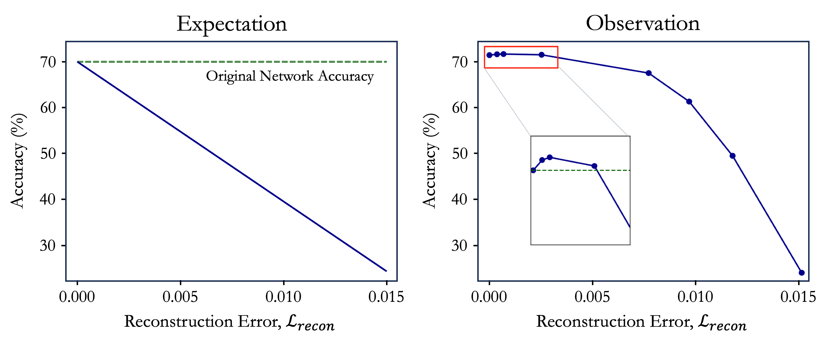
Figure 1: While one expects that the reconstruction error must approach zero to recover the true performance (left), we are able to find networks with non-zero (yet low) errors that not only match the true performance but even surpass it (right).

we first empirically analyze how well we can recover the original network’s performance, as we continually reduce the reconstruction error by increasing the predictor network capacity. Note, in this analysis, we are not concerned about parameter-efficiency, and the neural representations are trained solely based on reconstruction error. As shown in Figure 1 (left), one might expect that the parameterization should recover the performance of the original network as the reconstruction error approaches zero. However, by using only the reconstruction loss and increasing the predictor network capacity, we empirically find weight parameterizations with non-zero reconstruction errors that not only recover the true performance, but even surpass it (Figure 1 (right)).

How does reconstruction-only objective lead to better networks? A well-known property of the MSE

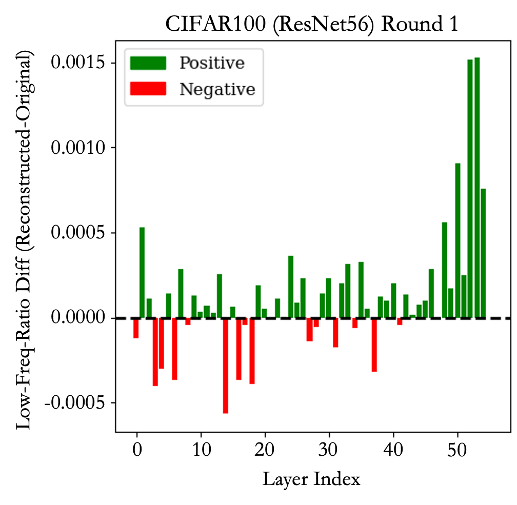
Figure 2: Measuring the dominance of low-frequency components in original and recovered networks.

loss is that it tends to have a smoothing effect on the reconstructed weights (Domingos, 2012). To quantify this, we compare the weights of the reconstructed network (based on neural representations learned using only the reconstruction objective) with those of the original network, in terms of changes in the ratio of low-frequency components of their weight matrices measured as follows: Let $\mathbf{M}$ be the weight matrix of a given layer, shaped as $\mathbf{M}\in\mathbb{R}^{n\times m}$. Using singular value decomposition (SVD) on this matrix, we obtain $\mathbf{M}=\mathbf{U}\mathbf{\Sigma}\mathbf{V}^{T}$ where $\mathbf{\Sigma}\in\mathbb{R}^{n\times m}$ is a diagonal matrix with singular values $\mathbf{s}=\left[\sigma_{1},\sigma_{2},\ldots,\sigma_{k}\right]$ on the diagonal and $k=\min(n,m)$. The $S_{ratio}$ is then calculated as $S_{ratio}=\sum_{i=1}^{\lfloor k/2\rfloor}\sigma_{i}^{2}/\sum_{i=1}^{k}\sigma_{i}^{2}$. This ratio measures the proportion of the total variance (energy) of the matrix $\mathbf{M}$ that is captured by the first half of the singular values. A higher ratio indicates that the lower frequency components are more dominant. As illustrated in Figure 2, we show a per-layer difference of $S_{ratio}$ between the reconstructed and original weights.

Upon close inspection, a clear trend emerges, where we find that the reconstructed weights correspond to more dominant low-frequency components compared to the original, particularly in the later layers, i.e., this smoothing leads to implicit rank reduction. Interestingly, this observation corroborates with the recent finding that rank reduction can help improve the behavior of even large scale models (Sharma et al., 2023).

Building upon our hypothesis about the effect of smoothing induced by the reconstruction objective, we ask the question: can multiple rounds of progressive, neural representation learning further improve the performance of the reconstructed network? To this end, we extend our previous experiment by training multiple generations of network parameterizations, wherein the first round predictor network attempts to reconstruct the original network, the second round predictor attempts to recover the reconstructed network from round 1, and so on.

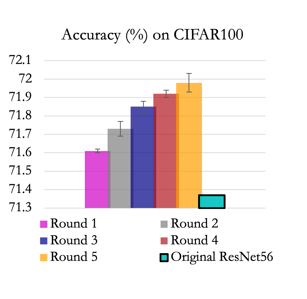
Figure 3: Evaluation of the reconstruction performance for each round of reconstruction.

Such a process resembles an "inception"-like setup where the new predictor is built on top of the previously reconstructed weights. We find that, this simple procedure leads to further improvements over the original network’s performance, albeit producing relatively higher reconstruction errors due to smoothing. As shown in Figure 3, this progressive training produces monotonic improvements in the accuracy, and in all cases superior to the original network’s performance. While this observation holds for all architectures and datasets, once weights are sufficiently smoothed, we do not witness further improvements by using additional rounds of training (performance does not drop either). Given the additional complexity in training multiple neural representations, in practice, even $1$ or $2$ rounds of progressive training is beneficial.

3.2 Distillation Improves Compression, But Only with Loss Decoupling

So far, we inspected the behavior of the reconstruction loss, and demonstrated its surprising efficacy in enhancing model performance. Despite the observed performance improvement, we did not take parameter-efficiency into account for our analysis. However, in practice, an important motivation for using weight prediction networks is to achieve signification reduction in memory requirements for model storage, while not trading-off the performance unreasonably. While neural representations were originally leveraged with such a compression objective (Ashkenazi et al., 2022), their accuracy trade-off makes them a less preferred choice over other model compression (or reduction) strategies in practice. In this section, we show how the compression capability of neural representations can be enhanced. To this end, we take a closer look at the widely adopted distillation objective and how it interacts with the reconstruction loss. By doing so, we address the critical need to strike a balance between model complexity and efficiency, paving the way for more practical and resource-efficient neural networks.

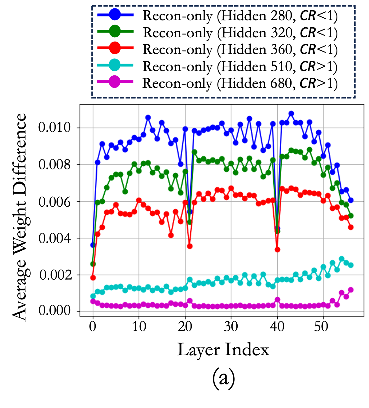
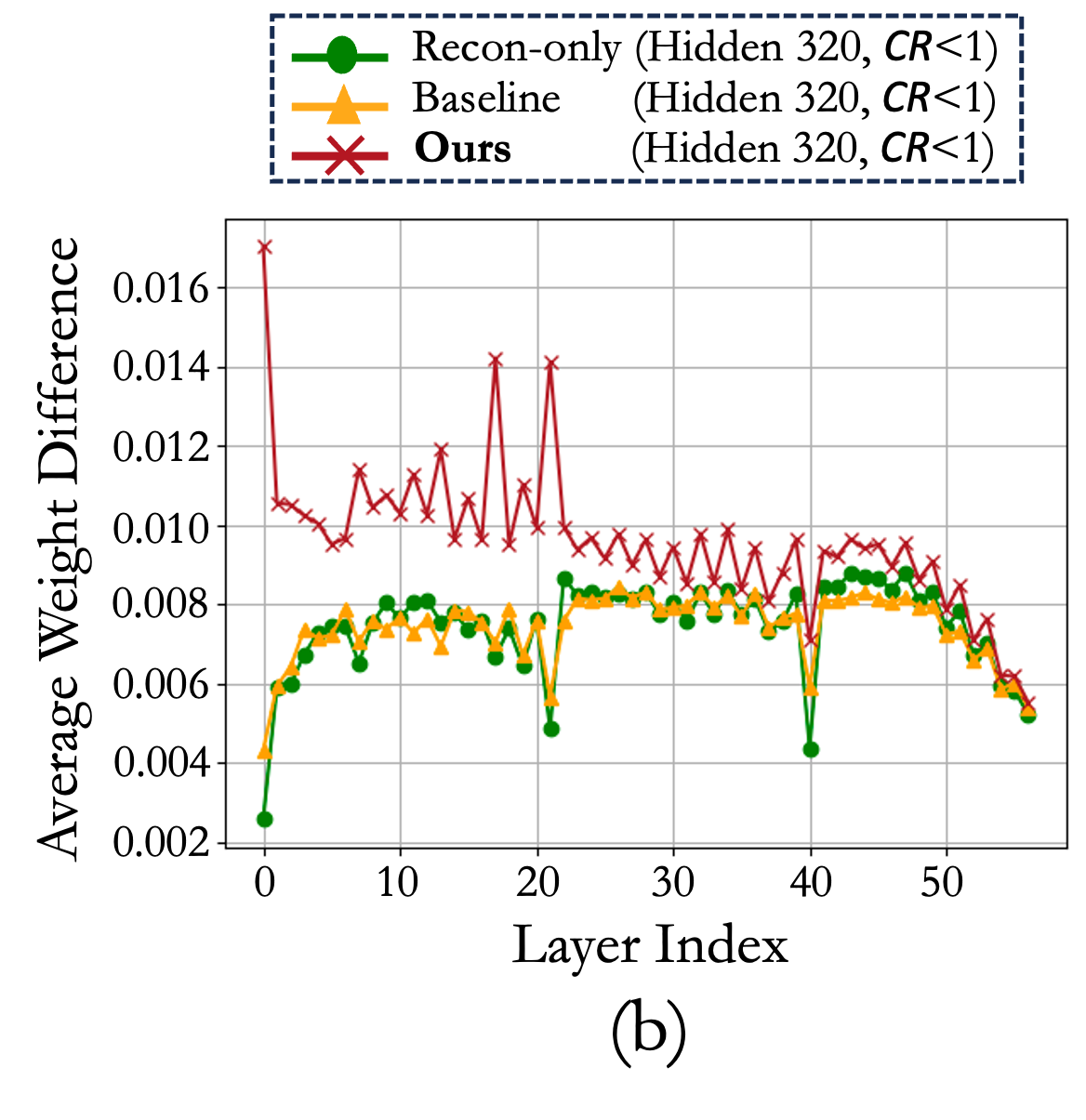
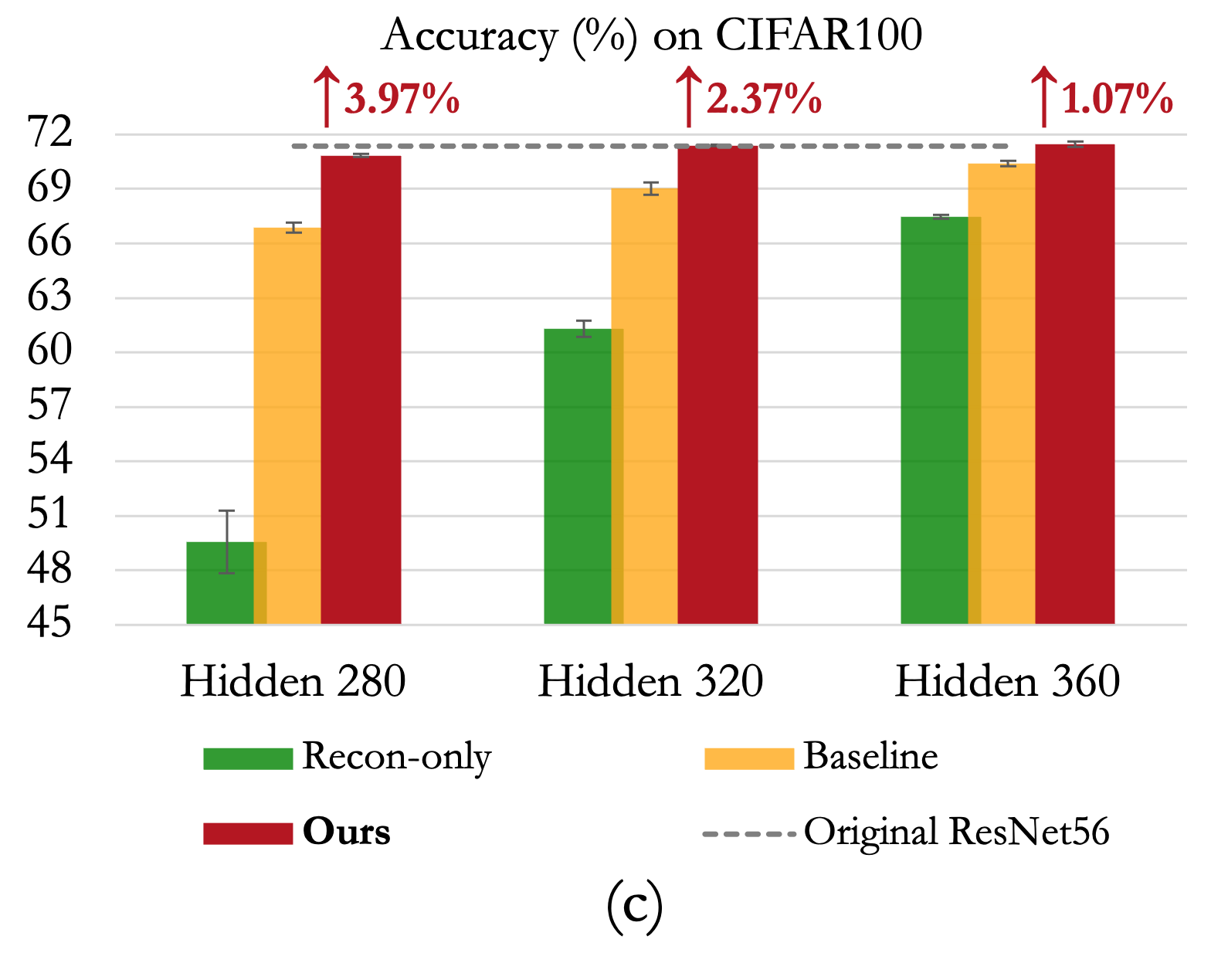
Figure 4: (a) Average weight difference between predicted weights by Recon-only and original weights with varying hidden sizes. (b) Comparison among Recon-only, baseline, and ours. (c) Evaluation of the reconstruction performance for each method. $\uparrow$ represents our performance improvement over the baseline.

To begin with, we analyze the layer-wise weight differences between the reconstructed and original networks at varying predictor network sizes (Figure 4(a)). Note, we use the term “CR” to denote the compression ratio, computed as the ratio of the learnable size of the predictor $S(P)$ to that of the original network $S(O)$. For instance, if the predictor network has $Q$ learnable parameters in order to recover an original network with $P$ parameters, then $\textsl{CR}\times 100=(Q/P)\times 100\%$. As expected, smaller-sized predictor networks (i.e., higher compression) exhibit relatively large gaps and this can be attributed to the insufficient representation power. On the other hand, increasing the capacity of the predictor network leads to improved reconstruction performance, as depicted by the green bar in Figure 4(c). However, insights from Section 3.1 indicate that, unless we increase the predictor capacity even further and perform progressive training, the reconstruction-only training cannot match the true performance. Hence, to recover the lost performance while also enabling parameter-reduction (i.e., CR < 1), the baseline NeRN approach (Ashkenazi et al., 2022) incorporates an additional distillation objective during training. As illustrated by the orange bar in Figure 4(c), the predictor network’s performance can be significantly improved with the guidance of this distillation process. This can be attributed to the fact that the arbitrary perturbations in the reconstructed network induced by the reconstruction objective can make non-trivial changes to the decision rules, thus impacting the generalization performance of the network. Hence, additional guidance in terms of the prediction probabilities provides valuable task-relevant information.

While the baseline approach has proven effective, we observe that the role of the distillation objective is to primarily supplement the reconstruction loss. However, with limited predictor network capacity, it is not possible to accurately recover the network weights. Hence, we argue that, compromising on the reconstruction fidelity can be acceptable, as long as the decision rules from the original network are preserved in the reconstructed network (i.e., emulate the predictions of the original model akin to traditional knowledge distillation). For instance, Figure 4(b) illustrates the layer-wise discrepancies between the Recon-only and the baseline weights, in comparison to the original networks for the case of Hidden = 320 (number of neurons in each layer of the MLP for neural representations). It is apparent that the training process appears to be predominantly driven by the reconstruction loss, thus limiting its ability at high compression factors. While one can further emphasize the distillation term in (2) by increasing $\alpha$, we find that it leads to training instabilities and the resulting network is far inferior. This highlights the complimentary nature of the two objectives, but also how it can be challenging to combine them in practice.

To address this critical limitation, we propose to employ the two objectives in distinct training stages. Initially, we train the predictor network solely based on the reconstruction objective (Recon-only, $\mathcal{L}_{recon}$) and optionally perform progressive training when the predictor network capacity is high. In the second phase, we fine-tune the predictor stage 1 using only the distillation objective, $\mathcal{L}_{KD}$. As shown in Figure 4(b), this allows the predictor to explore solutions that can in principle be different from the original network, but adhere to similar decision boundaries. Interestingly, we find that this two-stage optimization leads to significant differences in the early layers of the network, while still matching the later layers. This is intuitive since it is well known that the decision rules typically emerge in the later layers of a deep network. As we will demonstrate later, this decoupling of the training objectives not only demonstrates greater resilience to variations in the predictor network size, but also recovers or even surpasses the performance of the original network with predictors that are $>40\%$ smaller (see results in Table 2).

3.3 Improving Compression-Performance Trade-off via High-Performing Teachers

In section 3.1, and 3.2, we considered the performance or the compression objective independently. However, a natural next question is whether one can improve the compression vs. performance trade-off, and obtain additional improvements in both aspects. The proposed decoupled training offers flexibility in the second phase after the initial reconstruction objective is accomplished. One particular benefit of such a decoupling is that it enables the use of other high-performing models for guiding the distillation phase. We argue that, by leveraging guidance from a high-performing teacher, one can further improve the efficacy of decoupled training, thereby improving on the performance-compression trade-off. In other words, through the proposed strategies, one can achieve non-trivial improvements to model accuracy for a fixed predictor network capacity, or easily push past the original network’s performance via progressive reconstruction.

This flexibility of our proposed approach goes beyond the decoupled training, as every component we have introduced can be combined with each other or with other methods (e.g., model pruning and standard knowledge distillation). For example, we can apply multiple rounds of reconstruction training to boost the starting point for the second distillation phase. Or the original model can be from a previously pruned model, where the proposed method can further enhance its performance. The limitation is mostly computational as every additional step would incur additional training. To help put everything together, we provide a summary of our findings and components of the proposed approach in Figure 5. We also illustrate their practical benefits, i.e., performance improvement and/or compression. In Section 4, we will provide empirical evidence to support each of the illustrated setups, namely, reconstruction-only training for large predictor networks, decoupled training with reconstruction and distillation objectives for parameter-efficient predictor networks, and finally decoupled training with high-capacity teachers at all predictor network capacities.

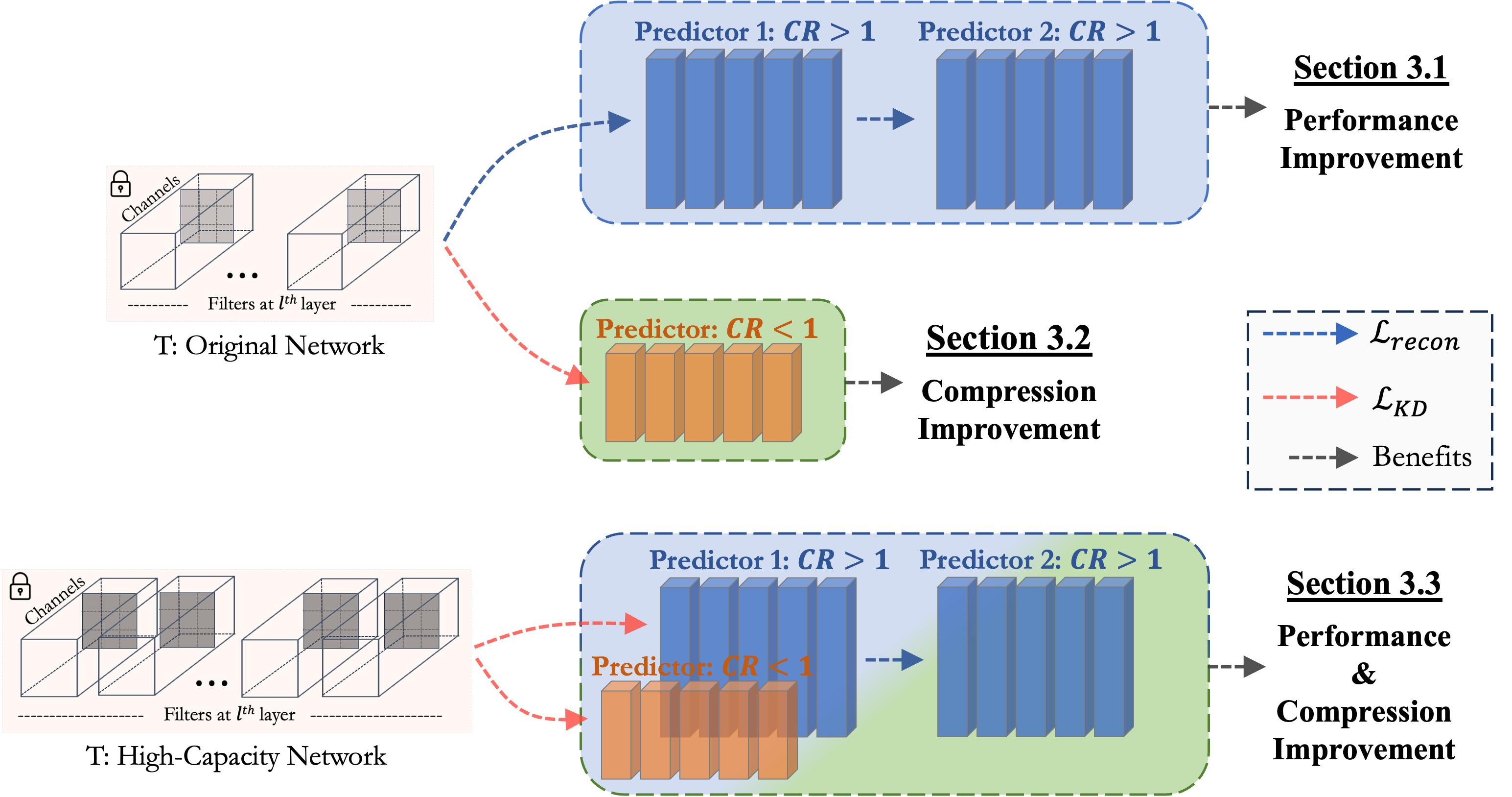
Figure 5: A summary of the explored training schemes and their benefits. We investigate the impact of reconstruction-only setup in Section 3.1, and introduce the decoupled training with separate reconstructed and distillation stages in Section 3.2, which improve storage compression via the more effective predictor networks. Lastly, we demonstrate that a high-capacity teacher can further facilitate both the compression and accuracy goals in Section 3.3.

4 Experiments

In this section, we present experiment results to support the observations made in Section 3 and highlight the practical usage scenarios made possible with our proposed approach. We use benchmark datasets, including CIFAR-10, CIFAR-100 (Krizhevsky et al., 2009), STL-10 (Coates et al., 2011), and ImageNet (Deng et al., 2009). Following a similar setup outlined in (Ashkenazi et al., 2022), we also focus on ResNet architectures (He et al., 2016) as the reconstructed models. Beyond evaluating the in-distribution performance of the reconstructed models, we also assess their robustness using out-of-distribution (OOD) datasets such as CIFAR10-C, CIFAR100-C, and ImageNet-R, and two popular adversarial attacks, FGSM and I-FGSM (Goodfellow et al., 2014). Detailed information about the datasets and training setups is provided in the Appendix D.

4.1 Enhancing Performance Through Progressive Reconstruction - CR$>$1

Firstly, we discovered that the reconstructed model using only the reconstruction loss performs better in testing when weights are predicted by a large predictor ($\textsl{CR}>1$). The reconstruction loss alone enabled the model to improve its performance slightly, with gains ranging from 0.1% to 0.3%. Interestingly, additional rounds of weight prediction further enhanced performance beyond the initial reconstructed model, ultimately achieving gains of up to 0.6%. Table 1 presents the results of the reconstructed models at each round. For example, the first round (Round 1) aims to reconstruct the original network. Then, the second round (Round 2) predicts the weights of the first-round reconstructed model. This process continues progressively through multiple generations until performance improvements plateau. As each round progresses, the predicted weights deviate more from the original solution, as indicated by the increased reconstruction loss. Additionally, the solutions found in each round generally exhibit greater robustness against adversarial attacks than the original network.

Table 1: Evaluation performance of large predictor networks via progressive reconstruction. The reported results are the mean values over three runs.

CIFAR10	Original ResNet20	Hidden 300 (CR$>$1)
		Round 1  Round 2  Round 3  Round 4
Accuracy ($\uparrow$, %)	91.69%	91.79   91.88   91.98   92.00
$\mathcal{L}_{recon}$	-	0.00332  0.00414  0.00500  0.00547
OOD ($\uparrow$, %)	70.49	69.45   69.32   68.82   68.85
FGSM ($\uparrow$, %)	76.41	77.16   77.03   77.08   77.08
I-FGSM ($\uparrow$, %)	75.02	75.56   75.49   75.59   75.69
STL10	Original ResNet56	Hidden 680 (CR$>$1)
		Round 1  Round 2  Round 3  Round 4
Accuracy ($\uparrow$, %)	76.31%	76.40   76.44   76.51   76.54
$\mathcal{L}_{recon}$	-	0.00120  0.00117  0.00125  0.00128
FGSM ($\uparrow$, %	39.28	39.36   39.27   39.30   39.32
I-FGSM ($\uparrow$, %)	36.12	36.13   36.24   36.26   36.17
CIFAR100	Original ResNet56	Hidden 680 (CR$>$1)
		Round 1	Round 2	Round 3	Round 4	Round 5
Accuracy ($\uparrow$, %)	71.37	71.61	71.73	71.85	71.92	71.98
$\mathcal{L}_{recon}$	-	0.00068	0.00082	0.00088	0.00095	0.0010
OOD ($\uparrow$, %)	44.70	44.47	44.75	44.50	44.29	44.47
FGSM ($\uparrow$, %)	44.69	44.83	44.80	45.02	45.23	45.18
I-FGSM ($\uparrow$, %)	39.31	40.91	40.82	41.04	41.21	41.04

4.2 Achieving Greater Compression with Decoupled Training - CR$<$1

Shifting our focus from the previous section, where we used large predictors (CR>1) to improve model performance, we now aim to further compress the predictor size without significantly sacrificing performance. The current training of predictors involves three objectives, as seen in Equation 2, which guide the predictor to effectively mimic the original network. However, in Figure 4(b), we observed that the solution found by Equation 2 was only locally perturbed from the solution in Recon-only model, indicating a restrictive role of the distillation loss. Therefore, we highlight the impact of a simple decoupling of the learning objectives into two phases: a reconstruction phase and a distillation phase, achieving substantial compression gains. To this end, we fine-tune the predictor for a small number of iterations using only $\mathcal{L}_{KD}$, starting from the solution derived by the Recon-only models.

We found that even starting from an inferior point (24.20% from Recon-only on CIFAR-100 in Table 2), performance can be significantly recovered to 69.31% with only $\mathcal{L}_{KD}$ in the second phase, representing a 9% improvement over the Baseline. Furthermore, we achieve a compression ratio of approximately $57\%$ (Hidden $360$) while surpassing the original network’s performance. With these significant improvements compared to the existing baseline, we can achieve better (CIFAR10, CIFAR100) or comparable performance (STL10, ImageNet) with a predictor network smaller than the original network. In the case of ImageNet, we can obtain a $15\%$ compression with only a $3\%$ performance drop compared to the 8% for the baseline.

Table 2: Evaluation performance of small predictor networks via decoupled training. The reported results represent the mean values over three runs except for ImageNet experiments. Recon-only ($\mathcal{L}_{recon}$), Baseline ($\mathcal{L}_{recon}+\mathcal{L}_{KD}+\mathcal{L}_{FMD}$), and Ours ($\mathcal{L}_{KD}$ only in the second phase).

Method	Recon-only / Baseline / Ours
CIFAR10	Original ResNet20	Hidden 120 (CR$\times$100 $\approx$27%)	Hidden 140 (CR$\times$100 $\approx$35%)	Hidden 180 (CR$\times$100 $\approx$53%)
Accuracy ($\uparrow$, %)	91.69	75.75 / 87.99 / 90.75	85.64 / 89.67 / 91.34	90.03 / 91.26 / 91.75
OOD ($\uparrow$, %)	70.49	50.50 / 65.00 / 68.84	60.08 / 67.19 / 69.95	66.34 / 69.75 / 70.48
FGSM ($\uparrow$, %)	76.41	59.76 / 72.73 / 75.38	70.26 / 74.96 / 75.83	74.78 / 76.01 / 76.27
I-FGSM ($\uparrow$, %)	75.02	58.87 / 71.48 / 73.77	69.05 / 73.58 / 74.21	73.39 / 74.44 / 74.83
CIFAR100	Original ResNet56	Hidden 220 (CR$\times$100 $\approx$24%)	Hidden 280 (CR$\times$100 $\approx$36%)	Hidden 360 (CR$\times$100 $\approx$57%)
Accuracy ($\uparrow$, %)	71.37	24.20 / 60.94 / 69.31	49.55 / 66.87 / 70.84	67.48 / 70.39 / 71.46
OOD ($\uparrow$, %)	44.70	13.01 / 38.59 / 43.76	27.08 / 42.00 / 44.61	40.21 / 44.21 / 45.14
FGSM ($\uparrow$, %)	43.69	14.65 / 40.30 / 45.35	30.76 / 43.51 / 44.95	43.28 / 44.82 / 45.01
I-FGSM ($\uparrow$, %)	39.31	14.14 / 38.73 / 42.61	29.38 / 41.41 / 41.95	40.74 / 41.78 / 41.12
STL10	Original ResNet56	Hidden 280 (CR$\times$100 $\approx$36%)	Hidden 320 (CR$\times$100 $\approx$46%)	Hidden 360 (CR$\times$100 $\approx$57%)
Accuracy ($\uparrow$, %)	76.31	69.41 / 74.99 / 76.02	73.36 / 75.64 / 76.25	74.81 / 75.74 / 76.26
FGSM ($\uparrow$, %)	39.28	36.27 / 39.69 / 39.82	38.89 / 39.83 / 39.28	38.53 / 39.77 / 39.21
I-FGSM ($\uparrow$, %)	36.12	33.60 / 36.33 / 36.61	35.44 / 36.27 / 35.96	35.30 / 36.40 / 35.96
ImageNet	Original ResNet18	Hidden 700 (CR$\times$100$\approx$15%)	Hidden 1024 (CR$\times$100$\approx$31%)	Hidden 1372 (CR$\times$100 $\approx$55%)
Accuracy ($\uparrow$, %)	69.76	51.10 / 61.91 / 66.48	65.69 / 67.32 / 68.68	68.81 / 68.87 / 69.32
OOD ($\uparrow$, %)	33.07	19.87 / 25.59 / 30.25	28.36 / 30.90 / 32.17	31.72 / 32.54 / 32.82
FGSM ($\uparrow$, %)	57.83	39.99 / 50.19 / 53.94	53.82 / 55.67 / 56.69	56.96 / 57.14 / 57.40
I-FGSM ($\uparrow$, %)	57.15	38.42 / 49.63 / 53.28	53.23 / 55.06 / 56.09	56.32 / 56.43 / 56.76

4.3 Distillation-Driven Compression and Performance Enhancement - $\textsl{CR}<1$ and $\textsl{CR}>1$

In Sections 4.1 and 4.2, we explored two distinct avenues: improving model performance with large predictors ($\textsl{CR}>1$) and achieving greater compression with small predictors ($\textsl{CR}<1$), respectively. In this section, we seek to simultaneously improve on both of the objectives. Leveraging the flexibility of our decoupled training approach, we can utilize the superior guidance provided by a high-capacity teacher network to enhance parameter efficiency and produce high-fidelity representations. To this end, we employ ResNet50 as a teacher network, which has a size of 90.43MB with $78.48\%$ accuracy on CIFAR100, and the reconstructed network (ResNet56) with a size of 3.25MB. As the teacher network is used only during the training in the second phase, the computational overhead and larger parameter of the teacher do not affect either the predictor network or the reconstructed model.

Firstly, we present the results of a parameter-efficient predictor guided by the teacher network in Table 3. For a fair comparison, the Baseline model is also trained using $\mathcal{L}_{KD}$ under the same teacher’s supervision, as $\mathcal{L}_{FMD}$ is applicable only to architectures that are identical between the student and the teacher. The results in the table support the evidence that a high-performing teacher network can improve the efficiency of the predictor. For instance, in the ‘Hidden 280’ scenario, our method’s performance ‘with guidance’ reveals an accuracy of $72.06\%$. This not only surpasses ‘without guidance’ but also outperforms the original network itself.

Table 3: Evaluation performance of parameter-efficient predictor networks with guidance from a high-performing teacher network (ResNet50). We compare the effect of including the distillation objective to both the baseline ($\mathcal{L}_{recon}+\mathcal{L}_{KD}$), and the proposed approaches ($\mathcal{L}_{KD}$ only in the second phase). In each case, we show the results for without guidance / with guidance.

CIFAR100	Original ResNet56	Hidden 220 (CR$\times$100 $\approx$24%)		Hidden 280 (CR$\times$100 $\approx$36%)		Hidden 360 (CR$\times$100 $\approx$57%)
		Baseline	Ours	Baseline	Ours	Baseline	Ours
Accuracy ($\uparrow$, %)	71.37	60.94 / 58.30	69.31 / 70.25	66.87 / 66.21	70.84 / 72.06	70.39 / 70.94	71.46 / 72.91
OOD ($\uparrow$, %)	44.70	38.59 / 35.45	43.76 / 44.66	42.00 / 41.13	44.61 / 46.20	44.21 / 44.37	45.14 / 47.12
FGSM ($\uparrow$, %)	43.69	40.30 / 37.01	45.35 / 46.69	43.51 / 42.65	44.95 / 47.32	44.82 / 45.53	45.01 / 48.24
I-FGSM ($\uparrow$, %)	39.31	38.73 / 35.68	42.61 / 44.29	41.41 / 40.66	41.95 / 44.29	41.78 / 42.61	41.12 / 44.59

Interestingly, we observe that increasing the predictor size, particularly when parameter efficiency is not a critical factor, can lead to significant performance gains. This is likely due to the ability of a larger predictor to capture higher-fidelity representations of the teacher model. As shown in Table 4, our method achieves superior performance levels the Baseline method cannot reach. Notably, our best-performing model achieves an accuracy of 73.95%, outperforming the conventional KD approach, a student (ResNet56) is trained from scratch using the guidance of ResNet50 teacher network with the $\mathcal{L}_{KD}$ loss, achieving $73.60\%$.

Building on the observation, and aligning with the idea presented in Section 4.1 that additional training complexity can further improve performance, we proceed with one round of progressive reconstruction targeting our best-performing model (73.95%). This resulted in a further improvement to 74.15%.

Table 4: Evaluation performance of large predictor networks with guidance from a high-performing teacher network (ResNet50). We compare the effect of including the distillation objective on both the baseline ($\mathcal{L}_{recon}+\mathcal{L}_{KD}$) and the proposed approaches ($\mathcal{L}_{KD}$ only in the second phase). In each case, we show the results for without guidance / Baseline with guidance / Ours with guidance.

Method	Recon-only / Baseline / Ours
CIFAR100	Original ResNet56	Hidden 510 (CR$>$1)	Hidden 680 (CR$>$1)	Hidden 750 (CR$>$1)
Accuracy ($\uparrow$, %)	71.37	71.45 / 72.02 / 73.41	71.61 / 71.80 / 73.95	71.56 / 71.89 / 73.82
OOD ($\uparrow$, %)	44.70	44.33 / 45.18 / 47.62	44.47 / 45.16 / 47.61	44.93 / 44.66 / 47.74
FGSM ($\uparrow$, %)	43.69	44.32 / 44.02 / 48.75	44.83 / 44.10 / 49.19	44.58 / 44.74 / 49.22
I-FGSM ($\uparrow$, %)	39.31	40.24 / 39.82 / 45.24	40.91 / 39.94 / 45.26	40.35 / 40.55 / 45.53

5 Related Works

Weight generation methods utilizing implicit neural representations (INR) (Ashkenazi et al., 2022), transformer (Knyazev et al., 2023), and diffusion model (Soro et al., 2024) for predicting model weights. NeRN (Ashkenazi et al., 2022) produces an accurate reconstruction of a single network, whereas some other approaches focus on representing the distribution of weights or part of the overall weights.

Weight space manipulation provides a direct way to alter model behavior and comes in a variety of flavors. The recent development of ever larger models (Shoeybi et al., 2019) makes fine-tuning existing models increasingly challenging, as a result, post-training model merging (Matena and Raffel, 2022; Tam et al., 2023; Ilharco et al., 2022) are becoming increasingly popular that combines existing available models for performance enhancement. Besides simply merging the weight, other types of weight manipulation also yield interesting results, e.g., improved model reasoning capability selectively reducing layer rank (Sharma et al., 2023). Apart from manipulating pretrained weights, there are also significant efforts leveraging operation on weight during training, such as stochastic weight averaging (Izmailov et al., 2018; Guo et al., 2023a).

Implicit neural representations or INR (Sitzmann et al., 2020; Tancik et al., 2020) are initially designed for representing low-dimensional data (e.g., 2D or 3D) with complex and potential high-frequency signals. Recently, INR has then been utilized for a variety of domains, e.g., from uncovering correlation in scientific data (Chitturi et al., 2023) to estimating human pose (Yen-Chen et al., 2021). In this work, the predictor network utilizes INR for predicting filter weights for model reconstruction.

Knowledge distillation and pruning has been widely adopted for reducing model size while preserving model performance. Knowledge distillation (Chen et al., 2020; Gou et al., 2021; Chen et al., 2017; Beyer et al., 2022) utilizes a more capable teacher network to transfer prediction behavior to the student network. The pruning techniques (Lee et al., 2019; Liu et al., 2018; Gao et al., 2021; Wang et al., 2021; He and Xiao, 2023) aim to remove non-essential or potentially duplicated functionality in the network and reduce the overall parameter counts.

6 Discussion and Future Work

In this work, we identified effective strategies that significantly improve the accuracy of the reconstructed model and compression ratio for predictor networks through exploring various trade-offs in the parameterization of model weights with neural representation. While effective, one area of the limitations is that the current predictor only works with CNN architectures, restricting its usage. Moreover, despite the flexibility of the proposed protocols that can be combined or re-applied, the necessary additional steps incur more training runs which can lead to a significant increase in computation cost and complexity. However, the increased effort may be worth it to support edge applications where the benefits are multiplied by the number of deployed instances. Still, to help address these challenges, we need methods that can predict weights for diverse architectures and are ideally more efficient when the target model grows in size and complexity. Another interesting direction that is worthy of further investigation is the relationship between the frequency component of the weights and the model’s generalization ability. Could we directly alter the original weights to achieve a similar effect without the need to train a predictor model? Or can we potentially use that insight during training as a regularization that directly improves models’ generalizability?

This work reveals a unique perspective for model improvement and compression through the lens of weight parameterization, which is orthogonal to (i.e., can be arbitrarily combined with) traditional model performance improvement strategies such as stochastic weight averaging or model compression approaches such as distillation and pruning. In this sense, our work is paving the way for interesting and novel combinations of different techniques that are potentially complementary in nature.

7 Acknowledgements

This work was performed under the auspices of the U.S. Department of Energy by Lawrence Livermore National Laboratory under Contract DE-AC52-07NA27344 and was supported by the LLNL-LDRD Program under Project No. 22-SI-020. LLNL-CONF-864812.

Appendix A Code Reproducibility

We plan to release our code upon acceptance of the paper.

Appendix B Decoupled Training with Noise Inputs

In this section, we explore the adaptability of our decoupled training in scenarios where the original task data is unavailable. This investigation aims to address the challenge of operating in a completely data-free environment. We employ uniformly sampled noise as input data, denoted as $X\sim U[-1,1]$. Remarkably, even in the absence of meaningful data, our proposed approach demonstrates significant performance enhancement, with improvements of approximately 2 to 3%.

Table 5: Reconstruction performance of Ours ($\mathcal{L}_{KD}$ only in the second phase) with noise input data

CIFAR10 Method (In-Filter)	Original ResNet20	Hidden 140
		Recon-only	Ours
Size	1.03MB	0.36MB	0.36MB
Acc. ($\uparrow$, %)	91.69%	85.64%$\pm$0.39	87.25%$\pm$0.02
STL10 Method (In-Filter)	Original ResNet56	Hidden 320
		Recon-only	Ours
Size	3.25MB	1.48MB	1.48MB
Acc. ($\uparrow$, %)	76.31%	72.80%$\pm$1.36	74.04%$\pm$0.009
CIFAR100 Method (In-Filter)	Original ResNet56	Hidden 320
		Recon-only	Ours
Size	3.25MB	1.48MB	1.48MB
Acc. ($\uparrow$, %)	71.37%	61.31%$\pm$0.45	64.39%$\pm$0.01

Appendix C Loss Landscape Analysis

Understanding the landscape of the loss function in the weight space provides valuable insights into the optimization process and the behavior of neural networks. Here, we conduct a comprehensive loss landscape analysis to compare the learned weights from each method. As shown in Figure 6, the weights found by our decoupled training lie on the periphery of the most desirable solutions. This suggests that decoupled training enables the predictor to explore better optima by exclusively learning from the predictive knowledge of the original network. Additionally, when examining the gap between train loss and test loss, our method exhibits a smaller gap, aligning with the findings in [Keskar et al., 2017]. This indicates that our approach not only finds better optima but also generalizes well to unseen data.

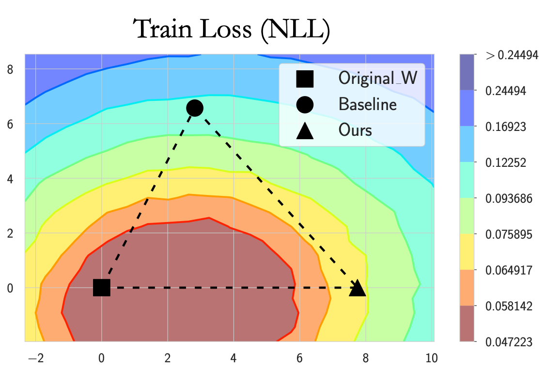
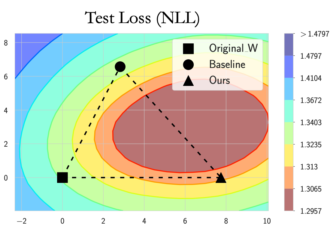
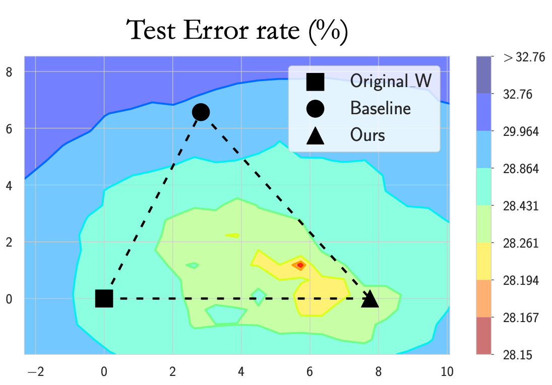
Figure 6: Loss landscape analysis with comparisons among weights from the original networks, Baseline ($\mathcal{L}_{recon}+\mathcal{L}_{KD}+\mathcal{L}_{FMD}$), and Ours ($\mathcal{L}_{KD}$ only in the second phase)

We also conduct the same analysis for Section 3.1. Here, we visualize the loss landscape by interpolating the weights among the original network, and the first and last rounds of the reconstructed model. As shown in Figure 7, all three weights belong to the same local extrema in the loss landscape. This observation is expected since the reconstruction loss constrains all weights to be close to the original model. For the testing loss/error, the reconstruction process appears to enhance the generalization performance.

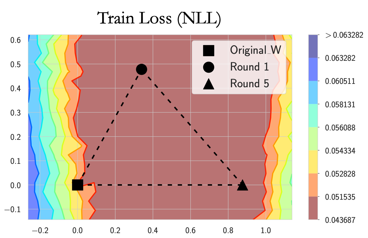
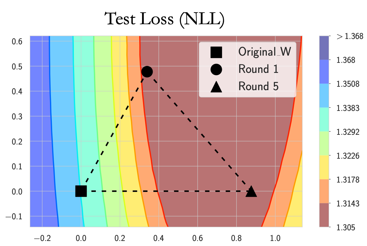
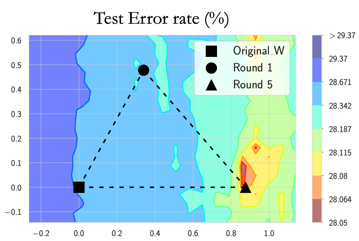
Figure 7: Loss landscape analysis comparing weights from the original network with those from the reconstructed models in the first and last rounds.

Appendix D Datasets and Training Details

D.1 Dataset Description

• CIFAR-10 [Krizhevsky et al., 2009]: The CIFAR-10 dataset consists of 60,000 32x32 color images in 10 classes, with 6,000 images per class. The dataset is divided into 50,000 training images and 10,000 testing images. Each image is labeled with one of the following classes: airplane, automobile, bird, cat, deer, dog, frog, horse, ship, or truck.

• CIFAR-100 [Krizhevsky et al., 2009]: Similar to CIFAR-10, the CIFAR-100 dataset contains 60,000 32x32 color images, but organized into 100 classes, with 600 images per class. The dataset is divided into 50,000 training images and 10,000 testing images. Each image is labeled with one of the 100 fine-grained classes, which are grouped into 20 coarse-grained superclasses.

• STL-10 [Coates et al., 2011]: The STL-10 dataset comprises 10,000 labeled 96x96 color images, with 5,000 images for training and 5,000 for testing. The dataset contains images from 10 different classes: airplane, bird, car, cat, deer, dog, horse, monkey, ship, and truck. Unlike CIFAR, STL-10 also includes a pre-defined unlabeled dataset for unsupervised learning tasks.

• ImageNet-1K [Deng et al., 2009]: ImageNet-1K is a large-scale dataset consisting of over 1.2 million high-resolution images across 1,000 different classes. It is widely used for image classification, object detection, and other computer vision tasks. The dataset is divided into training (1.28 million images), validation (50,000 images), and test sets (100,000 images). Each image is labeled with one of the 1,000 object categories.

D.2 Training Details

Training of Baseline: In baseline training, we follow the same settings outlined in [Ashkenazi et al., 2022]. The Baseline method employs a Multi-layer Perceptron (MLP) with $5$ layers as a predictor, with varying hidden sizes. Training is conducted using the ranger optimizer [Wright, 2019] with a learning rate of $5e-3$. The number of epochs for training is $350$ for CIFAR-10 and STL-10, $450$ for CIFAR-100, and $16\times 10^{4}$ iterations for ImageNet experiments. Similar to minibatch sampling in standard stochastic optimization, during each training step of Baseline, it predicts all reconstructed weights but optimizes only on a mini-batch of them. The weights batch method employed is a random weighted batch, using weighted sampling with a probability of $1-p_{uni}$, where $p_{uni}=0.8$, and a batch size of $4096$ for CIFAR-10, CIFAR-100, and STL-10 datasets. For ImageNet, the experiment was conducted with a minibatch size of $2^{16}$. Hyperparameters $\alpha$ and $\beta$ in learning objectives are set to $1e-5$ for CIFAR-100 and STL-10 datasets, and to $1e-4$ to CIFAR-10, and $1e-6$ for ImageNet. Based on empirical observations, increasing the hyperparameter values during training to emphasize the distillation process causes the Baseline method to experience highly unstable training, often resulting in convergence failure. Therefore, we opted to use the same values as suggested by the authors.

When training predictors, there are two types of permutation-based smoothness: In-Filter and Cross-Filter. Both approaches do not show significant difference in terms of accuracy. The order of weights in the original network remains unchanged; this smoothness only affects the order in which the predictor processes the kernels. In all experiments, In-Filter smoothness was used for CIFAR-10, CIFAR-100, and STL-10 datasets, while Cross-Filter smoothness was employed for the ImageNet dataset.

Training of Progressive-Reconstruction Training: We adhere to the same settings as full training in the Baseline method, including the number of epochs, batch size, learning rate, and other parameters. To isolate and illustrate the reconstruction’s pure effect, the predictor is trained only with the reconstruction loss, $\mathcal{L}_{recon}$. For the next round of progressive-reconstruction training, we select the best-performing models from the previously reconstructed network, determined across three trials with different random seeds, as the target network. If the performance does not surpass that of the target network, we conclude the round. To elucidate the training protocols, we present the results of all three trials conducted on the CIFAR-100 dataset. As observed in the trend of improvement, the gap in enhancement diminishes as the rounds progress.

Table 6: Evaluation performance of large predictor networks via progressive reconstruction. We report all results in three trials. The colored box represents the target performance for the next round.

CIFAR100 Method	# Trial	Original ResNet56	Hidden 680 (CR$>$1)
			Round 1	Round 2	Round 3	Round 4	Round 5
Accuracy ($\uparrow$, %)	1	71.37	71.62	71.73	71.80	71.91	71.92
Accuracy ($\uparrow$, %)	2	-	71.59	71.69	71.89	71.96	72.05
Accuracy ($\uparrow$, %)	3	-	71.63	71.79	71.86	71.91	71.99
mean$\pm$std			71.61%$\pm$0.01	71.73%$\pm$0.04	71.85%$\pm$0.03	71.92%$\pm$0.02	71.98%$\pm$0.05

Training of Decoupled Training: For our proposed decoupled training, we initiate training from the solution obtained by the best-performing model in Recon-only models, as described in Section D.2. As discussed in Section 3.2, fully separating the two phases provides the advantage of enabling more flexible learning during the fine-tuning stage of the second phase. This flexibility allows for the exploration of different optimizers compared to those used in the first phase. Moreover, to maximize the performance of the predictor network, it enables the application of various advanced distillation methods that have been previously explored.

In this experiment, we fine-tune predictors in the second phase for 100 epochs for CIFAR-10, CIFAR-100, and STL-10, and $10^{5}$ iterations for ImageNet, but even with a much smaller number of epochs/iterations, we observe comparable performance. We employ either Adam [Kingma and Ba, 2014] or Ranger [Wright, 2019] optimizers, and in most cases, both yield similar performance. Additionally, in the second phase with $\mathcal{L}_{KD}$, we empirically observed that adding weights to the $\mathcal{L}_{KD}$ with $\alpha<1$ sometimes helps improve convergence, resulting in better performance. Therefore, in most experiments, we set $\alpha$ to $0.01$.

Appendix E Weight Frequency Component Comparison

As observed in the low-frequency analysis, we extend our investigation to the solution obtained in the final round of progressive-reconstruction. The ratio (on the $y$-axis) in this analysis measures the proportion of the total variance (energy) of the matrix $\mathbf{M}$ captured by the first half of the singular values. A higher ratio signifies that the lower frequency components are more dominant. In Figure 8, we present a per-layer comparison of this ratio between the reconstructed and original weights. Despite the presence of noise in the pattern, a clear trend emerges: the reconstructed weights generally exhibit more dominant lower frequency components compared to the original weights, with more pronounced changes occurring in the later layers. Intriguingly, this unexpected finding aligns with observations on rank reduction to enhance the reasoning capabilities of large language models [Sharma et al., 2023], suggesting a broader implication regarding the relationship between the frequency components of weights and model generalizability.

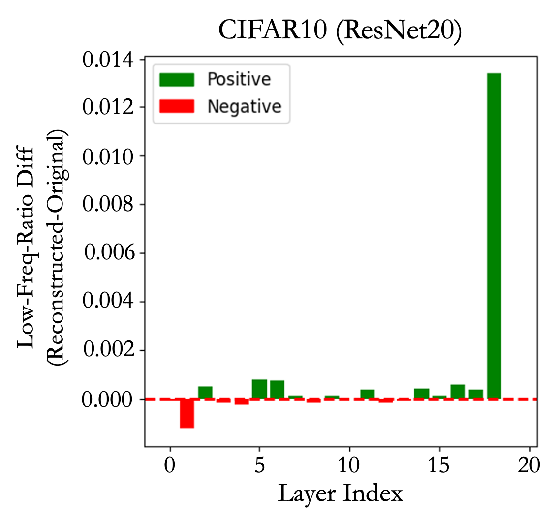
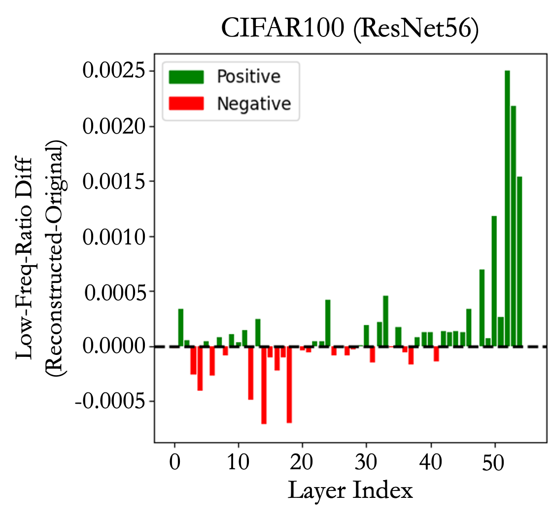
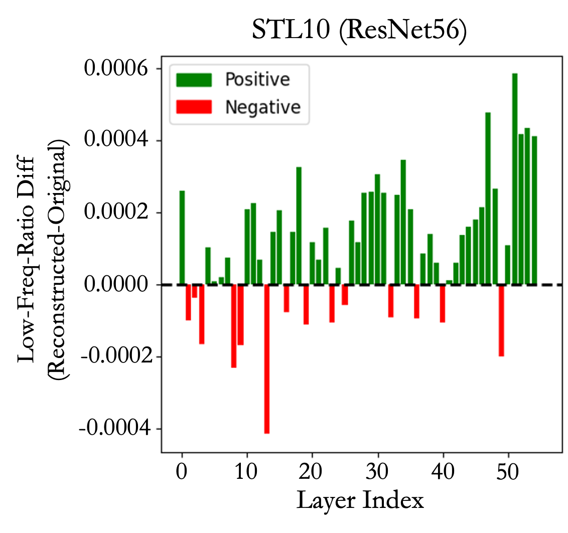
Figure 8: The per-layer of lower frequency component comparison between the original network weight and the reconstructed weight found in the last round of progressive-reconstruction.

Appendix F Interpolation Between Two Extremes

In addition to investigating frequency analysis, we further examine individual pairs of weights by directly interpolating between the original weight $w_{o}$ and each round’s solution from the progressive-reconstruction $\bar{w}$ to gain insight into the relationship between reconstruction error and model accuracy.

Let $w_{o}$ and $\bar{w}_{i}$ represent the original weights and the learned weights at the $i$-th round, respectively. For each value of $\alpha$ in the range $[0,1.0]$, we generate plots showing the test accuracy (on the right $y$-axis) and the corresponding reconstruction error (on the left $y$-axis) for the interpolated weights $f((1-\alpha)w_{o}+\alpha\bar{w}_{i})$. These plots illustrate the performance at intermediate points across different values of $\alpha$, as depicted in Figure 9. The plots reveal a gradual increase in both distance and accuracy as the rounds progress.

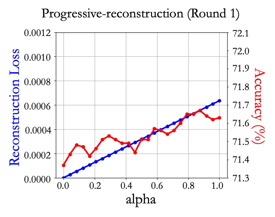
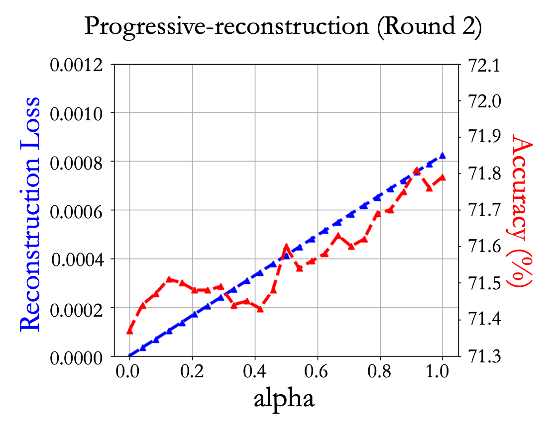
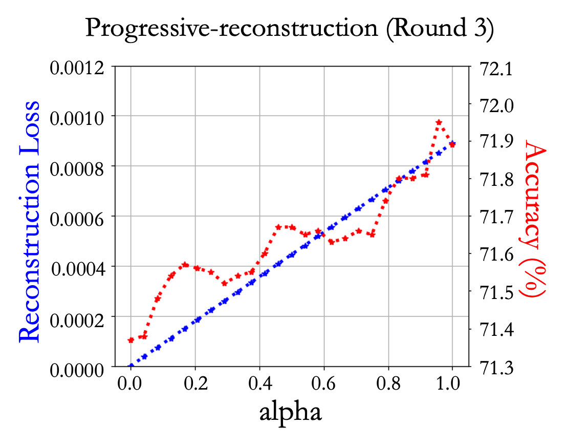
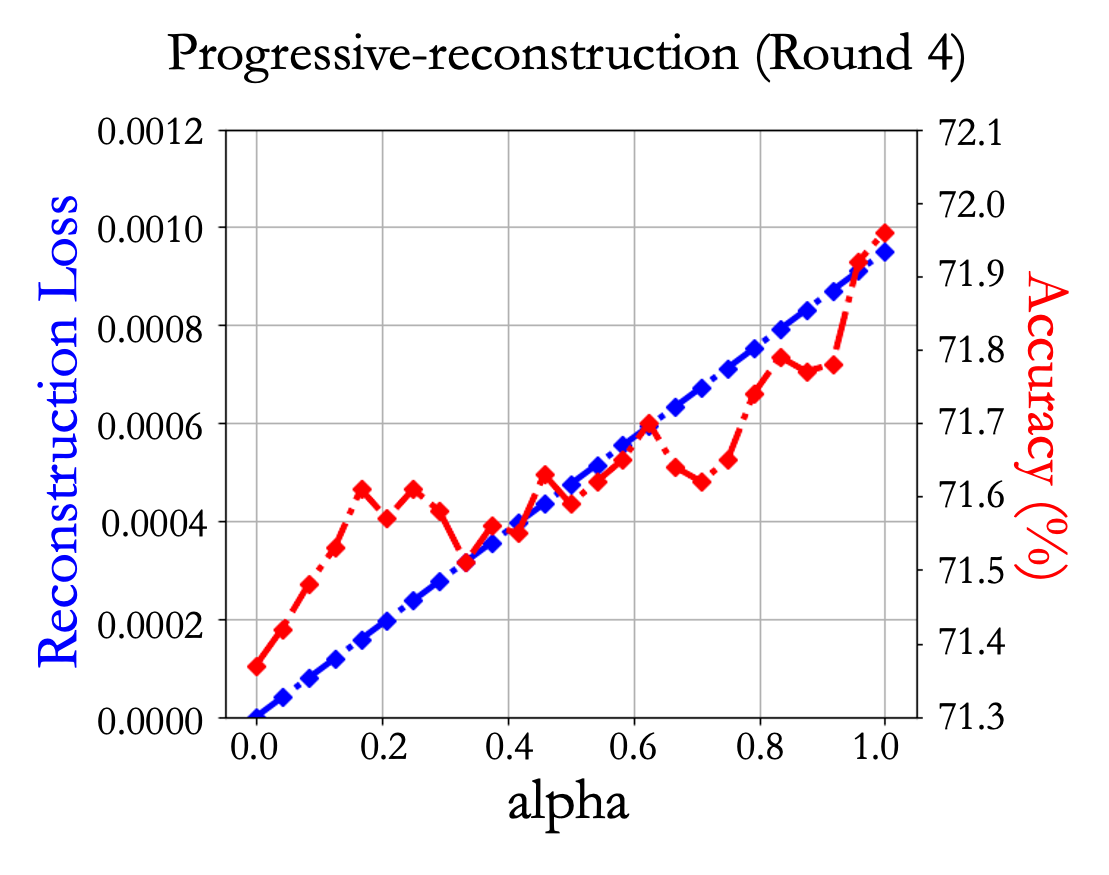
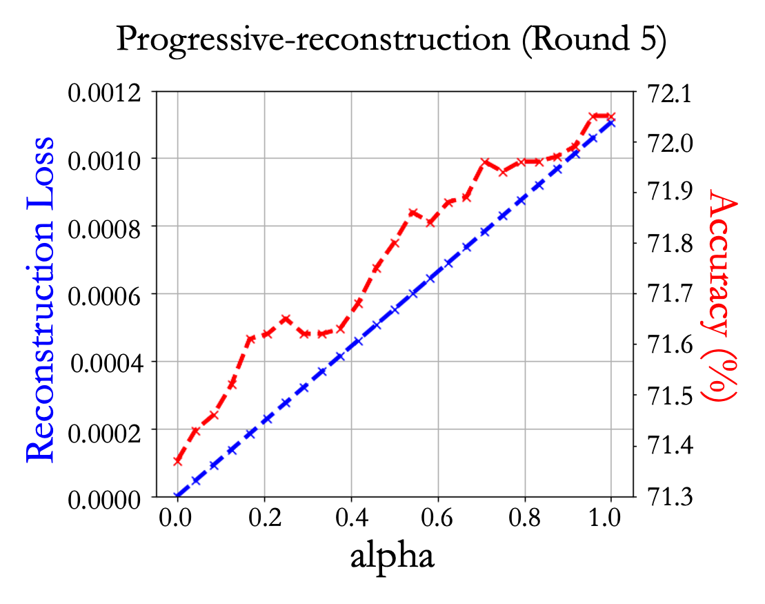
Figure 9: Analysis of interpolation in a 1-D parameter space between the original weight and the solution in each round of progressive-reconstruction.

References

- Ashkenazi et al. [2022] Maor Ashkenazi, Zohar Rimon, Ron Vainshtein, Shir Levi, Elad Richardson, Pinchas Mintz, and Eran Treister. Nern: Learning neural representations for neural networks. In The Eleventh International Conference on Learning Representations, 2022.
- Beyer et al. [2022] Lucas Beyer, Xiaohua Zhai, Amélie Royer, Larisa Markeeva, Rohan Anil, and Alexander Kolesnikov. Knowledge distillation: A good teacher is patient and consistent. In Proceedings of the IEEE/CVF conference on computer vision and pattern recognition, pages 10925–10934, 2022.
- Chen et al. [2020] Defang Chen, Jian-Ping Mei, Can Wang, Yan Feng, and Chun Chen. Online knowledge distillation with diverse peers. In Proceedings of the AAAI conference on artificial intelligence, volume 34, pages 3430–3437, 2020.
- Chen et al. [2017] Guobin Chen, Wongun Choi, Xiang Yu, Tony Han, and Manmohan Chandraker. Learning efficient object detection models with knowledge distillation. Advances in neural information processing systems, 30, 2017.
- Chitturi et al. [2023] Sathya R Chitturi, Zhurun Ji, Alexander N Petsch, Cheng Peng, Zhantao Chen, Rajan Plumley, Mike Dunne, Sougata Mardanya, Sugata Chowdhury, Hongwei Chen, et al. Capturing dynamical correlations using implicit neural representations. Nature Communications, 14(1):5852, 2023.
- Coates et al. [2011] Adam Coates, Andrew Ng, and Honglak Lee. An analysis of single-layer networks in unsupervised feature learning. In Proceedings of the fourteenth international conference on artificial intelligence and statistics, pages 215–223. JMLR Workshop and Conference Proceedings, 2011.
- Deng et al. [2009] Jia Deng, Wei Dong, Richard Socher, Li-Jia Li, Kai Li, and Li Fei-Fei. Imagenet: A large-scale hierarchical image database. In 2009 IEEE conference on computer vision and pattern recognition, pages 248–255. Ieee, 2009.
- Domingos [2012] Pedro Domingos. A few useful things to know about machine learning. Communications of the ACM, 55(10):78–87, 2012.
- Gao et al. [2021] Shangqian Gao, Feihu Huang, Weidong Cai, and Heng Huang. Network pruning via performance maximization. In Proceedings of the IEEE/CVF Conference on Computer Vision and Pattern Recognition, pages 9270–9280, 2021.
- Goodfellow et al. [2014] Ian J Goodfellow, Jonathon Shlens, and Christian Szegedy. Explaining and harnessing adversarial examples. arXiv preprint arXiv:1412.6572, 2014.
- Gou et al. [2021] Jianping Gou, Baosheng Yu, Stephen J Maybank, and Dacheng Tao. Knowledge distillation: A survey. International Journal of Computer Vision, 129(6):1789–1819, 2021.
- Guo et al. [2023a] Hao Guo, Jiyong Jin, and Bin Liu. Stochastic weight averaging revisited. Applied Sciences, 13(5):2935, 2023a.
- Guo et al. [2023b] Yangyang Guo, Guangzhi Wang, and Mohan Kankanhalli. Pela: Learning parameter-efficient models with low-rank approximation. arXiv preprint arXiv:2310.10700, 2023b.
- He et al. [2016] Kaiming He, Xiangyu Zhang, Shaoqing Ren, and Jian Sun. Deep residual learning for image recognition. In Proceedings of the IEEE conference on computer vision and pattern recognition, pages 770–778, 2016.
- He and Xiao [2023] Yang He and Lingao Xiao. Structured pruning for deep convolutional neural networks: A survey. IEEE Transactions on Pattern Analysis and Machine Intelligence, 2023.
- Ilharco et al. [2022] Gabriel Ilharco, Marco Tulio Ribeiro, Mitchell Wortsman, Suchin Gururangan, Ludwig Schmidt, Hannaneh Hajishirzi, and Ali Farhadi. Editing models with task arithmetic. arXiv preprint arXiv:2212.04089, 2022.
- Izmailov et al. [2018] Pavel Izmailov, Dmitrii Podoprikhin, Timur Garipov, Dmitry Vetrov, and Andrew Gordon Wilson. Averaging weights leads to wider optima and better generalization. arXiv preprint arXiv:1803.05407, 2018.
- Keskar et al. [2017] Nitish Shirish Keskar, Dheevatsa Mudigere, Jorge Nocedal, Mikhail Smelyanskiy, and Ping Tak Peter Tang. On large-batch training for deep learning: Generalization gap and sharp minima. In Proceedings of the International Conference on Learning Representations, 2017. URL https://openreview.net/forum?id=H1oyRlYgg.
- Kingma and Ba [2014] Diederik P Kingma and Jimmy Ba. Adam: A method for stochastic optimization. arXiv preprint arXiv:1412.6980, 2014.
- Knyazev et al. [2023] Boris Knyazev, Doha Hwang, and Simon Lacoste-Julien. Can we scale transformers to predict parameters of diverse imagenet models? In International Conference on Machine Learning, pages 17243–17259. PMLR, 2023.
- Krizhevsky et al. [2009] Alex Krizhevsky, Geoffrey Hinton, et al. Learning multiple layers of features from tiny images. 2009.
- Lee et al. [2019] N Lee, T Ajanthan, and P Torr. Snip: single-shot network pruning based on connection sensitivity. In International Conference on Learning Representations. Open Review, 2019.
- Liu et al. [2018] Zhuang Liu, Mingjie Sun, Tinghui Zhou, Gao Huang, and Trevor Darrell. Rethinking the value of network pruning. arXiv preprint arXiv:1810.05270, 2018.
- Matena and Raffel [2022] Michael S Matena and Colin A Raffel. Merging models with fisher-weighted averaging. Advances in Neural Information Processing Systems, 35:17703–17716, 2022.
- Sharma et al. [2023] Pratyusha Sharma, Jordan T Ash, and Dipendra Misra. The truth is in there: Improving reasoning in language models with layer-selective rank reduction. arXiv preprint arXiv:2312.13558, 2023.
- Shoeybi et al. [2019] Mohammad Shoeybi, Mostofa Patwary, Raul Puri, Patrick LeGresley, Jared Casper, and Bryan Catanzaro. Megatron-lm: Training multi-billion parameter language models using model parallelism. arXiv preprint arXiv:1909.08053, 2019.
- Sitzmann et al. [2020] Vincent Sitzmann, Julien Martel, Alexander Bergman, David Lindell, and Gordon Wetzstein. Implicit neural representations with periodic activation functions. Advances in neural information processing systems, 33:7462–7473, 2020.
- Soro et al. [2024] Bedionita Soro, Bruno Andreis, Hayeon Lee, Song Chong, Frank Hutter, and Sung Ju Hwang. Diffusion-based neural network weights generation. arXiv preprint arXiv:2402.18153, 2024.
- Tam et al. [2023] Derek Tam, Mohit Bansal, and Colin Raffel. Merging by matching models in task subspaces. arXiv preprint arXiv:2312.04339, 2023.
- Tancik et al. [2020] Matthew Tancik, Pratul Srinivasan, Ben Mildenhall, Sara Fridovich-Keil, Nithin Raghavan, Utkarsh Singhal, Ravi Ramamoorthi, Jonathan Barron, and Ren Ng. Fourier features let networks learn high frequency functions in low dimensional domains. Advances in neural information processing systems, 33:7537–7547, 2020.
- Wang et al. [2021] Zi Wang, Chengcheng Li, and Xiangyang Wang. Convolutional neural network pruning with structural redundancy reduction. In Proceedings of the IEEE/CVF conference on computer vision and pattern recognition, pages 14913–14922, 2021.
- Wright [2019] Less Wright. Ranger-a synergistic optimizer. GitHub Repos. Available online at: https://github. com/lessw2020/Ranger-Deep-Learning-Optimizer, 2019.
- Yen-Chen et al. [2021] Lin Yen-Chen, Pete Florence, Jonathan T Barron, Alberto Rodriguez, Phillip Isola, and Tsung-Yi Lin. inerf: Inverting neural radiance fields for pose estimation. In 2021 IEEE/RSJ International Conference on Intelligent Robots and Systems (IROS), pages 1323–1330. IEEE, 2021.