Global decomposition of networks into multiple cores formed by local hubs

Abstract

Networks are ubiquitous in various fields, representing systems where nodes and their interconnections constitute their intricate structures. We introduce a network decomposition scheme to reveal multiscale core-periphery structures lurking inside, using the concept of locally defined nodal hub centrality and edge-pruning techniques built upon it. We demonstrate that the hub-centrality-based edge pruning reveals a series of breaking points in network decomposition, which effectively separates a network into its backbone and shell structures. Our local-edge decomposition method iteratively identifies and removes locally least important nodes, and uncovers an onion-like hierarchical structure as a result. Compared with the conventional $k$-core decomposition method, our method based on relative information residing in local structures exhibits a clear advantage in terms of discovering locally crucial substructures. Furthermore, we introduce the core-periphery score to properly separate the core and periphery with our decomposition scheme. By extending the method combined with the network community structure, we successfully detect multiple core-periphery structures by decomposition inside each community. Moreover, the application of our decomposition to supernode networks defined from the communities reveals the intricate relation between the two representative mesoscale structures.

I Introduction

Networks have attracted considerable attention across various fields due to their inevitable omnipresence in nature and society [1, 2, 3]. Consisting of nodes for individual objects of our interest and edges connecting them, a network succinctly represents an interacting system, which is a quintessential topic of statistical mechanics [4]. Compared with traditional topics of statistical mechanics, perhaps a notably distinct feature of the recently developed theory of highly heterogeneous or “complex” networks is the existence of a few dominant elements that can govern the entire system. The identification of such important nodes and their disproportionately significant influence have been studied extensively [1, 2, 3, 4]. One noticeable example in terms of both popularity and significance is the number of the nearest neighboring nodes for each node, which is called the degree. It affects a number of key aspects of networks, e.g., the robustness under failures and attacks [5, 6, 7], the epidemic spreading [8], critical phenomena [9], the controllability [10], etc.

Roughly, there are two streaks of research for identifying important nodes with large degrees within a network: one focuses on individual nodes, e.g., by detecting the ones with large degrees or many connections to the rest of the network, usually dubbed as “hubs” [11], and the other identifies a group of important nodes, e.g., by detecting “core” nodes that are well connected to both each other inside and outside the group  [12, 13, 14, 15, 16, 17, 18, 19, 20, 21, 22]. In contrast to the simplest concept of hub nodes by globally counting their neighbors, when it comes to the core node groups, individual nodes’ degree relative to their peers in the group is also crucial. The latter is precisely captured by the measure called “hub centrality” introduced in the series of previous works [23, 7] by some of the authors of this paper, to detect such local hubs in the context of game theory and cascading failure. The hub centrality, defined as the normalized rank of each node within the node group composed of the node itself and its nearest neighbors in terms of degree, successfully identifies locally important nodes. Both global and local hubs play profound roles across various dynamical systems, such as cascading failure [7, 24, 25], disease spreading [12], vaccination [26], and evolutionary game theory [27], according to their unique characteristics.

In this regard, we would like to point out that most of conventional methods to detect core nodes in networks [12, 13, 14, 15, 16, 17, 18, 19, 20, 21, 22] almost exclusively utilizes the concept of global connections in terms of degree, without enough consideration of nodes’ relative position within their neighbor groups. Well-known examples include the decomposition of networks based on degrees, or the k-core decomposition, which iteratively removes nodes with fewer than k connections until only nodes with at least k connections remain [12, 13]. Another related decomposition is the identification of the core-periphery structure [14, 15, 16, 17, 18, 19, 20, 21, 22] by detecting the core nodes with statistically dense connections to the entire network and treating the rest as periphery. For all of these approaches, one simply takes a degree of a node as a face value without consideration of its aforementioned relative position. When there are a variety of local groups in heterogeneous sizes, however, as many real-world networks would actually be so, a particular degree value can make a locally strong hub that governs the entire dynamical property near the hub belonging to a small group, while the same degree value may correspond to a mediocre node belonging to a much larger group. In other words, the mixture of heterogeneous degree distributions [2] and heterogeneous locally dense structures or “communities” [28, 29, 30] requires a meticulous approach to decomposing a network using nodes’ degree as a tool.

By discriminating the differential effects of the global and local hubs or cores, it would be possible to significantly enhance our understanding of both structural and dynamical aspects of networks. In this paper, we introduce the local-edge decomposition, which is based on the product of hub centrality values of the nodes connected by the edge of interest. One particularly promising aspect of this hub-centrality-based edge-pruning process is the presence of a natural breaking point between the zero and nonzero edge-importance values, detected by the giant component size, and we take the series of such breaking or cusp points to build a systematic procedure to decompose a network. It assigns nodes’ hierarchical levels and uncovers the onion structure of networks [31].

Because we use the concept of local hubs, our decomposition scheme takes a unique viewpoint of putting local hubs in the highest hierarchical level, and this perspective will open new possibilities of applications. Among the possibilities, we study and propose the core-periphery structure and the score function to find it, based on the nodes’ local-hub-based hierarchical levels. We finalize the paper by extending our method by both zooming-in and zooming-out—core-periphery structures within communities and coarse-graind supernode networks, which may provide a crucial clue to solve the conundrum of the necessity for “something else” in core-periphery [20] by finding multiple cores composed of local hubs.

II Decomposition of networks

The notion of network decomposition in this study refers to the process of extracting the most essential part of a network by iteratively peeling the relatively less important parts [12, 13]. It allows for the identification and focused study of the most critical parts of the network, such as key infrastructure nodes in a power grid that, if failed, could cause widespread outages [32], or influential individuals in a social network who can significantly impact the spread of information or diseases [33]. This targeted approach facilitates a deeper understanding and more detailed analysis of key components, ultimately leading to improved network performance and resilience. In this section, we provide the result of edge pruning based on different criteria, introduce a local-hub-based strategy as our main scheme, and compare it with the conventional k-core decomposition based on global degree values [12, 13].

II.1 Edge pruning and cusp point

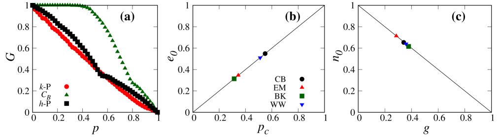
Figure 1: (a) The giant component size $G$ as a function of the fraction $p$ of removed edges. The network is a collaboration network in the field of computational geometry. (b)–(c) The fraction $e_{0}$ of edges with $\mathscr{E}^{h\mbox{-}\mathrm{P}}=0$ and the fraction $n_{0}$ of nodes with $h=0$ as a function of the cusp point $p_{c}$ and the giant component size $g$ with zero hub-centrality nodes removed, respectively. Each point represents the outcome of each individual network listed in Table 1. The solid lines in (b) and (c) represent $e_{0}=p_{c}$ and $n_{0}=1-g$, respectively.

To quantify edges’ importance to set the criterion for decomposition, we try edge betweenness centrality related to the shortest-path-based global transport dynamics [34] and the product of nodes’ importance, which are attached to both ends of the edge. In the latter case, the property of an edge that connects nodes $i$ and $j$ is given by the product of values assigned to each edge as

$$\mathscr{E}_{ij}=\psi_{i}\psi_{j}\,,$$ (1)

where $\psi_{i}$ is a certain property of node $i$. In this paper, we try the degree representing the global connectivity and the hub centrality from the normalized local rank in connectivity [23, 7] proposed by some of the authors of this paper. The hub centrality of a node is the fraction of its neighbors with lower degrees than the node [23, 7]. In other words, we first examine the effects of three types of edge importance for pruning edges for network decomposition: the edge betweenness centrality ($C_{B}$) [1, 2, 3] by directly setting $\mathscr{E}^{C_{B}}_{ij}\equiv C_{B}(i,j)$, the degree product ($k\mbox{-}\mathrm{P}$) by setting $\mathscr{E}^{k\mbox{-}\mathrm{P}}_{ij}=\psi_{i}\psi_{j}$ where $\psi_{i}\equiv k_{i}$ (the degree of node $i$), and hub-centrality product ($h\mbox{-}\mathrm{P}$) by setting $\mathscr{E}^{h\mbox{-}\mathrm{P}}_{ij}=\psi_{i}\psi_{j}$ where $\psi_{i}\equiv h_{i}$ (the hub centrality of node $i$).

In our edge-pruning strategy, we calculate the set of edge importance $\{\mathscr{E}_{ij}\}$ in the original network and use it throughout the process until the end. We do not recalculate the hub centrality and its product during the edge removal process, as it is not our main interest to investigate the modified structure itself ; rather, we would like to extract more central parts in terms of the edge importance in the original structure as we proceed. We implement repeated edge pruning , which removes the least important edges at each time step. We first examine a natural measure to characterize the edge-pruning process, which is the relative giant (i.e., the largest connected) component size $G$ of the remaining structure with respect to the original network size, as a function of the fraction $p$ of removed edges. To focus on the fragmentation caused by the edge-pruning process, for all of our numerical studies, we use the giant component of the original networks (the sizes of which are listed inside the parentheses in Table 1) in the beginning.

Table 1: Information of real-world networks considered in the work: number of nodes ($N$), giant component size ($G$), number of edges ($E$), number of edges of the giant component ($E_{G}$), average degree ($\langle k\rangle$), average degree of the giant component ($\langle k\rangle_{G}$), average local clustering coefficient ($c_{l}$), and assortativity ($r$). When implementing local-edge decomposition, it is conducted within the giant component $G$. The collaboration network is the authors’ collaboration network in the field of computational geometry.

Networks	$N$ ($G$)	$E$ ($E_{G}$)	$\langle k\rangle$ ($\langle k\rangle_{G}$)	$c_{l}$	$r$	Ref.
Collaboration (CB)	$6\,158$ ($3\,621$)	$11\,898$ ($9\,461$)	$3.864$ ($5.225$)	$0.485$	$0.242$	[37]
Email (EM)	$33\,696$ ($33\,696$)	$180\,811$ ($180\,811)$	$10.731$ ($10.731$)	$0.509$	$-0.116$	[38]
Brightkite (BK)	$58\,228$ ($56\,739$)	$214\,078$ ($212\,945$)	$7.353$ ($7.506$)	$0.172$	$0.010$	[39]
Wikipedia word (WW)	$146\,005$ ($145\,145$)	$656\,999$ ($656\,230$)	$8.999$ ($9.042$)	$0.602$	$-0.062$	[40]

A typical example is the case of the collaboration network in the field of computational geometry (CB) [37] (see Table 1 for basic statistics) shown in Fig. 1(a). In the case of $k\mbox{-}\mathrm{P}$, $G$ decreases monotonically. For $C_{B}$, the value of $G$ remains high when $p\lesssim 0.4$, but $G$ decreases rapidly once $p\gtrsim 0.4$. In contrast to previous cases, $h\mbox{-}\mathrm{P}$ shows a cusp point ($p_{c}$), which is the point where the rate of change in $G$ abruptly changes; the slope of $G(p)$ suddenly drops when $p$ crosses the value $p_{c}$. Other networks listed in Table 1 also have the cusp point when the edges are removed by $h\mbox{-}\mathrm{P}$ and show qualitatively similar behavior to Fig. 1(a). This seemingly puzzling behavior is, in fact, simply explained, with the hint from the observation of the fraction $e_{0}$ of edges with exactly null importance, i.e., the edges with $\mathscr{E}^{h\mbox{-}\mathrm{P}}=0$, which are precisely the edges connecting at least one node with the locally smallest degree: $h_{i}=0$ by the product rule. As shown in Fig. 1(b), for all of the four real networks we examine, the $e_{0}$ value coincides with the cusp point $p_{c}$ for each network. This implies that the transition between $p<p_{c}$ and $p>p_{c}$ corresponds to the part where the edges with $\mathscr{E}^{h\mbox{-}\mathrm{P}}=0$ are removed (by our edge-pruning rule, they must be removed first) versus the part where the rest of the edges with $\mathscr{E}^{h\mbox{-}\mathrm{P}}>0$ are removed.

Moreover, for any node $i$ with $h_{i}=0$, by definition, all of its neighboring nodes should have larger degrees than $k_{i}$, so $\mathscr{E}^{h\mbox{-}\mathrm{P}}_{ij}=0$ for any node $j$ connected to $i$. As a result, all of the edges connected to $i$ will be removed during the $p<p_{c}$ pruning process. Conversely, as already stated, each of the edge-removal processes for $p<p_{c}$ involves such a node with $h_{i}=0$. Therefore, the edge-pruning process for $p<p_{c}$ exactly corresponds to the process of pinpointing the nodes with $h_{i}=0$ and removing all of their edges. This surgical removal effectively isolates those locally least important nodes and leaves the rest of the network as a new giant component precisely at $p=p_{c}$. In principle, it is possible for a node with nonzero hub centrality to be isolated as a result of the removal of all of its neighbors with $h=0$ even for $p<p_{c}$ . However, one can check that the relation $g=1-n_{0}$ holds (under the assumption of the absence of such cases; in general, $g<1-n_{0}$ caused by the possibility of the aforementioned “casualty” node with $h>0$) for our empirical networks, where $n_{0}$ is the fraction of the nodes with $h_{i}=0$ and $g\equiv G(p=p_{c})$ is the fraction of the giant component remaining at $p=p_{c}$, from Fig. 1(c). In other words, the separation of zero-hub-centrality nodes does not cause the noticeable separation of other nodes with nonzero hub centrality from the giant component up to $p=p_{c}$, and most nodes with $h>0$ belong to the new giant component at $p=p_{c}$.

From these observations, we deduce that a network composed of a single giant component harbors a one-step deeper-level giant component formed by positive hub-centrality nodes inside and zero hub-centrality nodes (along with a negligible fraction of positive hub-centrality nodes) attached to it outside. In terms of transport property, if we choose two different zero hub-centrality nodes, as each of them is likely to have a neighbor with $h>0$, there is usually at least a path only through nonzero hub-centrality nodes, which is reminiscent of the backup-pathway-based notion of core-periphery [42, 43] and highlights the role of the giant component at $p=p_{c}$ as a structural and dynamical backbone. On that threshold, the network is divided into a backbone composed of nodes with $h>0$ and a shell mostly composed of nodes with $h=0$.

II.2 Local-edge decomposition and node hierarchy

Figure 2: (a)–(c) The giant component size $G$ as a function of the fraction $p$ of removed edges based on the hub-centrality product ($h\mbox{-}\mathrm{P}$). (a) The original collaboration network used in Fig. 1. (b) The backbone of the original network. (c) The backbone of the original network’s backbone. (d) The fraction $n_{0}$ of zero hub-centrality nodes as a function of the relative fraction $g$ of the giant component size with zero hub-centrality nodes removed in decomposed networks. The solid line represents $n_{0}=1-g$, which implies the set of zero hub-centrality nodes $\approx$ the shell at each decomposition level.

The clear-cut separation between the backbone and the shell described in Sec. II.1 provides us a nice natural cutoff to examine the locally important component. Then, why do we just stop there? We can use the process repeatedly, by applying the same procedure to the backbone as a new network for decomposition, and so on. For the backbone [the giant component at the cusp point $p_{c}^{(1)}$ in Fig. 2(a)], we recalculate the hub-centrality values for each node and implement the same edge-pruning process by the $h\mbox{-}\mathrm{P}$ rule. Figure 2(b) shows the results of such second-level edge-pruning, and we can observe a cusp point again, as in the original network Fig. 2(a). Not surprisingly, it occurs as a number of nodes with $h>0$ in the original network have now become nodes with $h=0$ in the first-level backbone. Accordingly, the first-level backbone is once again separated into the second-level backbone and shell. In the second-level backbone, which is the giant component at $p=p_{c}^{(2)}$ of Fig. 2(b), we recalculate hub centrality and implement the edge-pruning process again. As expected, it shows a cusp point at $p=p_{c}^{(3)}$ (the third level) as shown in Fig. 2(c).

We can continue this backbone-extraction process by removing the edges with $\mathscr{E}^{h\mbox{-}\mathrm{P}}=0$ at each level until all of the nodes are isolated. We refer to this process as the local-edge decomposition (LED). For the readers, we provide the following step-by-step guide for numerical simulation:

1. Initial Calculation: Calculate the hub centrality of each node in the network (level $l=0$).

2. Edge Pruning: For each level $l$, identify and remove all of the edges where the product of hub centrality values is zero, i.e., $\mathscr{E}^{h\mbox{-}\mathrm{P}}=0$. When there is no edge with $\mathscr{E}^{h\mbox{-}\mathrm{P}}=0$ remaining, the fraction $p$ of removed edges is equal to $p_{c}$ at level $l$ and the remaining giant component becomes the new network at level $(l+1)$.

3. Recalculation: At the beginning of each new level $(l+1)$, recalculate the hub centrality for the new network at level $(l+1)$.

4. Iteration: Repeat the edge-pruning and recalculation process described in 2 and 3 above by increasing level $l$.

5. Termination: Continue this iterative process until no more edges can be removed (i.e., all nodes are isolated).

To verify our earlier argument $n_{0}\approx 1-g$ (for $p<p_{c}$, the edges are eliminated if and only if $\mathscr{E}^{h\mbox{-}\mathrm{P}}=0$) at each level, we show all of the $(n_{0},g)$ pairs calculated at each level on top of the line $n_{0}\approx 1-g$, and one can observe the excellent agreement. The other networks listed in Table 1 also show qualitatively similar results to Fig. 2. The final level is composed of nodes with the same degree and the edges with $\mathscr{E}^{h\mbox{-}\mathrm{P}}=0$ (no node’s degree can be smaller than any other nodes’ degree), so the whole process is naturally terminated by the elimination of the entire edges altogether along with all of the nodes; generally, it forms a clique in real-world networks according to our observation. Therefore, we conclude that a network can be decomposed as an onion-like structure [31], wherein we extract the core of the onion by removing locally least important nodes iteratively through LED.

As an illustration of this iterative LED, we show a simple example in Fig. 3, where different colors (and edge thickness) represent the decomposition level. The green nodes have zero hub centrality and are connected to the green edges with $\mathscr{E}^{h\mbox{-}\mathrm{P}}=0$, and they are decomposed first. At the decomposed network, which is composed of blue and red nodes, we recalculate hub centrality and remove the blue edges with $\mathscr{E}^{h\mbox{-}\mathrm{P}}=0$. As a result, the blue nodes are decomposed, and only the red nodes that form a $4$-clique with the red edges remain, which will eventually be removed at the next level. In other words, the green, blue, and red nodes are hierarchically organized to constitute levels $0$, $1$, and $2$, respectively.

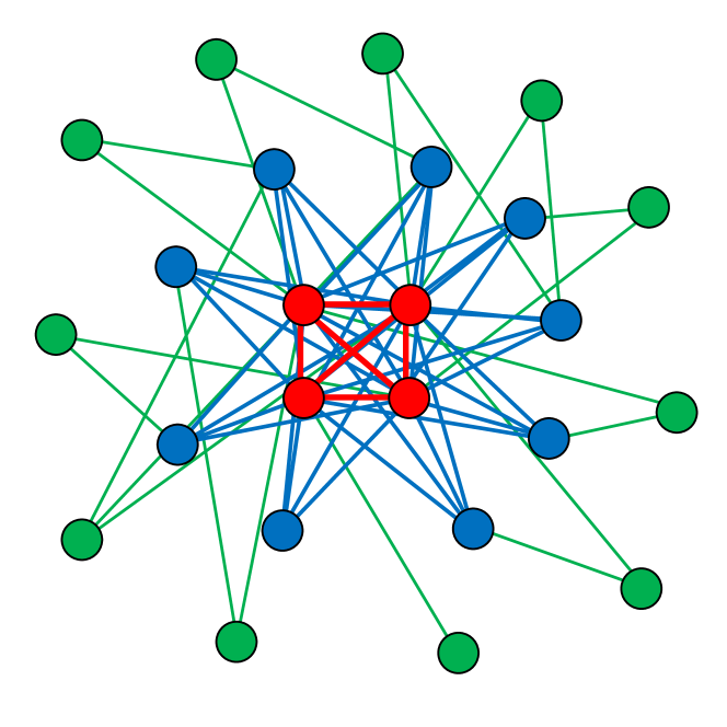
Figure 3: An example network to illustrate the LED decomposition. The nodes filled with the same color belong to the same hierarchical level. The green, blue, and red nodes belong to the lowest, intermediate, and highest levels, respectively. The color and thickness of the edges indicate the decomposition levels as well.

II.3 Comparison with the k-core decomposition

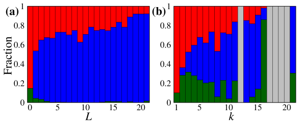
Figure 4: The fraction of the level (or “shell” in the kCD) relationship between nodes and their neighbors. The colors red, blue, and green indicate that nodes at a given level have neighbors with higher, lower, or the same level, respectively. The regions filled with gray represent the absence of nodes in the corresponding levels. The panel (a) is for the LED, and the panel (b) is for the kCD.

Our decomposition scheme will obviously remind anyone familiar with network science of the celebrated k-core decomposition (kCD) [44, 12, 13]. The kCD is one of the early established methods to extract the most central part of a network, by iteratively removing the smaller-degree nodes. Starting from $k=1$, it peels out nodes with the minimum degree until no node has a degree smaller or equal to $k$ at each stage (the removed nodes for a given value of $k$ are called the $k$-shell, analogous to the “level” in our LED) , and continues this process by increasing $k$ until all of the nodes are removed; in this way, nodes are hierarchically decomposed as in our LED, with a similar final stage composed of a clique to ours.

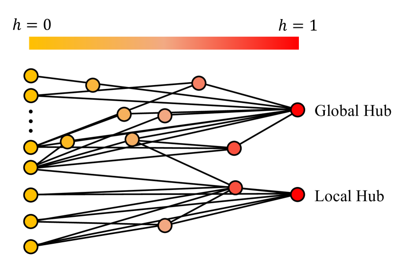
Figure 5: A schematic illustration of examples of global and local hubs, whose horizontal location is aligned with their hub-centrality values represented with the horizontal color bar with gradation.

Despite the similarity, however, the crucial difference between the kCD and our LED comes from the fact that the kCD is based on degree (global information), and our LED is based on hub centrality (local information). One way to see the difference is to observe the inter-level connections. Figure 4 shows how nodes included in a given level are connected to other-level nodes for the CB network. In the case of LED, as shown in Fig. 4(a), the overall tendency indicates that higher-level nodes are connected to lower-level nodes naturally, but the connections between the same-level nodes are quite rare except for a few lowest levels. This happens because the same-level connections correspond to the edges connecting the two distinct zero hub-centrality nodes in a given level, which is only possible when the two nodes have exactly the same degree and both of them should have the lowest degree among their neighbors. In other words, the LED is a systematic way to find the edges essentially separating different hierarchical levels of network organization. For kCD, in contrast, there are a substantial number of connections between the same-level nodes as shown in Fig. 4(b), because the nodes in the $k$-shell would just mean a similar edge density in the area regardless of the local degree gradient with respect to the neighbors.

An illustrative way to see the stark difference between the LED and the kCD is presented in Fig. 5. In the LED, the highest-level nodes are local hubs with $h\approx 1$ regardless of their degree values themselves, so the decomposition process gradually prunes edges simultaneously in substructures (e.g., communities) with various different scales. This property will play a crucial role in dealing with multiple core-periphery structures later. In contrast, if the kCD were used, the local hub would be removed much earlier than the global hub, so observing the local organizational structure with different scales would be much harder. In addition, because the LED uses the local relative information, the nodes in a network are naturally composed of consecutive nonempty levels as shown in Fig. 4(a). In contrast, for the kCD using the absolute degree values, it is possible for a certain $k$-shell to be empty as shown in the gray parts in Fig. 4(b). As a result, for most cases, we obtain a more gradual decomposition of a network for the LED, compared with the kCD. This is another advantage of using the LED, which provides more granular information about network organization.

III Core-Periphery Structure of networks

The core-periphery structure (CP) [14, 15, 16, 17, 18] is another fundamental mesoscale structure of networks regarding the gradually sparser or denser parts in a network; it implies that a network consists of a dense “core” and sparse “periphery.” Most early-day studies on the CP assume the existence of a single core and the periphery surrounding it understandably because it is simplest. However, recent studies started to acknowledge that for networks to have a nontrivial CP other than the one that can easily be separated by the degree values, it is essential to have a complicated CP composed of multiple cores (and not surprisingly, most real networks are “complex” enough to do so) [19, 20, 21, 22]. Considering the ubiquitous existence of community structures [28, 29, 30], it is also reasonable to assume the presence of multiple cores. Our LED scheme is able to detect such structures, as we will present from now on.

III.1 Core-periphery structure and score

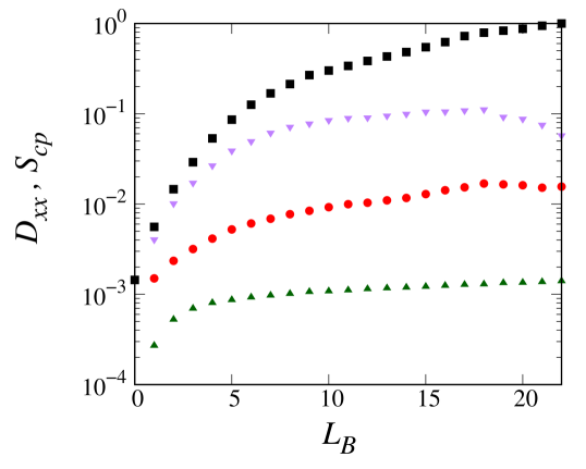
Figure 6: The connection densities of core-core, core-periphery, and periphery-periphery, along with the core-periphery score, as a function of the boundary level $L_{B}$. The black (square), red (circle), and green (triangle) points represent the connection densities of core-core, core-periphery, and periphery-periphery, respectively. The purple (inverse triangle) points indicate the core-periphery score. At $L_{B}=0$, the connection densities for core-periphery and periphery-periphery, as well as the core-periphery score, are zero. The core-periphery score reaches its maximum at $L_{B}=18$.

First, in order to demonstrate that our LED identifies the single CP, we observe the connection density of core-core ($D_{cc}=2M_{cc}/[N_{c}(N_{c}-1)]$), core-periphery ($D_{cp}=M_{cp}/(N_{c}N_{p})$), and periphery-periphery ($D_{pp}=2M_{pp}/[N_{p}(N_{p}-1)]$) edges, where $N_{c}$, $N_{p}$, $M_{cc}$, $M_{cp}$, and $M_{pp}$ correspond to the number of core nodes, that of periphery nodes, that of edges connecting core nodes, that of edges connecting core and periphery nodes, and that of edges connecting periphery nodes, respectively. The conventional notion of CP suggests the inequality [14, 15, 16, 17, 18]

$$D_{cc}>D_{cp}>D_{pp}\,.$$ (2)

We implement the LED in a network, classify nodes according to the hierarchical level $L$ as in Sec. II.2, and treat higher-level nodes as the core part. The key question is then to set the boundary between the core and the periphery, i.e., to propose a threshold value $L_{B}$, where the nodes in the levels $L\geq L_{B}$ and those in the levels $L<L_{B}$ are categorized as the core and periphery parts, respectively. According to Fig. 6 for the CB network, for any value of $L_{B}$, the CP condition in Eq. (2) is satisfied. As demonstrated in Sec. II.2, the nodes with the lowest relative degree in local neighbors are the first to be decomposed from the giant component, leading to higher connection densities among higher-level nodes compared with lower-level nodes.

To decide the most appropriate value of $L_{B}$ to accurately distinguish the CP, we introduce a core-periphery score $S_{cp}$ based on the following two conditions that we consider as the most ideal CP.

1. The core nodes are fully connected to each other.

2. All of the periphery nodes are connected to core nodes, and no edges between periphery nodes exist.

Basically, it represents an adjacency matrix with the perfect shape. The condition $1$ is quantified with $D_{cc}$, and the condition $2$ is measured by $M_{cp}/N_{p}$. The quantity $M_{cp}$, the number of edges connecting the core and periphery nodes, is also the number of periphery nodes connected to core nodes for a simple network, so the ratio $M_{cp}/N_{p}$ represents the fraction of periphery nodes that are connected to the core nodes. In other words, the extent to which the core and periphery nodes satisfy the above two conditions is determined by $D_{cc}$ and $M_{cp}/N_{p}$, respectively. To quantitatively assess the core-periphery structure using these criteria, we define the core-periphery score as,

$$S_{cp}\equiv D_{cc}\frac{M_{cp}}{N_{p}}-D\,\mathrm{min}\{1,DN_{c}\}\,,$$ (3)

where $D=2(M_{cc}+M_{cp}+M_{pp})/[(N_{c}+N_{p})(N_{c}+N_{p}-1)]$ is the density of the entire network. This represents the difference between the actual similarity and the expected similarity by chance as the null-model case, concerning the ideal CP. The core-periphery score is maximized when both conditions are satisfied, thus it helps to identify the most optimal boundary level $L_{B}^{*}$ for distinguishing between the core and periphery of a network. As the boundary level $L_{B}$ increases from $1$ to $18$ ($S_{cp}$ for $L_{B}=0$ is undefined), the distinction between core and periphery nodes becomes clearer, causing the core-periphery score to gradually increase. At $L_{B}^{*}=18$, the core-periphery score reaches its maximum value, and this means that nodes belonging to $L\geq L_{B}^{*}=18$ form the core, while the remaining nodes form the periphery in this network. However, when $L_{B}$ exceeds $L_{B}^{*}=18$, $M_{cp}$ decreases and the core-periphery score starts to decrease.

Despite the existence of optimal boundary $L_{B}^{*}=\mathrm{arg\,max}_{L_{B}}S_{cp}$, the core-periphery score itself from this dichotomous distinction between a single core and the rest as the periphery is quite small ($\lesssim 0.1$) even near $L_{B}^{*}$ in the CB network, as shown in Fig. 6. As previously discussed, it stems from the obvious fact that the assumption of single core-periphery separation has its clear limitation for this large-scale real network. The macroscale network is composed of various mesoscale structural features (multiple hubs, communities, etc.) and their interwoven mixture. Since the LED uses nodes’ local relative-degree information, it simultaneously decomposes the network in various heterogeneous places, e.g., communities with different scales, as discussed in Sec. II.3 with Fig. 5, which causes the low value of $S_{cp}$. Therefore, it is clear that we need to sharpen our method more to properly investigate the organizational structure of a network, and that is the final topic of this paper in the next subsection.

III.2 Core-periphery structure of communities and the supernode network

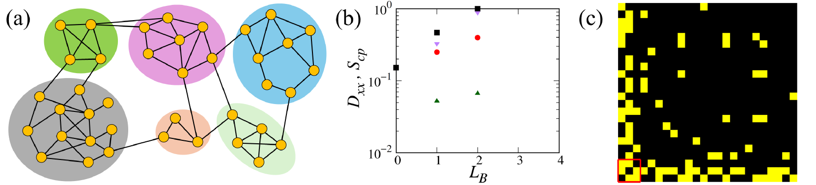
Figure 7: (a) An example of a network with a community structure marked by different background colors. (b) Inside an arbitrary community of the CB network, we plot the connection densities of core-core, core-periphery, and periphery-periphery, along with the core-periphery score, as a function of the boundary level $L_{B}$. The same colors and shapes are used for the densities and the score as in Fig. 6. The core-periphery score $S_{cp}$ reaches its maximum at $L_{B}=2$. (c) The adjacency matrix represents the connections (yellow in the black background) inside the community in panel (b), where nodes are sorted by their LED levels (higher levels toward the left bottom). The nodes inside the red square are the optimal core nodes of this community.

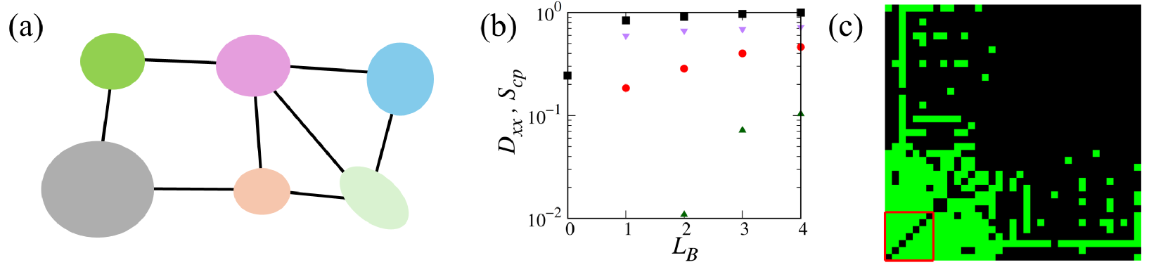
Figure 8: (a) The supernode network is composed of the nodes corresponding to the communities in the network shown in Fig. 7(a). (b) The connection densities of core-core, core-periphery, and periphery-periphery, along with the core-periphery score, as a function of the boundary level $L_{B}$ in the supernode network from the CB network. The same colors and shapes are used for the densities and the score as in Figs. 6 and 7. The core-periphery score $S_{cp}$ reaches its maximum at $L_{B}=4$. (c) The adjacency matrix represents the connections (green in the black background) between the supernodes in panel (b), where nodes are sorted by their LED levels (higher levels toward the left bottom). The supernodes inside the red square are the optimal core nodes of this community.

In the previous subsection, we have found a single core of the network, but as introduced in the first part of Sec. III, more recent studies on the CP emphasize the necessity for the consideration of multiple CP in networks [19, 20, 21, 22]. One hint from the literature is the fact that the mixture of community structures and CP is interchangeably expressed as ‘CP inside communities’ and ‘communities inside CP’ (see Fig. 1.1 of Ref. [17]). In this subsection, we take both viewpoints by applying the LED to the nodes inside each community (the former) and to coarse-grained communities (the latter). For this (literally) divide-and-conquer strategy, we use the Louvain method [46, 47] to systematically obtain community structures.

First, we implement the LED in each community as shown in Fig. 7(a); we treat each community as an individual network by only considering the nodes and edges inside. Again, we take the CB network [37] and detect communities with the Louvain algorithm [46] using the resolution parameter [47] $\gamma=0.5$ in the modularity function [48]. Although the resultant communities can be different for each realization by the algorithm’s stochasticity [49, 50], we obtain $36$ communities in this case. Then, we take each community (except for $8$ communities with the topology of the star graph, where $S_{cp}$ is undefined because $D_{cc}$ is undefined ) and decompose the nodes inside with the LED, by treating the community and connections inside as a network. In contrast to the core-periphery score $S_{cp}\lesssim 0.1$ at the optimal value $L_{B}^{*}$ for the entire network, the mean value of the core-periphery score averaged over all of the communities is $\langle S_{cp}\rangle_{\mathrm{comm}}=0.32(3)$ (the standard deviation in the parenthesis). Therefore, one can see that the community is an appropriate scale to identify a single CP, by lower structural diversity inside. As an illustrative example with a particularly large $S_{cp}$ value, we take a community with the maximum $S_{cp}(L_{B}^{*}=2)=0.882$. Figure 7(b) shows the connection densities and core-periphery score according to the boundary level, as in the entire network in Fig. 6. To visually inspect the actual organization, we plot the community’s adjacency matrix sorted by the nodes’ hierarchy level in Fig. 7(c). In this case, the optimal value $L_{B}^{*}=2$ happens to be the final decomposition stage, which designates the $3$-clique (marked by the red square) as the core. The well-defined single CP inside a community is observed across most communities, and there are extreme CP cases where a single node forms the core (the star-graph structure) as discussed before.

To check the ‘communities inside CP’ side, we take the coarse-grained point of view and treat each community detected by the Louvain algorithm [46, 47] as a new node or a “supernode” for distinction. The supernode network is composed of supernodes and the edges connecting them if there is any connection between the members of each community, as illustrated in Fig. 8(a) compared to Fig. 7(a); multi-edges and self-loops are ignored for simplicity. Then, on this coarse-grained network [52, 53], we apply the same LED process to detect the CP. Figure 8(b) shows the result for the supernode network from the CB network, again in the case of $\gamma=0.5$. The result indicates $L_{B}^{*}\geq 4$ in this case, which assigns the $7$-clique in the super-adjacency matrix depicted in Fig. 8(c). The super-adjacency matrix looks similar to the ideal CP form indeed; the core nodes are fully connected and most periphery nodes are connected to the core nodes. As in the inside-community version of LED, the structural simplification performed by coarse-graining with Louvain communities enables us to find a simple CP. There are communities or supernodes playing a core role in the super-network composed of supernodes. When using the Louvain method, the number of communities varies depending on the resolution parameter $\gamma$, and the nodes comprising each community change for each run even for a single $\gamma$ value due to its stochasticity. However, except for extreme cases where the resolution is very close to $0$ or significantly greater than $1$, results are qualitatively similar to the result obtained in this section.

Finally, we would like to remark on the utility of the hub centrality in this context. The degree as the number of neighbors measures a node’s global significance within the entire network, which is certainly a useful and the most widely used one. However, depending on the purpose of the analysis, comparing the (global) degree values across different focused groups can make deciphering hidden organizational principles even harder, especially in the case of quite heterogeneous degree distributions characterizing real networks [1, 2, 3]. The hub centrality [23, 7] is a tailor-made measure to quantify each node’s relative importance within each focused group composed of the node itself and its neighbors, and it can help us overcome such limitations by standardizing the status of local hubs (recall Fig. 5). Utilizing the hub centrality, the LED assigns standardized levels to local units and identifies the CP based on these levels, and thus, it is versatile across different scales, such as a network, within a community, or a supernode network.

IV Summary and outlook

We have proposed a method to uncover the core-periphery structure of networks through network decomposition centered around local hubs. Compared with other edge or node centralities such as edge betweenness and degree-product, our hub-centrality-product rule ensures the existence of a series of natural cutoffs in the form of a cusp on the giant component size versus the fraction of removed edges. The cusp point, unambiguously defined as the transition point of removed edges with zero versus nonzero hub-centrality product, signals the breaking point of a shell from a backbone. Our local-edge decomposition method repeats this process for each backbone as a brand-new network until we run out of edges to be removed. We have demonstrated the properties and implications of the method with a collaboration network as a representative example, in particular, compared with the celebrated k-core decomposition.

Naturally, the decomposition yields the core-periphery separation and we have introduced a principled way to pinpoint the boundary by the core-periphery score accounting the similarity to the ideal core-periphery structure with respect to the background edge density; in particular, we would like to emphasize again that our local-edge decomposition shines when it is combined with community division, by preparing the groups with appropriate sizes to handle with the decomposition in advance. We believe that the combination leads to the most natural way to extract so-called multiple core-periphery structures [19, 20, 21, 22], and the extension to the coarse-grained communities as supernodes clearly demonstrates the intermingled structure of core-periphery and communities [17]. From the result, we have clearly shown the merit of embracing local hubs in structurally dissecting networks, as in the previously reported effect on dynamical properties [23, 7]. Most of all, we hope that this type of perspective regarding locally important substructures, such as the concept of hidden dependency between nodes from it [54], gets more attention from the network science community.

References

- Newman [2018] M. E. J. Newman, Networks, 2nd ed. (Oxford University Press, Oxford, UK, 2018).
- Barabási [2016] A.-L. Barabási, Network Science (Cambridge University Press, Cambridge, UK, 2016).
- Menczer et al. [2020a] F. Menczer, S. Fortunato, and C. A. Davis, A First Course in Network Science (Cambridge University Press, Cambridge, UK, 2020).
- Dorogovtsev and Mendes [2022] S. N. Dorogovtsev and J. F. F. Mendes, The Nature of Complex Networks (Oxford University Press, Oxford, UK, 2022).
- Albert et al. [2000] R. Albert, H. Jeong, and A.-L. Barabási, Error and attack tolerance of complex networks, Nature 406, 378 (2000).
- Holme et al. [2002] P. Holme, B. J. Kim, C. N. Yoon, and S. K. Han, Attack vulnerability of complex networks, Phys. Rev. E 65, 056109 (2002).
- Jeong and Yu [2022] W. Jeong and U. Yu, Universal behaviour of the growth method and importance of local hubs in cascading failure, J. Complex Netw. 10, cnac028 (2022).
- Pastor-Satorras and Vespignani [2001] R. Pastor-Satorras and A. Vespignani, Epidemic spreading in scale-free networks, Phys. Rev. Lett. 86, 3200 (2001).
- Dorogovtsev et al. [2008] S. N. Dorogovtsev, A. V. Goltsev, and J. F. F. Mendes, Critical phenomena in complex networks, Rev. Mod. Phys. 80, 1275 (2008).
- Liu et al. [2011] Y.-Y. Liu, J.-J. Slotine, and A.-L. Barabási, Controllability of complex networks, Nature 473, 167 (2011).
- Barabási and Albert [1999] A.-L. Barabási and R. Albert, Science 286, 509 (1999).
- Kitsak et al. [2010] M. Kitsak, L. K. Gallos, S. Havlin, F. Liljeros, L. Muchnik, H. E. Stanley, and H. A. Makse, Identification of influential spreaders in complex networks, Nat. phys. 6, 888 (2010).
- Seidman [1983] S. B. Seidman, Network structure and minimum degree, Soc. Netw. 5, 269 (1983).
- Borgatti and Everett [2000] S. P. Borgatti and M. G. Everett, Models of core/periphery structures, Social Networks 21, 375 (2000).
- Holme [2005] P. Holme, Core-periphery organization of complex networks, Phys. Rev. E 72, 046111 (2005).
- Csermely et al. [2013] P. Csermely, A. London, L.-Y. Wu, and B. Uzzi, Structure and dynamics of core/periphery networks, J. Complex Netw. 1, 93 (2013).
- Rombach et al. [2017] P. Rombach, M. A. Porter, J. H. Fowler, and P. J. Mucha, Core-periphery structure in networks (revisited), SIAM Review 59, 619 (2017).
- Tang et al. [2019] W. Tang, L. Zhao, W. Liu, Y. Liu, and B. Yan, Recent advance on detecting core-periphery structure: A survey, CCF Trans. Pervasive Comput. Interact. 1, 175 (2019).
- Kojaku and Masuda [2017] S. Kojaku and N. Masuda, Finding multiple core-periphery pairs in networks, Phys. Rev. E 96, 052313 (2017).
- Kojaku and Masuda [2018] S. Kojaku and N. Masuda, Core-periphery structure requires something else in the network, New J. Phys. 20, 043012 (2018).
- Yang et al. [2018] J. Yang, M. Zhang, K. N. Shen, X. Ju, and X. Guo, Structural correlation between communities and core-periphery structures in soc. netw.: Evidence from twitter data, Expert Syst. Appl. 111, 91 (2018), big Data Analytics for Business Intelligence.
- Gallagher et al. [2021] R. J. Gallagher, J.-G. Young, and B. F. Welles, A clarified typology of core-periphery structure in networks, Sci. Adv. 7, eabc9800 (2021).
- Jeong and Yu [2021] W. Jeong and U. Yu, Critical phenomena and strategy ordering with hub centrality approach in the aspiration-based coordination game, Chaos 31, 093114 (2021).
- Valdez et al. [2020] L. D. Valdez, L. Shekhtman, C. E. La Rocca, X. Zhang, S. V. Buldyrev, P. A. Trunfio, L. A. Braunstein, and S. Havlin, Cascading failures in complex networks, J. Complex Netw. 8, cnaa013 (2020).
- Buldyrev et al. [2010] S. V. Buldyrev, R. Parshani, G. Paul, H. E. Stanley, and S. Havlin, Catastrophic cascade of failures in interdependent networks, Nature 464, 1025 (2010).
- Cohen et al. [2003] R. Cohen, S. Havlin, and D. ben-Avraham, Efficient immunization strategies for computer networks and populations, Phys. Rev. Lett. 91, 247901 (2003).
- Gómez-Gardeñes et al. [2007] J. Gómez-Gardeñes, M. Campillo, L. M. Floría, and Y. Moreno, Dynamical organization of cooperation in complex topologies, Phys. Rev. Lett. 98, 108103 (2007).
- Porter et al. [2009] M. A. Porter, J.-P. Onnela, and P. J. Mucha, Communities in networks, Not. Am. Math. Soc. 56, 1082 (2009).
- Fortunato [2010] S. Fortunato, Community detection in graphs, Phys. Rep. 486, 75 (2010).
- Fortunato and Newman [2022] S. Fortunato and M. E. J. Newman, 20 years of network community detection, Nature Physics 18, 848 (2022).
- Wu and Holme [2011] Z.-X. Wu and P. Holme, Onion structure and network robustness, Phys. Rev. E 84, 026106 (2011).
- Yang et al. [2017] Y. Yang, T. Nishikawa, and A. E. Motter, Small vulnerable sets determine large network cascades in power grids, Science 358, eaan3184 (2017), https://www.science.org/doi/pdf/10.1126/science.aan3184 .
- Kempe et al. [2003] D. Kempe, J. Kleinberg, and É. Tardos, Maximizing the spread of influence through a social network, in Proceedings of the Ninth ACM SIGKDD International Conference on Knowledge Discovery and Data Mining, KDD ’03 (Association for Computing Machinery, New York, NY, USA, 2003) pp. 137–146.
- Freeman [1977] L. C. Freeman, A set of measures of centrality based on betweenness, Sociometry 40, 35 (1977).
- Note [1] Another side effect of such recalculation is that the whole process would depend heavily on the order of removed edges with the same value of , which leads to much more complicated situations in practice that requires ensemble average over multiple realizations.
- Note [2] We suggest using the heap queue structure in numerical simulations for this.
- Batagelj and Mrvar [2006] V. Batagelj and A. Mrvar, Pajek datasets, http://vlado.fmf.uni-lj.si/pub/networks/data (2006).
- Leskovec et al. [2009] J. Leskovec, K. J. Lang, A. Dasgupta, and M. W. Mahoney, Community structure in large networks: Natural cluster sizes and the absence of large well-defined clusters, Internet Math. 6, 29 (2009).
- Cho et al. [2011] E. Cho, S. A. Myers, and J. Leskovec, Friendship and mobility: user movement in location-based soc. netw., in in Proc. 17th ACM SIGKDD Int. Conf. Knowl. Disc. Data Min. (2011) pp. 1082––1090.
- Fellbaum [1998] C. Fellbaum, ed., WordNet: an Electronic Lexical Database (MIT Press, 1998).
- Note [3] One can imagine a following (extreme) case: assume a node with connected to a number of other nodes, all of which have and are connected to very large and dense clique-like subnetworks on the other side than the original node itself. In that case, by the elimination of the neighboring nodes, the original node will be isolated. This effect is reflected in the actual appearance of in Fig. 2(d), but actually it is quite rare (usually less than of nodes in our empirical networks).
- Lee et al. [2014] S. H. Lee, M. Cucuringu, and M. A. Porter, Density-based and transport-based core-periphery structures in networks, Phys. Rev. E 89, 032810 (2014).
- Cucuringu et al. [2016] M. Cucuringu, P. Rombach, S. H. Lee, and M. A. Porter, Detection of core-periphery structure in networks using spectral methods and geodesic paths, European Journal of Applied Mathematics 27, 846–887 (2016).
- Menczer et al. [2020b] F. Menczer, S. Fortunato, and C. A. Davis, A first course in network science (Cambridge University Press, Cambridge, England, 2020).
- Note [4] In contrast to our decomposition method from the hub centrality, the degree values are changed in real-time and instantly reflected in the node-removal process.
- Blondel et al. [2008] V. D. Blondel, J.-L. Guillaume, R. Lambiotte, and E. Lefebvre, Fast unfolding of communities in large networks, J. Stat. Mech. 2008, P10008 (2008).
- Reichardt and Bornholdt [2006] J. Reichardt and S. Bornholdt, Statistical mechanics of community detection, Phys. Rev. E 74, 016110 (2006).
- Newman and Girvan [2004] M. E. J. Newman and M. Girvan, Finding and evaluating community structure in networks, Phys. Rev. E 69, 026113 (2004).
- Kim and Lee [2019] H. Kim and S. H. Lee, Relational flexibility of network elements based on inconsistent community detection, Phys. Rev. E 100, 022311 (2019).
- Lee et al. [2021a] D. Lee, S. H. Lee, B. J. Kim, and H. Kim, Consistency landscape of network communities, Phys. Rev. E 103, 052306 (2021a).
- Note [5] Note that, in a sense, the star graph is the perfect CP and it should strongly positively contribute to .
- Itzkovitz et al. [2005] S. Itzkovitz, R. Levitt, N. Kashtan, R. Milo, M. Itzkovitz, and U. Alon, Coarse-graining and self-dissimilarity of complex networks, Phys. Rev. E 71, 016127 (2005).
- Song et al. [2005] C. Song, S. Havlin, and H. A. Makse, Self-similarity of complex networks, Nature 433, 392 (2005).
- Lee et al. [2021b] M. J. Lee, E. Lee, B. Lee, H. Jeong, D.-S. Lee, and S. H. Lee, Uncovering hidden dependency in weighted networks via information entropy, Phys. Rev. Res. 3, 043136 (2021b).