qLUE: A Quantum Clustering Algorithm for Multi-Dimensional Datasets
Abstract
Clustering algorithms are at the basis of several technological applications, and are fueling the development of rapidly evolving fields such as machine learning. In the recent past, however, it has become apparent that they face challenges stemming from datasets that span more spatial dimensions. In fact, the best-performing clustering algorithms scale linearly in the number of points, but quadratically with respect to the local density of points. In this work, we introduce qLUE, a quantum clustering algorithm that scales linearly in both the number of points and their density. qLUE is inspired by CLUE, an algorithm developed to address the challenging time and memory budgets of Event Reconstruction (ER) in future High-Energy Physics experiments. As such, qLUE marries decades of development with the quadratic speedup provided by quantum computers. We numerically test qLUE in several scenarios, demonstrating its effectiveness and proving it to be a promising route to handle complex data analysis tasks – especially in high-dimensional datasets with high densities of points. The code we used for these simulations is available at Ref. [1]
1 Introduction
Clustering is a data analysis technique that is crucial in several fields, owing to its ability to uncover hidden patterns and structures within large datasets. It is essential for simplifying complex data, improving data organization, and enhancing decision-making processes [2, 3, 4, 5]. For instance, clustering has been applied in marketing [6, 7], where it helps segment customers for targeted advertising [8], and in biology, for classifying genes and identifying protein interactions [9, 10, 11, 12]. In the realm of computer science and artificial intelligence, it is invaluable for image [13] and speech recognition [14, 15], as well as recommendation systems [16, 17] that personalize content for users. Finally, clustering techniques are pivotal for Event Reconstruction (ER), where data points that originated from the same “event” must be collected together. In High-Energy Physics, for instance, clustering algorithms reconstruct the trajectories of subatomic particles in collider experiments. It is expected that the endcap high granularity calorimeter (HGCAL) [18] being built for the CMS detector at the High Luminosity Large Hadron Collider will provide extremely large volumes of data that must be tackled by new generations of clustering algorithms such as CLUE. The discovery of the Higgs boson [19], awarded the Nobel prize in 2012, was made possible by such algorithms.
ER enables the interpretation of data obtained from particle collision events, including those occurring at the Large Hadron Collider (LHC) at CERN. Several clustering algorithms like DBScan, K-Means, and Hierarchical Clustering among others [20, 21, 22] can be employed for ER. Our work is based on CERN’s CLUstering of Energy (CLUE) algorithm [23], which is adopted by the CMS collaboration [24, 25, 26]. It is designed for the future HGCAL detector due to the limitations of the currently employed algorithms. Despite these limitations, such algorithms are already at the basis of several discoveries, such as the doubly charged tetraquark [27], the observation of four-top quark production in proton-proton collisions [24] and the study of rare B meson decays to two muons [25].
The efficiency of clustering algorithms, as illustrated by the CLUE algorithm [23], is crucial for handling extensive datasets. Initially designed for two-dimensional datasets, CLUE reduces the search complexity from to through the use of local density and a tiling procedure, where () represents the (average) number of points (per tile).
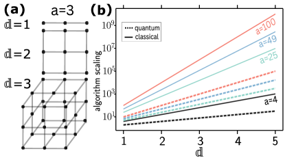
In the context of CLUE, where data sets are limited to two dimensions, is small, making this approach to ER particularly effective. However, as the dimensionality of the dataset is incremented, the value of generally increases exponentially. This is highlighted by Fig. 1(a), where for a -dimensional lattice with points per edge, follows the relation . This is a serious challenge to CLUE and classical clustering algorithms in general.
A first step towards extending CLUE to more dimensions is done by 3D-CLUE [23, 29]. In this work, data points from different layers of detectors are first projected onto a single surface, where clustering is then performed. However, this projection from the original dataset to a surface comes at the cost of a slower algorithm since becomes effectively larger. The solid lines in Fig. 1(b) show the increase in average points per tile in -dimensional datasets made of the lattices in panel (a). While the improved performance of 3D-CLUE in ER tasks [23, 29] justifies the increased computational overhead, extending this enhancement to higher dimensions and larger datasets is challenging. Finding practical approaches to deal with datasets where is large is therefore extremely important, not only for ER tasks but also in other fields such as gene analysis [30] and market segmentation in business [31].
Quantum computers provide a route to mitigate the complexity blowup arising from higher dimensional datasets. Ref. [32] addresses the task of jet clustering in High-Energy Physics, while Ref. [33] targets spectral clustering, which itself uses the efficient quantum analog of -means clustering [34]. Other approaches include quantum -medians clustering [35] and a quantum algorithm for density peak clustering [36].
In this work we develop qLUE, a CLUE-inspired quantum algorithm. Similarly to other quantum algorithms [37, 38], qLUE leverages the advantage provided by Grover Search [28]. A comparison of classical and quantum (Grover) runtimes is presented in Fig. 1(b), where the solid [dashed] lines refer to the classical [quantum ] scaling. As can be seen, the complexity advantage that Grover search provides can be substantial, particularly for large values of or .
Overall, we find that qLUE performs well in a wide range of scenarios. With ER-inspired datasets as a specific example, we demonstrate that clusters are correctly reconstructed in typical experimental settings. Similar to other quantum approaches to clustering that rely on Grover Search [35, 39], qLUE also showcases a quadratic speedup compared to classical algorithms. The specific advantages of qLUE are its CLUE-inspired approach to cluster reconstruction (which demonstrated to be extremely successful [24, 40, 25]), and its consequent seamless integration with the classical framework currently employed by the CMS collaboration [23, 29, 41].
This paper is structured as follows. In Sec. 2, we describe our algorithm qLUE. Specifically, we provide a general overview of its subroutines – namely the Compute Local Density, Find Nearest Higher, and the Find Seeds, Outliers and Assign Clusters steps. We describe the results of our simulated version of qLUE on a classical computer in Sec. 3. In more detail, we explain the scoring metrics we use to quantify our results, and describe qLUE performance when the dataset is subject to noise and different clusters overlap. Conclusions and outlook are finally presented in Sec. 4.
2 qLUE
qLUE is a quantum adaptation of CERN’s CLUE and 3D-CLUE algorithms [23, 29], that is specifically developed for ER, yet it is suitable to work with any (high dimensional) dataset. The main advantage of qLUE stems from employing Grover’s algorithm, which provides a quadratic speedup for the Unstructured Search Problem [28]. While qLUE is designed to work in arbitrary dimensions, for clarity we restrict ourselves to . This simplifies the following discussions and allows us to simulate qLUE with meaningful datasets on a classical computer. Generalizations to higher dimensions can be done following the steps outlined below. Furthermore, to provide a better connection with CLUE and 3D-CLUE, we employ a similar notation.
In Sec. 2.1, we offer an overview of the algorithm and its different subroutines. Sec. 2.2 is dedicated to the first subroutine of qLUE, namely, calculating the Local Density. We then explain how to determine the Nearest Highers (), Seeds, and Outliers in Sec. 2.3. Finally, Sec. 2.4 delves into the conclusive Cluster Assignment subroutine, where the points in the dataset are effectively heirarchically clustered.
2.1 Overview and Setting
As for CLUE and 3D-CLUE [23, 29], we consider a dataset with spatial coordinates and an energy for every point. Similar datasets can also be found in medical image analysis and segmentation [42, 43], in the analysis of asteroid reflectance spectra and hyperspectral astronomical imagery in astrophysics [44, 45, 46] and in gene analysis in bioinformatics [30, 47].
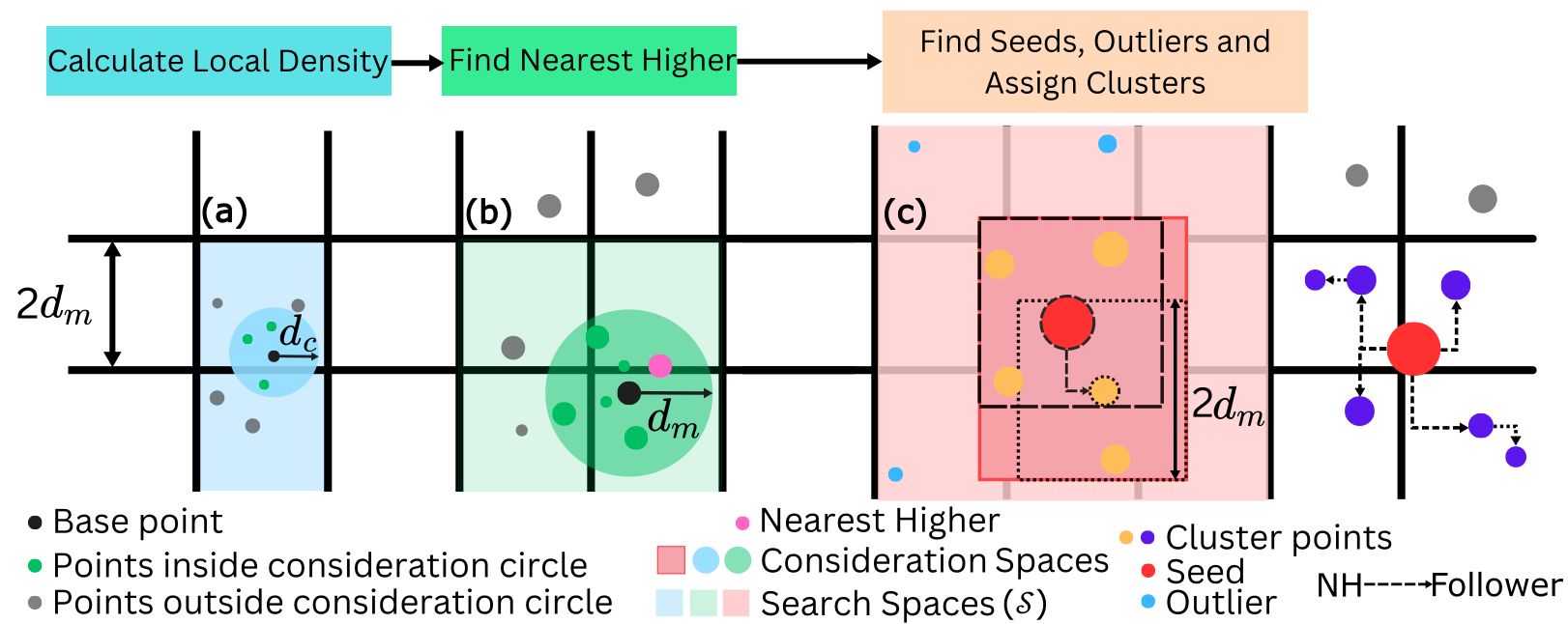
In dimensions, the spatial coordinates for point are , that are promptly generalized for larger values of . Both CLUE and qLUE first perform tiling over the dataset to reduce the search and therefore enhance the efficiency of the algorithm. Tiling is the process of partitioning the dataset into a grid of rectangular tiles , where is the tile index (see Fig. 2). Therefore, our input dataset comprises of point and tile indices and , respectively, the coordinates , and a parameter associated to each point. Following CLUE’s notation, we call the energy, yet this should be considered as a label that can be employed to improve the clustering quality for any given dataset. The tiling procedure of qLUE and CLUE enables searching only over Search Spaces marked by the tiles in green in Fig. 2(a) as opposed to the full dataset. In case of CLUE, this allowed for an improvement in scaling from to . The scaling of qLUE is investigated below.
In this work, we employ a qRAM to store and access data, which is an essential building block for quantum computers. Following Ref. [48], we therefore assume that we can efficiently prepare the state
| (1) |
where is the data associated with a given index , e.g. the point in the database. For convenience, here and throughout this paper we do not explicitly write the normalization factors of quantum states.
The qLUE algorithm consists of the following steps:
Local Density: The first step is to calculate the local density of all points [e.g, black point in Fig. 2(a)] that is defined by
| (2) |
and it is indicative of the energy in a neighbourhood of point . As can be seen from Eq. (2) and Fig. 2(a), is a weighted sum over the energies of all points whose distance from the base point is within a user-specified critical radius that characterizes the consideration circle for the Local Density computation subroutine (light blue circle in the figure).
As such, is the energy of the point which is away from point . The choice of weight for in the definition of in Eq. (2) is empirically found to yield better performances for CLUE [23].
Find Nearest Higher: After calculating the local densities, we determine the nearest highers. The Nearest Higher of a point is the point nearest to with a higher local density . As better explained in Sec. 2.4, the Nearest Higher are used to heirarchically cluster points together in the Cluster Assignment process at the end of qLUE. In Fig. 2(b), the Nearest Higher of the base point (black point) is the pink point.
Find Seeds, Outliers and Assign Clusters: As schematically represented in Fig. 2(c), seeds (red points) are the points whose distance from their Nearest Higher and whose local density are lower bounded by user defined thresholds. Outliers (blue points) are the points whose distance from Nearest Higher is similarly lower bounded but whose Local Density has an upper threshold. As such a point is
| a seed if | (3a) | |||
| an outlier if | (3b) | |||
Here, is the Outlier Delta Factor that determines the upper bound on the allowed local density for outliers. Furthermore, is the critical density threshold – the lowest local density a point can have to be classified as a seed. Both and are user-specified and can be varied to enhance the quality of the output. Seeds are generally located in areas of high energy density, and will be employed as starting points to build clusters. Outliers are points that are likely to be noise in the dataset and are therefore discarded.
Once seeds and outliers are determined, the clusters are constructed. From the seeds, we iteratively combine “followers”. If point is the Nearest Higher of point , then point is termed as ’s follower. The follower of a point is most likely generated by the same process as the point itself (in the context of ER, by the same particle), and as such shall be included in the same cluster. In Fig. 2(c), the orange and purple points form two different clusters, and the followers of the points in the purple one are indicated by arrows.
2.2 Local Density Computation
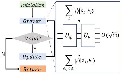
In this section, we describe the subroutine (schematically represented in Fig. 3) that computes the Local Density of the point , as defined in Eq. (2). To perform the computation, all points whose distance from point is smaller than the threshold need to be determined from the search space . This search space is the smallest set of tiles required to cover the consideration circle. In Fig. 2(a), is highlighted in light blue.
We shall refer to as the local dataset that, as explained above, can be efficiently prepared with the qRAM [48]. To do so, we only require determining the tiles that are in the search space, which can be done efficiently classically [23]. The initial state of this subroutine, after being prepared via the qRAM, is therefore
| (4) |
where the index is unique for each point in . indicate all indices within tile [either of the light blue squares in Fig. 2(a)]. Ancillary qubits, omitted for clarity in Eq. (4), are employed within the Grover search (for more information, see App. A).
At this stage, we must find the points [green dots in Fig. 2(a)] that are within a radius of from the base point [black point in Fig. 2(a)]. As shown in Fig. 3, we perform Grover Search to prepare [49]
| (5) |
Here, the first register of the Grover output contains all points characterized by indices such that . As shown in the inset of the figure, the Grover Search consists of repetitions (where is the number of points in ) of the and operators. is the diffusion operator and is the unitary associated with the oracle of Grover Search [28]. Further details regarding Grover Search and the unitaries we use for our algorithm can be found in App. A.
When the algorithm is run, measurement either yields a point that satisfies this distance condition, or (if there are no valid indices left) an index that does not satisfy this condition. This is verified by the grey “Valid?” diamond in Fig. 3. The branched logic following this block ensures that the algorithm loops until all the required points are returned by the algorithm in the “Return” block.
Once we have obtained all indices of points satisfying the distance condition (), we perform the summation in Eq. (2). This is computed and stored in the original dataset for each point. The database is now updated using qRAM with local density values for all points where the point in the database has the corresponding computed local density .
The scaling of the subroutine that determines the local density of a single point is given by the number of points in the blue consideration circle in Fig. 2(a) such that . If we say this number is , runs are required. This is therefore a algorithm as opposed to the classical iterative algorithm for the Unstructured Search Problem.
As a final remark, we highlight that it is in principle possible to design a unitary that computes the Local Density directly and stores the output in a quantum register. This unitary would remove the requirement of finding individually the indices such that , thus removing the overhead of in . However, designing this circuit is non-trivial and its depth may be large. This is therefore left for future investigations.
2.3 Find Nearest Higher
Here, we describe qLUE’s subroutine for finding the Nearest Highers () introduced in Sec. 2.1. As a reminder, is the nearest point to the base point whose local density is more than the local density of the base point, see Eq. (3a).
Similar to the initialization carried out for the Local Density Computation step, we use qRAM to initialize the quantum state
| (6) |
Here, the indices are within the tiles , as in Eq. (4), and is the considered search space, schematically represented by the light green box in Fig. 2(b). This search space is determined from as opposed to , which is the user-defined threshold that is set to be . Note that the energy , employed for determining the densities in Sec. 2.2, is hereon not required.
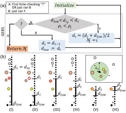
To find the Nearest Higher, we use a Grover-Enhanced Binary Search (GEBS) where each search step is enhanced by Grover’s algorithm. The output of every Grover run,
| (7) |
is a superposition over all points whose distance from the base point lies between the thresholds and . Furthermore, their local density should be higher than that of the base . At each step, and are updated based on whether a point satisfying the conditions in the grey diamond of Fig. 4(a) is found. Ancilla registers are used here as detailed in App. A.
To better understand the algorithm, we provide a step-by-step walkthrough of the example in Fig. 4(b). The search space is schematically represented by the inset in the right hand side, where each dot represents a point with a size that is proportional to its local density. The consideration circle (light green, dotted border) highlights all points within a radius . In this work, we set the outlier delta factor to . The consideration circle in the inset corresponds to and , shown in step (I). In the main panel, vertical lines refers to the steps (I-VI) of GEBS that are reported below, and schematically represent the distances of all points (coloured dots) from the base point (black one at the bottom).
GEBS starts with the higher threshold set as and the lower threshold as shown in vertical line (I) of Fig. 4(b). Following the probabilistic nature of quantum mechanics, assume that the point with a red border indexed is found after measuring the output of the Grover Search in Eq. (7). This triggers the updates in the branch in the diagram of Fig. 4(a), such that we assign and update . The point indexed is then removed from the search space, as can be seen in (II). Now, since no point satisfies the conditions in the diamond of the flow diagram [see (II)] and was just set to , the branch is carried out. This updates the thresholds and for the next iteration of the algorithm, see (III).
Now, assume that the new point with a red border is found [step (III)]. Updates in the branch of Fig. 4(a) are carried out again with a new index and the search region is reduced to contain a single point. In the next step (IV), that point (yellow) is found and, for the third and last time, the nearest higher and the thresholds are triggered according to the branch. Next, since no point is found in (V), qLUE executes the updates in the branch of the diagram. In the last iteration (VI), no points satisfy the desired conditions. The parameter was just set to , i.e, the subroutine just ran which means that the branch is now executed and is returned.
The runtime complexity of the GEBS procedure, with points in the search space , is as opposed to classically. The term is due to the binary search procedure and depends on the size of the quantum register used to encode the distance. Specifically, for a chosen precision used for the positions of the points in the datasets, .
2.4 Find Seeds, Outliers, and Assign Clusters
Once the Nearest Highers are determined for all points in the dataset, Seeds and Outliers are found via another Grover Search over all points in the dataset. As per the definition in Eq. (3a), Seeds [red points in Fig. 2(c)] are the points with highest local density within a neighbourhood. Outliers [blue points in Fig. 2(c)] are mathematically described by Eq. (3b), are most likely noise, and therefore do not belong to any cluster.
Similar to the previous subroutines, the quantum registers for these procedures are initialized via qRAM. Seeds and outliers are then determined based on the corresponding conditions via Grover Search. Two quantum registers, the first marking whether a point is an outlier and the second to store the seed number – which is also the cluster number – are added to the quantum database.
The final subroutine of qLUE is the assignment of points to clusters. At this stage, outliers have been removed from the input dataset, as they have been already identified. The algorithm flow is the same as that of the Local Density step in Fig. 3. For a chosen seed , we define to be the set containing the indices of all points determined to be in the associated cluster at the end of this subroutine. To assign points to , we follow a procedure similar to that of the Local Density step in Fig. 3. In the “Initialize” step, is initialized to and the quantum registers are initialized via qRAM to the state
| (8a) | |||
| (8b) | |||
In the “Grover” block, we search over a superposition of points in the dataset which we call the Dynamic Search Space (DSS). The DSS differs from the search space in the Local Density step as it is dynamic. This is because it depends on the points in , which are updated at each iteration. In Fig. 2(c), for instance, the red seed and the orange point both with black borders are the elements of the current . To find the DSS, a square window of edge is first opened for every point in (in the figure, the squares with the same border style as the corresponding points). A rectangular region (red box) is then obtained by finding the axis-aligned minimum bounding box for these windows. The set of tiles covered partially or fully by this minimum bounding box is the DSS. For example, in Fig. 2(c), it comprises the tiles highlighted in light red.
With a similar procedure as for the Local Density subroutine, the “Grover” block now systematically identifies all followers of all points within set . Here, in the “Update” step in Fig. 3, as the point found by the “Grover” block has passed the “Valid” condition, it is appended to . Once no more points are found, the “Return” block yields , following the same flow as the Local Density computation subroutine.
The complexity of the Cluster Assignment step is similar to the one of the Local Density Computation subroutine. The quantum advantage stems from the quadratic speedup provided by the Grover algorithm, which allows determining the follower faster if compared to CLUE. If there are points in a cluster and points in the corresponding DSS, the classical complexity of the Cluster Assignment step is , while the quantum algorithm has a runtime of .
3 Results
In this section, we test qLUE in multiple scenarios, each designed to investigate its performance for different settings. In Sec. 3.1, we introduce the scoring metrics used for our analysis. In Sec. 3.2, we describe the performance of the algorithm applied on a single cluster in a uniform noisy environment. In Sec. 3.3, we study the performance on overlapping clusters. Finally, in Sec. 3.4, we study the performance of qLUE on non-centroidal clusters with and without an energy profile.
3.1 Scoring metrics: Homogeneity and Completeness scores
To weigh more energetic points such as seeds higher than the others, we use modified, energy-aware versions [51] of the Homogeneity () and Completeness () scores [52]. These metrics are defined in terms of the predicted cluster labels obtained from qLUE, and the true cluster labels of the generated dataset. and are based on the energy aware [51] mutual information , the Shannon entropy , and the joint Shannon entropy [53]:
| (9a) | |||
| (9b) | |||
| (9c) | |||
| (9d) | |||
| (9e) | |||
As discussed in [51], is the energy aggregated over all points that qLUE classifies into cluster . is the energy aggregated over all points in cluster in the true dataset. is the sum of energies of all points in cluster in the true dataset that are also assigned to cluster by qLUE. is the accumulated energy of all points in the dataset. We remark that for unit energies, Eqs. (9) reduce to the more common form presented in Ref. [52].
qLUE applied to an input dataset yields homogeneity if all of the predicted clusters only contain data points that are members of a single true cluster. On the other hand, is obtained if all the data points that are members of a given true cluster are elements of the same reconstructed cluster. Therefore, these metrics are better suited to different scenarios. The impacts of noise and cluster overlap investigated in Secs. 3.2 and 3.3 are better captured by . Indeed, if qLUE incorrectly classifies noise points into predicted clusters, is unaffected. On the other hand, shall be employed when studying non-centroidal clusters in Sec. 3.4, since if one true cluster is divided by qLUE into many sub-clusters.
3.2 Noise
Here, we study the performance of qLUE for a single cluster in a noisy environment. We vary the number of noise points sampled from a uniform distribution over a square region of fixed size. A cluster of points with coordinates is sampled from the multivariate Gaussian distribution
| (10) |
where is the mean of the distribution (set to in our case) and the covariance matrix. Here, we choose , with being the identity matrix and a positive real number.
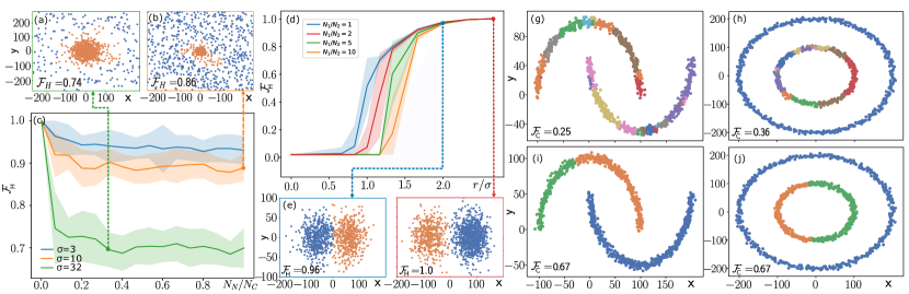
Examples of the generated clusters (in orange) and noise (in blue) are given in Fig. 5(a-b) for at and at , respectively. The energy assigned to each point in the cluster is given by [see Eq. (10)] with . The energy of each noise point is randomly sampled between zero and one. This choice resembles the typical scenarios in ER tasks which CLUE [23] was designed for.
In Fig. 5(c), we show the variation of homogeneity score with respect to the ratio . We employ the values of reported in the legend, that are associated to different colours in the plot. As can be seen, the clustering performance is inversely proportional to both and . When these parameters are small, the typical distance between cluster points is much smaller than that between noise points, and approaches unity. With a higher chance of labeling noisy points as within the cluster, however, is lowered. As such, the degrading of is proportional to the probability of a noise point being in the cluster region, which increases with both and .
3.3 Overlap
Here, we consider the case of two circular clusters with and points respectively, each sampled from the multivariate Gaussian distribution in Eq. (10) and with . The energy profile is determined by for coordinates . The centers and (two instances of ) are chosen to be and , respectively, such that the distance between the cluster centers is .
In Fig. 5(d), we study the variation of homogeneity score as a function of for several values of . The computed clusters for at and at are shown in panels (e) and (f), respectively, to showcase the typical scenarios considered here.
For all , is zero for low (high overlap). There is then a region where increases with and then saturates at unity for high (little to no overlap). When the two clusters are too nearby, i.e., , they are in fact indistinguishable and qLUE labels all points together. Increasing the ratio makes the clusters move away from each other and thus qLUE can discern them. Importantly, large values of are already attained when the clusters still have a significant overlap. In this scenario, employing the energy labels and the energy density considerably contributes to assigning the points to the right cluster. In fact, the nearest higher points are more likely to connect the points near or on the decision boundary with the more energetic core, thus separating the clusters better.
The performance of qLUE is also affected by the ratio . When one cluster contains more points than the other, it is more likely to “capture” points from the smaller. The resulting loss in homogeneity score for low ratios is evident from Fig. 5(d), where it can be seen that clusters of similar sizes are better distinguished from each other.
3.4 Non-centroidal Clusters
Finally, we study the performance of qLUE on non-centroidal clusters. For this purpose, we use the Moons and Circles datasets in Fig. 5(g-j), generated using [50]. Two settings are considered - one where a uniform energy profile is applied over the points [panels (g-h)] and one where a linear gradient energy profile is employed [panels (i-j)].
In the latter case, for each cluster we assign the highest value of the energy to a single point and lower the energies of all other points proportionally to their coordinate. In the case of the moon dataset, for the upper moon (so the top point of the upper moon has the maximum energy in the cluster) and for the lower moon (so the bottom point has the highest energy in the cluster). For the circles, for the inner circle and for the outer one.
Since these datasets have no noise and are well separated, is always one and we employ to characterize the performance of qLUE. As in Fig. 5(g-h) the energy profile is uniform, and several points satisfy the seed condition. Therefore, qLUE groups each circle into several clusters, such that we obtain limited values for . On the contrary, cases with an energy profile assigned [Fig. 5(i-j)] results in less seeds that are better recognized by qLUE, and the completeness score is considerably enhanced.
4 Conclusion and Outlook
We introduced qLUE, a novel quantum clustering algorithm designed to address the computational challenges associated with high-dimensional datasets. The significance of qLUE lies in its potential to efficiently cluster data leveraging quantum computing, mitigating the escalating computational complexity encountered by classical algorithms as dimensions increase. The algorithm’s ability to navigate high-dimensional spaces is particularly promising when the density of points is very large, such that local searches become too demanding for classical computers. Therefore, qLUE will be beneficial in multiple scenarios, ranging from quantum-enhanced machine learning [54, 55] to complex data analysis tasks [56].
According to our numerical results, qLUE works well and its performance is significantly enhanced when an energy profile is assigned. Specifically, we study qLUE in noisy environments, on overlapping clusters, and on non-centroidal datasets that are commonly used to benchmark clustering algorithms [57, 58]. In scenarios that are typically encountered in ER tasks, qLUE correctly reconstructs the true clusters to a high level of accuracy. On the other hand, an energy profile can significantly boost qLUE performance in the case of non-centroidal clusters. Our numerical results, backed up by the well-studied CLUE and by the quadratic speedup stemming from Grover search, make qLUE a promising candidate for addressing high-dimensional clustering problems [32, 33, 36].
As a first outlook, we identify the implementation of qLUE on NISQ hardware [59, 60, 61, 62, 63, 64, 65]. This requires a comprehensive consideration of real device constraints. Aspects such as circuit optimization [66], and the impact of noise will be critical and must be carefully addressed. Second, it is possible to improve the scaling of qLUE by devising a unitary that mitigates the need for repeating Grover’s algorithm and thereby eliminating the factors of , , and in the scaling of the subroutines outlined in Secs. 2.2, 2.3 and 2.4 respectively. Finally, it is worth investigating variations of qLUE that improve the quality of clustering in different scenarios. For instance, one can devise more sophisticated criteria for the Nearest Higher or Local Density computation steps. One can also improve performance by performing exhaustive hyperparameter searches or via hyperparameter optimization algorithms [67].
Acknowledgements
We thank the CERN Quantum Initiative, Fabio Fracas for creating the fertile ground for starting this project and Andrew J. Jena as well as Priyanka Mukhopadhyay for theoretical support. WR acknowledges the Wolfgang Gentner Programme of the German Federal Ministry of Education and Research (grant no. 13E18CHA). LD acknowledges the EPSRC quantum career development grant EP/W028301/1. DG and MM acknowledge the NTT PHI Lab for funding. Research at IQC is further supported by the Government of Canada through Innovation, Science and Economic Development Canada (ISED). Research at Perimeter Institute is supported in part by the Government of Canada through ISED and by the Province of Ontario through the Ministry of Colleges and Universities.
Appendix
Appendix A Grover’s Algorithm
Grover’s algorithm is a quantum algorithm to solve the Unstructured Search Problem. From a superposition of all states to be searched over, Grover’s algorithm involves successive applications of two operators and to ensure that the measurement result at the end of the algorithm gives the search output with high probability. We use this algorithm extensively in our work. The inset of Fig. 3 describes the flow of this algorithm for our Local Density computation step. For points, this involves successive applications of the operators
| (11a) | ||||
| (11b) | ||||
Here, when the current point satisfies a desired condition (e.g in the context of Local Density Computation, it lies in the critical radius ). If this condition is not satisfied, .
To implement the operators in Eqs. (11), we require A(dd) and M(ultiply) circuits. We use the ones introduced in Ref. [68], which perform the following operations
| (12a) | ||||
| (12b) | ||||
For the local density step, the quantum circuit to implement the search function is given in Fig. 6. The overall idea is to compute the Euclidean distance between every input point and the base point and check if this distance is higher than . The qubit stores the output of this computation. The gates are gates which are on the sign qubit and act as the identity on every other qubit, such that . These are used such that the first and second levels of Add gates compute into and respectively. The multiply gates then set the states to taking and as inputs. An gate next acts on and to set to . The gate is a subcircuit of the addition circuit that finally computes the sign of and stores it in . Thus, [with as in Eq. (11b)] for the Local Density computation step.

For the Nearest Higher Procedure, a similar circuit can be used with additional registers for the Local Density and for the critical density threshold . is replaced by and the signs of and are additionally computed in order to find only the points that lie between and and satisfy the threshold. These signs can be combined with the Toffoli gate to compute the required function
For Seeds and Outliers, the condition is similar to that in the Nearest Higher (GEBS) procedure in that the distance criterion is only a lower bound as opposed to a window. The GEBS blackbox without the upper distance bound computation can be used.
For the Cluster Assignment step, the operator needs to check if the Nearest Higher index of the points over which Grover Search is carried out lies within . The operator for this can be generated using and gates. gates map to and act as the identity on all the other elements of the computational basis. Let us consider a simple example where the dynamic search space DSS has points indexed from to in binary. So, the Nearest Higher index will always be in this range. If consists of indices and , we would use as defined in Fig. 7. This flips the phase of and in the input superposition as required (following Eq. (12b)). As shown in Fig. 7, operators for each index can be sequentially applied to check for multiple indices in .
References
- [1] Dhruv Gopalakrishnan et al. “QLUE-algo/qlue: frontiers-paper” Zenodo, 2024 DOI: 10.5281/zenodo.12655189
- [2] Zuguang Gu and Daniel Hübschmann “SimplifyEnrichment: A Bioconductor Package for Clustering and Visualizing Functional Enrichment Results” In Genomics, Proteomics and Bioinformatics 21.1, 2022, pp. 190–202 DOI: 10.1016/j.gpb.2022.04.008
- [3] Jelili Oyelade et al. “Data Clustering: Algorithms and Its Applications” In 2019 19th International Conference on Computational Science and Its Applications (ICCSA), 2019, pp. 71–81 DOI: 10.1109/ICCSA.2019.000-1
- [4] Tong Wu, Xinwang Liu, Jindong Qin and Francisco Herrera “Balance Dynamic Clustering Analysis and Consensus Reaching Process With Consensus Evolution Networks in Large-Scale Group Decision Making” In IEEE Transactions on Fuzzy Systems 29.2, 2021, pp. 357–371 DOI: 10.1109/TFUZZ.2019.2953602
- [5] Giulia Caruso, Stefano Antonio Gattone, Francesca Fortuna and Tonio Di Battista “Cluster Analysis as a Decision-Making Tool: A Methodological Review” In Decision Economics: In the Tradition of Herbert A. Simon’s Heritage Cham: Springer International Publishing, 2018, pp. 48–55
- [6] Girish Punj and David W. Stewart “Cluster Analysis in Marketing Research: Review and Suggestions for Application” In Journal of Marketing Research 20.2, 1983, pp. 134–148 DOI: 10.1177/002224378302000204
- [7] Jih-Jeng Huang, Gwo-Hshiung Tzeng and Chorng-Shyong Ong “Marketing segmentation using support vector clustering” In Expert Systems with Applications 32.2, 2007, pp. 313–317 DOI: https://doi.org/10.1016/j.eswa.2005.11.028
- [8] Xiaohui Wu et al. “Probabilistic Latent Semantic User Segmentation for Behavioral Targeted Advertising” In Proceedings of the Third International Workshop on Data Mining and Audience Intelligence for Advertising, ADKDD ’09 Paris, France: Association for Computing Machinery, 2009, pp. 10–17 DOI: 10.1145/1592748.1592751
- [9] Pratik Dutta, Sriparna Saha, Sanket Pai and Aviral Kumar “A Protein Interaction Information-based Generative Model for Enhancing Gene Clustering” In Scientific Reports 10.1, 2020, pp. 665 DOI: 10.1038/s41598-020-57437-5
- [10] Wai-Ho Au, K.C.C. Chan, A.K.C. Wong and Yang Wang “Attribute clustering for grouping, selection, and classification of gene expression data” In IEEE/ACM Transactions on Computational Biology and Bioinformatics 2.2, 2005, pp. 83–101 DOI: 10.1109/TCBB.2005.17
- [11] Jianxin Wang, Min Li, Youping Deng and Yi Pan “Recent advances in clustering methods for protein interaction networks” In BMC Genomics 11.3, 2010, pp. S10 DOI: 10.1186/1471-2164-11-S3-S10
- [12] Sitaram Asur, Duygu Ucar and Srinivasan Parthasarathy “An ensemble framework for clustering protein–protein interaction networks” In Bioinformatics 23.13, 2007, pp. i29–i40 DOI: 10.1093/bioinformatics/btm212
- [13] G.B. Coleman and H.C. Andrews “Image segmentation by clustering” In Proceedings of the IEEE 67.5, 1979, pp. 773–785 DOI: 10.1109/PROC.1979.11327
- [14] Kishore Kumar R, Lokendra Birla and Sreenivasa Rao K “A robust unsupervised pattern discovery and clustering of speech signals” In Pattern Recognition Letters 116, 2018, pp. 254–261 DOI: https://doi.org/10.1016/j.patrec.2018.10.035
- [15] Jianlong Chang, Lingfeng Wang, Gaofeng Meng, Shiming Xiang and Chunhong Pan “Deep Adaptive Image Clustering” In Proceedings of the IEEE International Conference on Computer Vision (ICCV), 2017
- [16] Andriy Shepitsen, Jonathan Gemmell, Bamshad Mobasher and Robin Burke “Personalized Recommendation in Social Tagging Systems Using Hierarchical Clustering” In Proceedings of the 2008 ACM Conference on Recommender Systems, RecSys ’08 Lausanne, Switzerland: Association for Computing Machinery, 2008, pp. 259–266 DOI: 10.1145/1454008.1454048
- [17] Vincent Schickel-Zuber and Boi Faltings “Using Hierarchical Clustering for Learning Theontologies Used in Recommendation Systems” In Proceedings of the 13th ACM SIGKDD International Conference on Knowledge Discovery and Data Mining, KDD ’07 San Jose, California, USA: Association for Computing Machinery, 2007, pp. 599–608 DOI: 10.1145/1281192.1281257
- [18] “The Phase-2 Upgrade of the CMS Endcap Calorimeter”, 2017 DOI: 10.17181/CERN.IV8M.1JY2
- [19] G. Aad et al. “Observation of a new particle in the search for the Standard Model Higgs boson with the ATLAS detector at the LHC” In Physics Letters B 716.1 Elsevier BV, 2012, pp. 1–29 DOI: 10.1016/j.physletb.2012.08.020
- [20] F D Amaro et al. “Directional iDBSCAN to detect cosmic-ray tracks for the CYGNO experiment” In Measurement Science and Technology 34.12 IOP Publishing, 2023, pp. 125024 DOI: 10.1088/1361-6501/acf402
- [21] S A Rodenko, A G Mayorov, V V Malakhov, I K Troitskaya and collaboration “Track reconstruction of antiprotons and antideuterons in the coordinate-sensitive calorimeter of PAMELA spectrometer using the Hough transform” In Journal of Physics: Conference Series 1189.1 IOP Publishing, 2019, pp. 012009 DOI: 10.1088/1742-6596/1189/1/012009
- [22] Christoph Dalitz et al. “Automatic trajectory recognition in Active Target Time Projection Chambers data by means of hierarchical clustering” In Computer Physics Communications 235, 2019, pp. 159–168 DOI: https://doi.org/10.1016/j.cpc.2018.09.010
- [23] Marco Rovere, Ziheng Chen, Antonio Di Pilato, Felice Pantaleo and Chris Seez “CLUE: A Fast Parallel Clustering Algorithm for High Granularity Calorimeters in High-Energy Physics” In Frontiers in Big Data 3, 2020 DOI: 10.3389/fdata.2020.591315
- [24] A. Hayrapetyan et al. “Observation of four top quark production in proton-proton collisions at s=13TeV” In Physics Letters B 847, 2023, pp. 138290 DOI: https://doi.org/10.1016/j.physletb.2023.138290
- [25] A. Tumasyan et al. “Measurement of the decay properties and search for the decay in proton-proton collisions at =13TeV” In Physics Letters B 842, 2023, pp. 137955 DOI: https://doi.org/10.1016/j.physletb.2023.137955
- [26] Aram Hayrapetyan et al. “Search for new physics with emerging jets in proton-proton collisions at 13 TeV” Submitted to the Journal of High Energy Physics. All figures and tables can be found at http://cms-results.web.cern.ch/cms-results/public-results/publications/EXO-22-015 (CMS Public Pages), 2024 arXiv: https://cds.cern.ch/record/2890630
- [27] R. Aaij et al. “First Observation of a Doubly Charged Tetraquark and Its Neutral Partner” In Phys. Rev. Lett. 131 American Physical Society, 2023, pp. 041902 DOI: 10.1103/PhysRevLett.131.041902
- [28] Lov K. Grover “A Fast Quantum Mechanical Algorithm for Database Search” In Proceedings of the Twenty-Eighth Annual ACM Symposium on Theory of Computing, STOC ’96 Philadelphia, Pennsylvania, USA: Association for Computing Machinery, 1996, pp. 212–219 DOI: 10.1145/237814.237866
- [29] Erica Brondolin “CLUE a clustering algorithm for current and future experiments”, 2022 URL: https://cds.cern.ch/record/2802590
- [30] Md Rezaul Karim et al. “Deep learning-based clustering approaches for bioinformatics” In Briefings in Bioinformatics 22.1, 2020, pp. 393–415 DOI: 10.1093/bib/bbz170
- [31] Jian Zhou, Linli Zhai and Athanasios A. Pantelous “Market segmentation using high-dimensional sparse consumers data” In Expert Systems with Applications 145, 2020, pp. 113136 DOI: https://doi.org/10.1016/j.eswa.2019.113136
- [32] Annie Y. Wei, Preksha Naik, Aram W. Harrow and Jesse Thaler “Quantum algorithms for jet clustering” In Phys. Rev. D 101 American Physical Society, 2020, pp. 094015 DOI: 10.1103/PhysRevD.101.094015
- [33] Iordanis Kerenidis and Jonas Landman “Quantum spectral clustering” In Phys. Rev. A 103 American Physical Society, 2021, pp. 042415 DOI: 10.1103/PhysRevA.103.042415
- [34] Iordanis Kerenidis, Jonas Landman, Alessandro Luongo and Anupam Prakash “q-means: A quantum algorithm for unsupervised machine learning” In Advances in Neural Information Processing Systems 32 Curran Associates, Inc., 2019 URL: https://proceedings.neurips.cc/paper_files/paper/2019/file/16026d60ff9b54410b3435b403afd226-Paper.pdf
- [35] Esma Aïmeur, Gilles Brassard and Sébastien Gambs “Quantum Clustering Algorithms” In Proceedings of the 24th International Conference on Machine Learning, ICML ’07 Corvalis, Oregon, USA: Association for Computing Machinery, 2007, pp. 1–8 DOI: 10.1145/1273496.1273497
- [36] Duarte Magano, Lorenzo Buffoni and Yasser Omar “Quantum density peak clustering” In Quantum Machine Intelligence 5.1, 2023, pp. 9 DOI: 10.1007/s42484-022-00090-0
- [37] Davide Nicotra et al. “A quantum algorithm for track reconstruction in the LHCb vertex detector”, 2023 arXiv:2308.00619 [quant-ph]
- [38] Cenk Tüysüz et al. “Particle Track Reconstruction with Quantum Algorithms” In EPJ Web of Conferences 245 EDP Sciences, 2020, pp. 09013 DOI: 10.1051/epjconf/202024509013
- [39] Diogo Pires, Pedrame Bargassa, João Seixas and Yasser Omar “A Digital Quantum Algorithm for Jet Clustering in High-Energy Physics”, 2021 arXiv:2101.05618 [physics.data-an]
- [40] CMS Collaboration “Review of top quark mass measurements in CMS”, 2024 arXiv:2403.01313 [hep-ex]
- [41] CMS Collaboration “Development of the CMS detector for the CERN LHC Run 3”, 2023 arXiv:2309.05466 [physics.ins-det]
- [42] Bahjat F Qaqish, Jonathon J O’Brien, Jonathan C Hibbard and Katie J Clowers “Accelerating high-dimensional clustering with lossless data reduction” In Bioinformatics 33.18, 2017, pp. 2867–2872 DOI: 10.1093/bioinformatics/btx328
- [43] H.P. Ng, S.H. Ong, K.W.C. Foong, P.S. Goh and W.L. Nowinski “Medical Image Segmentation Using K-Means Clustering and Improved Watershed Algorithm” In 2006 IEEE Southwest Symposium on Image Analysis and Interpretation, 2006, pp. 61–65 DOI: 10.1109/SSIAI.2006.1633722
- [44] L. Galluccio, O. Michel, P. Bendjoya and E. Slezak “Unsupervised Clustering on Astrophysics Data: Asteroids Reflectance Spectra Surveys and Hyperspectral Images” In Classification and Discovery in Large Astronomical Surveys 1082, American Institute of Physics Conference Series, 2008, pp. 165–171 DOI: 10.1063/1.3059034
- [45] Michael J. Gaffey “Space weathering and the interpretation of asteroid reflectance spectra” In Icarus 209.2, 2010, pp. 564–574 DOI: https://doi.org/10.1016/j.icarus.2010.05.006
- [46] Angela F. Gao et al. “Generalized Unsupervised Clustering of Hyperspectral Images of Geological Targets in the Near Infrared” In Proceedings of the IEEE/CVF Conference on Computer Vision and Pattern Recognition (CVPR) Workshops, 2021, pp. 4294–4303
- [47] Jelili Oyelade et al. “Clustering Algorithms: Their Application to Gene Expression Data” PMID: 27932867 In Bioinformatics and Biology Insights 10, 2016, pp. BBI.S38316 DOI: 10.4137/BBI.S38316
- [48] Vittorio Giovannetti, Seth Lloyd and Lorenzo Maccone “Quantum Random Access Memory” In Physical Review Letters 100.16 American Physical Society (APS), 2008 DOI: 10.1103/physrevlett.100.160501
- [49] Gilles Brassard, Peter Høyer, Michele Mosca and Alain Tapp “Quantum amplitude amplification and estimation” American Mathematical Society, 2002, pp. 53–74 DOI: 10.1090/conm/305/05215
- [50] Fabian Pedregosa et al. “Scikit-learn: Machine Learning in Python”, 2018 arXiv:1201.0490 [cs.LG]
- [51] Jekaterina Jaroslavceva “A New Trackster Linking Algorithm Based on Graph Neural Networks for the CMS Experiment at the Large Hadron Collider at CERN” Presented 14 Jul 2023, 2023 URL: https://cds.cern.ch/record/2865866
- [52] Andrew Rosenberg and Julia Hirschberg “V-measure: A conditional entropy-based external cluster evaluation measure” In Proceedings of the 2007 joint conference on empirical methods in natural language processing and computational natural language learning (EMNLP-CoNLL), 2007, pp. 410–420
- [53] Michael A. Nielsen and Isaac L. Chuang “Quantum Computation and Quantum Information: 10th Anniversary Edition” Cambridge University Press, 2010
- [54] Amine Zeguendry, Zahi Jarir and Mohamed Quafafou “Quantum Machine Learning: A Review and Case Studies” In Entropy (Basel) 25.2, 2023
- [55] Tobias Haug, Chris N Self and M S Kim “Quantum machine learning of large datasets using randomized measurements” In Machine Learning: Science and Technology 4.1 IOP Publishing, 2023, pp. 015005 DOI: 10.1088/2632-2153/acb0b4
- [56] Ilya Sinayskiy Maria Schuld and Francesco Petruccione “An introduction to quantum machine learning” In Contemporary Physics 56.2 Taylor & Francis, 2015, pp. 172–185 DOI: 10.1080/00107514.2014.964942
- [57] Prayag Tiwari, Shahram Dehdashti, Abdul Karim Obeid, Massimo Melucci and Peter Bruza “Kernel Method based on Non-Linear Coherent State”, 2020 arXiv:2007.07887 [quant-ph]
- [58] Kazuhisa Fujita “Approximate spectral clustering using both reference vectors and topology of the network generated by growing neural gas” In PeerJ Comput Sci 7, 2021, pp. e679
- [59] Alessio Celi et al. “Emerging Two-Dimensional Gauge Theories in Rydberg Configurable Arrays” In Phys. Rev. X 10 American Physical Society, 2020, pp. 021057 DOI: 10.1103/PhysRevX.10.021057
- [60] Hannes Bernien et al. “Probing many-body dynamics on a 51-atom quantum simulator” In Nature 551.7682, 2017, pp. 579–584 DOI: 10.1038/nature24622
- [61] Henning Labuhn et al. “Tunable two-dimensional arrays of single Rydberg atoms for realizing quantum Ising models” In Nature 534.7609, 2016, pp. 667–670 DOI: 10.1038/nature18274
- [62] Frank Arute et al. “Quantum supremacy using a programmable superconducting processor” In Nature 574.7779, 2019, pp. 505–510 DOI: 10.1038/s41586-019-1666-5
- [63] B. P. Lanyon et al. “Universal Digital Quantum Simulation with Trapped Ions” In Science 334.6052, 2011, pp. 57–61 DOI: 10.1126/science.1208001
- [64] S. Debnath et al. “Demonstration of a small programmable quantum computer with atomic qubits” In Nature 536.7614, 2016, pp. 63–66 DOI: 10.1038/nature18648
- [65] A. D. Córcoles et al. “Demonstration of a quantum error detection code using a square lattice of four superconducting qubits” In Nature Communications 6.1, 2015, pp. 6979 DOI: 10.1038/ncomms7979
- [66] Beatrice Nash, Vlad Gheorghiu and Michele Mosca “Quantum circuit optimizations for NISQ architectures” In Quantum Science and Technology 5.2 IOP Publishing, 2020, pp. 025010 DOI: 10.1088/2058-9565/ab79b1
- [67] Jia Wu et al. “Hyperparameter Optimization for Machine Learning Models Based on Bayesian Optimizationb” In Journal of Electronic Science and Technology 17.1, 2019, pp. 26–40 DOI: https://doi.org/10.11989/JEST.1674-862X.80904120
- [68] Raphael Seidel, Nikolay Tcholtchev, Sebastian Bock, Colin Kai-Uwe Becker and Manfred Hauswirth “Efficient Floating Point Arithmetic for Quantum Computers”, 2021 arXiv:2112.10537 [quant-ph]