Thermal Dynamics of Heat Pipes with Sub-Critical Nanopores

Abstract

Sub-critical nanopores are known to inhibit continuous evaporation within heat pipes, posing a challenge in understanding the limitations of nanopore size on wicking action. This study addresses this by systematically investigating the wicking capabilities in nanoscale heat pipes using coarse-grained molecular dynamics simulations. The results reveal that temperature-induced flow in these heat pipes is primarily driven by surface interactions rather than traditional wicking action. Additionally, the water fill ratio and thermal gradient significantly influence the performance of these systems. These insights can substantially benefit heat transfer research, providing a foundation for improving thermal performance through nanoscale design innovations.

Thermal Dynamics of Heat Pipes with Sub-Critical Nanopores

Sumith Yesudasan

I Introduction

The demand for efficient thermal management solutions has surged with advancements in microelectronics and high-performance computing systems [1, 2, 3, 4, 5]. Heat pipes, known for their superior thermal conductivity and passive operation, are vital in thermal management applications. Traditional heat pipes rely on capillary action within wick structures, but recent innovations in nanotechnology have developed nanoporous structures with enhanced heat transfer capabilities [6, 7, 8]. These advancements enable applications in micro and nanoscale devices, such as thinner cell phones, sleeker batteries, and lighter laptops.

Studying heat pipe dynamics and heat transfer traditionally involves coupled Navier-Stokes and heat transfer equations [9, 10, 11]. However, these continuum-level techniques are insufficient at the nanoscale [12, 13, 14]. Molecular dynamics simulations, particularly classical Newtonian-based approaches, offer an alternative but are computationally expensive due to long-range Coulombic forces and detailed hydrogen atom modeling in water molecules. This challenge can be mitigated using coarse-grained molecular dynamics (CGMD), which aggregates multiple water molecules into single spherical beads interacting through a force field that statistically reproduces water’s thermodynamic properties [15, 16, 17].

Previous research on water evaporation using classical molecular dynamics was hindered by high computational costs. To address this, a study developed CGMD models based on the Morse potential to investigate evaporation from hydrophilic nanopores with diameters ranging from 2 to 5 nm [18]. Findings revealed continuous evaporation in nanopores between 3 and 4 nm. Building on this, our current study explores the thermal dynamics of heat pipes with sub-critical nanopores using CGMD. This approach effectively simulates complex interactions within nanoporous heat pipes.

This study examines the thermal dynamics of heat pipes with sub-critical nanopores, characterized by diameters below the critical value for continuous evaporation [18]. The primary heat transport mechanism in such nanopores is driven by surface interactions rather than conventional wicking action. Using CGMD simulations [19], this research investigates water molecule behavior within nanoporous heat pipes. The CGMD approach simplifies molecular interactions while preserving essential physical properties, allowing simulation of large systems over extended periods.

Two heat pipe models with different nanopore diameters (2 nm and 3 nm) are analyzed under varying thermal and water fill conditions. The study examines the effects of temperature gradients and fill ratios on the thermal performance of heat pipes. By comparing models with different water content levels (”filled” and ”medium fill”), the research elucidates the impact of fluid dynamics on heat transfer efficiency.

The study reveals that heat transfer in heat pipes with sub-critical nanopores is predominantly influenced by surface interactions. Results highlight the significance of temperature gradients and fill ratios in optimizing heat pipe design for improved thermal performance. We hope our findings will advance nanostructure designs aimed at enhancing heat transfer through capillary flow, offering insights for developing more efficient thermal management systems in various applications.

II System and simulation setup

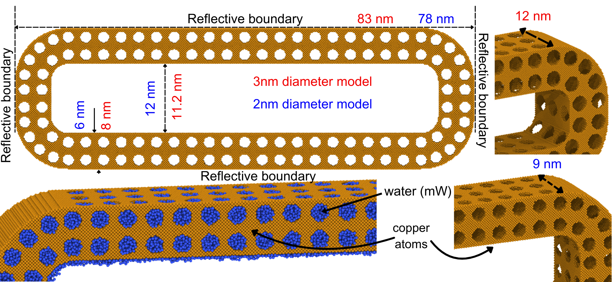
Figure 1: The top left panel shows boundary conditions and dimensions of the molecular systems used in this study, using the 2 nm model as a guide. The dimensions of the 2 nm model are labeled in blue, and those of the 3 nm model are shown in red. The top right shows a portion of the 3 nm model, and the bottom right shows the same for the 2 nm model.

To simulate the heat pipe at the nanoscale, two systems with varying levels of water inside are considered. The first system is a 3D porous heat pipe with 2 nm diameter holes drilled through it in all directions except at the corners, as shown in Figure 1. The length of the heat pipe is 78 nm, its thickness is 6 nm, and the gap inside is 12 nm. This gap is necessary for the vapor to travel to the cold side and condense.

The second system considered for the study is a pipe with 3 nm diameter holes, a length of 83 nm, a thickness of 8 nm, and a gap of 11.2 nm. The dimensions of both systems are labeled and shown in Figure 1. For clarity, only the image of the 2 nm system (henceforth called the 2 nm model) is shown, with labels in blue for the 2 nm model and red for the 3 nm model. The widths of the models are 9 nm and 12 nm, respectively.

The boundaries of the 2 nm model and the 3 nm model are reflective on the top, bottom, and sides, which contain the water molecules within the system boundaries. However, along the axis normal to the image, the boundary is periodic. The corners of the copper tube are covered with copper atoms with no holes to prevent water leakage into the empty space at the corners. The water molecules are shown in blue, and the copper atoms are shown in reddish-brown. The molecular details, especially the force field, will be discussed in the next section.

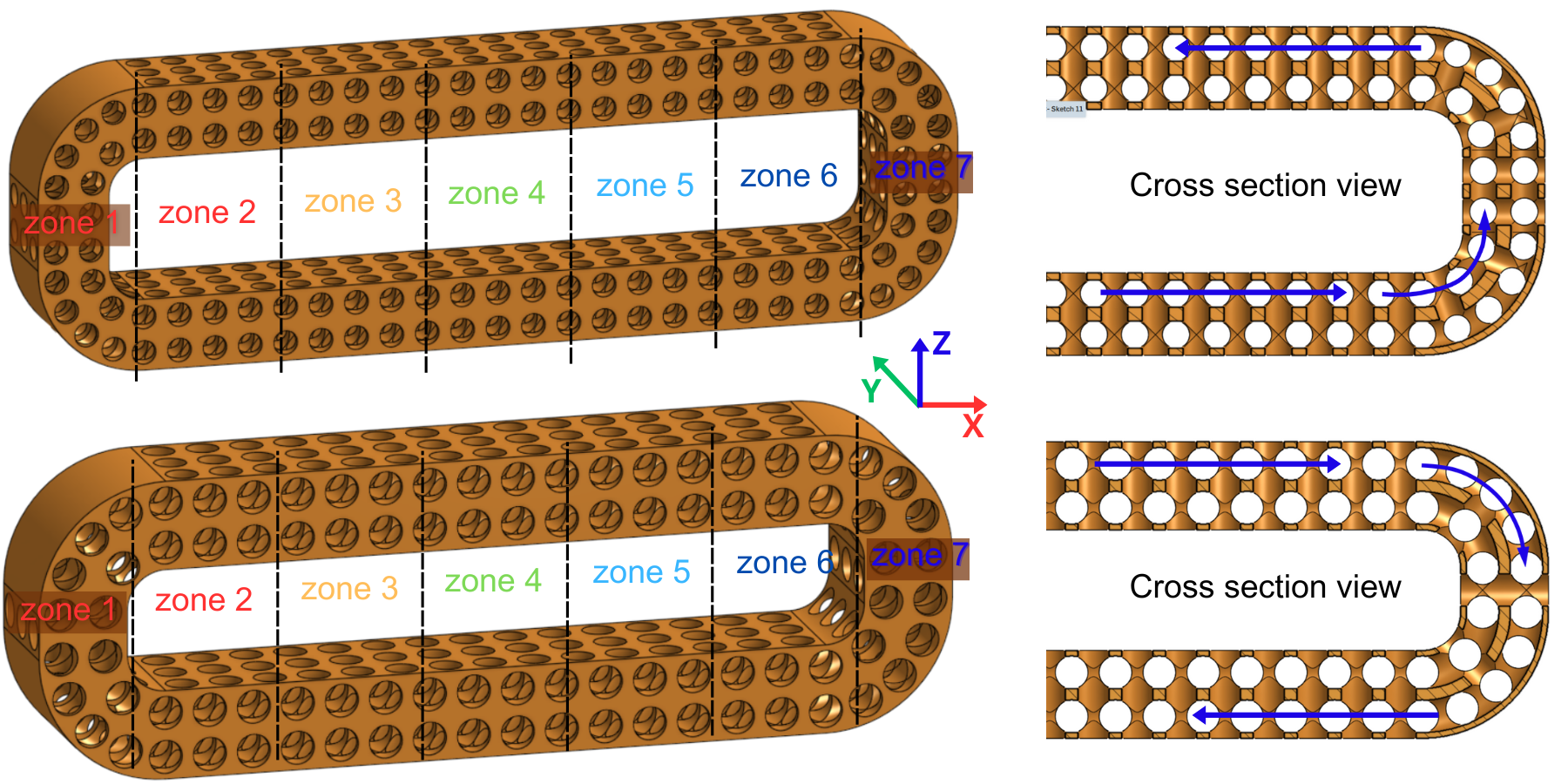
Figure 2: The 3D model images of both the 2 nm and 3 nm models are displayed in the top left and bottom left, respectively. Holes are drilled in the x, y, and z directions, except at the curved corners. At these curved corners, connectivity is maintained by linking the holes drilled along the x-axis and z-axis. The cross-sectional views shown in the top right and bottom right provide a clearer understanding of this connectivity. The arrows in these views illustrate the connectivity and are not intended to represent the fluid flow path.

Figure 2 illustrates the three-dimensional (3D) models of the 2 nm and 3 nm systems in an isometric perspective. These models represent the spatial arrangement of copper atoms within the system. To clarify the annular connectivity between the holes in both models, cross-sectional views are provided in the right panels of Figure 2. The axes of the geometry are depicted at the center for reference. The arrows in the cross-sectional views serve to demonstrate the connectivity within the system, rather than indicating the direction of water flow. The actual direction of water flow will be analyzed and detailed in the Results and Discussion section.

The molecular systems are virtually segmented into distinct zones to facilitate the application of temperature gradients to the water molecules. Figure 2 shows seven zones, with Zone 1 being the hottest and Zone 7 the coldest. Zone 1 and Zone 7 each span 10 nm from the respective ends, while the intermediate zones are equidistantly spaced. This zonal temperature application methodology is designed to prevent any artifacts or inaccuracies in the thermal boundary conditions.

In the scenario where the target temperature is 400K, Zone 1 is maintained at 400K, with a gradual decrease to 300K in Zone 7. Similarly, for the 350K case, Zone 1 is set at 350K, tapering down to 300K in Zone 7. Due to the dynamic nature of molecular systems, water molecules constantly migrate between these zones. Consequently, during the simulation, the temperature zones are updated at each step to reflect the precise number of water molecules in each zone. Although this process is computationally intensive, it is essential to ensure accurate and reliable simulation results.

To study the effect of the amount of water inside the system and its influence on circulation, we considered two levels of water. The system with excess water, referred to as “filled” throughout the paper, contains 248,178 water molecules for the 2 nm model and 443,158 water molecules for the 3 nm model. The models with the bare minimum amount of water necessary to wet the copper pipe (called “medfill”, resembling medium-fill) have 203,785 water molecules for the 2 nm model and 388,409 water molecules for the 3 nm model. The 2 nm model consists of 182,180 copper atoms, while the 3 nm model consists of 391,660 copper atoms.

III Molecular modeling details

In this study, the copper atoms are modeled using the Embedded Atom Model (EAM) [20, 21, 22, 23], with parameters sourced from the National Institute of Standards and Technology (NIST) database [24]. The copper atoms are represented within a Face-Centered Cubic (FCC) lattice structure, characterized by a lattice constant of 3.615 Å, ensuring a detailed and precise depiction of copper’s atomic arrangement. The porous nano structures are created by removing material by drilling holes of 2 nm diameter and 3nm diameter along the vertical and horizontal directions. Additionally, the holes are interconnected by drilling annular holes closely resembling the shape of the heat pipe. The EAM potential for copper, used in our study, is defined by Equation (1), with optimized parameters adopted from the widely used EAM potential for copper from literature [24].

$$E_{Cu-Cu}=F_{\alpha}\left(\sum_{j\neq i}{\rho_{\beta}\left(r_{ij}\right)}\right)+\frac{1}{2}\sum_{j\neq i}{\phi_{\alpha\beta}\left(r_{ij}\right)}$$ (1)

For the simulation of water molecules, instead of using the traditional computationally expensive models, a popular coarse grained model called mW model[17] is used. This model represents one water molecule by a coarse grained bead. The traditional models of water utilize long-range forces to replicate the hydrogen-bonded structure of water. The mW model diverges from this approach by introducing a short-range, angular-dependent term that promotes tetrahedrality. This model successfully reproduces the density, structure, and various phase transitions of water with high accuracy, at a significantly reduced computational cost compared to atomistic models. The mW model accurately reproduces water’s density maximum, melting temperature, and enthalpy of vaporization, among other properties. The results show that the structural and thermodynamic behavior of water can be effectively modeled by focusing on the tetrahedral connectivity of the molecules, rather than the nature of the interactions.

The equations governing this mW potential is based on the Stillinger-Weber model and is given in the below equations.

$$E_{mW-mW}=\sum_{i}\sum_{j>i}\phi_{2}(r_{ij})+\sum_{i}\sum_{j\neq i}\sum_{k>j}\phi_{3}(r_{ij},r_{ik},\theta_{ijk})$$ (2)

$$\phi_{2}(r_{ij})=A\epsilon\left[B\left(\frac{\sigma}{r_{ij}}\right)^{p}-\left(\frac{\sigma}{r_{ij}}\right)^{q}\right]\exp\left(\frac{\sigma}{r_{ij}-a\sigma}\right)$$ (3)

$$\phi_{3}(r_{ij},r_{ik},\theta_{ijk})=\lambda\epsilon\left(\cos\theta_{ijk}-\cos\theta_{0}\right)^{2}\exp\left(\frac{\sigma}{r_{ij}-a\sigma}\right)\exp\left(\frac{\sigma}{r_{ik}-a\sigma}\right)$$ (4)

The mW potential is sum of a two body interaction potential (3) and a three body interaction potential (4). The subscripts $i,j,k$ represents the three bodies (atoms/molecules) under consideration. The detailed explanation of this potential and relevance of each term is beyond the scope of this paper and readers are advised to refer the original work by Molinero [17].

The time step of integration is 10 fs, typical equilibration time is two million time steps and a production run is half a million time steps. The results are post processed using in house made C++ code [25] and MATLAB software [26]. The EAM potential of copper works well in the vicinity of 1 fs, which makes it unstable around 10 fs. Frequently, to circumvent this instability, we avoided the copper to copper interaction from time integration by freezing them and letting it interacting only with water molecules via Lennard-Jones potential. The motion of the copper atoms play less impact on coarse grained models and hence the freezing will not affect the dynamics of water much around it.

The water to copper interaction is modeled using the Lennard-Jones potential and uses the below equation (5).

$$E_{mW-Cu}=4\epsilon[(\sigma/r)^{12}-(\sigma/r)^{6}]$$ (5)

The interaction parameters of this potential is to simulate a hydrophilic nature of the water on copper, which based on the paper by Huang and et. al. [27].

IV Results and discussion

The molecular models described in the previous sections are utilized to simulate the heat pipe. For convenience, the cases are named according to the hole diameter, followed by the amount of water and the temperature at the left end of the pipe. For example, “2nm-medfill-400K-Density” refers to the density plot for a model with medium water fill, 2 nm diameter nanopores, and a left end temperature of 400K.

Initially, the heat pipe is modeled as a copper pipe, and water is introduced into it as a rectangular block. This water is absorbed by the nanopores, after which a new batch of water is introduced. The system is equilibrated for 500,000 time steps (5 ns), and this process is repeated until the pipe is completely wet. For the “filled” cases, the process continues until excess water accumulates in the inner region of the heat pipe.

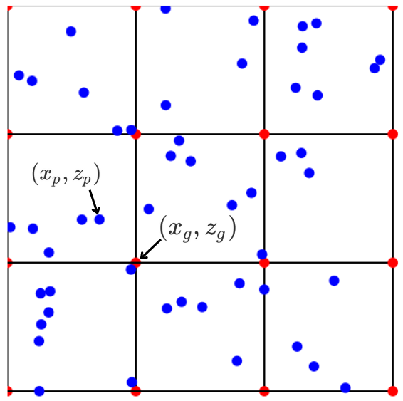
Figure 4: A sample representation of a segment of the hypothetical grid utilized for mapping molecular data to continuum-level properties is illustrated in the figure. In this representation, $(x_{p},z_{p})$ denotes the positions of particles (atoms), while $(x_{g},z_{g})$ indicates the coordinates of the grid points. This grid enables the conversion of discrete molecular information into a continuous field, helpful for the analysis of macroscopic properties.

Once equilibrated, the systems undergo production runs for at least 5 ns. During this period, a 2D grid-based approach is employed to map the statistical quantities to continuum-level properties. Figure 4 illustrates a sample representation of such a grid with grid points $(x_{g},z_{g})$ and particles at positions $(x_{p},z_{p})$. The properties of interest, computed at the particle positions, are interpolated onto the grid points using Nearest Grid Point (NGP) interpolation.

IV.1 Nearest Grid Point (NGP) Interpolation

In NGP interpolation, each particle’s property is assigned to the nearest grid point. This method is computationally efficient, though it may introduce aliasing errors. The grid value at a point $(x_{g},z_{g})$ is updated by accumulating the properties of particles nearest to this grid point.

Let $f(t,x_{p},z_{p})$ represent the property at particle position $(x_{p},z_{p})$ at time $t$. The grid value $f(t,x_{g},z_{g})$ at time $t$ is given by:

$$f(t,x_{g},z_{g})=\sum_{(x_{p},z_{p})\in\text{NGP}(x_{g},z_{g})}f(t,x_{p},z_{p})$$ (6)

where $\text{NGP}(x_{g},z_{g})$ denotes the set of particles nearest to the grid point $(x_{g},z_{g})$. A grid spacing of 1 nm is used for all our cases unless mentioned explicitly.

IV.2 Temporal Averaging

To reduce fluctuations and obtain smoother properties over time, temporal averaging is performed. Suppose we are averaging over $n$ time steps, with the property values at time steps $t_{1},t_{2},\ldots,t_{n}$. The temporally averaged property $\bar{f}(x_{g},z_{g})$ at the grid point $(x_{g},z_{g})$ is:

$$\bar{f}(x_{g},z_{g})=\frac{1}{n}\sum_{k=1}^{n}f(t_{k},x_{g},z_{g})$$ (7)

The following equations describe the interpolation of specific properties using NGP and temporal averaging.

IV.2.1 Velocity Components

For the velocity components $v_{x}$ and $v_{z}$:

$$v_{x}(t,x_{g},z_{g})=\sum_{(x_{p},z_{p})\in\text{NGP}(x_{g},z_{g})}v_{x}(t,x_{p},z_{p})$$ (8)

$$v_{z}(t,x_{g},z_{g})=\sum_{(x_{p},z_{p})\in\text{NGP}(x_{g},z_{g})}v_{z}(t,x_{p},z_{p})$$ (9)

Temporal averaging:

$$\bar{v}_{x}(x_{g},z_{g})=\frac{1}{n}\sum_{k=1}^{n}v_{x}(t_{k},x_{g},z_{g})$$ (10)

$$\bar{v}_{z}(x_{g},z_{g})=\frac{1}{n}\sum_{k=1}^{n}v_{z}(t_{k},x_{g},z_{g})$$ (11)

IV.2.2 Density

For the density $\rho$:

$$\rho(t,x_{g},z_{g})=\sum_{(x_{p},z_{p})\in\text{NGP}(x_{g},z_{g})}\rho(t,x_{p},z_{p})$$ (12)

Temporal averaging:

$$\bar{\rho}(x_{g},z_{g})=\frac{1}{n}\sum_{k=1}^{n}\rho(t_{k},x_{g},z_{g})$$ (13)

IV.2.3 Temperature

For the temperature $T$:

$$T(t,x_{g},z_{g})=\sum_{(x_{p},z_{p})\in\text{NGP}(x_{g},z_{g})}T(t,x_{p},z_{p})$$ (14)

Temporal averaging:

$$\bar{T}(x_{g},z_{g})=\frac{1}{n}\sum_{k=1}^{n}T(t_{k},x_{g},z_{g})$$ (15)

The properties of velocity, density, and temperature at grid points $(x_{g},z_{g})$ are estimated using the Nearest Grid Point (NGP) interpolation method. This involves assigning each particle’s property to the nearest grid point and performing temporal averaging over multiple time steps to smooth out fluctuations. The resulting plots, which illustrate these interpolations, are discussed in the following sections, providing a detailed explanation and analysis.

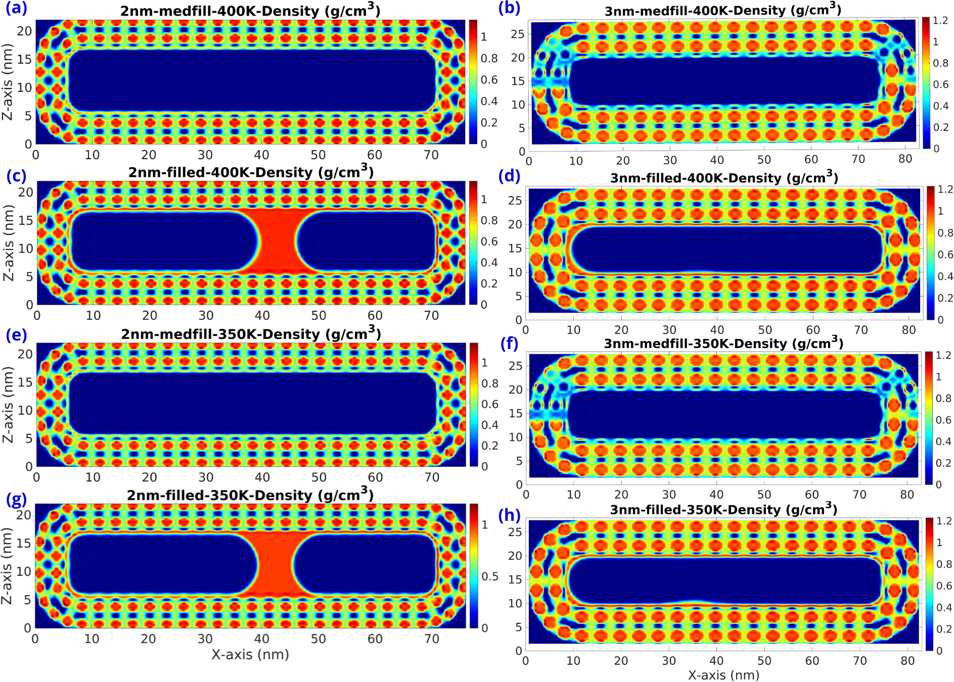
Figure 5: Density plots for 2nm model (1st column panels) and 3nm model (2nd column panels) are given for high temperature (400K) case in top four panels and low temperature (350K) case in bottom four panels. Medium filled water cases are given in panels a, b, e, and f and filled water cases are given in c, d, g and h respectively.

The mapped density plots for all cases are shown in Figure 5. The regions in red indicate high-density (liquid) water, while those in blue represent water vapor or vacuum. Areas with a mix of vapor and liquid follow the contour map on the right side of each panel. The “filled” 2 nm models exhibit a thick liquid connection suspended between the upper and lower surfaces of the heat pipe. Additionally, a thin layer of liquid water can be observed closer to the inner surface of the heat pipe in both cases, which is unsurprising due to the strong copper-to-water attraction.

The “medfill” cases of the 2 nm model at both 350K and 400K do not display any unexpected features. However, for the “medfill” cases of the 3 nm model at both 400K and 350K, there are less dense regions at either end of the heat pipe. This occurs because the water molecules did not completely fill these regions during the initial equilibration stage, rather than due to evaporation-induced voids. Interestingly, the “filled” 3 nm model cases show complete wetting within the heat pipe and a relatively thicker layer near the inner surface. This layer contributes to the movement of water from the hot region to the cold region and is the primary contributor to heat transfer. This analysis will be further discussed later in this section, along with the mass flow rate and heat transfer rate estimation.

IV.3 Vorticity

The vorticity $\omega$ in a 2D flow is defined as the curl of the velocity field. For a velocity field with components $v_{x}$ and $v_{z}$, the vorticity $\omega_{y}$ (since the system is periodic in y-axis, it’s a 2D flow, and the vorticity will be perpendicular to the $x$-$z$ plane) is given by [28, 29, 30, 31, 32]:

$$\omega_{y}=\frac{\partial v_{z}}{\partial x_{g}}-\frac{\partial v_{x}}{\partial z_{g}}$$ (16)

In a discrete grid like the one we described earlier, the partial derivatives can be approximated using finite difference methods. For example, using central differences, the derivatives can be approximated as:

$$\frac{\partial v_{z}}{\partial x_{g}}\approx\frac{v_{z}(x_{g}+\Delta x_{g},z_{g})-v_{z}(x_{g}-\Delta x_{g},z_{g})}{2\Delta x_{g}}$$ (17)

$$\frac{\partial v_{x}}{\partial z_{g}}\approx\frac{v_{x}(x_{g},z_{g}+\Delta z_{g})-v_{x}(x_{g},z_{g}-\Delta z_{g})}{2\Delta z_{g}}$$ (18)

Thus, the discrete form of the vorticity can be written as:

$$\omega_{y}(i,j)\approx\frac{v_{z}(i+1,j)-v_{z}(i-1,j)}{2\Delta x_{g}}$$ (19)

$$-\frac{v_{x}(i,j+1)-v_{x}(i,j-1)}{2\Delta z_{g}}$$

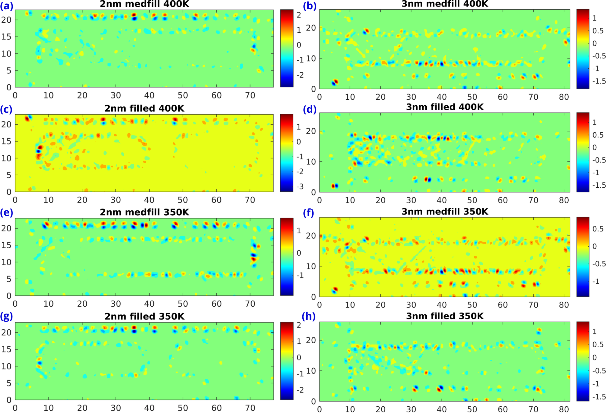
Figure 6: Vorticity plots for 2nm model (1st column panels) and 3nm model (2nd column panels) are given for high temperature (400K) case in top four panels and low temperature (350K) case in bottom four panels. Medium filled water cases are given in panels a, b, e, and f and filled water cases are given in c, d, g and h respectively.

Where $i$ and $j$ are the indices of the grid points in the $x_{g}$ and $z_{g}$ directions, respectively. The vorticity plots are shown in Figure 6. The regions in red indicate areas of positive vorticity, which signifies that the fluid in these regions is rotating counterclockwise. Conversely, the regions in blue indicate areas of negative vorticity, where the fluid is rotating clockwise. For the 2 nm ”medfill” cases (Figure 6. a, e, and the high temperature filled case Figure 6. g), the rotations are more localized inside the nanopores, particularly in the upper region. In the 2 nm filled high temperature case (Figure 6. c), rotational motion is observed not only within the nanopore cavities but also along the interior surface of the heat pipe.

For all cases of the 3 nm model, rotation is predominantly seen along the inner surface of the heat pipe. This observation suggests that the flow of water occurs primarily at the surface of the heat pipe rather than through the nanopore wicks. The vorticity results for the 2 nm model do not indicate significant flow within the pores. Instead, these results imply that fluid energy is absorbed and transferred, facilitating local rotation. This claim is further corroborated by the velocity profile findings discussed next.

In summary, the vorticity distribution reveals distinct rotational behavior dependent on nanopore size and temperature conditions. The 2 nm model exhibits localized vorticity within the nanopores, particularly under higher temperature conditions, while the 3 nm model shows a surface-dominated rotational flow.

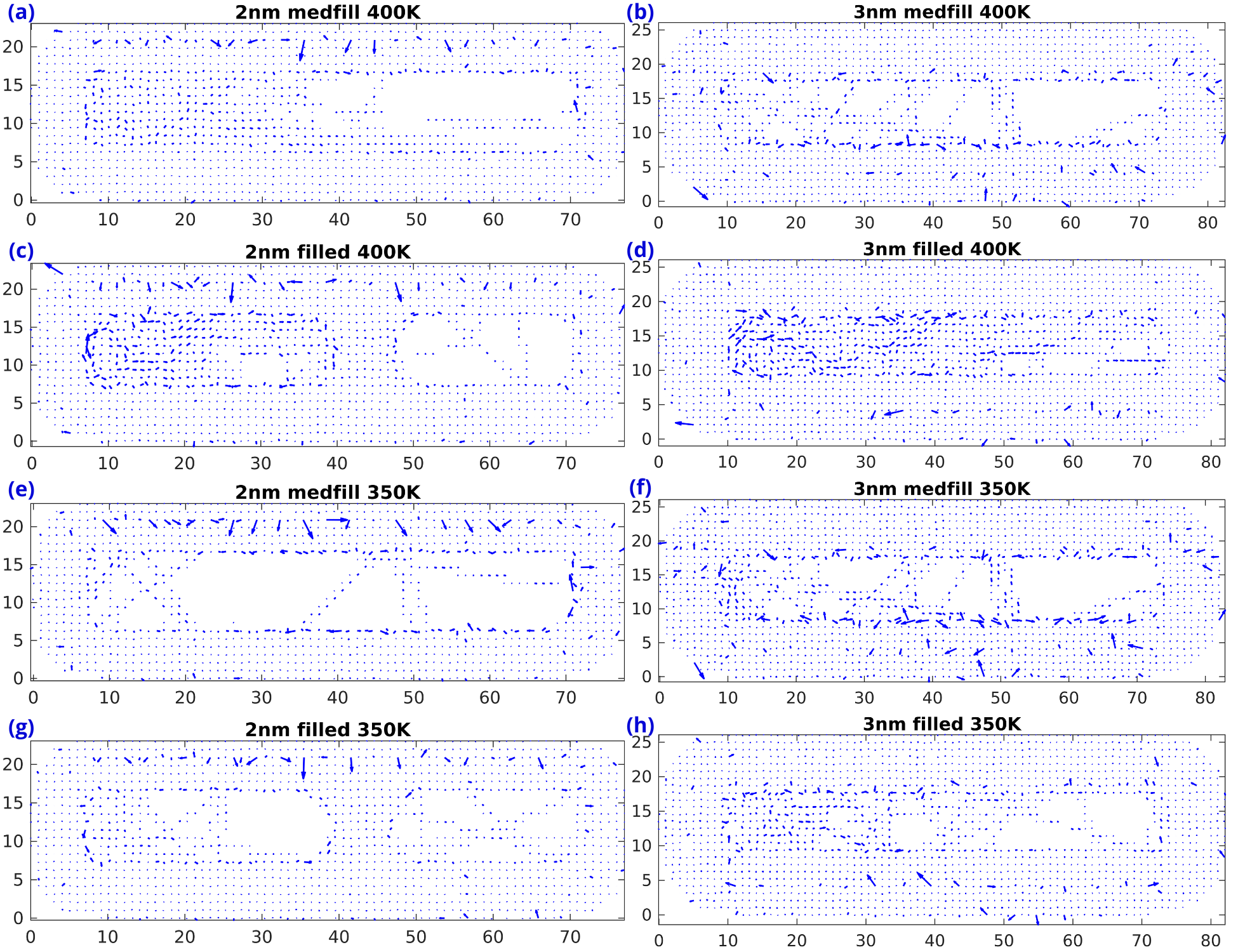
Figure 7: Velocity plots for 2nm model (1st column panels) and 3nm model (2nd column panels) are given for high temperature (400K) case in top four panels and low temperature (350K) case in bottom four panels. Medium filled water cases are given in panels a, b, e, and f and filled water cases are given in c, d, g and h respectively.

The velocity plots for all the cases studied in this project are shown in Figure 7. The 2 nm medfill cases (Figure 7 a and e) exhibit a continuous flow along the inner surface of the heat pipe, with stronger flows directed from the upper voids towards the lower regions. However, there is a lack of evidence suggesting a consistent pattern of heat transfer in these two cases.

For the 2 nm filled cases, the density plot indicates the formation of a thick water bridge between the upper and lower surfaces of the heat pipe. This bridge is sustained throughout the simulation and can be observed in the accompanying movie included in the supporting information. Figure 7 c) shows a strong recirculation of water along the inner surface in a clockwise direction. This recirculation is more pronounced at higher temperatures, particularly in the 400K case, and weaker in the 350K case (Figure 7 g).

The 3 nm cases reveal that no significant lateral flows occur within the nanopores. Instead, the flow is predominantly along the inner surface of the heat pipe. Notably, the left half of the lower surface experiences a leftward flow, while the lower right half experiences a rightward flow. The high-temperature case of the filled 3 nm model suggests increased evaporation at the hot section of the heat pipe. A similar effect is observed in the 350K case for the filled model, indicating enhanced evaporative cooling under elevated temperatures.

These observations provide insights into the fluid dynamics and heat transfer mechanisms within the nanoporous structures of the heat pipe, highlighting the influence of pore size and temperature on the overall performance. The sustained water bridge in the 2 nm cases suggests a stable liquid-vapor interface, which may contribute to localized heat transfer, while the 3 nm cases demonstrate surface-dominated flow patterns, emphasizing the importance of the inner surface in heat transport processes.

The velocity plot illustrates the arrow lengths corresponding to the magnitude, given by $|v|=\sqrt{v_{x}^{2}+v_{z}^{2}}$. This often poses challenges in visualizing the flow pattern within a region, particularly in areas with significantly lower velocities, such as the interior of the heat pipe wall compared to its surface. This visualization issue is evident in the plots shown in Figure 7, where the lower velocities inside the heat pipe wall make it difficult to discern the flow patterns.

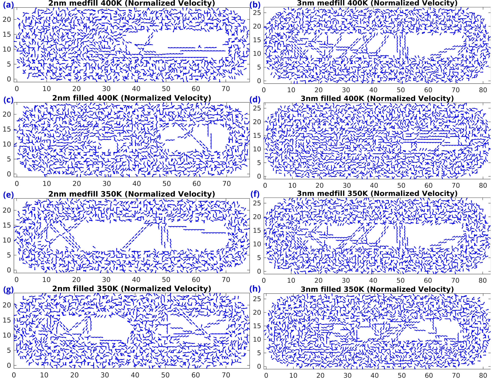
Figure 8: Normalized velocity plots for 2nm model (1st column panels) and 3nm model (2nd column panels) are given for high temperature (400K) case in top four panels and low temperature (350K) case in bottom four panels. Medium filled water cases are given in panels a, b, e, and f and filled water cases are given in c, d, g and h respectively.

To address this issue, we can use normalized velocity vectors, where a constant length is applied to all velocity values. This normalization helps in better visualizing the flow patterns by ensuring that even regions with low velocities are adequately represented. The normalized velocity plot, which employs a constant length for all velocity vectors, is shown in Figure 8.

This approach allows for a clearer representation of the flow dynamics throughout the heat pipe, providing a better understanding of the fluid behavior across different regions. The normalized plots help in identifying flow patterns that might be overlooked in the standard velocity plots, thus offering a more accurate depiction of the fluid motion within the heat pipe.

IV.4 Mass Flow Rate

The mass flow rate $\dot{m}$ $(kg/s)$ of the heat pipe is estimated by averaging the quantities over the entire 2D grid region, both temporally and spatially. This comprehensive approach ensures that the calculated mass flow rate accurately reflects the overall behavior of the heat pipe system under various conditions. The heat transfer rate $q$ $(W)$ can be estimated using the equation below:

$$q=\dot{m}c_{p}\Delta T$$ (20)

Where $c_{p}$ is the specific heat of water $(4187\ J/kg\cdot K)$ and $\Delta T$ is the temperature difference between the left and right ends of the heat pipe in Kelvin. This relationship underscores the direct dependence of the heat transfer rate on the mass flow rate, the specific heat capacity of the working fluid, and the temperature gradient across the heat pipe.

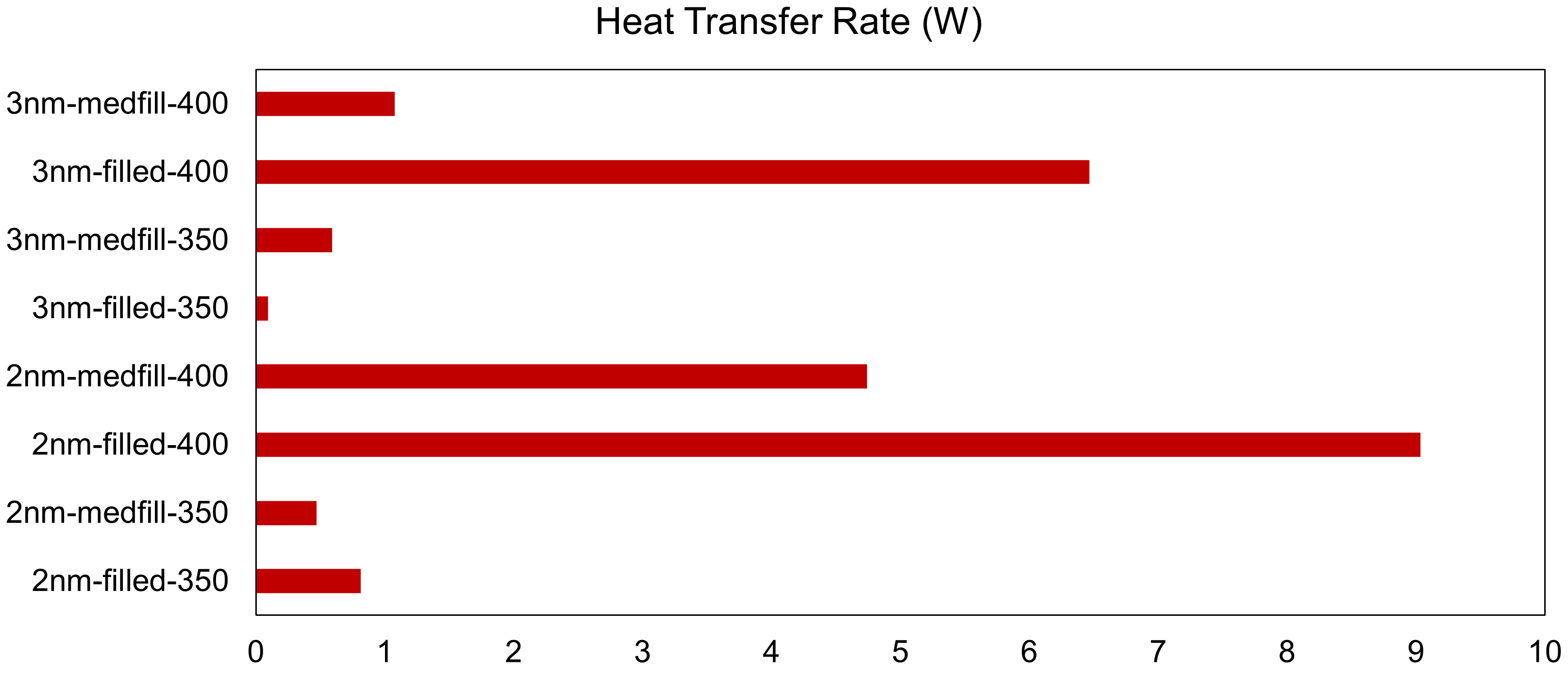
Figure 9: The heat transfer rate of the heat pipes under various conditions are shown in here. The x-axis represent heat transfer rate ($q$) and the y-axis represents various cases.

In our analysis, the averaged quantities of mass flow rate and temperature difference are plotted in Figure 9. The results indicate a clear trend where the cases at 400K exhibit a superior heat transfer performance compared to those at 350K. Specifically, the higher temperature gradient in the 400K cases enhances the driving force for heat transfer, thereby increasing the overall efficiency of the heat pipe.

Additionally, the data reveal that the ”filled” cases generally outperform the medium-filled cases in terms of heat transfer rate. This observation suggests that a higher fill ratio of the working fluid within the heat pipe improves the thermal performance, likely due to more effective phase change and fluid movement mechanisms.

Interestingly, the case with a 2nm fill ratio surpassed the 3nm model in terms of heat transfer rate performance. This counter intuitive result may be attributed to an optimal balance between capillary action and fluid flow resistance at the 2nm fill ratio, which maximizes the heat transfer efficiency.

For filled high-temperature cases, we observed heat transfer rates ranging from $6.5W$ to $9W$, which are comparable to the performance of heat pipes used in laptops and computers. Typically, laptop heat pipes can handle power levels around $25W$ to $52W$ depending on their design and application parameters [33, 34, 35, 36]. Our findings underscore the importance of optimizing both the operating temperature and fill ratio in the design and application of heat pipes for efficient thermal management. These analysis and comparisons of these variables provide insights into the thermal dynamics of heat pipes, guiding future improvements in their performance and application.

IV.5 Limitations and Scope for Improvements

IV.5.1 Selection of Water Molecules

Despite performing a comprehensive study on the system, we believe there are several factors that can be improved. The current study selected two levels of water with ”filled” indicating water content visibly excess inside the heat pipe and ”medfill” case with the bare minimum water for filling the nanopores. This selection is done through visual observation and can be improved systematically. The effect of water level on the heat transfer rate can be studied through a series of simulations of systems with varying levels of water, which will be computationally exhaustive. In fact, in the literature, there are no articles or technical documents explaining the accurate amount of water required based on a theoretical basis, which makes this problem a challenging one.

To address this challenge, future studies could adopt a systematic approach by incrementally varying the amount of water and performing detailed simulations for each level. This would provide a more accurate understanding of how the water content influences the heat transfer dynamics. Although this approach would require significant computational resources, it would offer valuable insights into optimizing the water level for enhanced thermal performance.

IV.5.2 Thermostatting Challenges and Alternatives

The proper way of performing a heat pipe simulation using molecular dynamics is to thermostat the copper atoms and then leave the water molecules for NVE (constant number of particles, volume, and energy) ensemble integration. Though in theory, this approach looks accurate, practically it creates an unstable system even within the lower ends of acceptable time steps of integration for coarse-grained molecular dynamics. An improvement in this context could be dividing the copper into tiny sections (probably 100+) and then thermostating the water within each section. This would require the remaining water within the inside of the heat pipe to be NVE integrated.

Although this approach is feasible, it can significantly slow down the computational process due to the need for frequent region updates. This is an area that could be explored further to develop more stable and efficient simulation techniques. Advanced thermostatting methods or hybrid approaches combining different ensembles could potentially mitigate these stability issues while maintaining computational efficiency.

IV.5.3 Ideal Length of Heat Pipe

There is no universally ideal length for a heat pipe; instead, it is often derived from the design and physical needs of the system under consideration. While the length can influence the mass flow rate and heat transfer rate, it is less likely to change the mode of heat transfer. Most dynamics settle down within the middle section of the heat pipe, suggesting that our model length is sufficient for this study.

However, future sensitivity studies could be performed to understand the effect of heat pipe length on various thermodynamic parameters. By varying the length and observing the resulting changes in performance, researchers can derive more precise guidelines for optimizing heat pipe dimensions in practical applications.

IV.5.4 Separation of Velocity Effects in Temperature and Pressure Estimation

One major observation while simulating the system with sub-critical nanopores is the bulk movement of water within the heat pipe. This bulk velocity can affect the calculation of temperature and pressure, as shown in Equations 21 and 22.

$$T=\frac{1}{3Nk_{B}}\sum_{i=1}^{N}m_{i}v_{i}^{2}$$ (21)

$$P=\frac{1}{V}\left(Nk_{B}T+\frac{1}{3}\sum_{i=1}^{N}\sum_{j>i}^{N}\mathbf{r}{ij}\cdot\mathbf{f}{ij}\right)$$ (22)

We attempted to correct for this by removing the center of mass velocity from the system and also by removing the bulk velocity for each grid point. However, this strategy did not significantly improve the results and its limitations can be observed in the temperature plots provided in the supplementary document.

Future work could explore more sophisticated techniques for separating the bulk velocity effects from the intrinsic thermal motions. For instance, advanced filtering methods or improved algorithms for velocity decomposition might provide better accuracy in estimating the true thermodynamic properties of the system.

V Conclusion

This study provides a comprehensive investigation into the thermal dynamics of heat pipes with sub-critical nanopores using coarse grain molecular dynamics simulations. By modeling water molecules and copper structures at the nanoscale, we have elucidated several key factors influencing the heat transfer efficiency in such systems.

The heat transfer rate is significantly higher in cases with a larger temperature difference, such as 400K compared to 350K. This is attributed to the enhanced driving force for thermal energy transport at larger temperature gradients. Additionally, filled cases, where the heat pipes contain a higher amount of water, demonstrate superior thermal performance compared to medium-filled cases due to more effective phase change processes and fluid dynamics within the heat pipe. Interestingly, the 2nm filled cases exhibit better heat transfer performance than the 3nm filled cases, suggesting an optimal balance between capillary action and fluid flow resistance at the 2nm fill ratio, which maximizes the heat transfer efficiency.

The vorticity and velocity analyses reveal distinct rotational behaviors and flow dynamics. The 2nm models show localized vorticity within the nanopores, especially at higher temperatures, while the 3nm models exhibit surface-dominated rotational flow, indicating that water flow primarily occurs along the inner surface of the heat pipe. The study indicates that surface-driven flows rather than wicking action dominate the heat transfer in heat pipes with sub-critical nano pores. This understanding can inform the design of nanostructures aimed at enhancing heat transfer via capillary flow.

These findings underscore the importance of optimizing both the operating temperature and fill ratio in the design and application of heat pipes for efficient thermal management. The results provide valuable insights into the thermal dynamics of heat pipes, guiding future improvements in their performance and application. Specifically, the optimal design would involve fine-tuning the nanopore size and fill ratio to balance capillary action and fluid flow resistance, thereby achieving maximum heat transfer efficiency. In conclusion, we believe that this study will advance our understanding of the thermal behavior of nanoporous heat pipes and offers practical guidelines for their design and optimization. The insights gained here will contribute to the development of more efficient thermal management solutions in various applications, particularly in electronics cooling and energy systems.

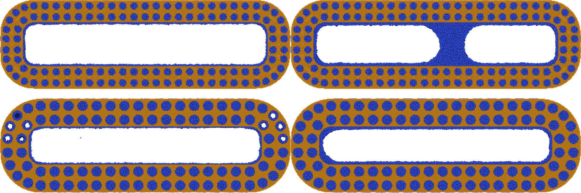
Figure 3: Equilibrated molecular models of the heat pipe with 2 nm holes filled with less water (top left), and with excess water (top right), and with 3 nm holes filled with less water (bottom left) and with excess water (bottom right).

References

- Garimella et al. [2016] S. V. Garimella, T. Persoons, J. A. Weibel, and V. Gektin, Electronics thermal management in information and communications technologies: Challenges and future directions, IEEE Transactions on Components, Packaging and Manufacturing Technology 7, 1191 (2016).
- Hu et al. [2020] R. Hu, Y. Liu, S. Shin, S. Huang, X. Ren, W. Shu, J. Cheng, G. Tao, W. Xu, R. Chen, et al., Emerging materials and strategies for personal thermal management, Advanced Energy Materials 10, 1903921 (2020).
- Khalaj and Halgamuge [2017] A. H. Khalaj and S. K. Halgamuge, A review on efficient thermal management of air-and liquid-cooled data centers: From chip to the cooling system, Applied Energy 205, 1165 (2017).
- Reed et al. [2022] D. Reed, D. Gannon, and J. Dongarra, Reinventing high performance computing: challenges and opportunities, arXiv preprint arXiv:2203.02544 (2022).
- Shalf [2020] J. Shalf, The future of computing beyond moore’s law, Philosophical Transactions of the Royal Society A 378, 20190061 (2020).
- Guo et al. [2020] H. Guo, X. Ji, and J. Xu, Enhancement of loop heat pipe heat transfer performance with superhydrophilic porous wick, International Journal of Thermal Sciences 156, 106466 (2020).
- Tang et al. [2023] H. Tang, Y. Xie, L. Xia, Y. Tang, and Y. Sun, Review on the fabrication of surface functional structures for enhancing heat transfer of heat pipes, Applied Thermal Engineering 226, 120337 (2023).
- Yi et al. [2023] F. Yi, Y. Gan, Z. Xin, Y. Li, and H. Chen, Experimental study on thermal performance of ultra-thin heat pipe with a novel composite wick structure, International Journal of Thermal Sciences 193, 108539 (2023).
- Alihosseini and Shafaee [2021] A. Alihosseini and M. Shafaee, Experimental study and numerical simulation of a lithium-ion battery thermal management system using a heat pipe, Journal of Energy Storage 39, 102616 (2021).
- Pawar and Sobhansarbandi [2020] V. R. Pawar and S. Sobhansarbandi, Cfd modeling of a thermal energy storage based heat pipe evacuated tube solar collector, Journal of Energy Storage 30, 101528 (2020).
- Behi et al. [2020] H. Behi, D. Karimi, M. Behi, J. Jaguemont, M. Ghanbarpour, M. Behnia, M. Berecibar, and J. Van Mierlo, Thermal management analysis using heat pipe in the high current discharging of lithium-ion battery in electric vehicles, Journal of Energy Storage 32, 101893 (2020).
- Daivis and Todd [2018] P. J. Daivis and B. D. Todd, Challenges in nanofluidics—beyond navier–stokes at the molecular scale, Processes 6, 144 (2018).
- Liu and Li [2011] C. Liu and Z. Li, On the validity of the navier-stokes equations for nanoscale liquid flows: The role of channel size, AIP Advances 1, 032108 (2011).
- Alami et al. [2023] A. H. Alami, M. Ramadan, M. Tawalbeh, S. Haridy, S. Al Abdulla, H. Aljaghoub, M. Ayoub, A. Alashkar, M. A. Abdelkareem, and A. G. Olabi, A critical insight on nanofluids for heat transfer enhancement, Scientific Reports 13, 15303 (2023).
- McCabe and Hadley [2012] C. McCabe and K. R. Hadley, Improved coarse-grained model for molecular-dynamics simulations of water nucleation, The Journal of Chemical Physics 136, 054510 (2012).
- Ouyang and Bettens [2015] J. F. Ouyang and R. P. Bettens, Unraveling thermodynamic anomalies of water: A molecular simulation approach to probe the two-state theory with atomistic and coarse-grained water models, The Journal of Chemical Physics 142, 054505 (2015).
- Molinero and Moore [2009] V. Molinero and E. B. Moore, Water modeled as an intermediate element between carbon and silicon, The Journal of Physical Chemistry B 113, 4008 (2009).
- Yesudasan [2022] S. Yesudasan, The critical diameter for continuous evaporation is between 3 and 4 nm for hydrophilic nanopores, Langmuir 38, 6550 (2022).
- Yesudasan [2020] S. Yesudasan, Extended martini water model for heat transfer studies, Molecular Physics 118, e1692151 (2020).
- Zarringhalam et al. [2019] M. Zarringhalam, H. Ahmadi-Danesh-Ashtiani, D. Toghraie, and R. Fazaeli, The effects of suspending copper nanoparticles into argon base fluid inside a microchannel under boiling flow condition by using of molecular dynamic simulation, Journal of Molecular Liquids 293, 111474 (2019).
- Lysogorskiy et al. [2021] Y. Lysogorskiy, C. v. d. Oord, A. Bochkarev, S. Menon, M. Rinaldi, T. Hammerschmidt, M. Mrovec, A. Thompson, G. Csányi, C. Ortner, et al., Performant implementation of the atomic cluster expansion (pace) and application to copper and silicon, npj Computational Materials 7, 97 (2021).
- Fairushin et al. [2020] I. Fairushin, A. Saifutdinov, and A. Sofronitskiy, Numerical and experimental studies of the synthesis of copper nanoparticles in a high-pressure discharge, High Energy Chemistry 54, 150 (2020).
- Cometto et al. [2021] C. Cometto, A. Ugolotti, E. Grazietti, A. Moretto, G. Bottaro, L. Armelao, C. Di Valentin, L. Calvillo, and G. Granozzi, Copper single-atoms embedded in 2d graphitic carbon nitride for the co2 reduction, npj 2D Materials and Applications 5, 63 (2021).
- Zuo et al. [2020] Y. Zuo, C. Chen, X. Li, Z. Deng, Y. Chen, J. Behler, G. Csányi, A. V. Shapeev, A. P. Thompson, M. A. Wood, et al., Performance and cost assessment of machine learning interatomic potentials, The Journal of Physical Chemistry A 124, 731 (2020).
- ISO/IEC [2003] ISO/IEC, The C++ Standard: Incorporating Technical Corrigendum No. 1, International Organization for Standardization, Geneva, Switzerland (2003), iSO/IEC 14882:2003(E).
- The MathWorks Inc. [2022] The MathWorks Inc., MATLAB and Simulink Release 2022b (2022), natick, Massachusetts, United States.
- Huang et al. [2023] X. Huang, L. Zhou, and X. Du, Critical contact angle for triggering dynamic leidenfrost phenomenon at different surface wettability: A molecular dynamics study, Journal of Molecular Liquids 382, 121982 (2023).
- Batchelor [1988] G. Batchelor, An Introduction to Fluid Dynamics (Cambridge University Press, 1988).
- Ferziger and Perić [2002] J. Ferziger and M. Perić, Computational Methods for Fluid Dynamics (Springer, 2002).
- Hirsch [1988] C. Hirsch, Numerical Computation of Internal and External Flows (Wiley, 1988).
- SpringerLink [2022] SpringerLink, Fluid Dynamics: Solving the 2D Navier–Stokes Equations (Springer, 2022).
- Oceanography [2022] P. A. Oceanography, The Curl, and Vorticity – Physics Across Oceanography: Fluid Mechanics and Waves (University of Washington Press, 2022).
- Celsia Inc. [2022] Celsia Inc., Heat pipe design guide (2022).
- Electronics Cooling [2022] Electronics Cooling, Design considerations when using heat pipes (2022).
- Byon [2016] C. Byon, Heat pipe and phase change heat transfer technologies for electronics cooling, in Electronics Cooling, edited by S. M. S. Murshed (IntechOpen, Rijeka, 2016) Chap. 3.
- Advanced Cooling Technologies Inc. [2022] Advanced Cooling Technologies Inc., Heat pipes 101 (2022).