Eliciting prior information from clinical trials via calibrated Bayes factor

Abstract

In the Bayesian framework power prior distributions are increasingly adopted in clinical trials and similar studies to incorporate external and past information, typically to inform the parameter associated to a treatment effect. Their use is particularly effective in scenarios with small sample sizes and where robust prior information is actually available. A crucial component of this methodology is represented by its weight parameter, which controls the volume of historical information incorporated into the current analysis. This parameter can be considered as either fixed or random. Although various strategies exist for its determination, eliciting the prior distribution of the weight parameter according to a full Bayesian approach remains a challenge. In general, this parameter should be carefully selected to accurately reflect the available prior information without dominating the posterior inferential conclusions. To this aim, we propose a novel method for eliciting the prior distribution of the weight parameter through a simulation-based calibrated Bayes factor procedure. This approach allows for the prior distribution to be updated based on the strength of evidence provided by the data: The goal is to facilitate the integration of historical data when it aligns with current information and to limit it when discrepancies arise in terms, for instance, of prior-data conflicts. The performance of the proposed method is tested through simulation studies and applied to real data from clinical trials.
Keywords: Dynamic borrowing, Historical data, Power prior, Prior elicitation, Strength of evidence

1 Introduction

In recent years, biostatistical applications are commonly characterized by insufficient sample sizes, which are crucial for accurate parameter estimation. Meanwhile, in the clinical framework a large amount of historical or related data are often available. This has led to a growing interest in using historical data to enhance the design and analysis of new studies, particularly in clinical trials where recruiting patients can be ethically challenging. Notably, the sequential nature of information updating has made Bayesian approaches with informative priors particularly popular in this context (Chen and Ibrahim, , 2000; Hobbs et al., , 2012; Ollier et al., , 2020; Schmidli et al., , 2014; Neuenschwander and Schmidli, , 2020, among others). These methods facilitate the incorporation of historical data into the analysis by eliciting informative priors on the model parameters, thereby improving the robustness and efficiency of statistical inference. However, the elicitation of informative priors is widely recognized as a complex process due to the challenges in quantifying and synthesizing prior information into suitable prior distributions. For an in-depth and comprehensive analysis of the topic see Spiegelhalter et al., (1994, 2004). Consequently, there is a pressing need to develop more efficient methods for synthesizing and quantifying prior information (Ibrahim et al., , 2015). Specifically, there is a growing concern regarding the adaptive incorporation of historical data, especially in the presence of data heterogeneity and rapid changes in the initial trial conditions (Ollier et al., , 2020).

In this framework, the power prior (Chen and Ibrahim, , 2000) is a popular method that allows historical data to influence the prior distribution in a flexible and controlled way. Ibrahim et al., (2003) provided a formal justification for power priors, demonstrating their effectiveness as a valuable class of informative priors. This effectiveness stems from their ability to minimize a convex sum of Kullback-Leibler (KL) divergences between two distinct posterior densities, in which one does not include any historical data whereas the other fully integrates this information into the current analysis. Additionally, De Santis, (2006) proposed further operational justifications, linking them to the so-called geometric priors. Notably, power priors have been employed across a broad spectrum of models including generalized linear models (GLMs), generalized linear mixed models (GLMMs), and survival models (Chen et al., , 2000; Chen and Ibrahim, , 2006; Ibrahim et al., , 2015). At its core, the idea is to raise the likelihood of the historical data to a weight parameter $\delta$, usually defined between zero and one. This scalar parameter plays a crucial role in the power prior methodology as it determines the degree to which historical data influences the prior distribution. Specifically, when $\delta$ is set to zero, the power prior completely discounts historical information; conversely, setting $\delta$ to one fully integrates historical information into the prior.

As is intuitive, the role played by the weight parameter $\delta$ on the final inferential conclusions is not negligible. Thus, several strategies have been developed to specify the weight parameter $\delta$, treating it either as a fixed or a random quantity. If fixed in advance, the weight parameter $\delta$ can be set based on prior knowledge or through sensitivity analysis, considering specific criteria for borrowing information based on the prior-data conflict (Evans and Moshonov, , 2006; Egidi et al., , 2022). If treated as random, an initial prior distribution – typically a Beta distribution – is assigned to $\delta$, and the use of the joint normalized power prior (Duan et al., , 2006; Neuenschwander et al., , 2009) is recommended. Notably, Nikolakopoulos et al., (2018) introduced a method to estimate this parameter using predictive distributions, aiming at controlling type I error by calibrating to the degree of similarity between the current and historical data. Furthermore, Liu, (2018) recommended setting $\delta$ through a dynamic p-value, assessing the compatibility of current and historical data based on the test‐then‐pool methodology. Gravestock and Held, (2017, 2019) proposed an empirical Bayes-type approach for estimating the weight parameter by maximizing the marginal likelihood. Bennett et al., (2021) suggested two novel approaches for binary data, focusing on equivalence probability and tail area probabilities. Mariani et al., (2024) explored the use of the Hellinger distance to compare the posterior distributions of the control parameter from current and historical data, respectively. These techniques provide valuable insights on determining a specific fixed value for $\delta$. However, in a fully Bayesian context, only Shen et al., (2023) has developed methods for specifying the shape parameters of a Beta initial prior for $\delta$, using two minimization criteria: Kullback-Leibler (KL) divergence and mean squared error (MSE). Therefore, in a fully Bayesian framework, eliciting the initial distribution of the weight parameter controlling the amount of historical information remains a challenging and underexplored area.

The aim of this paper is to propose a novel Bayesian algorithmic approach for eliciting the initial prior distribution for $\delta$ in a somehow optimal way. This involves the use of a simulation-based calibrated Bayes factor, employing hypothetical replications generated from the posterior predictive distribution, to compare competing prior distributions for $\delta$. Following the approach in Shen et al., (2023), a well-balanced prior should promote the integration of historical data when there is agreement with the current information, and limiting this integration when discrepancies between the two datasets arise.

The paper is organized as follows. Section 2 provides a review of the power prior methodology, discussing the use of the weight parameter as both a fixed and a random quantity. Furthermore, Section 3 illustrates the proposed calibrated Bayes factor to elicit a well-balanced initial prior distribution for $\delta$. Sections 4 and 5 explore the proposed methodology through simulation studies and real data analysis from two clinical trials, E2696 and E1694, that investigated the effectiveness of interferon in melanoma treatment (Kirkwood et al., 2001a, ; Kirkwood et al., 2001b, ). Finally, Section 6 provides concluding remarks about the discussed method, highlighting its strengths and limitations, and offers insights into future developments.

2 Power priors

Power priors have become increasingly popular for the development of informative priors, especially in clinical trials where past information is often available. These priors effectively integrate knowledge from historical data into the specification of informative priors. Let consider $\boldsymbol{\theta}$ as the vector parameter of interest in the model, and let $y_{0}$ represent the historical data with its corresponding likelihood function denoted by $L(\boldsymbol{\theta}\mid y_{0})$. The basic formulation of the power prior (Chen and Ibrahim, , 2000) is given by

$$\pi(\boldsymbol{\theta}\mid y_{0},\delta)\propto L(\boldsymbol{\theta}\mid y_{0})^{\delta}\pi_{0}(\boldsymbol{\theta}),$$ (1)

where $\delta\in[0,1]$ is the scalar weight parameter, and $\pi_{0}(\boldsymbol{\theta})$ is the initial – often non-informative – prior for $\boldsymbol{\theta}$. This model can be seen as a generalization of the classical Bayesian updating of $\pi_{0}(\boldsymbol{\theta})$. Additionally, as noted by Ibrahim et al., (2015), the parameter $\delta$ plays a crucial role in determining the shape of the prior distribution for $\boldsymbol{\theta}$. Furthermore, updating the power prior in (1) with the current data likelihood $L(\boldsymbol{\theta}\mid y)$ yields the following posterior distribution of $\boldsymbol{\theta}$

$$\pi(\boldsymbol{\theta}\mid y,y_{0},\delta)\propto L(\boldsymbol{\theta}\mid y)L(\boldsymbol{\theta}\mid y_{0})^{\delta}\pi_{0}(\boldsymbol{\theta}).$$

The formulation in (1) is conditional on the weight parameter and requires a predetermined and known value for $\delta$. Therefore, to ensure an appropriate level of historical information borrowing while managing prior-data conflict, sensitivity analysis is recommended. In addition to the dynamic methods outlined in the introduction, Ibrahim et al., (2015) also proposed several other statistical methods, including the Penalized Likelihood-type Criterion (PLC), Marginal Likelihood Criterion (MLC), Deviance Information Criterion (DIC), and the Logarithm of the Pseudo-Marginal Likelihood (LPML) Criterion.

2.1 Hierarchical power priors

A natural extension of the power prior in (1) can be achieved by accounting for uncertainty about the weight parameter $\delta$. This involves adopting a hierarchical power prior where $\delta$ is treated as a random variable. To achieve this, a Beta prior distribution is assigned to $\delta$, leading to the so-called joint unnormalized power prior (Chen and Ibrahim, , 2000) for both $\boldsymbol{\theta}$ and $\delta$

$$\pi(\boldsymbol{\theta},\delta\mid y_{0}) =\pi(\boldsymbol{\theta}\mid y_{0},\delta)\pi_{0}(\delta)$$ (2)

$$\propto L(\boldsymbol{\theta}\mid y_{0})^{\delta}\pi_{0}(\boldsymbol{\theta})\pi_{0}(\delta),$$

where $\pi_{0}(\boldsymbol{\theta})$ and $\pi_{0}(\delta)$ represent the initial priors for $\boldsymbol{\theta}$ and $\delta$, respectively.

However, as noted by Duan et al., (2006) and Neuenschwander et al., (2009), the formulation in (2) lacks of a normalizing constant, leading to potential inconsistencies in the joint posterior distributions for $(\boldsymbol{\theta},\delta)$ derived from different forms of likelihood functions, such as those based on raw data versus those based on the distribution of sufficient statistics (Ye et al., , 2022). Consequently, Duan et al., (2006) proposed a normalized power prior which involves first setting a conditional prior on $\boldsymbol{\theta}$ given $\delta$, followed by an initial prior distribution for $\delta$. The resulting joint normalized power prior for $(\boldsymbol{\theta},\delta)$ is

$$\pi\left(\boldsymbol{\theta},\delta\mid y_{0}\right) =\pi(\boldsymbol{\theta}\mid y_{0},\delta)\pi_{0}(\delta)$$ (3)

$$=\frac{L\left(\boldsymbol{\theta}\mid y_{0}\right)^{\delta}\pi_{0}(\boldsymbol{\theta})}{C(\delta)}\pi_{0}(\delta),$$

where the normalizing constant $C(\delta)$ is

$$C(\delta)=\int_{\Theta}L(\boldsymbol{\theta}\mid y_{0})^{\delta}\pi_{0}(\boldsymbol{\theta})\mathrm{d}\boldsymbol{\theta}.$$ (4)

In light of the current data the joint posterior distribution is

$$\pi\left(\boldsymbol{\theta},\delta\mid y,y_{0}\right) =\frac{L(\boldsymbol{\theta}\mid y)\pi\left(\boldsymbol{\theta},\delta\mid y_{0}\right)}{\int_{0}^{1}\int_{\Theta}L(\boldsymbol{\theta}\mid y)\pi\left(\boldsymbol{\theta},\delta\mid y_{0}\right)\mathrm{d}\boldsymbol{\theta}\mathrm{d}\delta}$$ (5)

$$\propto L(\boldsymbol{\theta}\mid y)\frac{L\left(\boldsymbol{\theta}\mid y_{0}\right)^{\delta}\pi_{0}(\boldsymbol{\theta})}{C(\delta)}\pi_{0}(\delta).$$

The marginal posterior distribution of $\delta$ is

$$\pi\left(\delta\mid y,y_{0}\right)\propto\frac{\pi_{0}(\delta)}{C(\delta)}\int_{\Theta}L(\boldsymbol{\theta}\mid y)L\left(\boldsymbol{\theta}\mid y_{0}\right)^{\delta}\pi_{0}(\boldsymbol{\theta})\mathrm{d}\boldsymbol{\theta}.$$

Integrating $\delta$ out in (5), the marginal posterior of $\boldsymbol{\theta}$ can be written as

$$\pi\left(\boldsymbol{\theta}\mid y,y_{0}\right)\propto\pi_{0}(\boldsymbol{\theta})L(\boldsymbol{\theta}\mid y)\int_{0}^{1}\frac{L(\boldsymbol{\theta}\mid y_{0})^{\delta}\pi_{0}(\delta)}{C(\delta)}\mathrm{d}\delta.$$

The joint power prior framework offers the advantage of incorporating uncertainty regarding the weight parameter $\delta$ into the power prior formulation. This approach allows the data to determine the appropriate weight for historical information based on its compatibility with current observations. Furthermore, explicitly accounting for this uncertainty increases the flexibility in modeling the agreement between historical and current data.

In addition, a crucial theoretical advantage of the joint normalized power prior formulation with respect to the formulation in (2) is its adherence to the likelihood principle. This ensures that the posterior distributions in (5) accurately reflect the compatibility between current and historical data. Furthermore, this approach has further theoretically justification, as the power prior formulation in (3) is shown to minimize the weighted KL divergence (Ye et al., , 2022).

From a computational perspective, the additional effort required for the normalized power prior compared to the unnormalized power prior involves computing the normalizing constant in (4). For certain models, this integral can be solved analytically, resulting in a closed-form expression for the joint posterior as specified in (5). However, for more complex models, the normalizing constant $C(\delta)$ must be determined numerically. Consequently, the posterior distribution in (5) falls into the category of the doubly intractable distributions (Carvalho and Ibrahim, , 2021), and numerical methods such as Markov Chain Monte Carlo (MCMC) (Robert and Casella, , 2004) are required.

3 The calibrated Bayes factor

Eliciting a well-balanced initial prior distribution for $\delta$ has proven to be challenging. Intuitively, this prior should encourage borrowing when the data are compatible and limit borrowing when they are in conflict. In this section, we propose a calibrated Bayes factor, hereafter CBF, that is a simulation-based algorithmic technique designed to effectively discriminate between some competing initial Beta prior distributions for $\delta$. The proposed CBF aims to provide more robust decisions about which initial Beta prior for $\delta$ may be used. Specifically, this involves analyzing the behaviour of the Bayes factor (Jeffreys, , 1961; Kass, , 1993; Kass and Raftery, , 1995), henceforth BF, using different hypothetical replications generated from the posterior predictive distributions, while assessing how surprising the observed value of the Bayes factor is.

3.1 The Bayes factor

The BF provides a general Bayesian method to assess the relative evidence in support of competing hypotheses based on their compatibility with the observed data. Furthermore, the BF represents the ratio between the posterior and the prior odds when comparing two distinct point hypotheses. Specifically, let consider two competing hypotheses about the initial prior distribution on the weight parameter

$$\delta\mid\mathcal{H}_{0}\sim\mathrm{Beta}(\eta_{0},\nu_{0})\;\text{ vs. }\;\delta\mid\mathcal{H}_{1}\sim\mathrm{Beta}(\eta_{1},\nu_{1}),$$

where $\eta_{i}$ and $\nu_{i}$ represent the strictly positive Beta shape parameters under the hypothesis $\mathcal{H}_{i}$, for $i=\left\{0,1\right\}$. The corresponding Bayes factor can be expressed as the ratio of the two marginal likelihoods

$$\mathrm{BF}_{0,1}(y) =\dfrac{m(y\mid\mathcal{H}_{1})}{m(y\mid\mathcal{H}_{0})},$$ (6)

where the marginal likelihood is

$$m(y\mid\mathcal{H}_{i})=\int_{0}^{1}\dfrac{\int_{\Theta}L\left(\boldsymbol{\theta}\mid y\right)L\left(\boldsymbol{\theta}\mid y_{0}\right)^{\delta}\pi_{0}(\boldsymbol{\theta})\pi_{0}(\delta\mid\mathcal{H}_{i})\mathrm{d}\boldsymbol{\theta}}{\int_{\Theta}L\left(\boldsymbol{\theta}\mid y_{0}\right)^{\delta}\pi_{0}(\boldsymbol{\theta})\mathrm{d}\boldsymbol{\theta}}\mathrm{d}\delta,$$

with $\pi_{0}(\delta\mid\mathcal{H}_{i})$ representing the initial Beta prior distribution for $\delta$ under the hypothesis $\mathcal{H}_{i}$, for $i=\left\{0,1\right\}$. Assuming equal prior probabilities for both the models, a BF exceeding one suggests stronger evidence in favor of $\mathcal{H}_{1}$. Conversely, a BF below one denotes a stronger evidence for $\mathcal{H}_{0}$. A BF close to one indicates no clear preference for either hypothesis, reflecting a similar degree of empirical evidence for both $\mathcal{H}_{0}$ and $\mathcal{H}_{1}$. Several approaches have been developed to summarize and classify the strength of evidence according to the observed BF. Firstly, Jeffreys, (1961) introduced a categorization, as illustrated in Table 1. Subsequently, Kass and Raftery, (1995) streamlined this scale by omitting one category and redefining the thresholds. Lastly, Lee and Wagenmakers, (2014, Table 7.1, p.105) further refined Jeffreys’ scale with additional modifications.

For most complex models the BF computation is challenging since the marginal likelihood is not analytically tractable. Therefore, numerical approximation methods become essential. A widely used algorithm is the so-called bridge sampling (Meng and Wong, , 1996). This method employs a Monte Carlo technique, generating samples from an auxiliary distribution that bridges the model’s prior and posterior distribution. The generated samples are then used to calculate bridge sampling weights, which correct the bias introduced by the auxiliary distribution, providing an unbiased estimate of the marginal likelihood.

Another noteworthy method is the Savage–Dickey algorithm (Dickey and Lientz, , 1970). This method approximates the BF by calculating the ratio of the posterior and prior densities at a model parameter value of zero. However, its use is limited to nested models and may be unstable if the posterior density significantly deviates from zero.

Table 1: Scale of evidence for the BF proposed by Jeffreys, (1961).

$\mathrm{BF}_{0,1}$	$\log_{10}(\mathrm{BF}_{0,1})$	Evidence Category
$1$ - $3.16$	$0$ - $0.5$	Barely worth mentioning
$3.16$ - $10$	$0.5$ - $1$	Substantial evidence for $\mathcal{H}_{1}$
$10$ - $31.62$	$1$ - $1.5$	Strong evidence for $\mathcal{H}_{1}$
$31.62$ - $100$	$1.5$ - $2$	Very strong evidence for $\mathcal{H}_{1}$
$>100$	$>2$	Decisive evidence for $\mathcal{H}_{1}$

3.2 Simulation-based calibration

The BF has an inherent dependence on the observed data when used for decision-making. Consequently, decisions based solely on current observations may lead to potentially misleading conclusions due to the possible fluctuations and noise present in the data. Furthermore, Schad et al., (2023) emphasized two crucial issues regarding BF computations: the instability of BF estimates in complex statistical models and the potential bias within these estimates. Therefore, to effectively and responsibly employ the BF, it is crucial to adjust and calibrate it, ensuring that the conclusions drawn are more robust and reliable.

The concept of simulation-based calibration, hereafter SBC, was originally developed to validate the computational correctness of applied Bayesian inference methods (Geweke, , 2004; Cook et al., , 2006; Talts et al., , 2018; Gelman et al., , 2020; Schad et al., , 2021; Modrák et al., , 2023, among others). In addition, Schad et al., (2023) proposed a structured approach based on SBC to verify the accuracy of BF calculations. Their calibration method involves simulating multiple artificial datasets to assess whether a BF estimated in a given analysis is accurate or biased. This type of calibration approach is intuitive and logical, as it mirrors the classical approach of hypothesis testing, where the decision-making criterion is determined by the sampling distribution under the hypothesis of repeated sampling.

The SBC-inspired method explored in this paper is motivated by the insights of Garcia-Donato and Chen, (2005), who posited that the BF should be considered as a random variable before observing the sample. This perspective emphasizes the necessity of calibrating the BF to accurately account for the inherent randomness in the data. However, the analytic form of the BF distribution is frequently not available. In such cases, a simulation-intensive approach becomes a valuable tool for approximating this distribution (Vlachos and Gelfand, , 2003). This involves generating replicated datasets from some type of predictive distribution or other data-generating processes, estimating the marginal likelihoods with these synthetic datasets, and then computing the BFs. By iterating this process multiple times, an approximation of the BF distribution is obtained. Subsequently, once the data have been collected, the observed BF can be used as a measure of agreement between the observed data and the underline statistical model.

Both Garcia-Donato and Chen, (2005) and Schad et al., (2023) suggested a calibration method based on the prior predictive distribution. However, this approach is not suitable in our context due to the inherent bias in the replicated data from the prior predictive distribution towards the historical data $y_{0}$, as highlighted by the structure of Equation (3). This can potentially yield replicated samples that are much more in agreement with the historical data than the historical data are with the current data. Consequently, we explored the use of hypothetical replications generated from the posterior predictive distribution to approximate the distribution of the BF; where the predictive distribution is given by

$$p\left(y^{\text{rep }}\mid y\right)=\int_{\Theta}L\left(y^{\text{rep }}\mid\boldsymbol{\theta}\right)\pi(\boldsymbol{\theta}\mid y,y_{0},\delta)\mathrm{d}\boldsymbol{\theta}.$$

A key advantage of this approach is the use of the information in the current data $y$ via the posterior distribution, focusing on a relevant region within the parameter space (Robert, , 2022). Furthermore, the BF computed using the replications from the posterior predictive distribution $\mathrm{BF}_{0,1}(y^{\text{rep}})$, henceforth replicated BF, mimics the behavior of the BF using the original data $y$ when a specific model is the true data-generating mechanism. Our CBF approach aims to define a decision criterion that not only assesses the inherent variability of the BF but also incorporates the observed data. Thus, to effectively ensure a more comprehensive and balanced decision rule, it is essential to define a criterion that incorporates the observed BF, denoted by $\mathrm{BF}_{0,1}(y)$, as a measure of surprise, favoring scenarios where it is less unexpected. We propose a criterion based on

• The survival function of the BF distribution, denoted by $S_{\mathrm{BF}_{0,1}}(\cdot)$.

• The inclusion of the observed BF within a defined Highest Posterior Density Interval (HPDI).

Specifically, the decision criterion focuses on selecting alternative hypotheses that provide stronger evidence against the null hypothesis. This is achieved by giving preference to the BF distribution that yields more values in favour of the alternative hypothesis. This implies that the survival function of the BF distribution, calculated at the value where the BF indicates equal support for both hypotheses, is greater than 0.5. Furthermore, the inclusion of the observed BF within a defined HPDI assesses its coherence with respect the underlying distribution. This dual approach ensures a balanced and comprehensive decision rule, accounting for both the BF distribution and the surprise measure associated with the observed BF.

3.3 The procedure

To streamline our method, we focus on the logarithmic transformation of the BF, referred to as Log-BF. This transformation is advantageous because values less than zero suggest evidence for the null hypothesis $\mathcal{H}_{0}$, while values greater than zero indicate evidence for the alternative hypothesis $\mathcal{H}_{1}$. To further simplify comparisons and enhance interpretability, we use a reference null hypothesis $\mathcal{H}_{0}$ computing the Log-BF between each alternative hypothesis and the reference, reducing from $\left({M}\atop{2}\right)$ to $(M-1)$ Log-BFs. The chosen reference null hypothesis is the $\mathrm{Beta}(1,1)$ prior for $\delta$, a commonly used non-informative prior for the weight parameter (Ibrahim et al., , 2015). Notably, this choice is motivated by our goal of establishing a more informative prior for the weight parameter compared to the standard uniform prior.

The initial step involves defining a reasonable grid of potential alternative hypotheses related to the Beta initial prior for the weight parameter, denoted by $\boldsymbol{\mathcal{H}}=\left\{\mathcal{H}_{1},\ldots,\mathcal{H}_{i},\ldots,\mathcal{H}_{M}\right\}$, with

$$\mathcal{H}_{i}:\delta\sim\mathrm{Beta}(\eta_{i},\nu_{i}),$$ (7)

where $\eta_{i}$ and $\nu_{i}$ represent the shape parameters under $\mathcal{H}_{i}$, for $i=1,\ldots,M$. After computing the observed Log-BF between hypothesis $\mathcal{H}_{i}$ and $\mathcal{H}_{0}$, the next step involves generating $K$ hypothetical samples from the posterior predictive distribution under each alternative hypothesis $\mathcal{H}_{i}$, that is $\boldsymbol{y}_{\mathcal{H}_{i}}^{\mathrm{rep}}=(y_{\mathcal{H}_{i},1}^{\mathrm{rep}},\ldots,y_{\mathcal{H}_{i},K}^{\mathrm{rep}})$, for $i,\ldots,M$. Then, the replicated Log-BF is computed between the alternative hypothesis $\mathcal{H}_{i}$ and the null hypothesis $\mathcal{H}_{0}$, for all combinations of $i=1,\ldots,M$ and $k=1,\ldots,K$. Subsequently, following the previous paragraph, it is essential to establish a criterion based on the distribution of the Log-BF, obtained using the replicated Log-BFs, and that incorporates the observed Log-BF as a measure of surprise, favoring scenarios where it is less unexpected. Our criterion aims to identify BF distributions where the alternative hypothesis $\mathcal{H}_{i}$, as given in (7), is more likely than the null hypothesis, $\mathcal{H}_{0}:\delta\sim\mathrm{Beta}(1,1)$. This is obtained when the cumulative distribution function (CDF) of the Log-BF at zero is below $0.5$ – or when the survival function at zero exceeds $0.5$ – suggesting stronger evidence in favor of the alternative hypothesis. The observed Log-BF is also incorporated in our decision criterion by considering the hypotheses associated with values greater than zero, reflecting stronger empirical evidence relative to the null hypothesis. The robustness of the observed Log-BF is evaluated by assessing its position within the approximated distribution. Ideally, the observed Log-BF should be within a specific HPDI, indicating that it is not an outlier but rather a value consistent with the underlying Log-BF distribution. Consequently, the well-balanced prior is determined using the following criterion

$$\mathcal{H}_{\mathrm{Opt}}=\begin{cases}\mathcal{H}^{\star}&\text{if $\mathcal{H}^{\star}>0$}\\ \mathcal{H}_{0}&\text{otherwise},\end{cases}$$ (8)

with

$$\mathcal{H}^{\star}=\operatorname*{arg\,max}_{i=1,\ldots,M}\left\{\mathbbm{1}_{\left\{S_{\log\mathrm{BF}_{0,i}}(0)>0.5\right\}}S_{\log\mathrm{BF}_{0,i}}(0)\times\mathbbm{1}_{\left\{\log\mathrm{BF}_{0,i}^{\mathrm{obs}}\in(\cdot)\%\mathrm{HPDI}\right\}}\log\mathrm{BF}_{0,i}^{\mathrm{obs}}\right\},$$

where $S_{\log\mathrm{BF}_{0,i}}(0)$ represents the survival function of the Log-BF distribution evaluated at zero, and $\log\mathrm{BF}_{0,i}^{\mathrm{obs}}$ is the observed Log-BF between the alternative hypothesis $\mathcal{H}_{i}$ and the null hypothesis $\mathcal{H}_{0}$, for $i=1,\ldots,M$. The first indicator function focuses on distributions where the alternative hypothesis is more probable than the null hypothesis. That is, selecting distributions where the survival function of the Log-BF at zero is greater than 0.5, indicating a higher evidence for the alternative hypothesis. The second indicator function evaluates the presence of the observed Log-BF within a specific HPDI, working from a Bayesian perspective as a measure of surprise. Furthermore, the computational step of the CBF procedure are summarized in Algorithm 1.

Algorithm 1 Calibrated Bayes Factor Procedure

1:Define a grid of size $M$ of potential competing hypotheses regarding the Beta prior for the weight parameter $\boldsymbol{\mathcal{H}}=\left\{\mathcal{H}_{1},\ldots,\mathcal{H}_{i},\ldots,\mathcal{H}_{M}\right\}$, with $\mathcal{H}_{i}:\delta\sim\mathrm{Beta}(\eta_{i},\nu_{i})$, for $i=1,\ldots,M.$

2:For $i=1,\ldots,M$ compute the Observed Log-BF between hypothesis $\mathcal{H}_{i}$ and $\mathcal{H}_{0}$ as in (6).

3:For $i=1,\ldots,M$ generate $K$ hypothetical samples from the posterior predictive distribution under the alternative hypothesis $\mathcal{H}_{i}$, that is $\boldsymbol{y}_{\mathcal{H}_{i}}^{\mathrm{rep}}=(y_{\mathcal{H}_{i},1}^{\mathrm{rep}},\ldots,y_{\mathcal{H}_{i},K}^{\mathrm{rep}})$.

4:For $i=1,\ldots,M$ and for $k=1,\ldots,K$ compute the replicated Log-BF, $\log\mathrm{BF}_{0,i}(y_{\mathcal{H}_{i},k}^{\mathrm{rep}})$, between hypothesis $\mathcal{H}_{i}$ and $\mathcal{H}_{0}$ as in (6) using the hypothetical posterior predictive samples generated in Step 3.

5:Select the Beta prior for $\delta$ using the criterion in (8).

Figure 1 provides an illustrative example of the CBF procedure for selecting a well-balanced initial Beta prior for $\delta$. Let consider a null hypothesis $\mathcal{H}_{0}$ and three alternative hypotheses $\mathcal{H}_{i}$, for $i=1,2,3$, regarding the initial Beta prior of $\delta$. The Log-BF distribution for $\mathcal{H}_{1}$, represented by the purple curve, shows a higher probability of negative Log-BF values, suggesting a stronger evidence in favor of the null hypothesis. Conversely, the approximated Log-BF distribution for $\mathcal{H}_{2}$ and $\mathcal{H}_{3}$, depicted by the orange and green curve respectively, provide a stronger evidence in favor of the associated alternative hypotheses. However, although $\mathcal{H}_{2}$ shows an observed Log-BF within the selected HPDI, denoted by the dashed lines, the corresponding observed Log-BF value is negative, suggesting empirical evidence in favor of $\mathcal{H}_{0}$. Only $\mathcal{H}_{3}$ demonstrates a positive observed Log-BF, which suggests stronger empirical evidence for the alternative hypothesis, but also falling within the respective HPDI. Accordingly, based on the selection criterion in (8), a well-balanced prior for $\delta$ is the one associated with the alternative hypothesis $\mathcal{H}_{3}$.

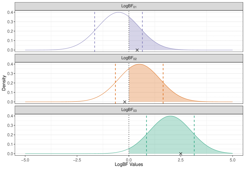
Figure 1: Illustrative example of the CBF procedure. The Log-BF distributions (purple: $\mathcal{H}_{1}\;\text{vs.}\;\mathcal{H}_{0}$, orange: $\mathcal{H}_{2}\;\text{vs.}\;\mathcal{H}_{0}$, green: $\mathcal{H}_{3}\;\text{vs.}\;\mathcal{H}_{0}$), the observed Log-BFs (crossed points) and HPDIs (dashed lines) are shown. The filled area after the zero threshold (dotted line) in each distribution represents the portion where the evidence for the alternative hypothesis is stronger than for the null hypothesis.

4 Simulation Studies

In this section, we assess the efficacy and applicability of the CBF approach through simulation studies. The simulations comprise three distinct studies, each focusing on different statistical distributions and their parameters. The main objective of each simulated study is to evaluate the effectiveness of the proposed method in selecting a well-balanced prior. This method aims to incorporate extensive past information when historical and current data are in agreement and to minimize this incorporation when there is a discrepancy between the two datasets. To assess this, we analyze a historical dataset and a series of current datasets that progressively diverge from it. Additionally, an expanded grid of hyperparameters for the Beta prior distribution is employed, ranging from $0.5$ to $6$ in increments of $0.5$. According to some sensitivity checks, each simulation study considers a $75\%$ HPDI threshold for the selection criterion in (8).

Firstly, let consider a specific discrete example for count data. Let $y_{0}=(y_{01},\ldots,y_{0N_{0}})$ and $y=(y_{1},\ldots,y_{N})$ denote the historical and current dataset, respectively. It is assumed that the datasets are generated from two different Poisson distributions, each characterized by rate parameters $\lambda_{0}$ for the historical data and $\lambda_{c}$ for the current data. Consequently, the BF is given by

$$\mathrm{BF}_{0,i}(y) =\dfrac{\int_{0}^{1}\mathrm{W}(\delta)\mathrm{Beta}(\delta\mid\eta_{i},\nu_{i})\mathrm{d}\delta}{\int_{0}^{1}\mathrm{W}(\delta)\mathrm{Beta}(\delta\mid 1,1)\mathrm{d}\delta},\;\;\;i=1,\ldots,M.$$

where

$$\mathrm{W}(\delta)=\dfrac{\left(\delta N_{0}+\beta_{0}\right)^{\delta N_{0}\overline{y}_{0}+\alpha_{0}}}{\Gamma(\delta N_{0}\overline{y}_{0})}\Gamma(N\overline{y}+\delta N_{0}\overline{y}_{0}+\alpha_{0})\mathrm{P}_{y}^{-1}\left[\left(N+\delta N_{0}+\beta_{0}\right)^{N\overline{y}+\delta N_{0}\overline{y}_{0}+\alpha_{0}}\right]^{-1},$$

with $\mathrm{P}_{y}=\prod_{j=1}^{N}y_{j}!$, $\overline{y}_{0}=\frac{1}{N_{0}}\sum_{h=1}^{N_{0}}y_{0h}$ and $\overline{y}=\frac{1}{N}\sum_{j=1}^{N}y_{j}$. For further details see Appendix A.

Figure 2 illustrates the evolution of the selected prior for $\delta$ in relation to the level of disagreement between the current and the historical studies. This disagreement is quantified by the difference between the historical rate parameter and the current rate parameter. The plot shows the median values of the selected prior for $\delta$ as points, with error bars indicating the first and third quartiles. Additionally, values in brackets indicate the selected hyperparameters chosen from the predefined grid. The plot highlights the procedure’s ability to select an appropriate prior according to the level of disagreement between the datasets. Specifically, as the disagreement increases, the selected prior shifts from a left-skewed Beta distribution – a $\mathrm{Beta}(5.5,0.5)$, suggesting a substantial incorporation of historical data (equal weight to the actual data), to a right-skewed Beta distribution – a $\mathrm{Beta}(0.5,6)$, implying a more conservative use of historical information.

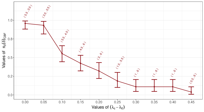
Figure 2: Poisson case. Shifts in the prior median (point) for the CBF derived prior for $\delta$, considering the 25th and 75th Percentiles (bar), in function of the difference between the current rate parameter $\lambda_{c}$ and the historical rate parameter $\lambda_{0}$. Above each interval, the couple of selected Beta hyperparameter are displayed.

The left panel of Figure 3 shows the mean and standard deviation (SD) of the marginal posterior distribution for the rate parameter $\lambda$, comparing two distinct scenarios. The first scenario employs the default $\mathrm{Beta}(1,1)$ as initial prior for $\delta$, while the second use the chosen Beta initial prior determined according to the selection criterion in (8). The comparison highlights that the posterior mean in both scenarios shows a similar increasing trend. This can be attributed to the progressive increase in the current rate parameter $\lambda_{c}$ which results in a greater discrepancy between current and historical data, leading to a higher discount of historical data. Furthermore, the marginal posterior distributions using the CBF selected prior are less diffused than those derived from the standard $\mathrm{Beta}(1,1)$ prior, leading to more precise results for $\lambda$. Specifically, when there is minimal disagreement between current and historical data, the posterior standard deviation for $\lambda$ is lower when using the CBF selected prior. As the disagreement increases, the difference between the standard deviations tends to reduce. Finally, when the disagreement is high, the posterior distribution under the CBF prior for $\delta$ remains less dispersed compared to the standard uniform prior.

The right panel of Figure 3 focuses on the posterior distribution for the weight parameter $\delta$, comparing the two previously described scenarios. When there is a low level of disagreement between the current and historical data, the CBF prior leads to posterior distributions that incorporate more historical information compared to the $\mathrm{Beta}(1,1)$ prior for $\delta$. Conversely, as the disagreement increases, the CBF prior becomes more conservative, discounting the historical data to a greater extent. Furthermore, the CBF prior consistently leads to more precise estimates with lower variability in the posterior distribution.

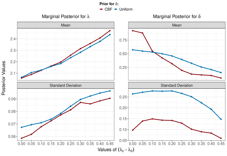
Figure 3: Poisson case. Mean and standard deviation (SD) of marginal posterior for $\lambda$ (left panel) and $\delta$ (right panel) using the the standard $\mathrm{Beta}(1,1)$ prior (blue squared lines) and the CBF derived Beta prior (red dotted lines).

A similar simulation study is conducted for the binomial model, which is frequently applied in medical contexts involving power priors. Let $N_{0}$ and $N$ denote the number of Bernoulli trials in the historical and current studies, respectively. Furthermore, let $y_{0}$ and $y$ represent the number of successes in these studies. Assuming a binomial likelihood with success probability $\theta$ for each study, and an initial Beta prior for both $\theta$ and the weight parameter $\delta$, the BF is

$$\mathrm{BF}_{0,i}(y)=\dfrac{\int_{0}^{1}\mathrm{BBin}(y\mid N,\delta y_{0}+p,\delta(N_{0}-y_{0})+q)\mathrm{Beta}\left(\delta\mid\eta_{i},\nu_{i}\right)\mathrm{d}\delta}{\int_{0}^{1}\mathrm{BBin}(y\mid N,\delta y_{0}+p,\delta(N_{0}-y_{0})+q)\mathrm{Beta}\left(\delta\mid 1,1\right)\mathrm{d}\delta},\;\;\;i=1,\ldots,M,$$

where $\mathrm{BBin}(\cdot\mid N,\alpha,\beta)$ is the beta-binomial discrete distribution. For further details see Appendix B.

Figure 4 shows the evolution of the selected prior for $\delta$ when analyzing a historical dataset followed by a series of current datasets. A $\mathrm{Beta}(1,1)$ is used as initial prior distribution for $\theta$, and the historical binomial likelihood presents a success probability of $0.2$. This simulation study demonstrates the proposed method’s ability to dynamically adapt the amount of historical information borrowed, based on the agreement between current and historical data. Specifically, when there is almost perfect agreement, the selected prior for $\delta$ is a $\mathrm{Beta}(6,0.5)$, indicating a higher level of historical information borrowing. As the level of agreement decreases, the prior for $\delta$ progressively shifts to $\mathrm{Beta}$ distributions that reduce the incorporation of historical data, reaching a $\mathrm{Beta}(0.5,6)$ distribution in cases of high disagreement.

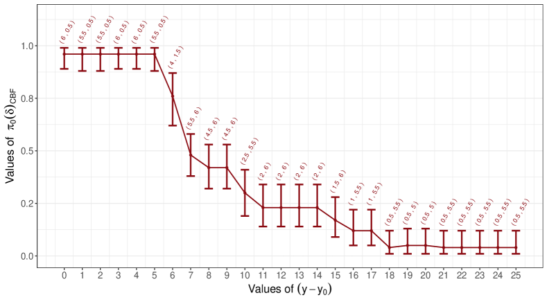
Figure 4: Binomial case. Shifts in the prior median (point) for the CBF derived prior for $\delta$, considering the 25th and 75th Percentiles (bar), in function of the difference between the current successes $y$ and the historical successes $y_{0}$. Above each interval, the couple of selected Beta hyperparameter are displayed.

Figure 5 shows the marginal posterior means and standard deviations for $\theta$ and $\delta$ comparing the uniform and CBF selected initial prior for the weight parameter. Particularly, the left panel of Figure 5 highlights that the CBF prior for $\delta$ results in marginal posterior distributions for $\theta$ that are generally more concentrated. This is particularly evident when there is either a low or high level of disagreement between current and historical data. Additionally, the posterior mean of $\theta$ follows a consistently similar trend when compared to the results obtained using the $\mathrm{Beta}(1,1)$ prior on $\delta$. Therefore, using the CBF prior leads to more accurate inferential conclusion in general.

The right panel of Figure 5 illustrates that when the discrepancy between historical and current data is minimal, the CBF prior for $\delta$ results in posterior distributions that incorporate a greater amount of historical information. As the discrepancy increases, the posterior distributions become more conservative, increasingly discounting the historical data. Furthermore, it is evident that the CBF prior for $\delta$ produces less diffused posterior distributions compared to those derived from a uniform prior.

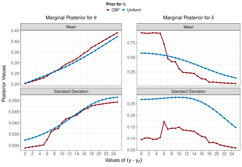
Figure 5: Binomial case. Mean and standard deviation (SD) of marginal posterior for $\theta$ (left panel) and $\delta$ (right panel) using the standard $\mathrm{Beta}(1,1)$ prior (blue squared lines) and the CBF derived Beta prior (red dotted lines).

Finally, we investigate a continuous response example commonly encountered in replication studies (Pawel et al., , 2024). A crucial question in this context is how effectively a replication (current) study has reproduced the results of an original (historical) study. Let $\mu$ be the unknown true effect size, with $\hat{\mu}_{s}$ representing the estimated effect size from study $s$, where $s\in\{o,r\}$ denotes “original” and “replication” studies, respectively. Furthermore, the effect size estimates are assumed to be normally distributed.

$$\hat{\mu}_{s}\mid\mu\sim\mathrm{N}\left(\mu,\sigma_{s}^{2}\right),$$

where $\sigma^{2}_{s}$ represents the variance of the estimated effect size $\hat{\mu}_{s}$, assumed to be known. The BF is given by

$$\mathrm{BF}_{0,i}(y) =\dfrac{\int_{0}^{1}\mathrm{N}\left(\hat{\mu}\mid\hat{\mu}_{o},\sigma^{2}+\sigma_{o}^{2}/\delta\right)\mathrm{Beta}\left(\delta\mid\eta_{i},\nu_{i}\right)\mathrm{d}\delta}{\int_{0}^{1}\mathrm{N}\left(\hat{\mu}\mid\hat{\mu}_{o},\sigma^{2}+\sigma_{o}^{2}/\delta\right)\mathrm{Beta}\left(\delta\mid 1,1\right)\mathrm{d}\delta},\;\;\;i=1,\ldots,M.$$

Further details are provided in Appendix C.

In Figure 6 is assumed that the effect size in the original study follows a normal distribution with mean $\mu_{o}=0$ and variance $\sigma^{2}_{o}=1$. We incrementally varied the true effect size of the replicated study in steps of 0.2, starting from a scenario of perfect agreement, where the replicated study’s effect size is $\mu_{r}=0$, and extending to scenarios of progressively greater disagreement, reaching a point where $\mu_{r}=6$. Our method effectively selected a well-balanced prior to address the plausible level of agreement between the original and replicated studies. Similar to the binomial case, a $\mathrm{Beta}(6,0.5)$ prior is chosen when the agreement is high. As the disagreement increases, the amount of borrowed information is progressively reduced, selecting the prior that most limits the incorporation of historical information – a $\mathrm{Beta}(0.5,6)$ – in cases of high disagreement.

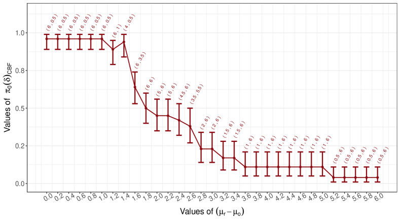
Figure 6: Gaussian case. Shifts in the prior median (point) for the CBF derived prior for $\delta$, considering the 25th and 75th Percentiles (bar), in function of the difference between the replicated study’s effect size $\mu_{r}$ and the original study’s effect size $\mu_{0}$. Above each interval, the couple of selected Beta hyperparameter are displayed.

Figure 7 shows that the CBF procedure effectively selects a prior for the weight parameter, reducing the standard deviation of the marginal posterior for $\mu$ compared to the $\mathrm{Beta}(1,1)$ prior, while maintaining a similar posterior mean for the effect size $\mu$. Additionally, similar results to those observed in previous simulation studies are obtained for the posterior distribution of $\delta$.

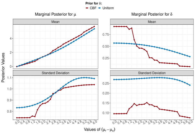
Figure 7: Gaussian case. Mean and standard deviation (SD) of marginal posterior for $\mu$ (left panel) and $\delta$ (right panel) using the standard $\mathrm{Beta}(1,1)$ prior (blue squared lines) and the CBF derived Beta prior (red dotted lines) for $\delta$.

5 Melanoma Clinical Trial

The efficacy of the CBF procedure on real data is evaluated through the analysis of two clinical trials. This analysis incorporates recent data from a new trial along with historical data from a previous study to assess earlier findings. Two melanoma trials conducted by the Eastern Cooperative Oncology Group (ECOG), specifically E2696 and E1694, are examined, involving 105 and 200 patients respectively. For further details see Kirkwood et al., 2001a ; Kirkwood et al., 2001b . These trials investigate the effects of interferon alfa-2b (IFN) treatment on patient survival rates. The E2696 trial assesses the efficacy of combining the GM2-KLH/QS-21 (GMK) vaccine with high-dose IFN therapy compared to the GMK vaccine alone in patients with resected high-risk melanoma. Furthermore, the E1694 trial evaluates the effectiveness of the GMK vaccine versus high-dose IFN therapy in a comparable group of patients. In conclusion, the findings from the E1694 trial corroborate earlier results from E2696, demonstrating that both intravenous and subcutaneous IFN can significantly reduce the relapse rate in melanoma patients. Figure 8 presents the survival curves from both trials, highlighting the beneficial impact of interferon treatment on patient survival.

Figure 8: Melanoma clinical trial. Survival Curves for E2696 and E1694 Trials. On the right, the end time survival probability for each treatment.

A Bayesian logistic regression model is applied to data from the E1694 trial and additional historical information from the E2696 trial is integrated using a normalized power prior as in (3). The analysis includes four additional covariates: age, sex, performance status, and treatment indicator. Parameter estimation is conducted using the probabilistic programming language Stan (Carpenter et al., , 2017) to perform Markov Chain Monte Carlo (MCMC) sampling via the rstan R package (Stan Development Team, , 2024). This involves four independent chains, each with 2000 iterations, discarding the first 1000 iterations as burn-in. To determine a well-balanced initial prior for the weight parameter using the CBF procedure, as described in Section 3.3, the bridge sampling approximation of the BF is employed via the bridgesampling R package (Gronau et al., , 2020). Furthermore, due to the lack of a closed-form expression for the normalizing constant in (4), the suggestion by van Rosmalen et al., (2018) to approximate the function $\log C(\delta)$ through linear interpolation is followed. Specifically, the grid-based approximation method proposed by Carvalho and Ibrahim, (2021) is used. This method involves defining a grid of points focused on areas where the derivative $C^{\prime}(\delta)$ is nearly zero, and employing a generalized additive model (GAM) for the linear interpolation step across a larger grid.

Initial priors for the coefficients of the four covariates are set using a weakly informative approach as outlined by Gelman et al., (2008). Specifically, a normal distribution with mean 0 and standard deviation 10 is assigned to each coefficient. Additionally, for the initial prior of the weight parameter, a $\mathrm{Beta}(5,0.5)$ is chosen based on the CBF procedure. This process involves a comprehensive evaluation of competing initial priors, considering a range of different Beta hyperparameters from 0.5 to 6 in increments of 0.5. Furthermore, a parallel processing strategy is employed to efficiently manage the computational effort required for this extensive hyperparameter exploration, ensuring streamlined and effective computational execution of the methodology.

Table 2 presents a comparison of posterior estimates for regression parameters under different initial Beta priors for $\delta$. These estimates include posterior means, standard deviations, and $95\%$ HPDIs. The priors compared are: the prior selected based on the CBF criterion described in (8), the standard uniform prior, the Jeffreys’ prior, and the $\mathrm{Beta}(2,2)$ prior. Notably, the well-balanced prior identified using the CBF procedure – a $\mathrm{Beta}(5,0.5)$ – results in consistently smaller posterior standard deviations for the treatment, sex, and performance status parameters compared to the other evaluated Beta priors, indicating more precise inferential conclusions. Additionally, the HPDIs for all the parameters of interest are narrower when using the prior from the CBF procedure. This suggests that, by incorporating a great amount of historical information, the CBF selected prior efficiently enhances the precision of the posterior parameter estimation.

Table 2: Melanoma clinical trial. Posterior mean, standard deviation (SD) and $95\%$ HPDI for the age, treatment, sex and performance status using different initial prior for the weight parameter.

$\pi_{0}(\delta)$	Parameter	Mean	SD	95$\%$ HPDI
Beta(5, 0.5)(1)	Age	0.015	0.010	(-0.004, 0.034)
	Treat.	-0.518	0.248	(-0.993, -0.029)
	Sex	-0.114	0.263	(-0.625, 0.382)
	Perf.	-0.472	0.346	(-1.142, 0.181)
Beta(1, 1)(2)	Age	0.014	0.010	(-0.006, 0.035)
	Treat.	-0.532	0.265	(-1.059, -0.022)
	Sex	-0.143	0.281	(-0.702, 0.388)
	Perf.	-0.478	0.372	(-1.212, 0.239)
Beta(0.5, 0.5)(3)	Age	0.015	0.010	(-0.004, 0.034)
	Treat.	-0.528	0.261	(-1.023, -0.022)
	Sex	-0.120	0.269	(-0.664, 0.369)
	Perf.	-0.471	0.351	(-1.172, 0.204)
Beta(2, 2)	Age	0.014	0.010	(-0.005, 0.036)
	Treat.	-0.542	0.271	(-1.078, -0.012)
	Sex	-0.148	0.273	(-0.678, 0.381)
	Perf.	-0.490	0.376	(-1.216, 0.219)

⁽¹⁾CBF ⁽²⁾Uniform ⁽³⁾Jeffreys

Figure 9 further emphasizes this result by showing the marginal posterior distribution for the four parameters of interest with their corresponding $95\%$ HPDI comparing the prior derived from the CBF procedure and the conventional $\mathrm{Beta}(1,1)$ prior.

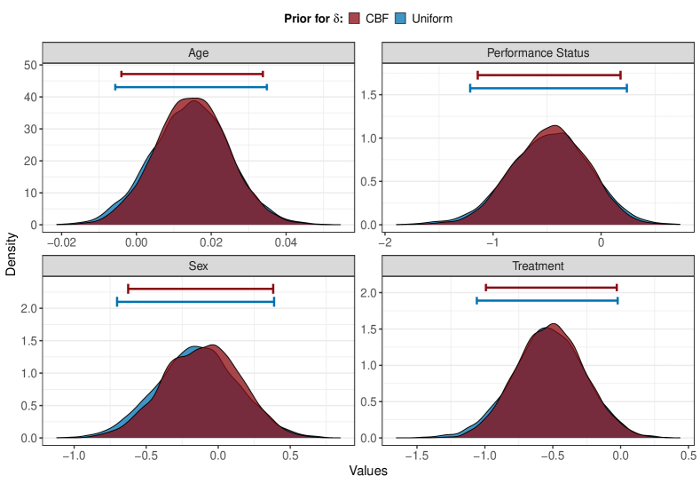
Figure 9: Melanoma clinical trial. Marginal posterior densities for the age, performance status, sex and treatment indicator. The horizontal error bars represent the corresponding $95\%$ highest posterior density interval.

6 Discussion

The power prior method presents a flexible way to construct an informative prior by combining a prior distribution with the weighted likelihood of previous data. This combined posterior then serves as the prior for new studies. However, determining the appropriate weight parameter presents a significant challenge, whether it is fixed or its prior distribution is being evaluated. While several methods exist for setting a fixed weight parameter, fully Bayesian approaches for eliciting more informative priors are not usually addressed in the related literature.

Gravestock and Held, (2017) highlighted that while the fully Bayesian approach is inherently flexible, it may not sufficiently address the disagreements between historical and current data. This issue frequently stems from the default use of a non-informative prior, which might not be sensitive enough to detect significant divergences. Consequently, we advocate for the use of a more informative prior specifically designed to detect potential conflict between historical and current datasets, improving the robustness of the resulting statistical inferences.

Our proposed CBF procedure is a novel response to this challenge. It seeks to select a more informative prior than the conventional non-informative one by utilizing hypothetical replications derived from the posterior predictive distribution. The selected prior has minimal influence on the posterior central summary statistics while simultaneously achieving a smaller posterior variance for the parameters of interest. The efficacy of this approach is demonstrated through both simulation studies and the application to melanoma data, proving its robustness and effectiveness in distinguishing between different prior specifications. The ability of this method to select a well-balanced prior based on the agreement between historical and current data, as evidenced in the melanoma study, emphasizes its practical relevance in real-world applications.

A crucial aspect of our CBF procedure is the choice of the HPDI for assessing the placement of the observed Log-BF within the distribution of replicated Log-BFs. This decision is crucial as it directly influences the interpretation of empirical evidence relative to the modeled hypotheses. A narrower HPDI is recommended when the aim is to limit the range of acceptable values, thereby enhancing the strength and reliability of empirical findings. Future research will focus on developing quantitative methods for determining the appropriate HPDI width.

The methodology presented in this paper offers several areas for potential improvement. Firstly, the selection criteria outlined in (8) could be refined to more effectively identify well-calibrated priors, particularly in cases of moderate agreement between historical and current data. Additionally, to reduce computational time, it is advisable to consider alternatives to the grid search method employed in this study. Instead of exhaustively exploring all hyperparameters within the grid, methods that target a relevant subset of the parameter space should be explored. Furthermore, future work should focus on providing a more comprehensive analysis of the theoretical properties of the CBF method.

Finally, a thorough comparison with the optimal prior proposal by Shen (2023) and methods that provide an estimate for $\delta$, possibly in terms of MSE or other measures, possibly using measures such as MSE or other relevant metrics, is a primary goal for future research.

Software and Data Availability

All analyses were conducted in the R programming language version $4.2.3$ (R Core Team, , 2023). The code and data to reproduce this manuscript are openly available at https://github.com/RoMaD-96/CBFpp.

Appendix A Poisson with unknown rate parameter $\lambda$

Let $y_{0}=(y_{01},\ldots,y_{0N_{0}})$ denote a historical dataset, which is presumed to originate from a Poisson distribution characterized by a rate parameter $\lambda_{0}=2$. In this simulation, we adopt the conjugate prior approach, wherein:

$$\lambda \sim\mathrm{Gamma}(\alpha_{0},\beta_{0}),$$

$$y_{0}\mid\lambda \sim\mathrm{Poisson}(\lambda).$$

Notably, the hyperparameters of the Gamma initial prior are set to $\alpha_{0}=\beta_{0}=1$. Moreover, the normalized power prior is

$$\pi\left(\lambda,\delta\mid y_{0}\right) =\mathrm{Gamma}\left(\lambda\mid\delta N_{0}\overline{y}_{0}+\alpha_{0},\delta N_{0}+\beta_{0}\right)\mathrm{Beta}(\delta\mid\eta,\nu),$$ (9)

where $\overline{y}_{0}=\frac{1}{N_{0}}\sum_{h=1}^{N_{0}}y_{0h}$. Combining (9) with the likelihood of the current data yields to the following joint posterior for $(\lambda,\delta)$

$$\pi(\lambda,\delta\mid y_{0},y) =\dfrac{L(\lambda\mid y)\pi(\lambda,\delta\mid y_{0})}{\int_{0}^{1}\int_{0}^{+\infty}L(\lambda\mid y)\pi(\lambda,\delta\mid y_{0})\mathrm{d}\lambda\mathrm{d}\delta}$$

$$=\dfrac{\mathrm{Poisson}(y\mid\lambda)\mathrm{Gamma}\left(\lambda\mid\delta N_{0}\overline{y}_{0}+\alpha_{0},\delta N_{0}+\beta_{0}\right)\mathrm{Beta}(\delta\mid\eta,\nu)}{\int_{0}^{1}\mathrm{W}(\delta)\mathrm{Beta}(\delta\mid\eta,\nu)\mathrm{d}\delta}$$

where

$$\mathrm{W}(\delta)=\dfrac{\left(\delta N_{0}+\beta_{0}\right)^{\delta N_{0}\overline{y}_{0}+\alpha_{0}}}{\Gamma(\delta N_{0}\overline{y}_{0})}\Gamma(N\overline{y}+\delta N_{0}\overline{y}_{0}+\alpha_{0})\mathrm{P}_{y}^{-1}\left[\left(N+\delta N_{0}+\beta_{0}\right)^{N\overline{y}+\delta N_{0}\overline{y}_{0}+\alpha_{0}}\right]^{-1},$$

with $\mathrm{P}_{y}=\prod_{j=1}^{N}y_{j}!$ and $\overline{y}=\frac{1}{N}\sum_{j=1}^{N}y_{j}$. Moreover, the BF is

$$\mathrm{BF}_{0,i}(y) =\dfrac{\int_{0}^{1}\mathrm{W}(\delta)\mathrm{Beta}(\delta\mid\eta_{i},\nu_{i})\mathrm{d}\delta}{\int_{0}^{1}\mathrm{W}(\delta)\mathrm{Beta}(\delta\mid 1,1)\mathrm{d}\delta},\;\;\;i=1,\ldots,M.$$

Appendix B Binomial with unknown success probability $\theta$

Let $N_{0}$ and $N$ denote the number of Bernoulli trials in the historical and current studies, respectively. The terms $y_{0}$ and $y$ represent the successes in these studies. Assuming a binomial likelihood with a success probability $\theta$ for each study and an initial Beta prior for both $\theta$ and the weight parameter $\delta$, the normalized power prior is

$$\pi(\theta,\delta\mid y_{0}) =\dfrac{\left[\mathrm{Bin}(y_{0}\mid\theta,N_{0})\right]^{\delta}\mathrm{Beta}(\theta\mid p,q)\mathrm{Beta}(\delta\mid\eta,\nu)}{\int_{0}^{1}\left[\mathrm{Bin}(y_{0}\mid\theta,N_{0})\right]^{\delta}\mathrm{Beta}(\theta\mid p,q)\mathrm{d}\theta}$$

$$=\mathrm{Beta}\left(\theta\mid\delta y_{0}+p,\delta\left(N_{0}-y_{0}\right)+q\right)\mathrm{Beta}(\delta\mid\eta,\nu).$$

In light of the current data the posterior distribution is

$$\pi\left(\theta,\delta\mid y,y_{0}\right) =\frac{L(\theta\mid y)\pi\left(\theta,\delta\mid y_{0}\right)}{\int_{0}^{1}\int_{0}^{1}L\left(\theta\mid y\right)\pi\left(\theta,\delta\mid y_{0}\right)\mathrm{d}\theta\mathrm{d}\delta}$$

$$=\dfrac{\mathrm{Bin}\left(y\mid\theta,N\right)\mathrm{Beta}\left(\theta\mid\delta y_{0}+p,\delta\left(N_{0}-y_{0}\right)+q\right)\mathrm{Beta}(\delta\mid\eta,\nu)}{\int_{0}^{1}\mathrm{BBin}(y\mid N,\delta y_{0}+p,\delta(N_{0}-y_{0})+q)\mathrm{Beta}(\delta\mid\eta,\nu)\mathrm{d}\delta},$$

where $\mathrm{BBin}(\cdot\mid N,\alpha,\beta)$ is the beta-binomial discrete distribution. Therefore, the BF is

$$\mathrm{BF}_{0,i}(y) =\dfrac{\int_{0}^{1}\mathrm{BBin}(y\mid N,\delta y_{0}+p,\delta(N_{0}-y_{0})+q)\mathrm{Beta}\left(\delta\mid\eta_{i},\nu_{i}\right)\mathrm{d}\delta}{\int_{0}^{1}\mathrm{BBin}(y\mid N,\delta y_{0}+p,\delta(N_{0}-y_{0})+q)\mathrm{Beta}\left(\delta\mid 1,1\right)\mathrm{d}\delta},\;\;\;i=1,\ldots,M.$$

Appendix C Gaussian with unknown mean $\mu$

Let $\mu$ be the unknown true effect size, with $\hat{\mu}_{s}$ representing the estimated effect size from study $s$, where $s\in\{o,r\}$ denotes “original” and “replication” studies, respectively. Furthermore, we assume that the effect size estimates are normally distributed.

$$\hat{\mu}_{s}\mid\mu\sim\mathrm{N}\left(\mu,\sigma_{s}^{2}\right),$$

where $\sigma^{2}_{s}$ represents the variance of the estimated effect size $\hat{\mu}_{s}$, assumed to be known. Let consider an initial improper prior for the effect size parameter $\pi_{0}(\mu)\propto 1$ and a Beta prior for the weight parameter $\delta$ then the normalized power prior is

$$\pi\left(\mu,\delta\mid y_{o}\right) =\mathrm{N}\left(\mu\mid\hat{\mu}_{o},\dfrac{\sigma_{o}^{2}}{\delta}\right)\mathrm{Beta}(\delta\mid\eta,\nu).$$

Updating the previous prior with the likelihood of the replicated data yields to the following posterior distribution

$$\pi\left(\mu,\delta\mid y,y_{o}\right) =\frac{L(\mu\mid y)\pi\left(\mu,\delta\mid y_{o}\right)}{\int_{0}^{1}\int_{-\infty}^{\infty}L\left(\mu\mid y\right)\pi\left(\mu,\delta\mid y_{o}\right)\mathrm{d}\mu\mathrm{d}\delta}$$

$$=\dfrac{\mathrm{N}\left(\hat{\mu}\mid\mu,\sigma^{2}\right)\mathrm{N}\left(\mu\mid\hat{\mu}_{o},\sigma_{o}^{2}/\delta\right)\mathrm{Beta}(\delta\mid\eta,\nu)}{\int_{0}^{1}\mathrm{N}\left(\hat{\mu}\mid\hat{\mu}_{o},\sigma^{2}+\sigma_{o}^{2}/\delta\right)\mathrm{Beta}\left(\delta\mid\eta,\nu\right)\mathrm{d}\delta}.$$

Furthermore, the BF is

$$\mathrm{BF}_{0,i}(y) =\dfrac{\int_{0}^{1}\mathrm{N}\left(\hat{\mu}\mid\hat{\mu}_{o},\sigma^{2}+\sigma_{o}^{2}/\delta\right)\mathrm{Beta}\left(\delta\mid\eta_{i},\nu_{i}\right)\mathrm{d}\delta}{\int_{0}^{1}\mathrm{N}\left(\hat{\mu}\mid\hat{\mu}_{o},\sigma^{2}+\sigma_{o}^{2}/\delta\right)\mathrm{Beta}\left(\delta\mid 1,1\right)\mathrm{d}\delta},\;\;\;i=1,\ldots,M.$$

References

- Bennett et al., (2021) Bennett, M., White, S., Best, N., and Mander, A. (2021). A novel equivalence probability weighted power prior for using historical control data in an adaptive clinical trial design: A comparison to standard methods. Pharmaceutical Statistics, 20(3):462–484.
- Carpenter et al., (2017) Carpenter, B., Gelman, A., Hoffman, M. D., Lee, D., Goodrich, B., Betancourt, M., Brubaker, M., Guo, J., Li, P., and Riddell, A. (2017). Stan: A probabilistic programming language. Journal of Statistical Software, 76(1):1–32.
- Carvalho and Ibrahim, (2021) Carvalho, L. M. and Ibrahim, J. G. (2021). On the normalized power prior. Statistics in Medicine, 40(24):5251–5275.
- Chen and Ibrahim, (2000) Chen, M.-H. and Ibrahim, J. G. (2000). Power prior distributions for regression models. Statistical Science, 15(1):46 – 60.
- Chen and Ibrahim, (2006) Chen, M.-H. and Ibrahim, J. G. (2006). The relationship between the power prior and hierarchical models. Bayesian Analysis, 1(3):551–574.
- Chen et al., (2000) Chen, M.-H., Ibrahim, J. G., and Shao, Q.-M. (2000). Power prior distributions for generalized linear models. Journal of Statistical Planning and Inference, 84(1-2):121–137.
- Cook et al., (2006) Cook, S., Gelman, A., and Rubin, D. B. (2006). Validation of software for Bayesian models using posterior quantiles. Journal of Computational and Graphical Statistics, 15(3):675–692.
- De Santis, (2006) De Santis, F. (2006). Power priors and their use in clinical trials. The American Statistician, 60(2):122–129.
- Dickey and Lientz, (1970) Dickey, J. M. and Lientz, B. P. (1970). The weighted likelihood ratio, sharp hypotheses about chances, the order of a Markov chain. The Annals of Mathematical Statistics, 41(1):214–226.
- Duan et al., (2006) Duan, Y., Ye, K., and Smith, E. P. (2006). Evaluating water quality using power priors to incorporate historical information. Environmetrics, 17(1):95–106.
- Egidi et al., (2022) Egidi, L., Pauli, F., and Torelli, N. (2022). Avoiding prior–data conflict in regression models via mixture priors. Canadian Journal of Statistics, 50(2):491–510.
- Evans and Moshonov, (2006) Evans, M. and Moshonov, H. (2006). Checking for prior-data conflict. Bayesian Analysis, 1(4):893 – 914.
- Garcia-Donato and Chen, (2005) Garcia-Donato, G. and Chen, M.-H. (2005). Calibrating Bayes factor under prior predictive distributions. Statistica Sinica, 15(2):359–380.
- Gelman et al., (2008) Gelman, A., Jakulin, A., Pittau, M. G., and Su, Y.-S. (2008). A weakly informative default prior distribution for logistic and other regression models. The Annals of Applied Statistics, 2(4):1360 – 1383.
- Gelman et al., (2020) Gelman, A., Vehtari, A., Simpson, D., Margossian, C. C., Carpenter, B., Yao, Y., Kennedy, L., Gabry, J., Bürkner, P.-C., and Modrák, M. (2020). Bayesian workflow. arXiv preprint arXiv:2011.01808.
- Geweke, (2004) Geweke, J. (2004). Getting it right: Joint distribution tests of posterior simulators. Journal of the American Statistical Association, 99(467):799–804.