Theory of superconductivity in twisted transition metal dichalcogenide homobilayers
Abstract
For the first time, robust superconductivity has been independently observed in twisted WSe2 bilayers by two separate groups [Y. Xia et al., arXiv:2405.14784; Y. Guo et al., arXiv:2406.03418.]. In light of this, we explore the possibility of a universal superconducting pairing mechanism in twisted WSe2 bilayers. Using a continuum band structure model and a phenomenological boson-mediated effective electron-electron attraction, we find that intervalley intralayer pairing predominates over interlayer pairing. Notably, despite different experimental conditions, both twisted WSe2 samples exhibit a comparable effective attraction strength. This consistency suggests that the dominant pairing glue is likely independent of the twist angle and layer polarization, pointing to a universal underlying boson-induced pairing mechanism.
Introduction— The emergence of moiré superlattice in twisted transition metal dichalcogenide (TMD) homobilayers has led to the observation of a rich set of strongly correlated phases Tang et al. (2020); Regan et al. (2020); Xu et al. (2020); Wang et al. (2020a); Li et al. (2021a); Ghiotto et al. (2021); Li et al. (2021b); Foutty et al. (2024); Cai et al. (2023); Zeng et al. (2023); Park et al. (2023); Xu et al. (2023), from correlated insulators at integer fillings to fractional Chern insulators in the absence of an external magnetic field. While the phases driven by strong electron-electron interaction manifest in the moiré TMD bilayers, robust observable superconductivity (SC) at dilute doping densities–associated with a few carriers per moiré unit cell–has remained elusive in most moiré TMD systems Wang et al. (2020b). On the other hand, both moiré and moiréless graphene multilayers have demonstrated reproducible SC with ranging from mK to K Cao et al. (2018); Yankowitz et al. (2019); Lu et al. (2019); Park et al. (2021); Hao et al. (2021); Cao et al. (2021); Oh et al. (2021); Zhou et al. (2021, 2022); Su et al. (2023); Zhang et al. (2023); Holleis et al. ; Li et al. (2024), indicating that SC is a generic feature in graphene-based multilayers. The source of such a striking difference between moiré TMD and moiré graphene systems is an important unsolved puzzle in condensed matter and material physics.
Recently, two groups have independently discovered robust SC in twisted WSe2 bilayers (tWSe2). One group reported SC at a filling factor with a twist angle of and a small displacement field Xia et al. . The critical temperature was estimated to be K. The other group observed SC around with a twist angle of and a large displacement field Guo et al. . The critical temperature was approximately K. We will refer to these two experimental samples as Sample A and Sample B, respectively, throughout our paper.
In this Letter, we investigate SC in tWSe2 using a realistic continuum band structure model and a phenomenological boson-mediated BCS model without assuming a specific pairing mechanism. We demonstrate the dominance of intervalley intralayer pairing with an order parameter consistent with a mixture of and waves Chou et al. (2022a); Zegrodnik and Biborski (2023); Akbar et al. . Our estimates of the effective coupling constants of SC in two different experiments show very similar values, suggesting a universal dominant pairing mechanism in tWSe2 (i.e., the same bosonic glue). The possible microscopic mechanisms and the importance of the in-plane magnetic field response are also discussed. Our work represents the first systematic investigation of the SC phenomenology in tWSe2 systems, paving the way for future exploration of SC in moiré TMD systems.
Band Structure Model— Our phenomenological superconducting mean-field theory is based on the low-energy continuum model of tWSe2 Wu et al. (2019a), of which the valley-projected Hamiltonian is
| (1) |
where is the effective mass approximation of the valence band edge at the Dirac point of layer . is the momentum measured from the Dirac points, and is the interlayer energy difference due to the displacement field. The layer-dependent moiré potential and the interlayer tunneling are spatially periodic with moiré periodicity,
| (2) | |||
| (3) |
, are the first-shell moiré reciprocal lattice vectors, with as the length of moiré primitive reciprocal lattice vector. In the calculations throughout this paper, we use the continuum model parameters fitted by large-scale DFT calculations Devakul et al. (2021): meV, , meV, lattice constant , and the effective mass with being the electron mass.
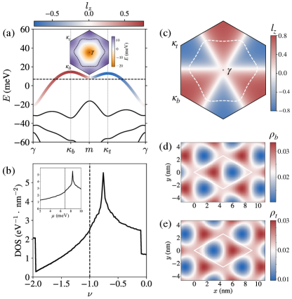
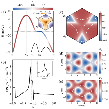
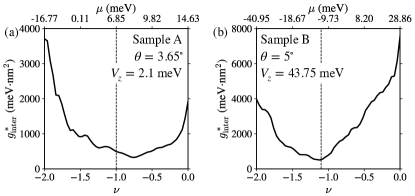
Figures 1 and 2 show the moiré band structures, density of states (DOS) and layer polarization in momentum and real space for Samples A and B. The layer polarization operator is represented by the Pauli matrix acting on the layer subspace. In Sample A, the layer is weakly polarized due to the small displacement field, corresponding to an interlayer energy difference of approximately meV Xia et al. ; Wef . In momentum space, as shown in Fig. 1(c), the wave function is localized on each layer around its Dirac point. In real space, depicted in Fig. 1(d-e), the layer projected density forms two triangular lattices centered on XM or MX local stackings, creating an effective honeycomb lattice with a small onsite energy difference. The DOS plot in Fig. 1(b) shows a Van Hove singularity (VHS) around . The SC observed at is only meV away from the VHS (inset of Fig. 1(b)). In our notation, the filling factor represents the number of electrons per moiré unit cell. In Sample B, a large displacement field induces an interlayer energy difference of meV Guo et al. ; Wea , resulting in strong layer polarization (Fig. 2(c-e)). The VHS is located at (Fig. 2(b)), which is less than meV away from the chemical potential at the filling factor , where SC was observed. This proximity is conducive to pairing instability.
Despite the significant differences in band structure, layer polarization, and effective lattice model between Samples A and B, we explore the possibility that the same underlying mechanism is responsible for SC in both cases in the next section.
Superconductivity— Closely connected to the two experiments, we study the effective pairing strength in Samples A and B using a phenomenological BCS theory without assuming a specific pairing mechansim. We will discuss the possible pairing glues, e.g., phonons and magnons, at the end of this Letter. Given that no evidence of time-reversal symmetry (TRS) breaking was observed near the superconducting phase in either sample, we consider only the intervalley pairing that preserves TRS. In the following part, we focus on intralayer pairing, as detailed in Appendix A, the interlayer pairing is significantly weaker by a factor of five to ten. The dominance of the intralayer pairing is a direct consequence of the layer polarization patterns as shown in Figs. 1(c) and 2(c).
The effective electron-electron attraction mediated by intralayer bosons is given by
| (4) |
where is the system area, and we approximate the intervalley intralayer pairing strength by a tunable static and momentum independent potential . The density operator, , is defined as
| (5) |
where is the valley index, represents the layer degree of freedom and is in the first moiré Brillouin zone (MBZ). Thus, the effective attraction Eq. (4) is
| (6) |
The factor of 2 in Eq. (4) is canceled by summing over valleys and keeping only the intervalley terms. Projecting to the first moiré valence band of tWSe2, the effective pairing Hamiltonian becomes
| (7) | |||
| (8) |
where () is the quasiparticle creation (annihilation) operator in the plane-wave expansion,
| (9) |
with and being the moiré reciprocal lattice vectors.
For , the linearized gap equation in the BCS mean-field approximation is
| (10) |
is the quasiparticle eigenenergy of the first moiré valence band and is the chemical potential. In obtaining Eq. (8) and (10), we have used the time-reversal symmetry properties
| (11) | |||
| (12) |
Equation (10) can be rewritten in the matrix form:
| (13) |
At the critical point , Eq. (13) has only one stable solution. Given the electron-boson coupling strength , is found by obtaining the largest eigenvalue of to be . Equivalently, for a given temperature , the critical electron-boson coupling strength is the inverse of the maximum eigenvalue of .
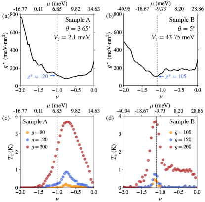
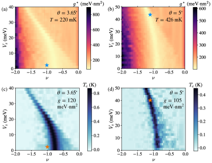
In Fig. 3(a-b), we show as a function of filling factor for Sample A, given the experimental K, and for Sample B, given the experimental K. reaches its minimum at the VHS for both samples, around for Sample A (Fig. 1(b)) and for Sample B (Fig. 2(b)). The minimum is approximately () meVnm2 for Sample A (B). At the filling factor where robust SC was observed, meVnm2 (at ) for Sample A, and meVnm2 (at ) for Sample B. The similar values of in the two very different samples strongly suggest intralayer pairing with a universal bosonic glue producing SC. We note that the interlayer pairing plays a minor role in this system, as detailed in Appendix B, the corresponding electron-boson coupling strength is at least five times larger than the intralayer for Sample A and ten times larger for Sample B.
In Fig 3(c-d), is shown as a function of for several representative values of . In both samples, reaches its maximum at the VHS and remains observable away from the VHS, similar to the situation found in the graphene multilayers Löthman and Black-Schaffer (2017); Chou et al. (2021, 2022b, 2022c). We note that non-adiabatic vertex corrections Cappelluti and Pietronero (1996); Phan and Chubukov (2020), which we ignore, might become important for doping densities very close to VHS. This is an interesting subject for future work. To further explore the dependence of and on the displacement field, which is a common experimental tuning parameter, we show phase diagrams of and in Appendix B for twist angles and . In both cases, the minimum and maximum track the VHS.
For , the order parameter is solved self-consistently,
| (14) |
where . At , the hyperbolic tangent term simplifies to 1.
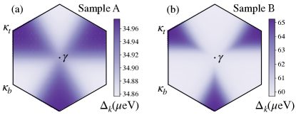
The -space distributions of the order parameters for Samples A and B, calculated at , are shown in Fig. 4. Since we consider only intralayer pairing, the symmetry of closely matches that of the layer polarization shown in Fig. 1(c) and Fig. 2(c), indicating a mixture of and waves Zegrodnik and Biborski (2023); Akbar et al. . In Sample A, , and in Sample B, where is the -space average of . Both ratios are close to the BCS mean-field value of .
Discussion— We develop a BCS theory for the recently observed SC in tWSe2. We establish that the SC likely arises from the same bosonic glue in two different experiments with different twist angles, displacement fields, and doping levels. The dominant pairing is intervalley intralayer interaction with an order parameter symmetry, and the maximum is not far from the VHS. Take the acoustic phonon as an example Wu et al. (2019b); Wu and Das Sarma (2020); Lewandowski et al. (2021); Chou et al. (2021, 2022b, 2022c); Boström et al. for the bosonic glue, the calculated is related to the deformation potential by . Using the mass density g/cm2 and sound velocity cm/s of monolayer WSe2 Jin et al. (2014), of Samples A and B in Fig. 3(a-b) correspond to deformation potentials of eV and eV, respectively, which are in the same order of magnitude as eV for monolayer WSe2 estimated from previous density functional theory (DFT) calculations Jin et al. (2014). The quantitative extraction of the deformation potential is difficult and DFT estimates are often much smaller than experimental values, a common occurrence in semiconductors.
It is also possible that the SC observed in both samples is mediated by magnons, as suggested by the close proximity of the SC to the correlated state, very likely of an antiferromagnetic order, and the that peaks near the phase boundary between these states. Understanding the magnetic order is essential for characterizing the nature of spin fluctuations and the resulting superconducting state. At present, the underlying mechanism of SC remains an unresolved and intriguing question that future experimental and theoretical work should address.
Next, we comment on the role of Coulomb interactions. Coulomb interactions may result in correlated states Kim et al. that could preempt SC predicted by our phenomenological BCS theory. Moreover, the band renormalization effect, which we ignore, may quantitatively adjust the single-particle band structure used in this Letter. The Coulomb repulsion in the Cooper channel is effectively captured by our theory through the effective coupling constant . Microscopic calculations incorporating the frequency-dependent pairing and Coulomb interactions are necessary for quantitative understanding of the underlying SC mechanism in tWSe2 Xia et al. ; Guo et al. .
Finally, we discuss the response to an in-plane magnetic field, which has been an important tool to discern the properties of SC in graphene-based materials Cao et al. (2021); Zhou et al. (2021, 2022); Su et al. (2023); Zhang et al. (2023); Holleis et al. ; Li et al. (2024). In WSe2, the Zeeman effect can be ignored due to large Ising spin-orbit coupling. However, the orbital effect might still be nontrivial as the separation between two WSe2 layers is not small. We find that SC is suppressed by an in-plane magnetic field of a few Teslas because the nesting of intervalley pairing requires , which is easily violated in the presence of a magnetic field. Additionally, an in-plane magnetic field may influence nearby correlated states; for example, in an antiferromagnetic state, spin fluctuation can be reduced by an applied magnetic field, weakening fluctuation-induced pairing. Systematic investigations along these lines are essential for understanding SC in tWSe2.
Acknowledgments— We thank Yuting Tan for useful discussions. Y.-Z. C. and J. Z. also acknowledge useful conversation with Yi Huang and Jay D. Sau. This work is supported by the Laboratory for Physical Sciences.
Appendix A Supplementary Information
Appendix B A. The Interlayer pairing
Similar to the derivation of intralayer pairing in the main text, the effective electron-electron attraction mediated by interlayer pairing is
| (15) |
where represents the opposite layer of . The corresponding pairing Hamiltonian and effective coupling are
| (16) | |||
| (17) |
Similar to Fig. 3(a-b), the critical electron-boson coupling strength for interlayer pairing is shown in Fig. 5. For Sample A, as a function of exhibits a similar trend to the obtained from intralayer pairing (Fig. 3(a)), but is scaled up by a factor of . This is because the layer-projected wave function is localized in separate regions in -space, as shown in Fig. 1(c), and the layer polarization has a weak dependence on due to the small displacement field. For Sample B, however, is much larger than the intralayer pairing (Fig. 3(b)) at small filling , because interlayer pairing is weaker for larger layer polarization. In Sample B, the interlayer pairing strength is at least ten times weaker than that of the intralayer pairing.
Appendix C B. Superconductivity phase diagram
To further explore the superconducting properties, we show the phase diagrams of and across a broad range of displacement fields (or equivalently interlayer energy difference ) and filling factors for twist angles and in Fig. 6, in which the conditions for experimentally realized SC in Samples A and B are marked by stars. In both cases, the minimum and maximum track the VHS. Remarkably, over the broad parameter space, values are similar in both samples (Fig. 6(a-b)) with different twist angles. For the smaller twist angle (Fig. 6(a,c)), is maximized at for a small displacement field, and at for an intermediate displacement field, followed by a decrease in with increasing . For the larger twist angle (Fig. 6(b,d)), the VHS is pinned near , as well as maximum . In Fig. 6(d), the maximum remains nearly constant with varying within the parameter range in our calculations. Note that the difference in maximum between Fig. 6(c) and (d) results from the different values used in these figures.
References
- Tang et al. (2020) Y. Tang, L. Li, T. Li, Y. Xu, S. Liu, K. Barmak, K. Watanabe, T. Taniguchi, A. H. MacDonald, J. Shan, and K. F. Mak, Nature 579, 353 (2020).
- Regan et al. (2020) E. C. Regan, D. Wang, C. Jin, M. I. B. Utama, B. Gao, X. Wei, S. Zhao, W. Zhao, Z. Zhang, K. Yumigeta, M. Blei, J. D. Carlström, K. Watanabe, T. Taniguchi, S. Tongay, M. Crommie, A. Zettl, and F. Wang, Nature 579, 359 (2020).
- Xu et al. (2020) Y. Xu, S. Liu, D. A. Rhodes, K. Watanabe, T. Taniguchi, J. Hone, V. Elser, K. F. Mak, and J. Shan, Nature 587, 214 (2020).
- Wang et al. (2020a) L. Wang, E.-M. Shih, A. Ghiotto, L. Xian, D. A. Rhodes, C. Tan, M. Claassen, D. M. Kennes, Y. Bai, B. Kim, K. Watanabe, T. Taniguchi, X. Zhu, J. Hone, A. Rubio, A. N. Pasupathy, and C. R. Dean, Nature Materials 19, 861 (2020a).
- Li et al. (2021a) T. Li, S. Jiang, L. Li, Y. Zhang, K. Kang, J. Zhu, K. Watanabe, T. Taniguchi, D. Chowdhury, L. Fu, J. Shan, and K. F. Mak, Nature 597, 350 (2021a).
- Ghiotto et al. (2021) A. Ghiotto, E.-M. Shih, G. S. S. G. Pereira, D. A. Rhodes, B. Kim, J. Zang, A. J. Millis, K. Watanabe, T. Taniguchi, J. C. Hone, L. Wang, C. R. Dean, and A. N. Pasupathy, Nature 597, 345 (2021).
- Li et al. (2021b) T. Li, S. Jiang, B. Shen, Y. Zhang, L. Li, Z. Tao, T. Devakul, K. Watanabe, T. Taniguchi, L. Fu, J. Shan, and K. F. Mak, Nature 600, 641 (2021b).
- Foutty et al. (2024) B. A. Foutty, C. R. Kometter, T. Devakul, A. P. Reddy, K. Watanabe, T. Taniguchi, L. Fu, and B. E. Feldman, Science 384, 343 (2024).
- Cai et al. (2023) J. Cai, E. Anderson, C. Wang, X. Zhang, X. Liu, W. Holtzmann, Y. Zhang, F. Fan, T. Taniguchi, K. Watanabe, Y. Ran, T. Cao, L. Fu, D. Xiao, W. Yao, and X. Xu, Nature 622, 63 (2023).
- Zeng et al. (2023) Y. Zeng, Z. Xia, K. Kang, J. Zhu, P. Knüppel, C. Vaswani, K. Watanabe, T. Taniguchi, K. F. Mak, and J. Shan, Nature 622, 69 (2023).
- Park et al. (2023) H. Park, J. Cai, E. Anderson, Y. Zhang, J. Zhu, X. Liu, C. Wang, W. Holtzmann, C. Hu, Z. Liu, T. Taniguchi, K. Watanabe, J.-H. Chu, T. Cao, L. Fu, W. Yao, C.-Z. Chang, D. Cobden, D. Xiao, and X. Xu, Nature 622, 74 (2023).
- Xu et al. (2023) F. Xu, Z. Sun, T. Jia, C. Liu, C. Xu, C. Li, Y. Gu, K. Watanabe, T. Taniguchi, B. Tong, J. Jia, Z. Shi, S. Jiang, Y. Zhang, X. Liu, and T. Li, Phys. Rev. X 13, 031037 (2023).
- Wang et al. (2020b) L. Wang, E.-M. Shih, A. Ghiotto, L. Xian, D. A. Rhodes, C. Tan, M. Claassen, D. M. Kennes, Y. Bai, B. Kim, K. Watanabe, T. Taniguchi, X. Zhu, J. Hone, A. Rubio, A. N. Pasupathy, and C. R. Dean, Nature Materials 19, 861 (2020b).
- Cao et al. (2018) Y. Cao, V. Fatemi, S. Fang, K. Watanabe, T. Taniguchi, E. Kaxiras, and P. Jarillo-Herrero, Nature 556, 43 (2018).
- Yankowitz et al. (2019) M. Yankowitz, S. Chen, H. Polshyn, Y. Zhang, K. Watanabe, T. Taniguchi, D. Graf, A. F. Young, and C. R. Dean, Science 363, 1059 (2019).
- Lu et al. (2019) X. Lu, P. Stepanov, W. Yang, M. Xie, M. A. Aamir, I. Das, C. Urgell, K. Watanabe, T. Taniguchi, G. Zhang, A. Bachtold, A. H. MacDonald, and D. K. Efetov, Nature 574, 653 (2019).
- Park et al. (2021) J. M. Park, Y. Cao, K. Watanabe, T. Taniguchi, and P. Jarillo-Herrero, Nature 590, 249 (2021).
- Hao et al. (2021) Z. Hao, A. M. Zimmerman, P. Ledwith, E. Khalaf, D. H. Najafabadi, K. Watanabe, T. Taniguchi, A. Vishwanath, and P. Kim, Science 371, 1133 (2021).
- Cao et al. (2021) Y. Cao, J. M. Park, K. Watanabe, T. Taniguchi, and P. Jarillo-Herrero, Nature 595, 526 (2021).
- Oh et al. (2021) M. Oh, K. P. Nuckolls, D. Wong, R. L. Lee, X. Liu, K. Watanabe, T. Taniguchi, and A. Yazdani, Nature 600, 240 (2021).
- Zhou et al. (2021) H. Zhou, T. Xie, T. Taniguchi, K. Watanabe, and A. F. Young, Nature 598, 434 (2021).
- Zhou et al. (2022) H. Zhou, L. Holleis, Y. Saito, L. Cohen, W. Huynh, C. L. Patterson, F. Yang, T. Taniguchi, K. Watanabe, and A. F. Young, Science 375, 774 (2022).
- Su et al. (2023) R. Su, M. Kuiri, K. Watanabe, T. Taniguchi, and J. Folk, Nat. Mater. 22, 1332 (2023).
- Zhang et al. (2023) Y. Zhang, R. Polski, A. Thomson, É. Lantagne-Hurtubise, C. Lewandowski, H. Zhou, K. Watanabe, T. Taniguchi, J. Alicea, and S. Nadj-Perge, Nature 613, 268 (2023).
- (25) L. Holleis, C. L. Patterson, Y. Zhang, H. M. Yoo, H. Zhou, T. Taniguchi, K. Watanabe, S. Nadj-Perge, and A. F. Young, arXiv:2303.00742 .
- Li et al. (2024) C. Li, F. Xu, B. Li, J. Li, G. Li, K. Watanabe, T. Taniguchi, B. Tong, J. Shen, L. Lu, J. Jia, F. Wu, X. Liu, and T. Li, Nature , 1 (2024).
- (27) Y. Xia, Z. Han, K. Watanabe, T. Taniguchi, J. Shan, and K. F. Mak, arXiv:2405.14784 .
- (28) Y. Guo, J. Pack, J. Swann, L. Holtzman, M. Cothrine, K. Watanabe, T. Taniguchi, D. Mandrus, K. Barmak, J. Hone, A. J. Millis, A. N. Pasupathy, and C. R. Dean, arXiv:2406.03418 .
- Chou et al. (2022a) Y.-Z. Chou, F. Wu, and S. Das Sarma, Phys. Rev. B 106, L180502 (2022a).
- Zegrodnik and Biborski (2023) M. Zegrodnik and A. Biborski, Phys. Rev. B 108, 064506 (2023).
- (31) W. Akbar, A. Biborski, L. Rademaker, and M. Zegrodnik, arXiv:2403.05903 .
- Wu et al. (2019a) F. Wu, T. Lovorn, E. Tutuc, I. Martin, and A. H. MacDonald, Phys. Rev. Lett. 122, 086402 (2019a).
- Devakul et al. (2021) T. Devakul, V. Crépel, Y. Zhang, and L. Fu, Nature Communications 12, 6730 (2021).
- (34) In Sample A, we follow Ref.Xia et al. that the interlayer energy difference is , mV/nm, nm, and .
- (35) In Sample B, we approximate the interlayer energy difference to be , mV/nm Guo et al. , nm and .
- Löthman and Black-Schaffer (2017) T. Löthman and A. M. Black-Schaffer, Phys. Rev. B 96, 064505 (2017).
- Chou et al. (2021) Y.-Z. Chou, F. Wu, J. D. Sau, and S. Das Sarma, Phys. Rev. Lett. 127, 187001 (2021).
- Chou et al. (2022b) Y.-Z. Chou, F. Wu, J. D. Sau, and S. Das Sarma, Phys. Rev. B 106, 024507 (2022b).
- Chou et al. (2022c) Y.-Z. Chou, F. Wu, J. D. Sau, and S. Das Sarma, Phys. Rev. B 105, L100503 (2022c).
- Cappelluti and Pietronero (1996) E. Cappelluti and L. Pietronero, Phys. Rev. B 53, 932 (1996).
- Phan and Chubukov (2020) D. Phan and A. V. Chubukov, Phys. Rev. B 101, 024503 (2020).
- Wu et al. (2019b) F. Wu, E. Hwang, and S. Das Sarma, Phys. Rev. B 99, 165112 (2019b).
- Wu and Das Sarma (2020) F. Wu and S. Das Sarma, Phys. Rev. B 101, 155149 (2020).
- Lewandowski et al. (2021) C. Lewandowski, D. Chowdhury, and J. Ruhman, Phys. Rev. B 103, 235401 (2021).
- (45) E. V. Boström, A. Fischer, J. B. Profe, J. Zhang, D. M. Kennes, and A. Rubio, 10.48550/arXiv.2311.02494.
- Jin et al. (2014) Z. Jin, X. Li, J. T. Mullen, and K. W. Kim, Phys. Rev. B 90, 045422 (2014).
- (47) S. Kim, J. F. Mendez-Valderrama, X. Wang, and D. Chowdhury, arXiv:2406.03525 .