Solution of some tiling open problems of Propp, Lai, and some related results

Abstract.

In this paper, we present a new version of the second author’s factorization theorem for perfect matchings of symmetric graphs. We then use our result to solve four open problems of Propp on the enumeration of trimer tilings on the hexagonal lattice.

As another application, we obtain a semi-factorization result for the number of lozenge tilings of a large class of hexagonal regions with holes (obtained by starting with an arbitrary symmetric hexagon with holes, and translating all the holes one unit lattice segment in the same direction). This in turn leads to the solution of two open problems posed by Lai, to an extension of a result due to Fulmek and Krattenthaler, and to exact enumeration formulas for some new families of hexagonal regions with holes.

Our result also allows us to find new, simpler proofs (and in one case, a new, simpler form) of some formulas due to Krattenthaler for the number of perfect matchings of Aztec rectangles with unit holes along a lattice diagonal.

1. Introduction

The second author’s factorization theorem for perfect matchings of symmetric graphs [5, Theorem 1.2] opens up the possibility of simple proofs for results stating that the number of perfect matchings of a given family of symmetric planar graphs is expressed by an explicit product formula (see e.g.[1][4][6][7][8][10][12][19][25][26][28]).

Two particular classes of results of this kind concern honeycomb graphs with holes along a symmetry axis (for some illustrative examples, see [6]), and Aztec rectangles with holes along the axis of symmetry (see e.g. [5]). As it turns out, in both these cases interesting results hold also when the collection of holes is translated some distance away from the symmetry axis. Indeed, Krattenthaler proved such formulas for Aztec rectangles with unit holes (see [23]). Also, Lai conjectured (see [27]) that simple product formulas exist for the number of lozenge tilings of two families of regions, both obtained from symmetric hexagons with certain types of holes along the symmetry axis, by translating all the holes one unit lattice segment in the same direction: one family corresponds to the holes being an arbitrary collection of like-oriented triangles of side-length two along the symmetry axis (the un-translated version of this is one of the families of regions for which a simple product formula is proved in [6]), while in the other there is a single hole in the shape of a shamrock, symmetric about the symmetry axis (the original, un-translated case is treated in [8] and [28], where a simple product formula is given for it). However, in both these situations the factorization theorem cannot be applied directly, because the involved graphs are not quite symmetric.

In this paper we present a new version (see Theorem 2.1) of [5, Theorem 1.2], which allows us to handle situations like the ones described above. In fact, it turns out that this leads to a quite general semi-factorization result for the number of lozenge tilings of a large class of hexagonal regions with holes, obtained by starting with an arbitrary symmetric hexagon with holes, and then translating all the holes one unit lattice segment in the same direction (see Theorem 2.2).

In Section 3, we use theorem 2.1 to solve four open problems of Propp on the enumeration of trimer tilings on the hexagonal lattice.

Section 4 shows how Theorem 2.2 leads to the solution of the first open problems of Lai mentioned above. In Section 5, we discuss the second open problem of Lai (as well as some related problems), and then give an explanation for how one can obtain formulas for the number of lozenge tilings of the regions appearing in those problems. In Section 6, we make further use of Theorem 2.2 to obtain an extension of a result due to Fulmek and Krattenthaler on the number of lozenge tilings of a symmetric hexagon containing a fixed lozenge just off the symmetry axis.

Theorem 2.1 also allows us to find new, simpler proofs (and in one case, a simpler form) of some formulas due to Krattenthaler for the number of perfect matchings of Aztec rectangles with unit holes along a lattice diagonal. We present this in Section 7.

2. Two general results

A perfect matching of a graph is a collection of vertex-disjoint edges that are collectively incident to all vertices. Given a graph $G$, we denote by $\operatorname{M}(G)$ the number of its perfect matchings. If $v$ is a vertex of $G$, a $v$-near-perfect matching (or $v$-matching, for short) of $G$ is a perfect matching of $G\setminus v$. We denote the number of $v$-matchings of $G$ by $\operatorname{M}_{v}(G)$. If $v$ is not specified, we call a collection of disjoint edges of $G$ that covers all but a single vertex of $G$ a near-perfect matching.

Let $G$ be a plane graph. We say that $G$ is symmetric if it is invariant under the reflection across some straight line. The picture on the left in Figure 1 shows an example of a symmetric graph. Clearly, a symmetric graph has no perfect (resp., near-perfect) matching unless the axis of symmetry contains an even (resp., odd) number of vertices (otherwise, the total number of vertices of $G$ has the wrong parity).

A weighted symmetric graph is a symmetric graph equipped with a weight function on the edges that is constant on the orbits of the reflection. The width of a symmetric graph $G$, denoted $\operatorname{w}(G)$, is defined to be the integer part of half the number of vertices of $G$ lying on the symmetry axis.

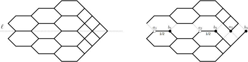
Figure 1. Left. A plane bipartite symmetric graph $G$. Right. The graphs $G^{+}$ (on top) and $G^{-}$ (on the bottom) corresponding to $G$.

Let $G$ be a weighted symmetric graph with symmetry axis $\ell$, which we consider to be horizontal. Let $a_{1},b_{1},a_{2},b_{2},\dotsc$ be the vertices lying on $\ell$, as they occur from left to right (if $G$ has an even number of vertices, this sequence ends with $b_{\operatorname{w}(G)}$, while if $G$ has an odd number of vertices, it ends with $a_{\operatorname{w}(G)+1}$).

The weight of a matching $\mu$ is defined to be the product of the weights of the edges contained in $\mu$. The matching generating function of a weighted graph $G$, denoted $\operatorname{M}(G)$, is the sum of the weights of all matchings of $G$. The matching generating function is clearly multiplicative with respect to disjoint unions of graphs. We will henceforth assume that all graphs under consideration are connected.

Let $G$ be a weighted symmetric graph that is also bipartite. For definiteness, choose the leftmost vertex on the symmetry axis $\ell$ to be white. We define two subgraphs $G^{+}$ and $G^{-}$ as follows.

Given a vertex $u$ of $G$ on the symmetry axis, we call the operation of deleting all edges incident to $u$ above $\ell$ cutting above $u$; similarly, we call deleting all edges incident to $u$ below $\ell$ cutting below $u$. Perform cutting operations above all white $a_{i}$’s and black $b_{i}$’s and below all black $a_{i}$’s and white $b_{i}$’s. Note that this procedure yields cuts of the same kind at the endpoints of each edge lying on $\ell$ (see the proof of Theorem 2.1 for a justification). Reduce the weight of each such edge by half; leave all other weights unchanged.

As shown in the proof of Theorem 2.1(a), the graph produced by the above procedure is disconnected into one part lying above and one lying below $\ell$. Denote the portion above $\ell$ by $G^{+}$, and the one below $\ell$ by $G^{-}$; see Figure 1 for an illustration of this procedure (the edges whose weight has been reduced by half are marked by 1/2).

Part (a) of the following result is a slight strengthening of the original factorization theorem of [5, Theorem 1.2] (namely, we show that the assumption made there that the graph is separated by its symmetry axis can be dropped). The new version is contained in part (b).

Theorem 2.1.

Let $G$ be a plane bipartite weighted symmetric graph.

$($a$)$. If $G$ has an even number of vertices, then

$$\operatorname{M}(G)=2^{\operatorname{w}(G)}\operatorname{M}(G^{+})\operatorname{M}(G^{-}).$$ (2.1)

$($b$)$. Suppose $G$ has an odd number of vertices and $v$ is a vertex on the unbounded face of $G$ lying off the symmetry axis. Then

$$\operatorname{M}_{v}(G)=\begin{cases}2^{\operatorname{w}(G)}\operatorname{M}(G^{+})\operatorname{M}_{v^{\prime}}(G^{-}),&\text{\rm if $v$ is white,}\\ 2^{\operatorname{w}(G)}\operatorname{M}_{v}(G^{+})\operatorname{M}(G^{-}),&\text{\rm if $v$ is black,}\end{cases}$$ (2.2)

where $v^{\prime}$ is the mirror image of $v$.

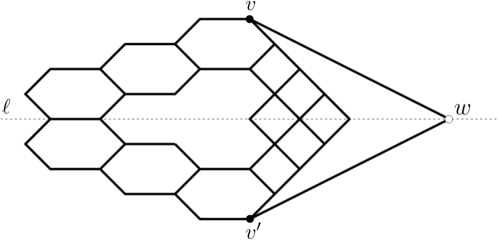
Figure 2. The graph $\overline{G}$ corresponding to the graph $G$ shown in Figure 1 with one vertex removed (since the graph in Figure 1 has the same number of white and black vertices, we have to delete from it a vertex on $\ell$ of the color opposite to the color of $v$ in order to obtain a graph meeting the hypotheses of part (b) of Theorem 2.1).

To prove (a), it suffices to show that our assumptions imply that the graph $G_{0}$ produced by the cutting procedure described before stating Theorem 2.1 above is disconnected into one part lying above and one lying below $\ell$. Namely, we need to show that there exists a Jordan arc $J$ in the plane connecting some point $A$ on $\ell$ to some point $B$ on $\ell$ — where $A$ is to the left of $a_{1}$, and $B$ is to the right of $b_{\operatorname{w}(G)}$ — so that the portion $H$ of $G_{0}$ which is above or on $\ell$ is above $J$, while the portion $K$ of $G_{0}$ which is below or on $\ell$ is below $J$.

To see this, note first that, as mentioned above, the cuts at the endpoints of each edge lying on $\ell$ are of the same kind — both above, or both below $\ell$; this is because we cut above white $a_{i}$’s and black $b_{i}$’s (and below black $a_{i}$’s and white $b_{i}$’s), and if an edge lies along $\ell$, its endpoints have on the one hand opposite color, and on the other opposite $a_{i}$- or $b_{i}$-type.

Secondly, note that $G_{0}$ cannot have any edge $\{u,v\}$ with $u$ above $\ell$ and $v$ below $\ell$. Indeed, if $u$ and $v$ are not mirror images with respect to $\ell$, the symmetry of $G$ implies that the mirror images $u^{\prime}$ and $v^{\prime}$ of $u$ and $v$ form another edge $\{u^{\prime},v^{\prime}\}$ of $G_{0}$; but then the edges $\{u,v\}$ and $\{u^{\prime},v^{\prime}\}$ would cross, which is a contradiction, since $G$ is a plane graph. On the other hand, if $u$ and $v$ are mirror images of each other, let $P$ be a path in $G$ connecting $u$ to $a_{1}$ (as $G$ is assumed to be connected, such a path exists). Then the mirror image $P^{\prime}$ of $P$ across $\ell$ is a path in $G$ connecting $v$ to $a_{1}$. Since $P$ and $P^{\prime}$ have the same length and $G$ is bipartite, it follows that $u$ and $v$ have the same color, so the edge $\{u,v\}$ has endpoints of the same color; this contradicts the fact that $G$ is bipartite.

By the second to last paragraph, we can connect $A$ to $B$ by a Jordan arc $J$ which does not cross any edge of $G_{0}$ incident to a vertex on $\ell$. By the previous paragraph, this arc $J$ does not cross any other edge of $G_{0}$ either. This proves our claim, and completes the proof of part (a).

To prove part (b), note first that unless the difference between the number of white and black vertices of $G$ is $\pm 1$, and in addition $v$ has the color of the majority of vertices, equation (2.2) holds trivially, as both sides equal zero. Therefore, without loss of generality we may assume that these conditions hold.

Next, define $\overline{G}$ to be the graph obtained from $G$ by including a new vertex $w$ on $\ell$ contained in the unbounded face of $G$, and the two new edges $\{w,v\}$ and $\{w,v^{\prime}\}$ (both weighted by 1), where $v^{\prime}$ is the mirror image of $v$ (see Figure 2). Then $\overline{G}$ is a plane, bipartite, weighted symmetric graph, to which the factorization theorem [5, Theorem 1.2] can be applied.

If $v$ is white, $w$ is black, and (since $w$ is also a $b_{i}$-type vertex) the cutting operation at $w$ prescribed by the factorization theorem occurs above $w$. Therefore, $\overline{G}^{+}$ is precisely $G^{+}$. Furthermore, in $\overline{G}^{-}$ vertex $w$ has degree one, and after removing the edge that is forced to match it, the resulting graph (which has the same matching generating function as $\overline{G}^{+}$, as the removed edge has weight 1) is precisely $G^{-}\setminus v^{\prime}$. Thus the factorization theorem applied to $\overline{G}$ yields

$$\operatorname{M}(\overline{G})=2^{\operatorname{w}(G)+1}\operatorname{M}(G^{+})\operatorname{M}(G^{-}\setminus v^{\prime})=2^{\operatorname{w}(G)+1}\operatorname{M}(G^{+})\operatorname{M}_{v^{\prime}}(G^{-}).$$ (2.3)

On the other hand, since in $\overline{G}$ the vertex $w$ can only be matched to $v$ or $v^{\prime}$, and since $G\setminus v$ and $G\setminus v^{\prime}$ are isomorphic, it follows that $\operatorname{M}(\overline{G})=2\operatorname{M}(G\setminus v)=2\operatorname{M}_{v}(G)$. Combined with (2.3), this proves (2.2) when $v$ is white. The case when $v$ is black follows by the same argument.

The second result in this section is more specific, but is general enough so that it has several interesting consequences, including solutions to two open problems posed by Lai (see Sections 4 and 5), closed formulas for the number of lozenge tilings of some new families of hexagonal regions with holes (see Section 5), and an extension of a result by Fulmek and Krattenthaler (see Section 6).

Draw the triangular lattice so that one family of lattice lines is horizontal, and let $H$ be a hexagonal region on this lattice, symmetric about a vertical symmetry axis $\ell$. Let $R_{0}$ be the region obtained from $H$ by removing an arbitrary collection ${\mathcal{C}}$ of unit triangles, so that ${\mathcal{C}}$ is symmetric about $\ell$ and contains no unit triangles touching the southern or southeastern edge of $H$. Define $R$ to be the region obtained from $R_{0}$ by translating all unit triangles in ${\mathcal{C}}$ one unit in the southeastern lattice direction. We call the region $R$ a nearly symmetric hexagon with holes. Therefore, while the outer, hexagonal boundary of the region $R$ is symmetric with respect to the original symmetry axis $\ell$, the holes in $R$ are symmetric about the line $\ell^{\prime}$, the translation of $\ell$ half a unit to the right.

Let $G$ be the planar dual graph of $R$. Even though $G$ is not symmetric about $\ell^{\prime}$, let us consider the graphs $G^{+}$ and $G^{-}$ obtained from it by rotating it 90 degrees counterclockwise and performing cutting operations around the vertices on $\ell^{\prime}$ as prescribed by the factorization theorem (assuming, in particular, that after the rotation the leftmost vertex on $\ell^{\prime}$ is white). In addition to these two graphs, consider also the graphs $\hat{G}^{+}$ and $\hat{G}^{-}$ obtained from $G$ by performing cutting operations around the vertices on $\ell^{\prime}$ as prescribed by the factorization theorem, but assuming this time that after the rotation the leftmost vertex on $\ell^{\prime}$ is black. Define $R^{+}$, $R^{-}$, $\hat{R}^{+}$ and $\hat{R}^{-}$ to be the lattice regions whose planar duals are the graphs $G^{+}$, $G^{-}$, $\hat{G}^{+}$ and $\hat{G}^{-}$, respectively.

We can now state our second result in this section.

Theorem 2.2.

Let $R$ be a nearly symmetric hexagon with holes, and assume that $R$ admits at least one lozenge tiling. Then the number of lozenge tilings of $R$ is given by

$$\operatorname{M}(R)=2^{\operatorname{w}_{\ell^{\prime}}(R)-1}\left(\operatorname{M}(R^{+})\operatorname{M}(R^{-})+\operatorname{M}(\hat{R}^{+})\operatorname{M}(\hat{R}^{-})\right),$$ (2.4)

where $\operatorname{w}_{\ell^{\prime}}(R)$ is half the number of unit triangles in $R$ crossed by $\ell^{\prime}$.

Remark $1$. Formula (2.3) has the following amusing interpretation. The nearly symmetric hexagon with holes $R$ is not quite symmetric about $\ell^{\prime}$, but its holes are, so we might expect that if we form the expression on the right hand side of the factorization theorem (see equation (2.1)), the resulting number will be a reasonable estimate for $\operatorname{M}(R)$. But note: there are two ways to form this expression, depending on whether we consider the vertex $a_{1}$ in the factorization theorem to be white or black! (For symmetric graphs, these two ways are equivalent, because they result in isomorphic pairs of graphs, due to the symmetry.) Form then both these expressions, and average them, to get an even more reasonable estimate. Then Theorem 2.2 states that this latter “estimate” is actually the exact value of $\operatorname{M}(R)$.

This phenomenon turns out to be very sensitive to changing the shape of the outer boundary of the region. For it to hold, it seems essential that the outer boundary is a symmetric hexagon, with symmetry axis half a unit away from the symmetry axis of the holes.

Our proof of the above theorem employs Kuo’s graphical condensation [24]. Let $G$ be a plane bipartite graph, $V_{1}$ and $V_{2}$ the vertex sets of the graph consisting of the two color classes, and $E$ the edge set of the graph. For any subset $W\subset V_{1}\cup V_{2}$ of vertices of $G$, let $G\setminus W$ be the subgraph obtained from $G$ by deleting all vertices in $W$ and all their incident edges.

Theorem 2.3 (Theorem 5.2 in [24]).

Let $G=(V_{1},V_{2},E)$ be a weighted plane bipartite graph in which $|V_{1}|=|V_{2}|$. Let vertices $a,b,c,$ and $d$ appear in a cyclic order on the same face of $G$. If $a,b\in V_{1}$ and $c,d\in V_{2}$, then

$$\operatorname{M}(G-\{a,d\})\operatorname{M}(G-\{b,c\})=\operatorname{M}(G)\operatorname{M}(G-\{a,b,c,d\})+\operatorname{M}(G-\{a,c\})\operatorname{M}(G-\{b,d\}).$$

[Proof of Theorem 2.2] The pictures are slightly different, depending on the parity of the length of the top and the bottom side of the region $R$ (there are $2\times 2=4$ cases). Here, we only present the pictures for one case (when the length of the top side of $R$ is odd and the length of the bottom side of $R$ is even); the other cases follow similarly.

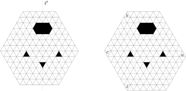
Figure 3. A nearly symmetric hexagon with holes, denoted by $R$ (left), and the extended region $\hat{R}$ (right). The positions of four unit triangles $a,b,c,$ and $d$ are marked on $\hat{R}$.

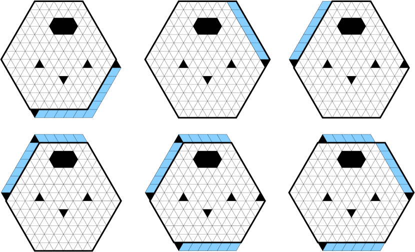
Figure 4. The six regions appearing in the recurrence obtained by applying Kuo condensation to the extended region $\hat{R}$, with the indicated choice of the unit triangles $a,b,c,$ and $d$.

We first add one layer of unit triangles on the bottom and bottom right side of $R$, as can be seen Figure 3, denote the resulting region by $\hat{R}$, and call it the extended region $\hat{R}$. We then choose four unit triangles $a,b,c,$ and $d$ along the boundary of $\hat{R}$ as shown in the right picture in Figure 3. The dual graph of $\hat{R}$ and the four vertices of the dual graph that correspond to unit triangles $a,b,c,$ and $d$ satisfy the conditions in Kuo’s graphical condensation. If one applies Kuo’s graphical condensation in this way on the dual graph of $\hat{R}$ and then take the dual again, one gets the following recurrence relation (Figure 4 shows the six regions appearing in the recurrence):

$$\operatorname{M}(\hat{R}-\{a,d\})\operatorname{M}(\hat{R}-\{b,c\})=\operatorname{M}(\hat{R})\operatorname{M}(\hat{R}-\{a,b,c,d\})+\operatorname{M}(\hat{R}-\{a,c\})\operatorname{M}(\hat{R}-\{b,d\}).$$

After removing some forced lozenges, one can observe that $\hat{R}-\{a,d\}=R$, $\hat{R}-\{b,c\}$ is a symmetric region (see the bottom left picture in Figure 4). Furthermore, each of two regions $\hat{R}-\{a,b,c,d\}$ and $\hat{R}-\{a,c\}$ can be viewed as being obtained from a symmetric region with a unit dent on the boundary, after removing the lozenges forced by this dent (see the bottom center picture and top right picture, respectively in Figure 4). In fact, the remaining two regions, $\hat{R}$ and $\hat{R}\setminus\{b,d\}$, can also be seen as symmetric regions with defects on their boundary, but we need to enlarge the regions to see that. In the case of $\hat{R}$, we add one layer of unit triangles on the top right side of $\hat{R}$, and remove the bottom-most of these (see the top center picture in Figure 4). The region $\hat{R}\setminus\{b,d\}$ can be handled similarly, but we first remove from it the forced lozenges along the top and bottom sides (see the bottom right picture in Figure 4).

We now identify each of these five regions with the corresponding symmetric region (resp., symmetric region with a unit boundary dent) that we described above. Under this identification, we can apply Theorem 2.1(a) to $\hat{R}-\{b,c\}$ and Theorem 2.1(b) to the four regions $\hat{R}$, $\hat{R}-\{a,b,c,d\}$, $\hat{R}-\{a,c\}$, and $\hat{R}-\{b,d\}$. If we apply Theorem 2.1, then the powers of two in the factorizations of $\operatorname{M}(\hat{R}-\{b,c\})$, $\operatorname{M}(\hat{R})$, and $\operatorname{M}(\hat{R}-\{a,c\})$ are $2^{w_{l^{\prime}}(R)}$, while those in the factorizations of $\operatorname{M}(\hat{R}-\{a,b,c,d\})$ and $\operatorname{M}(\hat{R}-\{b,d\})$ are $2^{w_{l^{\prime}}(R)-1}$. Figure 5 shows how the five regions are split via Theorem 2.1; note that the first branch of Theorem 2.1(b) is applied when the unit boundary dent (which corresponds to $v$) has the same orientation as the top unit triangle along the symmetry axis (which corresponds to $a_{1}$), and the second branch when the orientations are opposite. One readily sees that the resulting “half”-subregions — we call them parts — have the following properties:

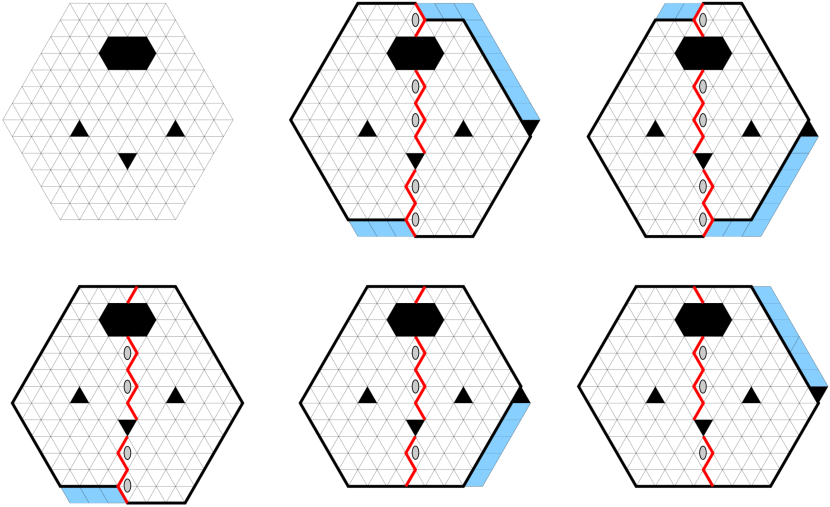
Figure 5. Applying Theorem 2.1 (a) and (b) to the five regions.

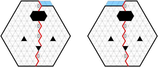
Figure 6. The two different ways of decomposing $R$ into parts, using zigzag lines along $\ell^{\prime}$ as prescribed in the factorization theorem.

• The left part of $\hat{R}-\{b,c\}$ is the same (up to forced lozenges) as the left half of $\hat{R}-\{a,b,c,d\}$, and the right part of $\hat{R}-\{b,c\}$ is the same (up to some forced lozenges) as the right part of $\hat{R}$.

• The left part of $\hat{R}-\{b,c\}$ is the same as the right part of $\hat{R}-\{b,d\}$, and the right part of $\hat{R}-\{b,c\}$ is the same (up to forced lozenges) as the left part of $\hat{R}-\{a,c\}$.

• The remaining two parts of $\hat{R}$ and $\hat{R}-\{a,b,c,d\}$ (the ones which are not the same as any of the parts of $\hat{R}-\{b,c\}$) can be identified with the two parts of $R$ obtained when we split $R$ using one of the two zigzag lines along $\ell^{\prime}$, as prescribed by the factorization theorem (compare the two picture at the center in Figure 5 and the left picture in Figure 6).

• The remaining two parts of $\hat{R}-\{a,c\}$ and $\hat{R}-\{b,d\}$ (the ones which cannot be identified with any part of $\hat{R}-\{b,c\}$), can be identified (up to forced lozenges) with the two parts of $R$ when we split $R$ using the other zigzag line along $\ell^{\prime}$, as prescribed by the factorization theorem (compare the two picture on the right in Figure 5 and the right picture in Figure 6).

Combining the above observations and the fact that $\operatorname{M}(\hat{R}-\{a,d\})=\operatorname{M}(R)$, we get the desired identity.

3. Solution of Four Open Problems of Propp

Figure 7. The $(a,b)$-benzel for $a=7$, $b=8$.

In this section, we solve four open problems posed by Propp on the enumeration of trimer coverings of regions called benzels. To state the problems, we first define the benzel regions. For any positive integers $a$ and $b$ such that $2\leq a\leq 2b$ and $2\leq b\leq 2a$, we defined the $(a,b)$-benzel as follows. Consider a hexagonal grid on the plane consisting of regular hexagons of side length $1$, each having two horizontal sides (see Figure 7; this can be thought as a tessellation of the plane by unit hexagons). We call these unit hexagons cells. Regard the plane as the complex plane so that the origin is the left vertex of one of the cells. Let $H$ be the hexagon whose vertices are $\omega^{j}(a\omega+b)$ and $-\omega^{j}(a+b\omega)$ for $j\in\{0,1,2\}$, where $\omega=e^{2\pi i/3}$. Then, the $(a,b)$-benzel is defined to be the union of all the cells that are contained in the hexagon $H$; Figure 7 shows the $(7,8)$-benzel.

Figure 8. Left stone, right stone, vertical bone, rising bone, and falling bone (left to right).

Propp considered tilings of the benzel using two types of tiles, called stones and bones. A stone is the union of three cells that are pairwise adjacent. A bone is the union of three contiguous cells whose centers are collinear. Taking orientation into account, there are five different types of tiles: the left stone, the right stone, the vertical bone, the rising bone, and the falling bone (see Figure 8). Given a benzel, a trimer cover of the region is a collection of stones and bones that covers the region without gaps or overlaps. By considering various restrictions on what tiles are allowed to be used, and the fact that the detailed shape of the $(a,b)$-benzel depends on the residues of $a$ and $b$ modulo 3, Propp was led to twenty open problems, stated in [31]. Out of these, the first eighteen conjecture either explicit formulas or explicit recurrences for the number of trimer covers, while the last two concern combinatorial, resp. number theoretic properties of these numbers.

One example is: “How many trimer covers does the $(a,b)$-benzel have, in which all the three types of bones, but not both types of stones are allowed?” (Problem 3 in [31]). See [16][17][22] for recent progress on some of these problems. The open problems that we solve in this section are about the enumeration of trimer covers of benzels that can use both kinds of stones, the rising bone and the falling bone (in other words, the only restriction is that they cannot use any vertical bone). In this paper, we call such tilings vertical-bone-free tilings. Based on numerical data, Propp conjectured that the number of such trimer covers of the $(3n,3n)$-benzel (Problem 8), the $(3n+1,3n+1)$-benzel (Problem 9), the $(3n+1,3n+2)$-benzel (Problem 10), and the $(3n-1,3n)$-benzel (Problem 11) satisfy explicit recurrence relations. Proving such statements is in principle very hard, as, in contrast to the situation of dimer coverings, there are not many enumeration techniques available for trimer covers.

Recently, Defant et al.[16] found a very useful bijection, which they call compression, allowing one to convert trimer enumeration problems into dimer enumeration problems (see Section 3 in [16] for more details about this bijection). This opens up the possibility of proving some of Propp’s conjectures using dimer enumeration techniques. We now introduce four families of regions whose domino tiling enumeration (equivalently, perfect matching enumeration of their planar dual graphs) are equivalent, thanks to the results in [16], to Problems 8–11 from Propp’s list.

Recall that for a positive integer $n$, the Aztec diamond of order $n$, denoted $AD_{n}$, is the region consisting of all the unit squares on $\mathbb{Z}^{2}$ whose centers $(x,y)$ satisfy the inequality $|x|+|y|\leq n$ (Figure 9 illustrates the Aztec diamond of order $7$).

Figure 9. Aztec diamond of order $7$, denoted by $AD(7)$.

Figure 10. $TAD_{7}$ (top left), $TAD_{8}$ (top right), $TAD^{\prime}_{7}$ (bottom left), and $TAD^{\prime}_{8}$ (bottom right).

The four families of regions mentioned above, which we denote by $TAD_{2n-1}$, $TAD_{2n}$, $TAD^{\prime}_{2n-1}$, $TAD^{\prime}_{2n}$, are simple truncations of the Aztec diamonds, obtained as follows.

To obtain the region $TAD_{2n-1}$, start with the Aztec diamond $AD_{2n-1}$, and consider the lattice point $P$ on its southwestern boundary which lies on its southwest-to-northeast going symmetry axis. The portion of $AD_{2n-1}$ contained in the “northeast quadrant” centered at $P$ is the region $TAD_{2n-1}$ (the top left picture in Figure 10 shows $TAD_{7}$). The region $TAD_{2n}$ is defined in the same way, starting with $AD_{2n}$ ($TAD_{8}$ is shown on the top right of Figure 10); the reason we consider separately the cases of even and odd indices is because the details of their boundaries are slightly different, and this will be reflected in their tiling enumeration formulas.

The region $TAD_{2n-1}^{\prime}$ is defined almost exactly like $TAD_{2n-1}$, with the one difference that the boundary lattice point from which the above-described truncation is performed is not the point $P$ that lies on the southwest-to-northeast going symmetry axis, but is chosen instead to be the boundary point $P^{\prime}$ which is one unit step north of $P$ (the bottom left picture in Figure 10 illustrates $TAD_{7}^{\prime}$). Similarly, the only difference between $TAD^{\prime}_{2n}$ and $TAD_{2n}$ is that for the former the truncation of $AD_{2n}$ is not performed from $P$, but from the lattice point which is one unit step west of $P$; the bottom right picture in Figure 10 illustrates $TAD^{\prime}_{8}$.

As mentioned above, using their compression bijection, Defant et al. restated Problems 8–11 on Propp’s list in terms of perfect matching problems (see Conjectures 5.1–5.3 and Question 5.4 in [16]). Using the natural bijection between domino tilings of regions and perfect matchings of their planar dual graphs, their results can be rephrased as follows:

• The number of vertical-bone-free tilings of the $(3n,3n)$-benzel is $\operatorname{M}(TAD_{2n-1})$.

• The number of vertical-bone-free tilings of the $(3n+1,3n+1)$-benzel is $\operatorname{M}(TAD_{2n})$.

• The number of vertical-bone-free tilings of the $(3n-1,3n)$-benzel is $\operatorname{M}(TAD^{\prime}_{2n-1})$.

• The number of vertical-bone-free tilings of the $(3n+1,3n+2)$-benzel is $\operatorname{M}(TAD^{\prime}_{2n})$.

Thus, to prove Propp’s original conjectures, it suffices to enumerate the domino tilings of $TAD_{2n-1}$, $TAD_{2n}$, $TAD^{\prime}_{2n-1}$, and $TAD^{\prime}_{2n}$. The main result of this section, Theorem 3.1 below, provides explicit, simple product formulas for the number of domino tilings of these regions.

Theorem 3.1.

For positive integers $n$, the numbers of domino tilings of the regions $TAD_{2n-1}$, $TAD_{2n}$, $TAD^{\prime}_{2n-1}$, and $TAD^{\prime}_{2n}$ are given by the following product formulas:

$$\operatorname{M}(TAD_{2n-1})=2^{n^{2}}\cdot\frac{(2n-1)!!}{n!}\cdot\prod_{i=1}^{2n-1}\frac{(2i)!}{(n+i)!},$$ (3.1)

$$\operatorname{M}(TAD_{2n})=2^{n(n+1)}\cdot\prod_{i=0}^{n-1}\frac{(4i+2)!(4i+3)!}{(n+2i+1)!(n+2i+2)!},$$ (3.2)

$$\operatorname{M}(TAD^{\prime}_{2n-1})=2^{n^{2}-1}\cdot\prod_{i=0}^{n-1}\frac{(4i+2)!}{(n+2i+1)!}\cdot\prod_{i=0}^{n-2}\frac{(4i+3)!}{(n+2i+1)!}.$$ (3.3)

and

$$\operatorname{M}(TAD^{\prime}_{2n})=2^{n(n+1)}\cdot\frac{(2n+1)!!}{(n+1)!}\cdot\prod_{i=0}^{n-1}\frac{(4i+2)!(4i+4)!}{(n+2i+1)!(n+2i+3)!}.$$ (3.4)

Corollary 3.2.

For any positive integer $n$,

• The number of vertical-bone-free tilings of $(3n,3n)$-benzel is given by (3.1).

• The number of vertical-bone-free tilings of $(3n+1,3n+1)$-benzel is given by (3.2).

• The number of vertical-bone-free tilings of $(3n-1,3n)$-benzel is given by (3.3).

• The number of vertical-bone-free tilings of $(3n+1,3n+2)$-benzel is given by (3.4).

Figure 11. Top half of $AD_{3}$, $ZH_{7}$, and $ZH_{8}$ (from left to right).

Figure 12. The Aztec triangles $AT_{1}(4)$, $AT_{2}(4)$, $AT_{3}(4)$, and $AT_{4}(5)$ (from left to right).

The proof of the above theorem is based on Theorem 2.1(a) (for (3.1) and (3.2)), Theorem 2.1(b) (for (3.3) and (3.4)), and some enumeration results of Corteel et al. presented in [15].

We need to introduce four families of regions, which are special cases of more general regions whose number of domino tilings were studied in [15]. To describe them, note that the square of side length $2n$ can be split into two congruent subregions using a zigzag line of step 2 along its diagonal, which has positive slope, and that there are two choices for the zigzag line. Depending on this choice, the subregion on the top left either has width $2n-1$ or $2n$ (see Figure 11). We call the former $ZH_{2n-1}$ and the latter $ZH_{2n}$. If we glue above $ZH_{2n-1}$ the top half of $AD_{n-1}$ in a right-justified manner, the resulting region is called the Aztec triangle of order $n$; we denote it by $AT_{1}(n)$ (the leftmost picture in Figure 12 is $AT_{1}(4)$).

The second family of regions (also illustrated in Figure 12, as are the regions in the last two families) is constructed in almost exactly the same way: the only difference is that the top half of $AD_{n-1}$ is glued on above $ZH_{2n-1}$ in a left-justified fashion; we denote the resulting region by $AT_{2}(n)$.

To obtain the regions $AT_{3}(n)$ in the third family, we glue above $ZH_{2n}$ the top half of $AD_{n}$ so that the top side of the former and the bottom side of the latter match up (this can be done since both sides have length $2n$). Finally, the region $AT_{4}(n+1)$ of the fourth family is constructed almost exactly like the previous region $AT_{3}(n)$, with the one difference that before matching up the sides of the two constituent parts, we insert between them a horizontal strip consisting of $2n$ unit squares (these two regions are also shown in Figure 12). We will find it convenient to have the indexing of the regions in the last family shifted by one unit, as in the above definition. But due to this, we need to define $AT_{4}(1)$ separately: we set $AT_{4}(1)$ to be the empty region, which has one domino tiling (the empty set of dominos).

These four families of regions turn out to be special cases of regions considered by Corteel et al. in [15]. In that paper, the authors consider a family of regions parametrized by positive integers $l$ and $k$. The regions $AT_{1}(n)$ represents the special case $l=2n$ and $k=n$. Furthermore, $AT_{2}(n)$ is the special case $l=2n+1$ and $k=n-1$, $AT_{3}(n)$ the special case $l=2n+1$ and $k=n$, and $AT_{4}(n)$ is obtained by setting $l=2n$ and $k=n-1$.

By specializing the values of $l$ and $k$ in Theorem 1.2 of [15] as indicated in the previous paragraph, we obtain the following enumeration results for the number of domino tilings of these four families of regions.

Lemma 3.3.

For positive integers $n$, the number of domino tilings of the regions $AT_{1}(n)$, $AT_{2}(n)$, $AT_{3}(n)$, and $AT_{4}(n)$ are given by the following formulas.

$$\operatorname{M}(AT_{1}(n))=\operatorname{M}(AT_{2}(n))=2^{n(n-1)/2}\cdot\prod_{i=0}^{n-1}\frac{(4i+2)!}{(n+2i+1)!},$$ (3.5)

$$\operatorname{M}(AT_{3}(n))=2^{n(n+1)/2}\cdot\prod_{i=0}^{n-1}\frac{(4i+3)!}{(n+2i+2)!},$$ (3.6)

and

$$\operatorname{M}(AT_{4}(n))=2^{n(n-1)/2}\cdot\frac{(2n-1)!!}{n!}\cdot\prod_{i=0}^{n-1}\frac{(4i)!}{(n+2i)!}.$$ (3.7)

The equality $\operatorname{M}(AT_{1}(n))=\operatorname{M}(AT_{2}(n))$ was proved by Corteel et al. in [15] by showing that the two numbers are given by the same formula. Recently, a bijective proof was given in [3] by the first two authors of the current paper.

[Proof of Theorem 3.1] The first two equalities 3.1 and 3.2 turn out to be direct consequences of the factorization theorem for perfect matchings (Theorem 2.1(a)) and the specializations of [15, Theorem 1.2] stated in Lemma 3.3. Indeed, note that the regions $TAD_{2n-1}$ and $TAD_{2n}$ are symmetric about their diagonals (with positive slope). If we apply the factorization theorem along these symmetry axes, we get, after removing some forced dominos (see Figure 13)

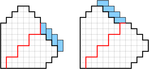
Figure 13. Left. Factorization of $TAD_{7}$ into $AT_{1}(4)$ and $AT_{4}(4)$. Right. Factorization of $TAD_{8}$ into $AT_{2}(4)$ and $AT_{3}(4)$.

$$\operatorname{M}(TAD_{2n-1})=2^{n}\cdot\operatorname{M}(AT_{1}(n))\cdot\operatorname{M}(AT_{4}(n)),$$ (3.8)

and

$$\operatorname{M}(TAD_{2n})=2^{n}\cdot\operatorname{M}(AT_{2}(n))\cdot\operatorname{M}(AT_{3}(n)).$$ (3.9)

The situation is different for the regions $TAD^{\prime}_{2n-1}$ and $TAD^{\prime}_{2n}$, as they are not symmetric. To apply Theorem 2.1(b), we first “symmetrize” these regions about their diagonals; denote by $\overline{TAD^{\prime}}_{2n-1}$ and $\overline{TAD^{\prime}}_{2n}$, respectively, the resulting symmetric regions (in Figure 14, these are the regions enclosed by the outermost contours). These new regions have no domino tilings, as they have an odd number of vertices. Let $v$ be the rightmost unit square in the top row of these regions ($v$ is indicated in Figure 14 by a black unit square). Since after removing the forced dominos from $\overline{TAD^{\prime}}_{2n-1}\setminus v$ one obtains the region $TAD^{\prime}_{2n-1}$, these two regions have the same number of tilings. The same is true for the regions $\overline{TAD^{\prime}}_{2n}\setminus v$ and $TAD^{\prime}_{2n}$. Note that the dual graphs of $\overline{TAD^{\prime}}_{2n-1}\setminus v$ and $\overline{TAD^{\prime}}_{2n}\setminus v$ are symmetric graphs with a boundary defect, so we can apply Theorem 2.1(b) to them. Applying it we get (after removing the forced dominos; see Figure 14)

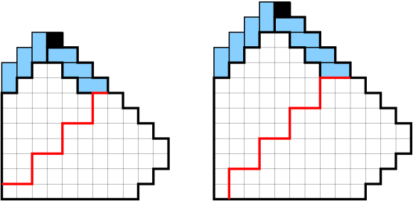
Figure 14. Factorization of $\overline{TAD^{\prime}}_{7}\setminus v$ into $AT_{2}(4)$ and $AT_{3}(3)$ (left) and that of $\overline{TAD^{\prime}}_{8}\setminus v$ into $AT_{1}(4)$ and $AT_{4}(5)$ (right). Black unit squares denote $v$ in both pictures.

$$\operatorname{M}(TAD^{\prime}_{2n-1})=\operatorname{M}(\overline{TAD^{\prime}}_{2n-1}\setminus v)=2^{n-1}\cdot\operatorname{M}(AT_{2}(n))\cdot\operatorname{M}(AT_{3}(n-1)),$$ (3.10)

and

$$\operatorname{M}(TAD^{\prime}_{2n})=\operatorname{M}(\overline{TAD^{\prime}}_{2n}\setminus v)=2^{n}\cdot\operatorname{M}(AT_{1}(n))\cdot\operatorname{M}(AT_{4}(n+1)).$$ (3.11)

It is straightforward to check that one gets expressions (3.1)–(3.4) by combining equations (3.5)–(3.7) and (3.8)–(3.11). This completes the proof.

Remark $2$. The original conjectures of Propp did not state explicit formulas for the number of vertical-bone-free tilings of benzels. Instead, the conjectures stated that those numbers satisfy certain recurrence relations. More precisely, via the compression bijection of [16], Propp’s conjectures (open Problems 8–11 in [31]) are equivalent to the following equalities ((3.12) and (3.15) were given in [31] and the other two in [16]):

$$\frac{\operatorname{M}(TAD_{2n-1})\operatorname{M}(TAD_{2n+3})}{\operatorname{M}(TAD_{2n+1})^{2}}=\frac{256(2n+3)^{2}(4n+1)(4n+3)^{2}(4n+5)}{27(3n+1)(3n+2)^{2}(3n+4)^{2}(3n+5)}$$ (3.12)

for all $n\geq 1$,

$$\frac{\operatorname{M}(TAD_{2n})}{\operatorname{M}(TAD_{2n-2})}=\frac{2^{2n}(4n-1)!(4n-2)!n!}{(3n)!(3n-1)!(3n-2)!}$$ (3.13)

for all $n\geq 2$,

$$\frac{\operatorname{M}(TAD^{\prime}_{2n-1})}{\operatorname{M}(TAD^{\prime}_{2n-3})}=\frac{2^{2n-3}(4n-2)!(4n-4)!(n-1)!!(n-3)!!}{(3n-1)!!(3n-2)!(3n-3)!(3n-5)!!}$$ (3.14)

for all $n\geq 2$, and

$$\frac{\operatorname{M}(TAD^{\prime}_{2n})\operatorname{M}(TAD^{\prime}_{2n+6})}{\operatorname{M}(TAD^{\prime}_{2n+2})\operatorname{M}(TAD^{\prime}_{2n+4})}$$ (3.15)

$$= \frac{65536(2n+3)(2n+5)^{2}(2n+7)(4n+3)(4n+5)^{2}(4n+7)^{2}(4n+9)^{2}(4n+11)}{729(3n+2)(3n+4)^{2}(3n+5)^{2}(3n+7)^{2}(3n+8)^{2}(3n+10)}$$

for all $n\geq 1$. It is straightforward to check that formulas (3.1)-(3.4) satisfy the above equalities (3.12)-(3.15); thus Corollary 3.2 indeed solves the four open problems of Propp.

Note also that deducing the simple product formulas (3.1)–(3.4) directly from the above recurrences would not be an easy task.

4. Nearly symmetric hexagons with collinear holes

In this section we solve an open problem posed by Lai, by providing an explicit product formula for the number of lozenge tilings of a certain family of hexagonal regions with holes on the triangular lattice (the regions $H^{\prime}_{\mathbf{l}}(a,b,k)$; see subsection 4.1 and Theorems 4.2(a) and 4.3(a)). This family is closely related to one of three families of symmetric hexagonal regions with collinear triangular holes (the regions $H_{\mathbf{l}}(a,b,k)$, also described in subsection 4.1) whose number of lozenge tilings was determined in [6] by the second author of the current paper: it is obtained from the latter by translating all the holes one unit in the southeast lattice direction. In addition to solving Lai’s open problem, we also provide explicit product formulas for two more families of regions, obtained from the two remaining families from [6] by the same procedure; see Theorems 4.2(b)(c) and 4.3(b)(c).

4.1. Six families of hexagonal regions with holes

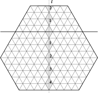
Figure 15. The labeling of the slots along a vertical line, starting from a reference horizontal lattice line; slots that are only partially contained in $H$ are also labeled.

We now recall the definitions of the three families of regions $H_{\mathbf{l}}(a,b,k)$, $H_{{\mathbf{l}},{\mathbf{q}}}(a,b,k)$ and $\bar{H}_{{\mathbf{l}},{\mathbf{q}}}(a,b,k)$ introduced in [6]; the other three families, $H^{\prime}_{\mathbf{l}}(a,b,k)$, $H^{\prime}_{{\mathbf{l}},{\mathbf{q}}}(a,b,k)$ and $\bar{H}^{\prime}_{{\mathbf{l}},{\mathbf{q}}}(a,b,k)$ are defined by a simple variation of these.

Draw the triangular lattice so that one of the families of lattice lines is horizontal, and let $H$ be a hexagon on this lattice. Let $\ell$ be a vertical line containing lattice points and crossing the interior of $H$. A slot is the union of two unit triangles crossed by $\ell$ which share an edge. Essential in the definition of our regions is the concept of labeling the slots contained in $H$, starting from a reference horizontal lattice line $L$. This is very simple: label the slots on both sides of $L$ successively by $1,2,3,\dotsc$ (the two closest ones by 1, the next two by 2, and so on), including also any slots that are only partially contained in $H$; this is illustrated in Figure 15.

Figure 16. Left. The symmetric hexagon with holes $H_{\mathbf{l}}(a,b,k)$ for $a=5$, $b=6$, $k=6$, and ${\mathbf{l}}=(1,2,5,7,8,9)$. Right. The corresponding nearly symmetric hexagon with holes $H^{\prime}_{\mathbf{l}}(a,b,k)$ for $a=5$, $b=6$, $k=6$, and ${\mathbf{l}}=(1,2,5,7,8,9)$.

Given non-negative integers $a$, $b$ and $k$, denote by $H(a,b,k)$ the hexagonal region on the triangular lattice whose side-lengths are $a$, $b+k$, $b$, $a+k$, $b$, $b+k$, clockwise from top. Thus $H(a,b,k)$ has $k$ more up-pointing unit triangles than down-pointing unit triangles. Our regions will be obtained from $H(a,b,k)$ by making some holes in it, so that the union of the holes has $k$ more up- than down-pointing triangles; this way, the resulting regions will have the same number of unit triangles of the two kinds, a necessary condition for the existence of lozenge tilings.

Let $\ell$ be the vertical symmetry axis of $H(a,b,k)$, and label the slots along $\ell$ choosing the reference line $L$ to be the base of $H(a,b,k)$ (see the picture on the left in Figure 16 for an example). Choose an arbitrary subset of the labeled slots along $\ell$ (avoiding the possible partial slot at the top), and for each chosen slot remove the up-pointing lattice triangle of side-length two containing that slot. If the resulting region has forced lozenges, remove them. Let ${\mathbf{l}}$ be the list of the labels of slots not covered by removed triangles in the resulting region. Then we denote the resulting region by $H_{\mathbf{l}}(a,b,k)$; an example is shown on the left in Figure 16.

The regions $H^{\prime}_{\mathbf{l}}(a,b,k)$ featured in Lai’s open problem are defined very similarly. Indeed, the only difference is that instead of the symmetry axis $\ell$, we consider its translation $\ell^{\prime}$ half a unit to the right, and we label the slots along $\ell^{\prime}$, with the reference line still being the base of $H(a,b,k)$. Letting ${\mathbf{l}}$ be the list of slot labels not covered by the removed triangles, the resulting region is defined to be $H^{\prime}_{\mathbf{l}}(a,b,k)$ (see the picture on the right in Figure 16 for an example).

The main new ingredient in the last two pairs of families of regions is that their definition also involves making one triangular hole of odd side-length. More precisely, let the reference line $L$ be a horizontal lattice line that meets the region $H(a,b,k)$, and consider again the symmetry axis $\ell$. Label the slots along $\ell$ with $L$ as the reference line, and remove an up-pointing triangle of odd size, symmetrically about $\ell$, whose base is along $L$. Then, as for the previous family, choose arbitrarily some labeled slots — now generating two subsets of labels, one for slots below $L$ and one for those above $L$. Then remove triangles of side two straddling the chosen slots, with an important difference: for the slots above $L$, choose them to be up-pointing, but for the slots below $L$ make them downpointing. Use the same convention about removing any forced lozenges. If in the resulting region the leftover labels below $L$ form the list ${\mathbf{l}}$, and those above $L$ the list ${\mathbf{q}}$, we define the resulting region to be $H_{{\mathbf{l}},{\mathbf{q}}}(a,b,k)$; an example is illustrated on the left in Figure 17. We define the region $H^{\prime}_{{\mathbf{l}},{\mathbf{q}}}(a,b,k)$ by applying exactly the same procedure, but with $\ell$ replaced by its half-unit translation to the right, $\ell^{\prime}$; see the picture on the right in Figure 17 for an example.

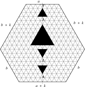
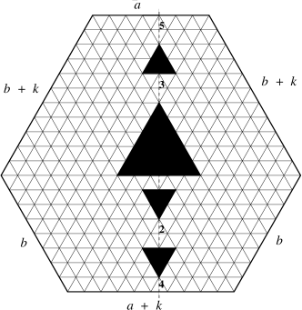
Figure 17. Left. The symmetric hexagon with holes $H_{{\mathbf{l}},{\mathbf{q}}}(a,b,k)$ for $a=7$, $b=8$, $k=3$, ${\mathbf{l}}=(2,4)$ and ${\mathbf{q}}=(3,5)$. Right. The corresponding nearly symmetric hexagon with holes $H^{\prime}_{{\mathbf{l}},{\mathbf{q}}}(a,b,k)$ for $a=7$, $b=8$, $k=3$, ${\mathbf{l}}=(2,4)$ and ${\mathbf{q}}=(3,5)$.

The last pair of families of regions is very similar to the previous one; the only difference is that the triangular hole of odd side-length is chosen to point downward. We denote the resulting regions by $\bar{H}_{{\mathbf{l}},{\mathbf{q}}}(a,b,k)$ and $\bar{H}^{\prime}_{{\mathbf{l}},{\mathbf{q}}}(a,b,k)$, respectively (these are illustrated in Figure 18).

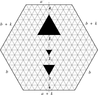
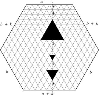
Figure 18. Left. The symmetric hexagon with holes $\bar{H}_{{\mathbf{l}},{\mathbf{q}}}(a,b,k)$ for $a=b=8$, $k=1$, ${\mathbf{l}}=(1,3,4)$ and ${\mathbf{q}}=(1,4)$. Right. The corresponding nearly symmetric hexagon with holes $\bar{H}^{\prime}_{{\mathbf{l}},{\mathbf{q}}}(a,b,k)$ for $a=b=8$, $k=1$, ${\mathbf{l}}=(1,3)$ and ${\mathbf{q}}=(1,4,5)$.

4.2. Two families of dented regions

We recall here the definitions of two more families of regions whose lozenge tilings were enumerated in [6]; they will be essential for solving Lai’s open problem. The detailed definitions are given in [6]; we rely here on Figures 20–22 to define our regions.

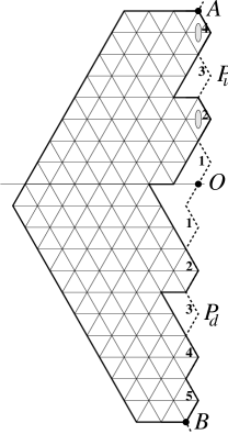
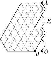
Figure 19. $R_{(2,4,5),(2,4)}(2)$

Figure 20. $R_{\emptyset,(2,4)}(4)$ (left) and $R_{(2,4,5),\emptyset}(2)$ (right).

Consider two semi-infinite vertical zigzag paths $P_{u}$ and $P_{d}$, meeting at the reference point $O$ as shown in Figure 20. Label the slots that fit in their folds (call these bumps) as shown in the figure. The tile positions corresponding to the bumps above $O$ are weighted by $1/2$ (this is indicated by shaded ellipses in the figures).

Given non-empty lists of strictly increasing positive integers ${\mathbf{l}}=(l_{1},\dotsc,l_{m})$ and ${\mathbf{q}}=(q_{1},\dotsc,q_{n})$ and a non-negative integer $x$, the region $R_{{\mathbf{l}},{\mathbf{q}}}(x)$ is defined as indicated in Figure 20. The lists ${\mathbf{l}}$ and ${\mathbf{q}}$ specify which bumps on the zigzag lines are kept. The kept bumps on $P_{u}$ are joined together by creating up-pointing dents, and those on $P_{d}$ by down-pointing dents; these two portions are then joined together via a horizontal ray left of $O$, as shown; $x$ is the length of the base. Note that this information, together with the fact that we want a region which can be tiled by lozenges, determines the rest of the boundary of $R_{{\mathbf{l}},{\mathbf{q}}}(x)$.

In case one of the lists ${\mathbf{l}}$ or ${\mathbf{q}}$ is empty, the definition is slightly different, as shown in Figure 20; note in particular that if ${\mathbf{l}}=\emptyset$, $x$ is not the length of the base, but one unit less than the distance from the left end of the base to the reference point $O$. Define $R_{\emptyset,\emptyset}(x)=\emptyset$ for all $x$.

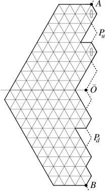
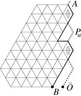
Figure 21. $\bar{R}_{(2,4,5),(2,4)}(3)$

Figure 22. $\bar{R}_{\emptyset,(2,4)}(5)$ (left) and $\bar{R}_{(2,4,5),\emptyset}(3)$ (right).

Our second family of regions, denoted $\bar{R}_{{\mathbf{l}},{\mathbf{q}}}(x)$, is defined almost identically (see Figures 22 and 22). The only difference is that, when connecting the upper and lower boundary portions determined by the selected bumps, instead of the horizontal ray starting from $O$, we use the one starting from the lattice point $\bar{O}$, one step southwest of $O$ (and, in case ${\mathbf{l}}$ is empty, when defining the bottom side of $\bar{R}_{\emptyset,{\mathbf{q}}}(x)$, we move left until we are $x$ units away from $\bar{O}$). Again, we define $\bar{R}_{\emptyset,\emptyset}(x)=\emptyset$ for all $x$.

4.3. Two families of polynomials and their connection to the dented regions

In this subsection, we introduce (1) monic polynomials $B_{m,n}(x)$ and $\bar{B}_{m,n}(x)$ for nonnegative integers $m$ and $n$, (2) constants $c_{\mathbf{l},\mathbf{q}}$ and $\bar{c}_{\mathbf{l},\mathbf{q}}$, and (3) polynomials $P_{\mathbf{l},\mathbf{q}}(x)$ and $\overline{P}_{\mathbf{l},\mathbf{q}}(x)$ for lists of strictly increasing positive integers ${\mathbf{l}}=(l_{1},\ldots,l_{n})$ and ${\mathbf{q}}=(q_{1},\ldots,q_{m})$. Before we define $B_{m,n}(x)$ and $\bar{B}_{m,n}(x)$, recall that for any positive integer (or half-integer) $a$ and nonnegative integer $k$, the Pochhammer symbol (sometimes called shifted factorial) $(a)_{k}$ is defined by setting $(a)_{0}\coloneqq 1$, and $(a)_{k}\coloneqq\prod_{i=1}^{k}(a+k-1)$ for positive integers $k$. In addition, for $a$ and $k$ like above, we will find it convenient to use the notation

$$\langle a,a+k\rangle \coloneqq\begin{cases}\displaystyle\prod_{i=0}^{k}(a+i)^{\text{min}(i+1,k+1-i)},&\text{if $k$ is nonnegative,}\\ 1,&\text{if $k$ is negative.}\end{cases}$$

$$=a(a+1)^{2}\cdots(a+k-1)^{2}(a+k)$$

$$=\prod_{i=0}^{\lfloor\frac{k}{2}\rfloor}(a+i)_{k+1-2i}.$$

With this notation, for nonnegative integers $m$ and $n$, $B_{m,n}(x)$ and $\bar{B}_{m,n}(x)$ are the monic polynomials given by

$$B_{m,n}(x)=\leavevmode\nobreak 2^{-mn-m(m-1)/2}(x+n+1)_{m}(x+n+2)_{m}\langle x+2,x+n\rangle\langle x+\frac{3}{2},x+\frac{2n+1}{2}\rangle$$

$$\cdot \prod_{i=1}^{n}\frac{(x+i)_{m}}{(x+i+1/2)_{m}}\prod_{i=1}^{m}(2x+n+i+2)_{n+i-1}$$

and

$$\bar{B}_{m,n}(x)=\leavevmode\nobreak 2^{-mn-n(n+1)/2}(x+m+1)_{n}\langle x+1,x+m\rangle\langle x+\frac{3}{2},x+\frac{2m-1}{2}\rangle$$

$$\cdot \prod_{i=1}^{m}\frac{(x+i)_{n}}{(x+i+1/2)_{n}}\prod_{i=1}^{n}(2x+m+i+1)_{m+i}.$$

For lists of strictly increasing positive integers ${\mathbf{l}}=(l_{1},\ldots,l_{n})$ and ${\mathbf{q}}=(q_{1},\ldots,q_{m})$, we define the constants $c_{\mathbf{l},\mathbf{q}}$ and $\bar{c}_{\mathbf{l},\mathbf{q}}$ by

$$c_{\mathbf{l},\mathbf{q}}=2^{\binom{n-m}{2}-m}\prod_{i=1}^{m}\frac{1}{(2l_{i})!}\prod_{i=1}^{n}\frac{1}{(2q_{i}-1)!}\frac{\prod_{1\leq i<j\leq m}(l_{j}-l_{i})\prod_{1\leq i<j\leq n}(q_{j}-q_{i})}{\prod_{i=1}^{m}\prod_{j=1}^{n}(l_{i}+q_{j})}$$

and

$$\bar{c}_{\mathbf{l},\mathbf{q}}=2^{\binom{n-m}{2}-m}\prod_{i=1}^{m}\frac{1}{(2l_{i}-1)!}\prod_{i=1}^{n}\frac{1}{(2q_{i})!}\frac{\prod_{1\leq i<j\leq m}(l_{j}-l_{i})\prod_{1\leq i<j\leq n}(q_{j}-q_{i})}{\prod_{i=1}^{m}\prod_{j=1}^{n}(l_{i}+q_{j})}.$$

We are now ready to define our polynomials $P_{\mathbf{l},\mathbf{q}}(x)$ and $\bar{P}_{\mathbf{l},\mathbf{q}}(x)$. For lists of strictly increasing positive integers ${\mathbf{l}}=(l_{1},\ldots,l_{n})$ and ${\mathbf{q}}=(q_{1},\ldots,q_{m})$, $P_{\mathbf{l},\mathbf{q}}(x)$ and $\bar{P}_{\mathbf{l},\mathbf{q}}(x)$ are given by

$$P_{\mathbf{l},\mathbf{q}}(x)=c_{\mathbf{l},\mathbf{q}}B_{m,n}(x+l_{m}-m) \prod_{i=1}^{m}\prod_{j=i}^{l_{i}-1}(x+l_{m}-j)(x+l_{m}-m+n+j+2)$$ (4.1)

$$\prod_{i=1}^{n}\prod_{j=i}^{q_{i}-1}(x+l_{m}-m+n-j+1)(x+l_{m}+j+1)$$

and

$$\bar{P}_{\mathbf{l},\mathbf{q}}(x)=\bar{c}_{\mathbf{l},\mathbf{q}}\bar{B}_{m,n}(x+l_{m}-m) \prod_{i=1}^{m}\prod_{j=i}^{l_{i}-1}(x+l_{m}-j)(x+l_{m}-m+n+j+1)$$ (4.2)

$$\prod_{i=1}^{n}\prod_{j=i}^{q_{i}-1}(x+l_{m}-m+n-j)(x+l_{m}+j+1).$$

In [6], the second author showed that the tilings generating functions of the two regions $R_{{\mathbf{l}},{\mathbf{q}}}(x)$ and $\bar{R}_{{\mathbf{l}},{\mathbf{q}}}(x)$ introduced in the subsection 4.2 are given by these polynomials $P_{\mathbf{l},\mathbf{q}}(x)$ and $\bar{P}_{\mathbf{l},\mathbf{q}}(x)$, respectively. More precisely,

$$\operatorname{M}(R_{{\mathbf{l}},{\mathbf{q}}}(x))=P_{\mathbf{l},\mathbf{q}}(x)$$ (4.3)

and

$$\operatorname{M}(\bar{R}_{{\mathbf{l}},{\mathbf{q}}}(x))=\bar{P}_{\mathbf{l},\mathbf{q}}(x).$$ (4.4)

4.4. Lozenge tilings of symmetric hexagons with holes along the symmetry axis.

For a region $R$ on the triangular grid, let $\operatorname{M}(R)$ be the number of lozenge tilings of the region. In [6], the second author determined the number of lozenge tilings of the regions $H_{\mathbf{l}}(a,b,k)$, $H_{\mathbf{l},\mathbf{q}}(a,b,k)$, and $\bar{H}_{\mathbf{l},\mathbf{q}}(a,b,k)$. The proof was based on the factorization theorem for matchings [5, Theorem 1.2] and equalities (4.3)–(4.4). The result (stated in a slightly different form) is the following.

Theorem 4.1 (Theorem 1.1 in [6]).

Let $H$ be one of the regions $H_{\mathbf{l}}(a,b,k)$, $H_{{\mathbf{l}},{\mathbf{q}}}(a,b,k)$ or $\bar{H}_{{\mathbf{l}},{\mathbf{q}}}(a,b,k)$. Then we have

$$\operatorname{M}(H)=2^{\operatorname{w}_{\ell}(H)}\operatorname{M}(H_{\ell}^{+})\operatorname{M}(H_{\ell}^{-}),$$ (4.5)

and all of the regions $H_{\ell}^{+}$ and $H_{\ell}^{-}$ are $R$- or $\bar{R}$-regions, as follows:

$($a$)$. For $k$ even, we have

$$[H_{\mathbf{l}}(a,b,k)^{+},H_{\mathbf{l}}(a,b,k)^{-}]=\begin{cases}[\bar{R}_{{\mathbf{l}}-1,\emptyset}(a/2),R_{\emptyset,{\mathbf{l}}}((a+k-2)/2)],&\text{$a$ even, $l_{1}=1$,}\\ [{R}_{{\mathbf{l}}-1,\emptyset}(a/2),R_{\emptyset,{\mathbf{l}}}((a+k-2)/2)],&\text{$a$ even, $l_{1}>1$,}\\ [\bar{R}_{{\mathbf{l}},\emptyset}((a-1)/2),R_{\emptyset,{\mathbf{l}}^{(m)}}((a+k-1)/2)],&\text{$a$ odd.}\end{cases}$$ (4.6)

$($b$)$. For $k$ odd, we have

$$[H_{{\mathbf{l}},{\mathbf{q}}}(a,b,k)^{+},H_{{\mathbf{l}},{\mathbf{q}}}(a,b,k)^{-}]=\begin{dcases}[{R}_{{\mathbf{q}},{\mathbf{l}}^{(m)}}(a/2),\bar{R}_{{\mathbf{l}},{\mathbf{q}}}((a+k-1)/2)],&\text{$a$ even,}\\ [{R}_{{\mathbf{q}},{\mathbf{l}}}((a-1)/2),\bar{R}_{{\mathbf{l}},{\mathbf{q}}^{(n)}}((a+k)/2)],&\text{$a$ odd,}\end{dcases}$$ (4.7)

and

$$[\bar{H}_{{\mathbf{l}},{\mathbf{q}}}(a,b,k)^{+},H_{{\mathbf{l}},{\mathbf{q}}}(a,b,k)^{-}]=\begin{dcases}[\bar{R}_{{\mathbf{q}},{\mathbf{l}}^{(m)}}(a/2),{R}_{{\mathbf{l}},{\mathbf{q}}}((a+k-1)/2)],&\text{$a$ even,}\\ [\bar{R}_{{\mathbf{q}},{\mathbf{l}}}((a-1)/2),{R}_{{\mathbf{l}},{\mathbf{q}}^{(n)}}((a+k)/2)],&\text{$a$ odd.}\end{dcases}$$ (4.8)

4.5. Shifting the holes one unit southeast.

The following result, together with equations (4.3) and (4.4), provides a simple product formula for the number of lozenge tilings of the region $H^{\prime}_{\mathbf{l}}(a,b,k)$ (thus solving the Lai’s open problem; see part (a)), as well as for the number of tilings of the regions $H^{\prime}_{\mathbf{l},\mathbf{q}}(a,b,k)$ and $\bar{H}^{\prime}_{\mathbf{l},\mathbf{q}}(a,b,k)$ (see part (b)).

Theorem 4.2.

Let $H$ be one of the regions $H^{\prime}_{\mathbf{l}}(a,b,k)$, $H^{\prime}_{{\mathbf{l}},{\mathbf{q}}}(a,b,k)$ or $\bar{H}^{\prime}_{{\mathbf{l}},{\mathbf{q}}}(a,b,k)$, and let $\ell^{\prime}$ be the axis with respect to which the holes in $H$ are symmetric. Then we have

$$\operatorname{M}(H)=\begin{cases}\dfrac{a+b+k}{a+2b+k}\cdot 2^{\operatorname{w}_{\ell^{\prime}}(H)}\operatorname{M}(H_{\ell^{\prime}}^{+})\operatorname{M}(H_{\ell^{\prime}}^{-}),&\text{$a$ odd},\\ \\[-10.0pt] \dfrac{a+b+k}{a}\cdot 2^{\operatorname{w}_{\ell^{\prime}}(H)}\operatorname{M}(H_{\ell^{\prime}}^{+})\operatorname{M}(H_{\ell^{\prime}}^{-}),&\text{$a$ even},\end{cases}$$ (4.9)

and all of the regions $H_{\ell^{\prime}}^{+}$ and $H_{\ell^{\prime}}^{-}$ are $R$- or $\bar{R}$-regions, as follows:

$($a$)$. For $k$ even, we have

$$[H_{\mathbf{l}}(a,b,k)^{+}_{\ell^{\prime}},H_{\mathbf{l}}(a,b,k)^{-}_{\ell^{\prime}}]=\begin{cases}[\bar{R}_{{\mathbf{l}}-1,\emptyset}((a-1)/2),R_{\emptyset,{\mathbf{l}}}((a+k-1)/2)],&\text{$a$ odd, $l_{1}=1$,}\\ [R_{{\mathbf{l}}-1,\emptyset}((a-1)/2),R_{\emptyset,{\mathbf{l}}}((a+k-1)/2)],&\text{$a$ odd, $l_{1}>1$,}\\ [\bar{R}_{{\mathbf{l}},\emptyset}((a-2)/2),R_{\emptyset,{\mathbf{l}}^{(m)}}((a+k)/2)],&\text{$a$ even.}\end{cases}$$ (4.10)

$($b$)$. For $k$ odd, we have

$$[H_{{\mathbf{l}},{\mathbf{q}}}(a,b,k)^{+}_{\ell^{\prime}},H_{{\mathbf{l}},{\mathbf{q}}}(a,b,k)^{-}_{\ell^{\prime}}]=\begin{dcases}[{R}_{{\mathbf{q}},{\mathbf{l}}^{(m)}}((a-1)/2),\bar{R}_{{\mathbf{l}},{\mathbf{q}}}((a+k-2)/2)],&\text{$a$ odd,}\\ [{R}_{{\mathbf{q}},{\mathbf{l}}}((a-2)/2),\bar{R}_{{\mathbf{l}},{\mathbf{q}}^{(n)}}((a+k+1)/2)],&\text{$a$ even,}\end{dcases}$$ (4.11)

and

$$[\bar{H}_{{\mathbf{l}},{\mathbf{q}}}(a,b,k)^{+}_{\ell^{\prime}},H_{{\mathbf{l}},{\mathbf{q}}}(a,b,k)^{-}_{\ell^{\prime}}]=\begin{dcases}[\bar{R}_{{\mathbf{q}},{\mathbf{l}}^{(m)}}((a-1)/2),{R}_{{\mathbf{l}},{\mathbf{q}}}((a+k)/2)],&\text{$a$ odd,}\\ [\bar{R}_{{\mathbf{q}},{\mathbf{l}}}((a-2)/2),{R}_{{\mathbf{l}},{\mathbf{q}}^{(n)}}((a+k+1)/2)],&\text{$a$ even.}\end{dcases}$$ (4.12)

One may wonder why the prefactors in (4.9) have the particular fraction form indicated. Our proof will show that we can in fact rephrase the theorem equivalently as follows.

Theorem 4.3.

Let $H$ be one of the regions $H^{\prime}_{\mathbf{l}}(a,b,k)$, $H^{\prime}_{{\mathbf{l}},{\mathbf{q}}}(a,b,k)$ or $\bar{H}^{\prime}_{{\mathbf{l}},{\mathbf{q}}}(a,b,k)$, and let $\ell^{\prime}$ be the axis with respect to which the holes in $H$ are symmetric. If we use another zigzag lines to cut the regions, then we have

$$\operatorname{M}(H)=\begin{cases}\dfrac{a+b+k}{a+k}\cdot 2^{\operatorname{w}_{\ell^{\prime}}(H)}\operatorname{M}(H_{\ell^{\prime}}^{+})\operatorname{M}(H_{\ell^{\prime}}^{-}),&\text{$a$ odd},\\ \\[-10.0pt] \dfrac{a+b+k}{a+2b+2k}\cdot 2^{\operatorname{w}_{\ell^{\prime}}(H)}\operatorname{M}(H_{\ell^{\prime}}^{+})\operatorname{M}(H_{\ell^{\prime}}^{-}),&\text{$a$ even},\end{cases}$$ (4.13)

and all of the regions $H_{\ell^{\prime}}^{+}$ and $H_{\ell^{\prime}}^{-}$ are $R$- or $\bar{R}$-regions, as follows:

$($a$)$. For $k$ even, we have

$$[H_{\mathbf{l}}(a,b,k)^{+}_{\ell^{\prime}},H_{\mathbf{l}}(a,b,k)^{-}_{\ell^{\prime}}]=\begin{cases}[R_{\emptyset,{\mathbf{l}}}((a+k-3)/2),\bar{R}_{{\mathbf{l}}-1,\emptyset}((a+1)/2)],&\text{$a$ odd, $l_{1}=1$,}\\ [R_{\emptyset,{\mathbf{l}}}((a+k-3)/2),R_{{\mathbf{l}}-1,\emptyset}((a+1)/2)],&\text{$a$ odd, $l_{1}>1$,}\\ [R_{\emptyset,{\mathbf{l}}^{(m)}}((a+k-2)/2),\bar{R}_{{\mathbf{l}},\emptyset}(a/2)],&\text{$a$ even.}\end{cases}$$ (4.14)

$($b$)$. For $k$ odd, we have

$$[H_{{\mathbf{l}},{\mathbf{q}}}(a,b,k)^{+}_{\ell^{\prime}},H_{{\mathbf{l}},{\mathbf{q}}}(a,b,k)^{-}_{\ell^{\prime}}]=\begin{dcases}[\bar{R}_{{\mathbf{l}},{\mathbf{q}}}((a+k-2)/2),{R}_{{\mathbf{q}},{\mathbf{l}}^{(m)}}((a+1)/2)],&\text{$a$ odd,}\\ [\bar{R}_{{\mathbf{l}},{\mathbf{q}}^{(n)}}((a+k-1)/2),{R}_{{\mathbf{q}},{\mathbf{l}}}(a/2)],&\text{$a$ even,}\end{dcases}$$ (4.15)

and

$$[\bar{H}_{{\mathbf{l}},{\mathbf{q}}}(a,b,k)^{+}_{\ell^{\prime}},H_{{\mathbf{l}},{\mathbf{q}}}(a,b,k)^{-}_{\ell^{\prime}}]=\begin{dcases}[{R}_{{\mathbf{l}},{\mathbf{q}}}((a+k-2)/2),\bar{R}_{{\mathbf{q}},{\mathbf{l}}^{(m)}}((a+1)/2)],&\text{$a$ odd,}\\ [{R}_{{\mathbf{l}},{\mathbf{q}}^{(n)}}((a+k-1)/2),\bar{R}_{{\mathbf{q}},{\mathbf{l}}}(a/2)],&\text{$a$ even.}\end{dcases}$$ (4.16)

Remark $3$. The most striking part of Theorem 4.2 is that the number of lozenge tilings is almost as if given by the factorization theorem — although the factorization theorem does not apply, as the regions are not symmetric! More precisely, the number of lozenge tilings is obtained by multiplying the quantity on the right hand side of the factorization theorem (which makes sense, with the definition of the regions $H_{\ell}^{+}$ and $H_{\ell}^{-}$ given before the statement of the theorem) by one of the simple fractions $\frac{a+b+k}{a+2b+k}$ or $\frac{a+b+k}{a}$, according as $a$ is odd or even, respectively. This phenomenon seems to be essentially dependent on the structure of our holes. Even for a very simple change in their definition (for instance, having just two oppositely oriented triangular holes of side two), numerical data strongly indicates that such a simple relationship does not hold anymore. This also invites one to find a more direct proof.

Our proof consists of two ingredients: (1) the lemma below, which can be obtained directly from the definitions of the polynomials $P_{\mathbf{l},\mathbf{q}}(x)$ and $\bar{P}_{\mathbf{l},\mathbf{q}}(x)$, and (2) Theorem 2.2.

Lemma 4.4.

For lists of strictly increasing positive integers ${\mathbf{l}}=(l_{1},\ldots,l_{m})$ and ${\mathbf{q}}=(q_{1},\ldots,q_{n})$, we have

$$\frac{P_{\mathbf{l},\mathbf{q}}(x+1)}{P_{\mathbf{l},\mathbf{q}}(x)}=\leavevmode\nobreak \frac{(2x+2l_{m}+2)!(2x+2l_{m}-2m+2n+3)!}{(2x+2l_{m}-m+n+2)!(2x+2l_{m}-m+n+3)!}$$ (4.17)

$$\cdot\prod_{i=1}^{m}\Bigg{[}\frac{x+l_{m}+l_{i}-m+n+2}{x+l_{m}-l_{i}+1}\Bigg{]}\prod_{i=1}^{n}\Bigg{[}\frac{x+l_{m}+q_{i}+1}{x+{l_{m}-q_{i}-m+n+2}}\Bigg{]}$$

and

$$\frac{\bar{P}_{\mathbf{l},\mathbf{q}}(x+1)}{\bar{P}_{\mathbf{l},\mathbf{q}}(x)}=\leavevmode\nobreak \frac{(2x+2l_{m}+1)!(2x+2l_{m}-2m+2n+2)!}{(2x+2l_{m}-m+n+1)!(2x+2l_{m}-m+n+2)!}$$ (4.18)

$$\cdot\prod_{i=1}^{m}\Bigg{[}\frac{x+l_{m}+l_{i}-m+n+1}{x+l_{m}-l_{i}+1}\Bigg{]}\prod_{i=1}^{n}\Bigg{[}\frac{x+l_{m}+q_{i}+1}{x+l_{m}-q_{i}-m+n+1}\Bigg{]}.$$

We only prove (4.17) because the proof of (4.18) is completely analogous. From the definition of $P_{\mathbf{l},\mathbf{q}}(x)$,

$$\frac{P_{\mathbf{l},\mathbf{q}}(x+1)}{P_{\mathbf{l},\mathbf{q}}(x)}=\leavevmode\nobreak \frac{c_{\mathbf{l},\mathbf{q}}B_{m,n+1}(x+l_{m}-m+1)}{c_{\mathbf{l},\mathbf{q}}B_{m,n}(x+l_{m}-m)}\cdot\frac{\prod_{i=1}^{m}\prod_{j=i}^{l_{i}-1}(x+l_{m}-j+1)(x+l_{m}-m+n+j+3)}{\prod_{i=1}^{m}\prod_{j=i}^{l_{i}-1}(x+l_{m}-j)(x+l_{m}-m+n+j+2)}$$ (4.19)

$$\cdot\frac{\prod_{i=1}^{n}\prod_{j=i}^{q_{i}-1}(x+l_{m}-m+n-j+2)(x+l_{m}+j+2)}{\prod_{i=1}^{n}\prod_{j=i}^{q_{i}-1}(x+l_{m}-m+n-j+1)(x+l_{m}+j+1)}$$

$$=\leavevmode\nobreak \frac{B_{m,n+1}(x+l_{m}-m+1)}{B_{m,n}(x+l_{m}-m)}\cdot\prod_{i=1}^{m}\Bigg{[}\frac{(x+l_{m}-i+1)(x+l_{m}-m+n+l_{i}+2)}{(x+l_{m}-l_{i}+1)(x+l_{m}-m+n+i+2)}\Bigg{]}$$

$$\cdot\prod_{i=1}^{n}\Bigg{[}\frac{(x+l_{m}-m+n-i+2)(x+l_{m}+q_{i}+1)}{(x+l_{m}-q_{i}-m+n+2)(x+l_{m}+i+1)}\Bigg{]}$$

$$=\leavevmode\nobreak \frac{B_{m,n+1}(x+l_{m}-m+1)}{B_{m,n}(x+l_{m}-m)}\cdot\frac{(x+l_{m}-m+1)_{m}(x+l_{m}-m+2)_{n}}{(x+l_{m}-m+n+3)_{m}(x+l_{m}+2)_{n}}$$

$$\cdot\prod_{i=1}^{m}\Bigg{[}\frac{x+l_{m}+l_{i}-m+n+2}{x+l_{m}-l_{i}+1}\Bigg{]}\prod_{i=1}^{n}\Bigg{[}\frac{x+l_{m}+q_{i}+1}{x+{l_{m}-q_{i}-m+n+2}}\Bigg{]}.$$

On the other hand, by the definition of $B_{m,n}(x)$,

$$\frac{B_{m,n}(x+1)}{B_{m,n}(x)}=\leavevmode\nobreak \frac{2^{-mn-m(m-1)/2}(x+n+2)_{m}(x+n+3)_{m}\langle x+3,x+n+1\rangle\langle x+\frac{5}{2},x+\frac{2n+3}{2}\rangle}{2^{-mn-m(m-1)/2}(x+n+1)_{m}(x+n+2)_{m}\langle x+2,x+n\rangle\langle x+\frac{3}{2},x+\frac{2n+1}{2}\rangle}$$ (4.20)

$$\cdot\frac{\prod_{i=1}^{n}\frac{(x+i+1)_{m}}{(x+i+3/2)_{m}}\prod_{i=1}^{m}(2x+n+i+4)_{n+i-1}}{\prod_{i=1}^{n}\frac{(x+i)_{m}}{(x+i+1/2)_{m}}\prod_{i=1}^{m}(2x+n+i+2)_{n+i-1}}$$

$$=\leavevmode\nobreak \frac{(x+n+3)_{m}}{(x+n+1)_{m}}\cdot\frac{\langle x+3,x+n+1\rangle\langle x+\frac{5}{2},x+\frac{2n+3}{2}\rangle}{\langle x+2,x+n\rangle\langle x+\frac{3}{2},x+\frac{2n+1}{2}\rangle}$$

$$\cdot\frac{(x+n+1)_{m}(x+3/2)_{m}}{(x+1)_{m}(x+n+3/2)_{m}}\cdot\frac{(2x+2n+3)_{2m}}{(2x+n+3)_{m}(2x+n+4)_{m}}.$$

Furthermore,

$$\frac{\langle x+3,x+n+1\rangle\langle x+\frac{5}{2},x+\frac{2n+3}{2}\rangle}{\langle x+2,x+n\rangle\langle x+\frac{3}{2},x+\frac{2n+1}{2}\rangle}=\leavevmode\nobreak \frac{\displaystyle\prod_{i=0}^{\lfloor\frac{n-2}{2}\rfloor}(x+3+i)_{n-1-2i}\prod_{i=0}^{\lfloor\frac{n-1}{2}\rfloor}(x+\frac{5}{2}+i)_{n-2i}}{\displaystyle\prod_{i=0}^{\lfloor\frac{n-2}{2}\rfloor}(x+2+i)_{n-1-2i}\prod_{i=0}^{\lfloor\frac{n-1}{2}\rfloor}(x+\frac{3}{2}+i)_{n-2i}}$$ (4.21)

$$= \prod_{i=0}^{\lfloor\frac{n-2}{2}\rfloor}\frac{x+n+1-i}{x+2+i}\prod_{i=0}^{\lfloor\frac{n-1}{2}\rfloor}\frac{x+n+\frac{3}{2}-i}{x+\frac{3}{2}+i}$$

$$= \frac{(2x+n+4)_{n}}{(2x+3)_{n}}.$$

Combining (4.19)–(4.21) and performing some algebraic manipulation, one can obtain (4.17).

We now present the proof of Theorems 4.2 and 4.3. The proof is based on Theorem 2.2 and Lemma 4.4. The details of the proof depend on the parities of $k$ and $a$, as well as on whether $l_{1}=1$ or $l_{1}>1$. We only present the proof in one of these cases (namely, when $k$ even, $a$ odd, and $l_{1}=1$), as the proofs of the remaining cases are very similar.

[Proof of Theorems 4.2 and 4.3] As mentioned earlier, we only show the proof in the case when $k$ even, $a$ odd, and $l_{1}=1$. To apply Lemma 4.4, we first cut the region $H=H^{\prime}_{\mathbf{l}}(a,b,k)$ using the two zigzag lines, as can be seen in Figures 23 and 24. Before proceeding with our proof, we note that in the case we are assuming we have (1) $m=b$ and (2) $l_{m}=l_{b}=b+\frac{k}{2}$. These two relations can be obtained by using the fact that the number of up-pointing and down-pointing unit triangles in the region are the same (otherwise, the region has no tiling) or by expressing the same length in two different ways. One of the zigzag lines divides the regions into the two subregions (see Figure 23)

$$R_{\emptyset,{\mathbf{l}}}((a+k-1)/2)\text{ and }\bar{R}_{{\mathbf{l}}-1,\emptyset}((a-1)/2).$$

while the other zigzag line divides the region into the two subregions (see Figure 24)

$$R_{\emptyset,{\mathbf{l}}}((a+k-3)/2)\text{ and }\bar{R}_{{\mathbf{l}}-1,\emptyset}((a+1)/2).$$

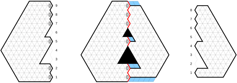
Figure 23. Decomposition of $H^{\prime}_{\mathbf{l}}(a,b,k)$ for $a=5$, $b=6$, $k=6$, and ${\mathbf{l}}=(1,2,5,7,8,9)$ using one of the zigzag lines. The two subregions are (up to reflection) $R_{\emptyset,{\mathbf{l}}}((a+k-1)/2)$ (left) and $\bar{R}_{{\mathbf{l}}-1,\emptyset}((a-1)/2)$ (right).

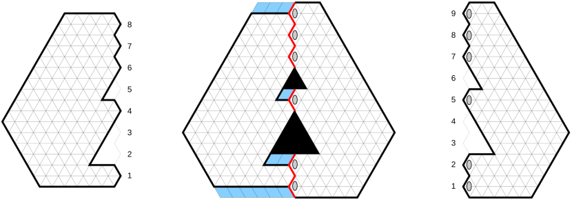
Figure 24. Decomposition of $H^{\prime}_{\mathbf{l}}(a,b,k)$ for $a=5$, $b=6$, $k=6$, and ${\mathbf{l}}=(1,2,5,7,8,9)$ using another of the zigzag line then Figure 15. The two subregions are (up to reflection) $\bar{R}_{{\mathbf{l}}-1,\emptyset}((a+1)/2)$ (right) and $R_{\emptyset,{\mathbf{l}}}((a+k-3)/2)$ (left).

Thus, by Theorem 2.2, $\operatorname{M}(H)=\operatorname{M}(H^{\prime}_{\mathbf{l}}(a,b,k))$ can be expressed as

$$2^{w_{l^{\prime}}(H)-1}(\operatorname{M}(R_{\emptyset,{\mathbf{l}}}((a+k-1)/2))\operatorname{M}(\bar{R}_{{\mathbf{l}}-1,\emptyset}((a-1)/2))+\operatorname{M}(R_{\emptyset,{\mathbf{l}}}((a+k-3)/2))\operatorname{M}(\bar{R}_{{\mathbf{l}}-1,\emptyset}((a+1)/2))).$$ (4.22)

On the other hand, by Lemma 4.4, we have

$$\frac{\operatorname{M}(R_{\emptyset,{\mathbf{l}}}((a+k-1)/2))}{\operatorname{M}(R_{\emptyset,{\mathbf{l}}}((a+k-3)/2))}= \frac{P_{\emptyset,{\mathbf{l}}}((a+k-1)/2)}{P_{\emptyset,{\mathbf{l}}}((a+k-3)/2)}$$ (4.23)

$$= \frac{(a+k-1)!(a+2b+k)!}{(a+b+k-1)!(a+b+k)!}\cdot\prod_{i=1}^{b}\Bigg{[}\frac{(a+k-3)/2+l_{i}+1}{(a+k-3)/2-l_{i}+b+2}\Bigg{]}$$

$$= \frac{(a+k-1)!(a+2b+k)!}{(a+b+k-1)!(a+b+k)!}\cdot\prod_{i=1}^{b}\Bigg{[}\frac{a+k+2l_{i}-1}{a+2b+k-2l_{i}+1}\Bigg{]}$$

and

$$\frac{\operatorname{M}(\bar{R}_{{\mathbf{l}}-1,\emptyset}((a+1)/2))}{\operatorname{M}(\bar{R}_{{\mathbf{l}}-1,\emptyset}((a-1)/2)))}= \frac{\bar{P}_{{\mathbf{l}}-1,\emptyset}((a+1)/2)}{\bar{P}_{{\mathbf{l}}-1,\emptyset}((a-1)/2))}$$ (4.24)

$$= \frac{(a+2l_{b}-2)!(a+2l_{b}-2b+1)!}{(a+2l_{b}-b-1)!(a+2l_{b}-b)!}\prod_{i=1}^{b-1}\Bigg{[}\frac{(a-1)/2+l_{b}+l_{i+1}-b}{(a-1)/2+l_{b}-l_{i+1}+1}\Bigg{]}$$

$$= \frac{(a+2l_{b}-2)!(a+2l_{b}-2b+1)!}{(a+2l_{b}-b-1)!(a+2l_{b}-b)!}\prod_{i=1}^{b-1}\Bigg{[}\frac{a+2l_{b}+2l_{i+1}-2b-1}{a+2l_{b}-2l_{i+1}+1}\Bigg{]}$$

$$= \frac{(a+2b+k-2)!(a+k+1)!}{(a+b+k-1)!(a+b+k)!}\prod_{i=1}^{b-1}\Bigg{[}\frac{a+k+2l_{i+1}-1}{a+2b+k-2l_{i+1}+1}\Bigg{]}$$

Therefore, if we use the two equalities above and the fact that $l_{1}=1$, then we have

$$\frac{\operatorname{M}(R_{\emptyset,{\mathbf{l}}}((a+k-1)/2))\operatorname{M}(\bar{R}_{{\mathbf{l}}-1,\emptyset}((a-1)/2))}{\operatorname{M}(R_{\emptyset,{\mathbf{l}}}((a+k-3)/2))\operatorname{M}(\bar{R}_{{\mathbf{l}}-1,\emptyset}((a+1)/2))} =\frac{(a+k-1)!}{(a+k+1)!}\cdot\frac{(a+2b+k)!}{(a+2b+k-2)!}\cdot\frac{a+k+1}{a+2b+k-1}$$ (4.25)

$$=\frac{a+2b+k}{a+k}.$$

This implies that, if we factor out $\operatorname{M}(R_{\emptyset,{\mathbf{l}}}((a+k-3)/2))\operatorname{M}(\bar{R}_{{\mathbf{l}}-1,\emptyset}((a+1)/2))$ from (4.24), we obtain

$$\operatorname{M}(H)=\operatorname{M}(H^{\prime}_{\mathbf{l}}(a,b,k)) =2^{w_{l^{\prime}}(H)-1}\Bigg{[}\frac{a+2b+k}{a+k}+1\Bigg{]}\operatorname{M}(R_{\emptyset,{\mathbf{l}}}((a+k-3)/2))\operatorname{M}(\bar{R}_{{\mathbf{l}}-1,\emptyset}((a+1)/2))$$ (4.26)

$$=\frac{2a+2b+2k}{a+k}\cdot 2^{w_{l^{\prime}}(H)-1}\operatorname{M}(R_{\emptyset,{\mathbf{l}}}((a+k-3)/2))\operatorname{M}(\bar{R}_{{\mathbf{l}}-1,\emptyset}((a+1)/2))$$

$$=\frac{a+b+k}{a+k}\cdot 2^{w_{l^{\prime}}(H)}\operatorname{M}(R_{\emptyset,{\mathbf{l}}}((a+k-3)/2))\operatorname{M}(\bar{R}_{{\mathbf{l}}-1,\emptyset}((a+1)/2)).$$

On the other hand, if we factor out $\operatorname{M}(R_{\emptyset,{\mathbf{l}}}((a+k-1)/2))\operatorname{M}(\bar{R}_{{\mathbf{l}}-1,\emptyset}((a-1)/2))$ from (4.24), then we have

$$\operatorname{M}(H)=\operatorname{M}(H^{\prime}_{\mathbf{l}}(a,b,k)) =2^{w_{l^{\prime}}(H)-1}\Bigg{[}\frac{a+k}{a+2b+k}+1\Bigg{]}\operatorname{M}(R_{\emptyset,{\mathbf{l}}}((a+k-1)/2))\operatorname{M}(\bar{R}_{{\mathbf{l}}-1,\emptyset}((a-1)/2))$$ (4.27)

$$=\frac{2a+2b+2k}{a+2b+k}\cdot 2^{w_{l^{\prime}}(H)-1}\operatorname{M}(R_{\emptyset,{\mathbf{l}}}((a+k-1)/2))\operatorname{M}(\bar{R}_{{\mathbf{l}}-1,\emptyset}((a-1)/2))$$

$$=\frac{a+b+k}{a+2b+k}\cdot 2^{w_{l^{\prime}}(H)}\operatorname{M}(R_{\emptyset,{\mathbf{l}}}((a+k-1)/2))\operatorname{M}(\bar{R}_{{\mathbf{l}}-1,\emptyset}((a-1)/2)).$$

This completes the proof of the case when $k$ even, $a$ odd, and $l_{1}=1$. The proof of the remaining cases is exactly the same: we apply Theorem 2.2 to $\operatorname{M}(H)$, use Lemma 4.4, and finally use some identities that the indices satisfy (which we can obtain by using the fact that the region consists of the same number of up- and down-pointing unit triangles or by expressing the same length in two different ways; for example, when $k$ even, $a$ odd, and $l_{1}=1$, we had $m=b$ and $l_{m}=l_{b}=b+\frac{k}{2}$).

5. Nearly symmetric hexagons with a shamrock or fern hole

The enumeration of lozenge tilings of hexagons with holes has been studied intensively in last three decades. In particular, many authors considered hexagonal regions with holes near their center because the number of lozenge tilings of such regions behave nicely compared to the cases where holes are away from the center. For example, in [9], the authors found an explicit product formula that enumerates the lozenge tilings of hexagonal regions with triangular holes of arbitrary size removed from their center. This result was then generalized in several different directions. One direction was to deform the triangular holes and find the number of lozenge tilings of hexagonal regions with the new shapes of holes. One such generalization was shown in [12] by the second author and Krattenthaler. In [12], they considered a configuration called shamrock, which can be obtained from a triangle by adding three more triangles touching at vertices, as shown in the picture on the left in Figure 25. Then, they enumerated the number of lozenge tilings of a hexagon with a shamrock removed from the center (this region is called a S-cored hexagon. See the right picture in Figure 25).

Figure 25. A shamrock consisting of four triangles of size $2$, $5$, $7$, and $6$ (left) and an $S$-cored hexagon (right).

The second author then considered symmetry classes of lozenge tilings of a hexagon with a shamrock removed. In particular, in [8], he considered a symmetric hexagon with a symmetric fern removed from along the vertical symmetry axis at any height and enumerated lozenge tilings that are invariant under reflection across the vertical axis (see the left picture in Figure 26). As a byproduct, he also found a closed-form expression that counts the number of lozenge tilings of any such regions with no symmetry required on tilings. This result was also independently found by Lai and Rohatgi in [28]. Later, Lai noticed that when one shifts the symmetric shamrock half a unit unit away from the vertical symmetry axis (by translating the shamrock one unit in the southeast or northeast direction; see the right picture in Figure 26), then the prime factorization of the number of lozenge tilings of the new region consists of small prime numbers, which is a good indication of the existence of a simple product formula.

Figure 26. A symmetric hexagon with a symmetric shamrock removed from along the symmetry axis (left) and the same region with the shamrock shifted one unit southeast (right).

The reader might have already noticed that the situation of the current section is very similar to that of subsection 4.5. Indeed, Theorem 2.2 can be applied to a symmetric hexagon with a shamrock hole shifted one unit southeast from a symmetric position. If one splits the region using the two zigzag lines of Theorem 2.2, one gets four subregions whose tiling generating functions were determined in [8] and [28]. Thus, we can use those formulas and Theorem 2.2 to find formulas that enumerate the lozenge tilings of our desired regions, solving this way Lai’s second open problem.

We point out that there is also another, conceptual justification for why the number of lozenge tilings of these regions is given by a simple product formula.

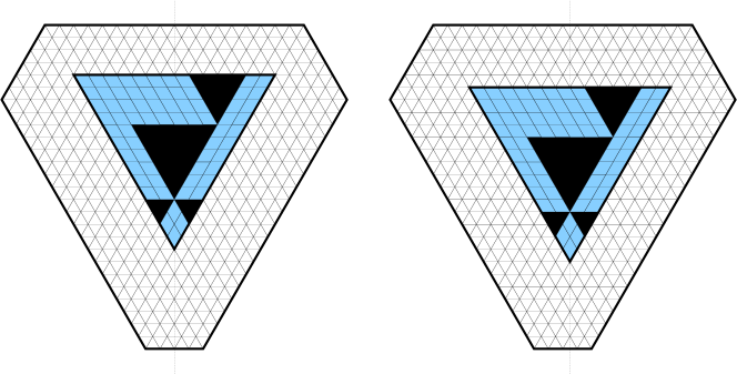
Figure 27. Regions that we can obtain by applying the bowtie squeezing theorem to the regions in Figure 26. If we flip these pictures upside down, the left picture and the right picture become the regions whose number of lozenge tilings were given by Theorem 4.1 and Theorem 4.2, respectively.

This employs a result of the second author, Lai, and Rohatgi [13] called the “bowtie squeezing theorem”. This theorem provides a simple product formula for the ration between the number of lozenge tilings of two regions that are connected via a certain “bowtie squeezing” operation (see [13] for more details about this operation.). If one applies this bowtie squeezing in a convenient way to a symmetric hexagon with a symmetric shamrock removed, then one can get another symmetric hexagon with a triangle removed, where the side length of the triangle is the sum of the side lengths of each of the four triangles that constitute the shamrock (compare the pictures in Figure 26 and 27).

In particular, if we apply this theorem to a hexagonal region with a symmetric shamrock removed from a vertical axis that is half a unit away from the vertical symmetry axis, then the ratio between the number of lozenge tilings of the region and that of the counterpart region, which is a symmetric hexagon with a triangle removed along the vertical axis half a unit away from the symmetry axis, is given by a simple product formula by the bowtie squeezing theorem. However, since the latter region is a region whose number of lozenge tilings is provided by Theorem 4.2, the former (the number of lozenge tilings of a symmetric hexagon with a symmetric shamrock removed half a unit away from its symmetry axis) is also given by a simple product formula. As in the previous section, given a symmetric hexagon, let $\ell$ and $\ell^{\prime}$ be the vertical symmetry axis and a vertical line that is half-unit away from $\ell$. From this discussion, we can deduce the following theorem, which solves Lai’s second open problem.

Theorem 5.1.

The number of lozenge tilings of a symmetric hexagon with a symmetric shamrock removed from $\ell^{\prime}$ at any height is given by a simple product formula.

Figure 28. A fern consisting of five triangles of size $1,2,5,3,$ and $4$, left to right (left) and an $F$-cored hexagon (right).

One can use a similar argument to find another family of regions whose number of lozenge tilings is given by simple product formulas. In [7], the second author defined a structure called a fern, which is a collection of an arbitrary number of contiguous triangles of alternating orientations that are lined up along a common axis (see the left picture in Figure 28), and enumerated the number of lozenge tilings of a hexagon with a fern removed from the center (such a region is called a F-cored hexagon; see the right picture in Figure 28). Motivated by Lai’s previously discussed conjectures, it is natural to consider a symmetric hexagon with a symmetric fern removed from along the symmetry axis, or from along an axis that is half a unit away from the symmetry axis of the hexagon.

Figure 29. A symmetric hexagon with a symmetric fern removed from along the symmetry axis (left) and the same region with the fern shifted one unit southeast (right).

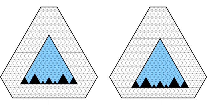
Figure 30. Regions obtained by applying the shuffling theorem to the regions in Figure 29. The number of lozenge tilings of the left and the right regions are given by Theorem 4.1 and 4.2, respectively.

We claim that the number of lozenge tilings of these two regions are also given by simple product formulas. This time, one can apply shuffling theorem of Lai and Rohatgi [29] to these regions. This shuffling theorem can be used to obtain simple expressions for the ratio between the number of lozenge tilings of a symmetric hexagon with a symmetric fern removed from along its symmetry axis and that of a corresponding region, which is a symmetric hexagon with a triangle removed from along its symmetry axis (compare pictures on the left in Figures 29 and 30). Similarly, the theorem also gives simple expressions connecting two similar regions with holes shifted one unit in the southeast direction (compare the pictures on the right in Figures 29 and 30). However, again, the number of lozenge tilings of a symmetric hexagon with a triangle removed from along its symmetry axis (or a vertical axis half a unit away from the symmetry axis) is given by Theorem 4.1 (or Theorem 4.2/4.3). Thus, this implies that the numbers of lozenge tilings of these two regions are given by simple product formulas (and thus only contain relatively small prime factors in their prime factorizations). Furthermore, one can also obtain concrete product formulas by combining the shuffling theorem and Theorem Theorem 4.2. Again, based on the discussion in this paragraph, we can obtain the following theorem. We continue to use $\ell$ and $\ell^{\prime}$ to denote the symmetry axis of symmetric hexagons and a vertical line half a unit away from $\ell$.

Theorem 5.2.

The number of lozenge tilings of a symmetric hexagon with a symmetric fern removed from $\ell$ or $\ell^{\prime}$ at any height is given by a simple product formula. As a result, the prime factorization of the number of lozenge tilings of these regions consists of small prime factors.

Remark $4$. The fact that the number of lozenge tilings of a vertically symmetric hexagon with a shamrock or fern removed from along $\ell$ or $\ell^{\prime}$ is given by simple product formula also follows using the first author’s snowflake flipping Theorem [2].

Figure 31. Symmetric hexagons with intrusions along the symmetry axis (top) and half-unit shifted intrusions (bottom).

The idea of the proof that we used in the previous section can also be used in many other lozenge tiling enumeration problems. For example, consider a symmetric hexagon, which has both a vertical and a horizontal symmetry axis, and denote its vertical symmetry axis by $\ell$. Remove any even number of consecutive unit triangles along $\ell$ starting from the bottom (see the two top figures Figure 31. The regions look different, depending on the parity of the bottom sides). This region was called a symmetric hexagon with an intrusion, and the product formulas that count the number of lozenge tilings of these regions were proved in [1] using an idea from [11]. The proof again used the factorization theorem for matchings, together with a result of the second author, which was presented in subsection 4.3. One can then consider a similar problem, by considering the same symmetric hexagon and a vertical axis $\ell^{\prime}$, which is obtained from $\ell$ by shifting it half a unit to the right, and removing any even number of consecutive unit triangles from along $\ell^{\prime}$ starting from the bottom (see the two bottom figures in Figure 31). The same question can be asked about the number of lozenge tilings of this symmetric hexagonal region with a half-unit shifted intrusion. This problem can also be solved using Theorem 2.2 and Lemma 4.4. Indeed, if one divides the new region using the two zigzag lines of Theorem 2.2, then the resulting regions belong to one of the family of regions introduced in subsection 4.2 and we can again use Lemma 4.4 to simplify the expression, as we showed in subsection 4.5. The same idea can also be used to answer the same question when a more general intrusion (considered by the first author and Lai in [4]) is removed from a symmetric hexagon.

It turns out that our technique can also be used to find the number of lozenge tilings of certain nearly symmetric hexagonal regions with holes that are not given by simple product formulas. We present one such instance in the next section.

6. Nearly symmetric hexagons with a lozenge hole

Using Theorem 2.2, we can also obtain a counterpart of a result of Fulmek and Krattenthaler which was presented in [19]. In [19] and [20], these authors considered the problem of enumerating lozenge tilings of a hexagon that has both vertical and horizontal symmetry — we will call this a symmetric hexagon — which contain a fixed lozenge (or equivalently, tilings of a hexagon with a lozenge shaped hole). In [19], they considered a symmetric hexagon, fixed a unit lozenge on the vertical symmetry axis in an arbitrary position, and they proved the following two results (Figure 32 illustrates the two types of regions they considered).

Figure 32. The regions Fulmek and Krattenthaler considered in [19]. These two pictures illustrate the case when $m=2$, $N=6$, and $l=2$.

Theorem 6.1 (Theorem 1 in [19]).

Let $m$ be a nonnegative integer and $N$ be a positive integer. The number of lozenge tilings of a hexagon with sides $N,2m,N,N,2m,N$, which contain the $l$-th lozenge on the symmetry axis which cuts through the sides of length $2m$, equals

$$\frac{m\binom{m+N}{m}\binom{m+N-1}{m}}{\binom{2m+2N-1}{2m}}\Bigg{(}\sum_{e=0}^{l-1}(-1)^{e}\binom{N}{e}\frac{(N-2e)(\frac{1}{2})_{e}}{(m+e)(m+N-e)(\frac{1}{2}-N)_{e}}\Bigg{)}\cdot\prod_{i=1}^{N}\prod_{j=1}^{N}\prod_{k=1}^{2m}\frac{i+j+k-1}{i+j+k-2}.$$ (6.1)

Theorem 6.2 (Theorem 2 in [19]).

Let $m$ and $N$ be positive integers. The number of lozenge tilings of a hexagon with sides $N+1,2m-1,N+1,N+1,2m-1,N+1$, which contain the $l$-th lozenge on the symmetry axis which cuts through the sides of length $2m-1$, equals

$$\frac{m\binom{m+N}{m}\binom{m+N-1}{m}}{\binom{2m+2N-1}{2m}}\Bigg{(}\sum_{e=0}^{l-1}(-1)^{e}\binom{N}{e}\frac{(N-2e)(\frac{1}{2})_{e}}{(m+e)(m+N-e)(\frac{1}{2}-N)_{e}}\Bigg{)}\cdot\prod_{i=1}^{N+1}\prod_{j=1}^{N+1}\prod_{k=1}^{2m-1}\frac{i+j+k-1}{i+j+k-2}.$$ (6.2)

In [20], Fulmek and Krattenthaler considered the enumeration of lozenge tilings of the same symmetric hexagon with a unit lozenge fixed on the horizontal symmetry axis. Unlike their result in [19], they considered three cases in which the fixed lozenge is 1) half a unit, 2) one unit, or 3) one and half a unit away from the vertical symmetry axis. We recall the two theorems in [20] that correspond to the first case (see the two pictures in Figure 33 that illustrate the regions considered).

Figure 33. The regions Fulmek and Krattenthaler considered in [20]. These pictures illustrate the case when $m=2$ and $n=3$.

Theorem 6.3.

(Theorem 1 in [20]) Let $n$ and $m$ be positive integers. The number of lozenge tilings of a hexagon with side lengths $2n,2m,2n,2n,2m,2n,$ which contain the lozenge just to the right of the center of the hexagon, equals

$$\frac{nm\binom{2n}{n}\binom{2n-1}{n}\binom{2m}{m}}{\binom{4n+2m-1}{2n+m}}\Bigg{(}-\frac{1}{(n+m)^{2}} +\frac{4n+2}{(n+1)(2n-1)(n+m-1)(n+m+1)}$$ (6.3)

$$\cdot\sum_{h=0}^{n-1}\frac{(2)_{h}(1-n)_{h}(\frac{3}{2}+n)_{h}(1-n-m)_{h}(1+n+m)_{h}}{(1)_{h}(2+n)_{h}(\frac{3}{2}-n)_{h}(2+n+m)_{h}(2-n-m)_{h}}\Bigg{)}$$

$$\cdot\prod_{i=1}^{2n}\prod_{j=1}^{2m}\prod_{k=1}^{2n}\frac{i+j+k-1}{i+j+k-2}.$$

Theorem 6.4.

(Theorem 2 in [20]) Let $n$ be a positive integer and $m$ be a positive integer. The number of lozenge tilings of a hexagon with side lengths $2n+1,2m-1,2n+1,2n+1,2m-1,2n+1,$ which contain the lozenge just to the right of the center of the hexagon, equals

$$\frac{(n+1)m\binom{2n}{n}\binom{2n+1}{n}\binom{2m-1}{m}}{\binom{4n+2m}{2n+m}}\Bigg{(}\frac{1}{(n+m)^{2}} +\frac{4n}{(n+1)(2n-1)(n+m-1)(n+m+1)}$$ (6.4)

$$\cdot\sum_{h=0}^{n-1}\frac{(2)_{h}(1-n)_{h}(\frac{3}{2}+n)_{h}(1-n-m)_{h}(1+n+m)_{h}}{(1)_{h}(2+n)_{h}(\frac{3}{2}-n)_{h}(2+n+m)_{h}(2-n-m)_{h}}\Bigg{)}$$

$$\cdot\prod_{i=1}^{2n+1}\prod_{j=1}^{2m-1}\prod_{k=1}^{2n+1}\frac{i+j+k-1}{i+j+k-2}.$$

Note that given a region $R$ and a lozenge $L$ inside the region, lozenge tilings of $R$ containing $L$ can be identified with lozenge tilings of the region obtained from $R$ by creating a lozenge-shaped hole at location $L$. Thus, the four theorems above can be regarded as lozenge tiling enumerations of symmetric hexagons with unit lozenges removed.

The result we present in this section can be considered as hybrid of the above theorems. For a nonnegative integer $m$ and a positive integer $N$, let $V(N,2m,l)$ be the region obtained from the symmetric hexagon of side-lengths $2m,N,N,2m,N,N$ (clockwise from top) by deleting the $l$-th lozenge on the vertical symmetry axis. Similarly, let $V^{\prime}(N,2m,l)$ be the region obtained from the same hexagon by deleting the $l$-th lozenge on the vertical axis that is half a unit to the right of the vertical symmetry axis.

Similarly, for positive integers $m$ and $N$, let $V(N+1,2m-1,l)$ be the region obtained from the symmetric hexagon of side-lengths $2m-1,N+1,N+1,2m-1,N+1,N+1$ (clockwise from top) by deleting the $l$-th lozenge on the vertical symmetry axis. Similarly, let $V^{\prime}(N+1,2m-1,l)$ be the region obtained from the same hexagon by deleting the $l$-th lozenge on the vertical axis that is half a unit to the right of the vertical symmetry axis.

The first two results of Fulmek and Krattenthaler stated above (Theorem 6.1 and 6.2) are about the number of lozenge tilings of the regions $V(N,2m,l)$ and $V(N+1,2m-1,l)$. The main results of this section (see Theorems 6.5 and 6.6 below) give formulas for the number of lozenge tilings of the regions $V^{\prime}(N,2m,l)$ and $V^{\prime}(N+1,2m-1,l)$, and thus extends the results of Fulmek and Krattenthaler quoted as Theorems 6.3 and 6.4 by lending them the generality of the context of their results quoted as Theorems 6.1 and 6.2.

Figure 34. The regions considered in the current section. These two pictures illustrate $V^{\prime}(N,2m,l)$ and $V^{\prime}(N-1,2m+1,l)$ when $m=2$, $N=6$, and $l=2$.

Theorem 6.5.

Let $m$ be a positive integer and $N$ be a positive integer greater than $1$. The number of lozenge tilings of the region $V^{\prime}(N,2m,l)$ obtained from the hexagon with sides $2m,N,N,2m,N,N$ $($clockwise from top$)$ by deleting the $l$-th lozenge from the top on the vertical axis half a unit away from the vertical symmetry axis, is given by

$$\operatorname{M}(V^{\prime}(N,2m,l))=\frac{(m+1)_{N}(m)_{N}(N)_{N-1}}{(2m+1)_{N}(2m+N)_{N}(N-1)!}\cdot\sigma_{1}(N,m,l)\cdot\prod_{i=1}^{N}\prod_{j=1}^{N}\prod_{k=1}^{2m}\frac{i+j+k-1}{i+j+k-2}$$ (6.5)

where

$$\sigma_{1}(N,m,l)= (2m+2N-1)\cdot\sum_{e=0}^{l-1}(-1)^{e}\binom{N-1}{e}\frac{(N-2e-1)(\frac{1}{2})_{e}}{(m+e)(m+N-e-1)(\frac{3}{2}-N)_{e}}$$ (6.6)

$$+ (2m+1)\cdot\sum_{e=0}^{l-1}(-1)^{e}\binom{N-1}{e}\frac{(N-2e-1)(\frac{1}{2})_{e}}{(m+e+1)(m+N-e)(\frac{3}{2}-N)_{e}}.$$

Theorem 6.6.

Let $m$ be a nonnegative integer and $N$ be a positive integer greater than $1$. The number of lozenge tilings of the region $V^{\prime}(N-1,2m+1,l)$ obtained from the hexagon of sides $2m+1,N-1,N-1,2m+1,N-1,N-1$ $($clockwise from top$)$ by deleting the $l$-th lozenge from the top on the vertical axis half a unit away from the vertical symmetry axis, is given by

$$\operatorname{M}(V^{\prime}(N-1,2m+1,l))=\frac{(m+1)_{N-1}(m+1)_{N-1}(N-1)_{N-1}}{(2m+2)_{N-1}(2m+N)_{N-1}(N-1)!}\cdot\sigma_{2}(N,m,l)\cdot\prod_{i=1}^{N-1}\prod_{j=1}^{N-1}\prod_{k=1}^{2m+1}\frac{i+j+k-1}{i+j+k-2}$$ (6.7)

where

$$\sigma_{2}(N,m,l)= m\cdot\sum_{e=0}^{l-1}(-1)^{e}\binom{N-1}{e}\frac{(N-2e-1)(\frac{1}{2})_{e}}{(m+e)(m+N-e-1)(\frac{3}{2}-N)_{e}}$$ (6.8)

$$+ (m+N)\cdot\sum_{e=0}^{l-1}(-1)^{e}\binom{N-1}{e}\frac{(N-2e-1)(\frac{1}{2})_{e}}{(m+e+1)(m+N-e)(\frac{3}{2}-N)_{e}}.$$

We deduce the above two results from Theorem 2.2, using also enumeration results on certain families of regions given in [19]. Although one of them is a special case of a region we considered in an earlier section, for consistency with [19] we use the notation from there.

For nonnegative integers $m$ and $N$, let $S(N,m)$ be the pentagonal region depicted on the left in Figure 35; note that this region was previously denoted by $\overline{R}_{(1,\ldots,N),\emptyset}(m)$ in subsection 4.2. Also, for a nonnegative integer $m$ and positive integers $l$ and $N$ such that $l\leq N$, we define the region $C(N,m,l)$ as follows: on $S(N,m)$, we label the $N$ rightmost vertical lozenges by $1,\ldots,N$, from top to bottom. Then we remove the vertical lozenge labeled by $l$ and assign the weight $\frac{1}{2}$ to the remaining $N-1$ vertical lozenges (see the picture on the right in Figure 35). In [19], Fulmek and Krattenthaler provided the number of lozenge tilings for $S(N,m)$ and the weighted count of lozenge tilings of $C(N,m,l)$.

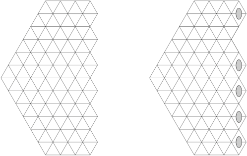
Figure 35. Left. The region $S(N,m)$ for $N=6$ and $m=3$. Right. The region $C(N,m,l)$ for $N=6$, $m=3$ and $l=2$. Lozenges marked by ellipses are weighted by $\frac{1}{2}$, as in the previous sections.

Lemma 6.7.

$((2.4)$ and $(2.6)$ in [19]$)$ For any nonnegative integer $m$ and positive integer $N$,

$$\operatorname{M}(S(N,m))=\prod_{i=1}^{N}\frac{(N+m-i+1)!(i-1)!(2m+i+1)_{i-1}}{(m+i-1)!(2N-2i+1)!}.$$ (6.9)

Lemma 6.8.

$((2.5)$ and $(2.7)$ in [19]$)$ For any nonnegative integer $m$ and positive integers $l$ and $N$ such that $l\leq N$,

$$\operatorname{M}(C(N,m,l))=\frac{(m)_{N+1}}{2^{N-1}N!}\prod_{i=1}^{\lfloor\frac{N}{2}\rfloor}\frac{(2m+2i)_{2N-4i+1}}{(2i)_{2N-4i+1}}\cdot\sum_{e=0}^{l-1}(-1)^{e}\binom{N}{e}\frac{(N-2e)(\frac{1}{2})_{e}}{(m+e)(m+N-e)(\frac{1}{2}-N)_{e}}.$$ (6.10)

[Proof of Theorem 6.6] We apply Theorem 2.2 to the region $V^{\prime}(N,2m,l)$. To do that, we split the region using the two different zigzag lines along the vertical axis through the hole. While one of the zigzag lines splits the region into $S(N,m)$ and $C(N-1,m,l)$, the other zigzag line splits the region into $S(N,m-1)$ and $C(N-1,m+1,l)$ (see the two pictures in Figure 36). Thus, by Theorem 2.2, we have

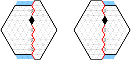
Figure 36. One of the two zigzag lines splits $V^{\prime}(4,6,2)$ into the two sub regions $C(5,3,2)$ and $S(6,1)$ (left). The other zigzag line splits the same region into the two subregions $C(5,2,2)$ and $S(6,2)$ (right).

$$\operatorname{M}(V^{\prime}(N,2m,l))=2^{N-2}\Big{[}\operatorname{M}(S(N,m))\operatorname{M}(C(N-1,m,l))+\operatorname{M}(S(N,m-1))\operatorname{M}(C(N-1,m+1,l))\Big{]}.$$ (6.11)

By combining (6.9), (6.10), (6.11) and factoring out some common factors, we get the desired formula for $\operatorname{M}(V^{\prime}(N,2m,l))$.

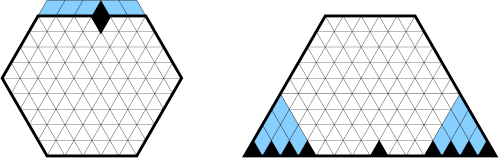
Figure 37. If we remove the forced lozenges from the region $V^{\prime}(N,m,1)$ on the left (here $N=5$ and $m=5$), and also from the region on the right (which is a special case of the regions whose tilings are enumerated by Proposition 2.1 of [14]), the two resulting regions are congruent.

[Proof of Theorem 6.8] We first consider the case when $l=1$. In this case, the region $V^{\prime}(N-1,2m+1,1)$ can be regarded as a trapezoid region with dents on its base (see two pictures in Figure 37 and the explanation in the caption). The number of lozenge tilings of such regions was given in [14, Proposition 2.1] and one can check that the $l=1$ specialization of our claimed formula agrees with the expression obtained using[14, Proposition 2.1]. Assume therefore that $l\geq 2$, and apply Theorem 2.2. To do that, we again consider two zigzag lines along the vertical line through the hole. One of the zigzag lines divides the region into $S(N-2,m)$ and $C(N-1,m+1,l)$, while the other divides it into $S(N-2,m+1)$ and $C(N-1,m,l)$ (see the two pictures in Figure 38. Thus, by Theorem 2.2, we obtain

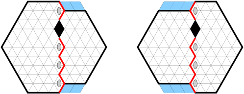
Figure 38. One of the two zigzag lines splits $V^{\prime}(5,5,2)$ into the two sub regions $C(5,3,2)$ and $S(4,2)$ (left). The other zigzag line splits the same region into the two subregions $C(5,2,2)$ and $S(4,3)$ (right).

$$\operatorname{M}(V^{\prime}(N-1,2m+1,l))$$ (6.12)

$$= 2^{N-3}\Big{[}\operatorname{M}(S(N-2,m))\operatorname{M}(C(N-1,m+1,l))+\operatorname{M}(S(N-2,m+1))\operatorname{M}(C(N-1,m,l))\Big{]}.$$

Using (6.9), (6.10), (6.12) and factoring out some common factors, we get the claimed formula for $\operatorname{M}(V^{\prime}(N+1,2m-1,l))$.

7. Aztec rectangles with collinear unit holes

Let $m$ and $n$ be positive integers with $m\leq n$. The $m\times n$ Aztec rectangle, denoted by $AR(m,n)$, is the region consisting of all unit squares on $\mathbb{Z}^{2}$ whose centers $(x,y)$ satisfy the inequalities $|x|+|y|\leq n$ and $x+y\geq n-2m$. In this section, we rotate the region $AR(m,n)$ by $45^{\circ}$ in counterclockwise direction (see the pictures in Figure 39; at this point, ignore the black unit squares in the pictures).

Unless $m=n$ (when it becomes the Aztec diamond $AD_{n}$), the Aztec rectangle $AR(m,n)$ does not have any domino tilings: it is not hard to check that if we chessboard color the square grid, $AR(m,n)$ has $n-m$ more unit squares of one color than the other. This can be fixed as follows. Label the bottommost unit squares in $AR(m,n)$ by $1,\ldots,n$ from left to right. For any subset $S\subseteq[n]\coloneqq\{1,\ldots,n\}$ of size $m$, we delete the unit squares labeled with elements of $[n]\setminus S$ from $AR(m,n)$, and denote the resulting region by $AR(m,n:S)$ (see the picture on the left in Figure 39 for an illustration). Then the region $AR(m,n:S)$ always admits domino tilings; the number of them is given by (see [5],[18],[30])

$$\\ M(AR(m,n;S))=2^{m(m+1)/2}\prod_{1\leq i<j\leq m}\frac{s_{j}-s_{i}}{j-i},$$ (7.1)

where $S=\{s_{1},\ldots,s_{m}\}$, with $s_{1}<\cdots<s_{m}$.

Figure 39. The regions $AR(4,7;\{1,2,4,6\})$ (left) and $\overline{AR}(4,7;\{2,3,5,7\})$ (right). Both regions are obtained from $AR(4,7)$ by deleting some unit squares.

Next, for any subset $T=\{t_{1},\ldots,t_{m}\}\subseteq\{n+1\}$ of size $m$ (again, with elements of $T$ written in increasing order), consider the region $\overline{AR}(m,n:T)$ defined as follows. From $AR(m,n)$, remove the $n$ unit squares at the bottom. Note that the resulting region has $n+1$ unit squares on the (new) bottom. Label the unit squares at the bottom of the new region by $1,\ldots,n+1$ from left to right. Finally, delete the unit squares labeled by elements of $T$, and denote the resulting region by $\overline{AR}(m,n:T)$. The number of domino tilings for this region was studied in [18] and [21], and is given by the following product formula

$$\operatorname{M}(\overline{AR}(m,n;T))=2^{m(m-1)/2}\prod_{1\leq i<j\leq m}\frac{t_{j}-t_{i}}{j-i},$$ (7.2)

In [5], the second author proved that if an arbitrary collection of unit squares is deleted from the horizontal symmetry axis of an Aztec rectangle, the number of domino tilings of the resulting region is given by a simple product formula. More precisely, let $m$ and $N$ be positive integers with $2m\leq N$. Then the number of domino tilings of a $2m\times N$ Aztec rectangle, where all the unit squares on the central horizontal row, except the $t_{1}$-st, the $t_{2}$-nd,$\ldots$, and the $t_{2m}$-th unit square, have been removed equals

$$\frac{2^{m^{2}+2m}}{\displaystyle\prod_{i=1}^{m}(i-1)!^{2}}\prod_{1\leq i<j\leq m}(t_{2j}-t_{2i})\prod_{1\leq i<j\leq m}(t_{2j-1}-t_{2i-1}).$$ (7.3)

This was generalized by Krattenthaler [23], who considered the following general problem: if we delete collinear unit squares along an arbitrary horizontal line from an Aztec rectangle, what is the number of domino tilings of the resulting regions? Using certain Schur function identities, he answered this question by finding some explicit formulas.

As proved in [5] (see also [21]), the special case when the horizontal axis containing the deleted unit squares is the symmetry axis, this formula becomes a simple product formula. Furthermore, the special case of Krattenthaler’s formula when the line containing the deleted squares is just below the symmetry axis also turns out to be a simple product formula.

Figure 40. A picture that illustrates Theorem 7.1 with $m=2$, $N=8$, and $(t_{1},t_{2},t_{3},t_{4},t_{5})=(1,4,5,6,8)$ (left) and another picture that illustrates Theorem 7.2 with $m=5$, $N=7$, and $(t_{1},t_{2},t_{3},t_{4},t_{5})=(1,2,5,6,8)$ (left). Later when we prove Theorem 7.3, the picture on the left is denoted by $R_{1}(2m+1,N;(t_{1},\ldots,t_{2m+1}))=R_{1}(5,8;(1,4,5,6,8))$.

Theorem 7.1 (Theorem 9 in [23]).

Let $m$ and $N$ be positive integers with $2m+1\leq N$. Then the number of domino tilings of a $(2m+1)\times N$ Aztec rectangle, where all the unit squares on the horizontal row that is by $1$ below the central row, except for the $t_{1}$-st, the $t_{2}$-nd,$\ldots$, and the $t_{2m+1}$-th unit square, have been removed $($see the left picture in Figure $\ref{fgc})$, equals

$$\frac{2^{m^{2}+3m+1}}{\displaystyle\prod_{i=1}^{m}(i-1)!\prod_{i=1}^{m+1}(i-1)!}\prod_{1\leq i<j\leq m}(t_{2j}-t_{2i})\prod_{1\leq i<j\leq m+1}(t_{2j-1}-t_{2i-1}).$$ (7.4)

Theorem 7.2 (Theorem 10 in [23]).

Let $m$ and $N$ be positive integers with $2m\geq N$. Then the number of domino tilings of a $2m\times N$ Aztec rectangle, where all the unit squares on the horizontal row that is by $1$ below the central row, except for the $t_{1}$-st, the $t_{2}$-nd,$\ldots$, and the $t_{2N-2m+1}$-th unit square, have been removed $($see the right picture in Figure $\ref{fgc})$, equals

$$2^{m^{2}-m+N}\frac{\displaystyle\prod_{i=m+1}^{N+1}(i-1)!\prod_{i=m+2}^{N+1}(i-1)!}{\displaystyle\prod_{i=1}^{2N-2m+1}(t_{i}-1)!(N+1-t_{i})!}\times\prod_{1\leq i<j\leq N-m}(t_{2j}-t_{2i})\prod_{1\leq i<j\leq N-m+1}(t_{2j-1}-t_{2i-1}).$$ (7.5)

Krattenthaler’s proof of Theorems 7.1–7.2 in [23] was based on certain Schur function identities. In this section, we give a very simple proof of these theorems using Theorem 2.1.

[Proof of Theorems 7.1–7.2]

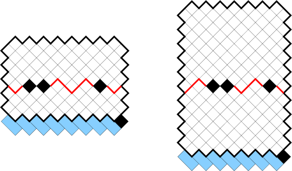
Figure 41. Application of Theorem 2.1(b) to the two regions in Figure 7.1

We first prove Theorem 7.1. To do that, we add one layer at the bottom of the region by adding $2N+1$ unit squares that form a zigzag path. Then, we delete the rightmost newly added unit square (see the left picture in Figure 41). Then, the dual graph of the resulting region is a symmetric graph with a defect, to which Theorem 2.1(b) can be applied. If we apply Theorem 2.1(b) to the dual graph, take dual again, and delete forced dominoes, then the number of domino tilings of the region in Theorem 7.1 can be expressed as follows:

$$2^{m}\operatorname{M}(AR(m+1,N;\{t_{2i-1}\}_{i\in[m+1]}))\operatorname{M}(AR(m,N;\{t_{2i}\}_{i\in[m]})).$$ (7.6)

Combining (7.1) and (7.6), one can get (7.4) and this completes the proof of Theorem 7.1.

The proof of Theorem 7.2 is very similar to that of Theorem 7.1 that we just presented. We add one layer at the bottom of the region by adding $2N+1$ unit squares in the same way as in the proof of Theorem 7.1. We again remove the rightmost unit square among $2N+1$ newly added unit squares (see the right picture in Figure 41). We can again apply Theorem 2.1(b) to the dual graph, take the dual again, and delete forced dominoes. As a result, we have the following factorization of the number of domino tilings of the region in Theorem 7.2.

$$2^{N-m}\operatorname{M}(\overline{AR}(m,N;[N+1]\setminus{\{t_{2i-1}\}}_{i\in[N-m+1]}))\operatorname{M}(\overline{AR}(m+1,N;[N+1]\setminus\{t_{2i}\}_{i\in[N-m]})).$$ (7.7)

Combining (7.2) and (7.7), one gets (7.5), which proves Theorem 7.2.

We finish this section by presenting one more new proof, namely of the following theorem, which is another special case of Krattenthaler’s general result (Theorem 11 in [23]).

Theorem 7.3 (The case $d=2$ in Theorem 11 in [23]).

Let $m$ and $N$ be positive integers with $2m+2\leq N$. Then the number of domino tilings of a $(2m+2)\times N$ Aztec rectangle, where all the unit squares on the horizontal row that is by $2$ below the central row, except for the $t_{1}$-st, the $t_{2}$-nd,$\ldots$, and the $t_{2m+2}$-th unit square, have been removed, equals

$$\frac{2^{m^{2}+4m+3}}{\displaystyle\prod_{i=1}^{m}(i-1)!\prod_{i=1}^{m+2}(i-1)!}\cdot\Bigg{[}\prod_{1\leq i<j\leq m+1}(t_{2j}-t_{2i})(t_{2j-1}-t_{2i-1})\Bigg{]}\cdot\Bigg{(}\sum_{i=1}^{2m+2}(-1)^{i}t_{i}\Bigg{)}.$$ (7.8)

Note that our formula in (7.8) has a simpler form than Krattenthaler’s original formula (see (4.5) in [23]. Although one can set $d=2$ in that formula, it is not so straightforward to see that the second line in that formula equals $\sum_{i=1}^{2m+2}(-1)^{i}t_{i}$). Krattenthaler’s proof of the above theorem used some Schur function identities. On the other hand, we prove this theorem using Kuo’s graphical condensation. Although we stated Kuo’s condensation theorem in Section 2 (see Theorem 2.3), we state here a different version of it, because it is this latter version that we need in our proof of Theorem 7.3.

Theorem 7.4 (Theorem 2.1 in [24]).

Let $G=(V_{1},V_{2},E)$ be a plane bipartite graph in which $|V_{1}|=|V_{2}|$. Let vertices $a,b,c,$ and $d$ appear in a cyclic order on the same face of $G$. If $a,c\in V_{1}$ and $b,d\in V_{2}$, then

$$\operatorname{M}(G)\operatorname{M}(G-\{a,b,c,d\})=\operatorname{M}(G-\{a,c\})\operatorname{M}(G-\{b,d\})+\operatorname{M}(G-\{a,d\})\operatorname{M}(G-\{b,c\}).$$

Let $R_{0}(2m,N;\{t_{1},\ldots,t_{2m}\})$, $R_{1}(2m+1,N;\{t_{1},\ldots,t_{2m+1}\})$, and $R_{2}(2m+2,N;\{t_{1},\ldots,t_{2m+2}\})$ be the regions described just before equation (7.3), in Theorem 7.1, and in Theorem 7.3, respectively. Under this notation, we want to show that the number of domino tilings of $R_{2}(2m+2,N;\{t_{1},\ldots,t_{2m+2}\})$ is given by (7.8). Note that this region the region $R_{2}(2m+2,N;\{t_{1},\ldots,t_{2m+2}\})$ has $N-(2m+2)$ unit square holes in it. This is important because we will use an induction on this quantity.

[Proof of Theorem 7.3]

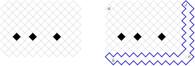
Figure 42. $R_{2}(2m+2,N,\{t_{1},\ldots,t_{2m+2}\})=R_{2}(6,9;\{1,3,5,6,8,9\})$ (left) and $R_{1}(2m+3,N+1;\{t_{1},\ldots,t_{2m+2},N+1\})=R_{1}(7,10,\{1,3,5,6,8,9,10\})$ (right). The right region is obtained from the left region by adding a layer at the bottom and the right side of the left region. In the right picture, the extended part is marked by thick blue lines; four unit squares $a,b,c,$ and $d$ are also marked.

Note that we only have to show Theorem 7.3 for the regions $R_{2}(2m+2,N;\{t_{1},\ldots,t_{2m+2}\})$ with $t_{1}=1$ and $t_{2m+2}=N$. This is because if $t_{1}\neq 1$ or $t_{2m+2}\neq N$, then by deleting some forced dominoes, one can obtain a smaller region with fewer holes in it.

We first construct a recurrence relation using Kuo’s graphical condensation (Theorem 7.4). Consider a region $R_{2}(2m+2,N;\{t_{1},\ldots,t_{2m+2}\})$ with $t_{1}=1$ and $t_{2m+2}=N$. We then add a layer on the bottom and right sides of the region, as described in Figure 42. On this extended region, we choose four unit squares $a,b,c,$ and $d$ as shown in the right picture in Figure 42. The dual graph of the extended region, together with its four vertices corresponding to unit squares labeled by $a,b,c,$ and $d$, satisfies the conditions required in Theorem 7.4. If we apply Kuo’s graphical condensation on the dual graph and take dual again, then we obtain the following recurrence relation (see the six regions in Figure 43):

$$\operatorname{M}(R_{1}(2m+3,N+1;\{t_{1},\ldots,t_{2m+2},N+1\}))\operatorname{M}(R_{1}(2m+1,N-1;\{t_{2}-1,\ldots,t_{2m+2}-1\}))$$ (7.9)

$$= \operatorname{M}(R_{2}(2m+2,N;\{t_{2}-1,\ldots,t_{2m+2}-1,N\}))\operatorname{M}(R_{0}(2m+2,N;\{t_{1},\ldots,t_{2m+2}\}))$$

$$+ \operatorname{M}(R_{2}(2m+2,N;\{t_{1},\ldots,t_{2m+2}\}))\operatorname{M}(R_{0}(2m+2,N;\{t_{2}-1,\ldots,t_{2m+2}-1,N\})).$$

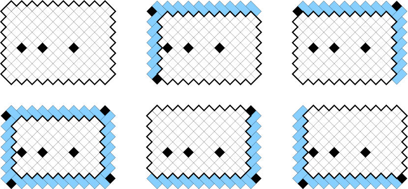
Figure 43. The six regions appearing in the recurrence relation we obtain by applying Kuo’s graphical condensation to the region in the picture on the right in Figure 42.

One can check that (7.3), (7.4), and (7.8), satisfy the above recurrence relation (7.9). Using this, we will give an inductive proof of Theorem 7.3. We start the proof with an induction on the number of holes in the region $R_{2}(2m+2,N;\{t_{1},\ldots,t_{2m+2}\})$, which is $N-(2m+2)$. Let us call this induction outer induction.

When $N-(2m+2)=0$, $\{t_{1},\ldots,t_{2m+2}\}=[2m+2]$ and the region $R_{2}(2m+2,N;\{t_{1},\ldots,t_{2m+2}\})=R_{2}(2m+2,2m+2;[2m+2])$ becomes an Aztec diamond of order $2m+2$. One can check that if we set $N=2m+2$ and $\{t_{1},\ldots,t_{2m+2}\}=[2m+2]$ in (7.9), then we get $2^{\frac{(2m+2)(2m+3)}{2}}$, which is the number of domino tilings of Aztec diamond of order $2m+2$. Thus, the theorem is verified for the case when $N-(2m+2)=0$.

Suppose Theorem 7.3 holds whenever $N-(2m+2)<k$ for some positive integer $k$. Under this assumption, we need to show that the theorem still holds when $N-(2m+2)=k$. To show this, we need another induction. This time, we apply another induction on the smallest element of $[N]\setminus\{t_{1},\ldots,t_{2m+2}\}$. We call this induction inner induction. If the smallest element is $1$, it implies that the unit square labeled with $1$ is removed. If this happened, the removed unit square induces several forced dominoes on the left side of the region. Due to this, in this case, the region $R_{2}(2m+2,N;\{t_{1},\ldots,t_{2m+2}\})$ can be identified with $R_{2}(2m+2,N-1;\{t_{1}-1,\ldots,t_{2m+2}-1\})$, which is the region whose number of domino tilings is given by (7.8) by outer induction hypothesis. We just checked the case when the smallest element of $[N]\setminus\{t_{1},\ldots,t_{2m+2}\}$ is $1$.

Now, suppose that Theorem 7.3 holds when $N-(2m+2)=k$ and the smallest element of $[N]\setminus\{t_{1},\ldots,t_{2m+2}\}$ is less than or equal to a positive integer $l$. Under this assumption, we need to show that the theorem still holds when $N-(2m+2)=k$ and the smallest element of $[N]\setminus\{t_{1},\ldots,t_{2m+2}\}$ is $l+1$. Now we look at the recurrence relation (7.9). It is not difficult to check that when $t_{1}=1$, the smallest element of $N\setminus\{t_{1},\ldots,t_{2m+2}\}$ is greater than that of $N\setminus\{t_{2}-1,\ldots,t_{2m+2}-1,N\}$ and they are exactly different by one. Since we already checked that (7.9) is satisfied by (7.3), (7.4), and (7.8), we can conclude that Theorem 7.3 also holds when $N-(2m+2)=k$ and the smallest element of $N\setminus\{t_{1},\ldots,t_{2m+2}\}$ is $l+1$. Thus, the inner induction is checked and we can conclude that Theorem 7.3 always holds whenever $N-(2m+2)=k$. This implies that the induction step is verified for the outer induction, and thus we can conclude that Theorem 7.3 holds whenever $N-(2m+2)$ is a nonnegative integer. This completes the proof.

Acknowledgments. Part of this research was performed while the first author was visiting the Institute for Pure and Applied Mathematics (IPAM), which is supported by the National Science Foundation (Grant No. DMS-1925919). He would like to thank the program organizers and IPAM staff members for their hospitality during his stay in Los Angeles.

References

- [1] S. H. Byun. Lozenge tilings of a hexagon with a horizontal intrusion. Annals of Combinatorics, 26(4):943–970, 2022.
- [2] S. H. Byun. Lozenge tilings of hexagons with holes on three crossing lines. Advances in Mathematics, 398:108230, 2022.
- [3] S. H. Byun and M. Ciucu. Perfect matchings and spanning trees: squarishness, bijections and independence. arXiv preprint arXiv:2404.09930, 2024.
- [4] S. H. Byun and T. Lai. Lozenge tilings of hexagons with intrusions i: Generalized intrusion. arXiv preprint arXiv:2211.08220, 2022.
- [5] M. Ciucu. Enumeration of perfect matchings in graphs with reflective symmetry. Journal of Combinatorial Theory, Series A, 77(1):67–97, 1997.
- [6] M. Ciucu. A random tiling model for two dimensional electrostatics. Mem. Amer. Math. Soc., 178(839):x+144, 2005.
- [7] M. Ciucu. The other dual of macmahon’s theorem on plane partitions. Advances in Mathematics, 306:427–450, 2017.
- [8] M. Ciucu. Symmetries of shamrocks II: Axial shamrocks. The Electronic Journal of Combinatorics, pages P2–36, 2018.
- [9] M. Ciucu, T. Eisenkölbl, C. Krattenthaler, and D. Zare. Enumeration of lozenge tilings of hexagons with a central triangular hole. Journal of Combinatorial Theory, Series A, 95(2):251–334, 2001.
- [10] M. Ciucu and C. Krattenthaler. Plane partitions II: symmetry classes. In Combinatorial methods in representation theory, volume 28, pages 81–102. Mathematical Society of Japan, 2000.
- [11] M. Ciucu and C. Krattenthaler. Enumeration of lozenge tilings of hexagons with cut-off corners. Journal of Combinatorial Theory, Series A, 100(2):201–231, 2002.
- [12] M. Ciucu and C. Krattenthaler. A dual of macmahon’s theorem on plane partitions. Proceedings of the National Academy of Sciences, 110(12):4518–4523, 2013.
- [13] M. Ciucu, T. Lai, and R. Rohatgi. Tilings of hexagons with a removed triad of bowties. Journal of Combinatorial Theory, Series A, 178:105359, 2021.
- [14] H. Cohn, M. Larsen, and J. Propp. The shape of a typical boxed plane partition. New York J. Math, 4(137):165, 1998.
- [15] S. Corteel, F. Huang, and C. Krattenthaler. Domino tilings of generalized aztec triangles. arXiv preprint arXiv:2305.01774, 2023.
- [16] C. Defant, L. Foster, R. Li, J. Propp, and B. Young. Tilings of benzels via generalized compression. arXiv preprint arXiv:2403.07663, 2024.
- [17] C. Defant, R. Li, J. Propp, and B. Young. Tilings of benzels via the abacus bijection. Combinatorial Theory, 3(2), 2023.
- [18] N. Elkies, G. Kuperberg, M. Larsen, and J. Propp. Alternating-sign matrices and domino tilings (part I,II). Journal of Algebraic Combinatorics, 1:111–132, 219–234, 1992.
- [19] M. Fulmek and C. Krattenthaler. The number of rhombus tilings of a symmetric hexagon which contain a fixed rhombus on the symmetry axis, i. Annals of Combinatorics, 2:19–41, 1998.
- [20] M. Fulmek and C. Krattenthaler. The number of rhombus tilings of a symmetric hexagon which contain a fixed rhombus on the symmetry axis, ii. European Journal of Combinatorics, 21(5):601–640, 2000.
- [21] I. Gessel and H. Helfgott. Enumeration of tilings of diamonds and hexagons with defects. Electron. J. Combin, 6:R16, 1999.
- [22] J. Kim and J. Propp. A pentagonal number theorem for tribone tilings. The Electronic Journal of Combinatorics, pages P3–26, 2023.
- [23] C. Krattenthaler. of perfect matchings of holey aztec rectangles. In -Series from a Contemporary Perspective: AMS-IMS-SIAM Joint Summer Research Conference on Q-Series, Combinatorics, and Computer Algebra, June 21-25, 1998, Mount Holyoke College, South Hadley, MA, volume 254, page 335. American Mathematical Soc., 2000.
- [24] E. H. Kuo. Applications of graphical condensation for enumerating matchings and tilings. Theoretical Computer Science, 319(1-3):29–57, 2004.
- [25] T. Lai. A q-enumeration of lozenge tilings of a hexagon with four adjacent triangles removed from the boundary. European Journal of Combinatorics, 64:66–87, 2017.
- [26] T. Lai. A q-enumeration of lozenge tilings of a hexagon with three dents. Advances in Applied Mathematics, 82:23–57, 2017.
- [27] T. Lai. Problems in the enumeration of tilings. arXiv preprint arXiv:2109.01466, 2021.
- [28] T. Lai and R. Rohatgi. Enumeration of lozenge tilings of a hexagon with a shamrock missing on the symmetry axis. Discrete Mathematics, 342(2):451–472, 2019.
- [29] T. Lai and R. Rohatgi. A shuffling theorem for lozenge tilings of doubly-dented hexagons. arXiv preprint arXiv:1905.08311, 2019.
- [30] W. H. Mills, D. P. Robbins, and H. Rumsey Jr. Alternating sign matrices and descending plane partitions. Journal of Combinatorial Theory, Series A, 34(3):340–359, 1983.
- [31] J. Propp. Trimer covers in the triangular grid: twenty mostly open problems. arXiv preprint arXiv:2206.06472, 2022.