Differential error feedback for communication-efficient decentralized learning

Abstract

Communication-constrained algorithms for decentralized learning and optimization rely on local updates coupled with the exchange of compressed signals. In this context, differential quantization is an effective technique to mitigate the negative impact of compression by leveraging correlations between successive iterates. In addition, the use of error feedback, which consists of incorporating the compression error into subsequent steps, is a powerful mechanism to compensate for the bias caused by the compression. Under error feedback, performance guarantees in the literature have so far focused on algorithms employing a fusion center or a special class of contractive compressors that cannot be implemented with a finite number of bits. In this work, we propose a new decentralized communication-efficient learning approach that blends differential quantization with error feedback. The approach is specifically tailored for decentralized learning problems where agents have individual risk functions to minimize subject to subspace constraints that require the minimizers across the network to lie in low-dimensional subspaces. This constrained formulation includes consensus or single-task optimization as special cases, and allows for more general task relatedness models such as multitask smoothness and coupled optimization. We show that, under some general conditions on the compression noise, and for sufficiently small step-sizes $\mu$, the resulting communication-efficient strategy is stable both in terms of mean-square error and average bit rate: by reducing $\mu$, it is possible to keep the estimation errors small (on the order of $\mu$) without increasing indefinitely the bit rate as $\mu\rightarrow 0$. The results establish that, in the small step-size regime and with a finite number of bits, it is possible to attain the performance achievable in the absence of compression.

I Introduction

Data is increasingly being collected in a distributed and streaming manner, in an environment where communication and data privacy are becoming major concerns. In this context, centralized learning schemes with fusion centers tend to be replaced by new paradigms, such as federated and decentralized learning [2, 3, 4, 5, 6, 7, 8, 9]. In these approaches, each participating device (which is referred to as agent or node) has a local training dataset, which is never uploaded to the server. The training data is kept locally on users’ devices, and the devices act as agents performing local computations to learn global models of interest. In applications where communication with a server becomes a bottleneck, decentralized topologies (where agents only communicate with their neighbors) become attractive alternatives to federated topologies (where a server connects with all remote devices). These decentralized implementations reduce the communication burden since model updates are exchanged locally between agents without relying on a central coordinator [6, 7, 8, 9, 10, 11]. Studies have shown that decentralized approaches can be as efficient as the centralized schemes when considering, for instance, steady-state mean-square-error performance [6, 12].

In traditional decentralized implementations, agents need to exchange (possibly high-dimensional and dense) parameter vectors at every iteration of the learning algorithm, leading to high communication costs. In modern distributed networks comprising a massive number of devices (e.g., thousands of participating smartphones), communication can be slower than local computation by many orders of magnitude (due to limited resources such as energy and bandwidth). Designers are typically limited by an upload bandwidth of 1MB/s or less [2]. Therefore, in practice, if not addressed adequately, the scarcity of the communication resources may limit the application of decentralized learning [13]. A variety of methods have been proposed to reduce the communication overhead of decentralized learning. These methods can be divided into two main categories. In the first one, communication is reduced by skipping communication rounds while performing a certain number of local updates in between [2, 14, 15], thus trading-off communication overhead, computation, and learning performance. In the second one, information is compressed by employing either quantization (e.g., employing dithered quantization [16]), sparsification (e.g., employing top-$k$ or rand-$k$ sparsifiers [10]), or both (e.g., employing top-$k$ combined with dithering [17]), before being exchanged. Compression operators and learning algorithms are then jointly designed to prevent the compression error from accumulating during the learning process and from significantly deteriorating the performance of the decentralized approach [18, 19, 20, 21, 22, 10, 11, 23, 24, 25, 26, 27, 28]. Other works propose to combine the aforementioned two categories to further reduce the communication overhead [29, 30].

In this work, we introduce a new communication-efficient approach for decentralized learning. The approach exploits differential quantization and error feedback to mitigate the negative impact of compressed communications on the learning performance. Differential quantization is a common technique for mitigating the impact of compression by leveraging correlations between successive iterates. In this case, instead of communicating compressed versions of the iterates, agents communicate compressed versions of the differences between current estimates and their predictions based on previous iterations. Several recent works have focused on studying the benefits of differential quantization in the context of decentralized learning. For instance, the work [11] shows that, in a diminishing step-size regime, differential quantization can reduce communication overhead without degrading much the learning rate. In [31], it is shown that decentralized learning can achieve the same convergence rate as centralized learning in non-convex settings, under very high accuracy constraints on the compression operators. The constraints are relaxed in the study [27], which also assumes decentralized non-convex optimization. The work [29] studies the benefits of differential quantization and event-triggered communications. The analysis shows that compression affects slightly the convergence rate when gradients are bounded. Similar results are established in [30] under a weaker bounded gradient dissimilarity assumption, and in [24] in the context of decentralized learning over directed graphs. The works [21, 22, 26] study the benefits of differential quantization without imposing any assumptions on the gradients, and by allowing for the use of combination matrices that are not symmetric [21, 22] or that have matrix valued entries [26]. While the works [11, 31, 21, 22, 26, 27, 29, 30, 24] focus on studying primal stochastic optimization techniques (that are based on propagating and estimating primal variables), the works [10, 28] consider primal-dual techniques and the work [25] considers deterministic optimization.

Error feedback, on the other hand, consists of locally storing the compression error (i.e., the difference between the input and output of the compression operator), and incorporating it into the next iteration. This technique has been previously employed for stochastic gradient descent (SGD) algorithms. Specifically, it has been applied to the SignSGD algorithm in the single-agent context under $1$-bit quantization [32], and to the distributed SGD to handle biased compression operators [17]. In the context of decentralized learning, the DeepSqueeze approach in [33] uses error feedback without differential quantization.

In the current work, we show how to blend differential quantization and error feedback in order to obtain a communication-efficient decentralized learning algorithm. First, we describe in Sec. II the decentralized learning framework and the class of compression operators considered in the study. While most existing works on decentralized learning with compressed communications are focused on single-task or consensus algorithm design, the design in the current work goes beyond this traditional focus by allowing for both single-task and multitask implementations. In single-task learning, nodes collaborate to reach an agreement on a single parameter vector (also referred to as task or objective) despite having different local data distributions. Multitask learning, on the other hand, involves training multiple tasks simultaneously and exploiting their intrinsic relationship. This approach offers several advantages, including improved network performance, especially when the tasks share commonalities in their underlying features [9]. Compared with previous works, another contribution in the current study is the consideration of a general class of compression operators. Specifically, rather than being confined to the set of probabilistic unbiased operators as in [26, 21, 22, 10, 31], we allow for the use of biased (possibly deterministic) compression operators. Moreover, while most existing works assume that some quantities (e.g., the norm or some components of the vector to be quantized) are represented with very high precision (e.g., machine precision) and neglect the associated quantization error [10, 11, 28, 31, 21, 22, 27, 29, 30, 24, 33], the current work incorporates realistic quantization models into the compression process and shows how to effectively manage the errors and minimize their impact on the learning performance. In Secs. III and IV, we present and analyze the proposed learning strategy. While there exist several theoretical works investigating communication-efficient learning, the analysis in the current work is more general in the following sense. First, it considers a general class of compression schemes. Moreover, unlike the studies in [10, 11, 28, 25, 31, 27, 29, 30, 33], it does not require the combination matrices to be symmetric. We further allow the entries of the combination matrix to be matrix-valued (as opposed to scalar valued as in traditional implementations) in order to solve general multitask optimization problems. Finally, we do not assume bounded gradients as in [11, 29, 24, 28, 33]. For ease of reference, the modeling conditions from this and related works are summarized in Table I. We establish in Sec. IV the mean-square-error stability of the proposed decentralized communication-efficient approach. In addition to investigating the mean-square-error stability, we characterize the steady-state average bit rate of the proposed approach when variable-rate quantizers are used. The analysis shows that, by properly designing the quantization operators, the iterates generated by the proposed approach lead to small estimation errors on the order of the step-size $\mu$ (as it happens in the ideal case without compression), while concurrently guaranteeing a bounded average bit rate as $\mu\rightarrow 0$. Our theoretical findings show that, in the small step-size regime, the proposed strategy attains the performance achievable in the absence of compression, despite the use of a finite number of bits. This demonstrates the effectiveness of the approach in maintaining performance while reducing communication overhead. Finally, we present in Sec. V experimental results illustrating the theoretical findings and showing that blending differential compression and error feedback can achieve superior performance compared to state-of-the-art baselines.

TABLE I: Comparison of modeling assumptions for decentralized stochastic optimization studies. All works employ differential quantization without error feedback, except the one marked with ^⋆ and our work. While the work with ^⋆ uses error feedback, our work employs error feedback with differential quantization. All works assume that some quantities are exchanged with very high precision, except the one marked with ^† and this work. We use the symbol – in the last column for works that do not have bounded gradient assumptions.

Reference	Stochastic optimization context	Combination matrix	Compression operator	Step-size	Gradient assumption
[11]	Primal, consensus-type	Symmetric	Can be deterministic & biased	Diminishing	Bounded
[10]	Primal-dual, consensus-type	Symmetric	Probabilistic & unbiased	Constant	–
[29]	Primal, consensus-type	Symmetric	Can be deterministic & biased	Diminishing	Bounded
[30]	Primal, consensus-type	Symmetric	Can be deterministic & biased	Constant	Bounded dissimilarities
[28]	Primal-dual, multitask	Symmetric	Can be deterministic & biased	Constant	Bounded
[31]	Primal, consensus-type	Symmetric	Probabilistic & unbiased	Constant	–
[27]	Primal, consensus-type	Symmetric	Can be deterministic & biased	Constant	–
[24]	Primal, consensus-type	Can be non-symmetric	Probabilistic & unbiased	Constant	Bounded
[33]⋆	Primal, consensus-type	Symmetric	Can be deterministic & biased	Constant	Bounded dissimilarities
[21]	Primal, consensus-type	Can be non-symmetric	Probabilistic & unbiased	Constant	–
[26]†	Primal, consensus-type & multitask	Can be non-symmetric	Probabilistic & unbiased	Constant	–
		with matrix-valued block entries	no high precision representations
This work	Primal, consensus-type & multitask	Can be non-symmetric	Can be deterministic & biased	Constant	–
		with matrix-valued block entries	no high precision representations

Notation: All vectors are column vectors. Random quantities are denoted in boldface. Matrices are denoted in uppercase letters while vectors and scalars are denoted in lowercase letters. The symbol $(\cdot)^{\top}$ denotes matrix transposition. The operator $\text{col}\{\cdot\}$ stacks the column vector entries on top of each other. The operator $\text{diag}\{\cdot\}$ forms a matrix from block arguments by placing each block immediately below and to the right of its predecessor. The symbol $\otimes$ denotes the Kronecker product. The ceiling and floor functions are denoted by $\lceil\cdot\rceil$ and $\lfloor\cdot\rfloor$, respectively. The $M\times M$ identity matrix is denoted by $I_{M}$. The abbreviation “w.p.” is used for “with probability”. The notation $\alpha=O(\mu)$ signifies that there exist two positive constants $c$ and $\mu_{0}$ such that $|\alpha|\leq c\mu$ for all $\mu\leq\mu_{0}$. Vectors or matrices of all zeros are denoted by 0.

II Problem setup

In this section, we formally state the decentralized optimization problem and introduce strategies, quantities, and assumptions that will be used in subsequent sections.

II-A Decentralized optimization under subspace constraints

We consider a connected graph (or network) $\mathcal{G}(\mathcal{V},\mathcal{E})$, where $\mathcal{V}$ and $\mathcal{E}$ denote the set of $K$ agents or nodes (labeled $k=1,\ldots,K$) and the set of possible communication links or edges, respectively. Let $w_{k}\in\mathbb{R}^{M_{k}}$ denote some parameter vector at agent $k$ and let ${\scriptstyle\mathcal{W}}=\text{col}\{w_{1},\ldots,w_{K}\}$ denote the $M$-dimensional vector (where $M=\sum_{k=1}^{K}M_{k}$) collecting the parameter vectors from across the network. We associate with each agent $k$ a differentiable convex risk $J_{k}(w_{k}):\mathbb{R}^{M_{k}}\rightarrow\mathbb{R}$, expressed as the expectation of some loss function $L_{k}(\cdot)$ and written as $J_{k}(w_{k})=\mathbb{E}L_{k}(w_{k};\boldsymbol{y}_{k})$, where $\boldsymbol{y}_{k}$ denotes the random data at agent $k$. The expectation is computed relative to the distribution of the local data. In the stochastic setting, when the data distribution is unknown, the risks $J_{k}(\cdot)$ and their gradients $\nabla_{w_{k}}J_{k}(\cdot)$ are unknown. In this case, instead of using the true gradient, it is common to use approximate gradient vectors based on the loss functions such as $\widehat{\boldsymbol{\nabla}_{w_{k}}J_{k}}(w_{k})=\nabla_{w_{k}}L_{k}(w_{k};\boldsymbol{y}_{k,i})$ where $\boldsymbol{y}_{k,i}$ represents the data observed at iteration $i$ [6, 34].

In traditional single-task or consensus problems, agents need to agree on a common parameter vector (also called model or task) corresponding to the minimizer of the following weighted sum of individual risks:

$$w^{o}=\arg\min_{w\in\mathbb{R}^{{M_{c}}}}\frac{1}{K}\sum_{k=1}^{K}J_{k}(w),$$ (1)

where $M_{c}$ represents a common vector length, i.e., in this case, the dimensions $M_{k}$ for all agents are identical and equal to $M_{c}$. Moreover, $w$ is the global parameter vector, which all agents need to agree upon. Each agent seeks to estimate $w^{o}$ through local computations and communications among neighboring agents without the need to know any of the risks or losses besides its own. Among many useful strategies that have been proposed in the literature [8, 6, 7, 35, 36, 37], diffusion strategies [8, 6, 7] are particularly attractive since they are scalable, robust, and enable continuous learning and adaptation in response to drifts in the location of the minimizer.

In this work, instead of considering the single-task formulation (1), we consider a generalization that allows the network to solve multitask optimization problems. Multitask learning is suitable for network applications where differences in the data distributions require more complex models and more flexible algorithms than single-task implementations. In multitask networks, agents generally need to estimate and track multiple distinct, though related, models or objectives. For instance, in distributed power system state estimation, the local state vectors to be estimated at neighboring control centers may overlap partially since the areas in a power system are interconnected [38]. Likewise, in weather forecasting applications, regional differences in the collected data distributions require agents to exploit the correlation profile in the data for enhanced decision rules [39]. Existing strategies to address multitask problems generally exploit prior knowledge on how the tasks across the network relate to each other [9]. For example, one way to model relationships among tasks is to formulate convex optimization problems with appropriate co-regularizers between neighboring agents [39, 9]. Another way to leverage the relationships among tasks is to constrain the model parameters to lie within certain subspaces that can represent for instance shared latent patterns that are common across tasks [40, 9, 41]. The choice between these techniques depends in general on the specific characteristics of the tasks and the desired trade-offs between model complexity and performance [9, 41].

In this work, we study decentralized learning under subspace constraints in the presence of compressed communications. Specifically, we consider inference problems of the form:

$$\begin{split}{\scriptstyle\mathcal{W}}^{o}=&\arg\min_{{\scriptscriptstyle\mathcal{W}}}~{}\sum_{k=1}^{K}J_{k}(w_{k}),\\ &\operatorname*{subject~{}to}~{}{\scriptstyle\mathcal{W}}\in\text{Range}(\mathcal{U})\end{split}$$ (2)

where the matrix $\mathcal{U}$ is an $M\times P$ full-column rank matrix (with $P\ll M$) assumed to be semi-unitary, i.e., its columns are orthonormal ($\mathcal{U}^{\top}\mathcal{U}=I_{P}$). By using the stochastic gradient of the individual risk $J_{k}(w_{k})$, agent $k$ seeks to estimate the $k-$th $M_{k}\times 1$ subvector $w^{o}_{k}$ of the network vector ${\scriptstyle\mathcal{W}}^{o}=\text{col}\{w^{o}_{1},\ldots,w^{o}_{K}\}$, which is required to lie in a low-dimensional subspace. While the objective in (2) is additively separable, the subspace constraint couples the models across the agents. Constrained formulations of the form (2) have been studied previously in decentralized settings where communication constraints are absent [40, 42]. As explained in [9, 42], [40, Sec. II], by properly selecting the matrix $\mathcal{U}$, formulation (2) can be tailored to address a wide range of optimization problems encountered in network applications. Examples include $i)$ consensus or single-task optimization (where the agents’ objective is to reach consensus on the minimizer $w^{o}$ in (1)), $ii)$ decentralized coupled optimization (where the parameter vectors to be estimated at neighboring agents are partially overlapping) [43, 41, 44, 38], and $iii)$ multitask inference under smoothness (where the network parameter vector ${\scriptstyle\mathcal{W}}$ to be estimated is required to be smooth w.r.t. the underlying network topology) [40, 39]. For instance, setting in (2) $\mathcal{U}=\frac{1}{\sqrt{K}}(\mathds{1}_{K}\otimes I_{{M_{c}}})$ where $\mathds{1}_{K}$ is the $K\times 1$ vector of all ones, we obtain an optimization problem equivalent to the consensus problem (1). While projecting onto the space spanned by the vector of all ones allows to enforce consensus across the network, graph smoothness can in general be promoted by projecting onto the space spanned by the eigenvectors of the graph Laplacian corresponding to small eigenvalues [9, 40, 42].

II-B Decentralized diffusion-based approach

To solve problem (2) in a decentralized manner, we consider the primal approach proposed and studied in [40, 12], namely,

$$\boldsymbol{\psi}_{k,i} =\boldsymbol{w}_{k,i-1}-\mu\widehat{\nabla_{w_{k}}J_{k}}(\boldsymbol{w}_{k,i-1})$$ (3a)

$$\boldsymbol{w}_{k,i} =\sum_{\ell\in\mathcal{N}_{k}}A_{k\ell}\boldsymbol{\psi}_{\ell,i}$$ (3b)

where $\mathcal{N}_{k}$ denotes the set of nodes connected to agent $k$ by a communication link (including node $k$ itself) and $\mu>0$ is a small step-size parameter. Note that the information sharing across agents in (3) is implemented by means of a $K\times K$ block combination matrix $\mathcal{A}=[A_{k\ell}]$ that has a zero $M_{k}\times M_{\ell}$ block element $(k,\ell)$ if nodes $k$ and $\ell$ are not neighbors, i.e., $A_{k\ell}=0$ if $\ell\notin\mathcal{N}_{k}$, and satisfies the following conditions [40]:

$$\mathcal{A}\,\mathcal{U}=\mathcal{U},\quad\mathcal{U}^{\top}\mathcal{A}=\mathcal{U}^{\top},~{}~{}\text{and~{} }\rho(\mathcal{A}-\mathcal{P}_{{\scriptscriptstyle\mathcal{U}}})<1,$$ (4)

where $\rho(\cdot)$ denotes the spectral radius of its matrix argument, and $\mathcal{P}_{{\scriptscriptstyle\mathcal{U}}}=\mathcal{U}\mathcal{U}^{\top}$ is the orthogonal projection matrix onto $\text{Range}(\mathcal{U})$. It is shown [12, 42] how combination matrices $\mathcal{A}$ satisfying (4) can be constructed. If strategy (3) is employed to solve the single-task problem (1), we can select the combination matrix $\mathcal{A}$ in the form $A\otimes I_{{M_{c}}}$, where $A=[a_{k\ell}]$ is a $K\times K$ doubly-stochastic matrix satisfying:

$$a_{k\ell}\geq 0,\quad A\mathds{1}_{K}=\mathds{1}_{K},\quad\mathds{1}_{K}^{\top}A=\mathds{1}_{K}^{\top},\quad a_{k\ell}=0\text{ if }\ell\notin\mathcal{N}_{k},$$ (5)

In this case, conditions (4) are satisfied for $\mathcal{U}=\frac{1}{\sqrt{K}}(\mathds{1}_{K}\otimes I_{{M_{c}}})$ [40] and strategy (3) reduces to the standard diffusion Adapt-Then-Combine (ATC) approach [6, 7, 8]:

$$\boldsymbol{\psi}_{k,i} =\boldsymbol{w}_{k,i-1}-\mu\widehat{\nabla_{w_{k}}J_{k}}(\boldsymbol{w}_{k,i-1})$$ (6a)

$$\boldsymbol{w}_{k,i} =\sum_{\ell\in\mathcal{N}_{k}}a_{k\ell}\boldsymbol{\psi}_{\ell,i}$$ (6b)

This fact motivates the use of the terminology “diffusion Adapt-Then-Combine (ATC) approach” in the sequel when referring to the decentralized strategy (3) for solving general constrained optimization problems of the form (2).

The first step (3a) in the ATC approach (3) is the self-learning step corresponding to the stochastic gradient descent step on the individual risk $J_{k}(\cdot)$. This step is followed by the social learning step (3b) where agent $k$ receives the intermediate estimates $\{\boldsymbol{\psi}_{\ell,i}\}$ from its neighbors $\ell\in\mathcal{N}_{k}$ and combines them through $\{A_{k\ell}\}$ to form $\boldsymbol{w}_{k,i}$, which corresponds to the estimate of $w^{o}_{k}$ at agent $k$ and iteration $i$. To alleviate the communication bottleneck resulting from the exchange of the intermediate estimates among agents over many iterations, compressed communication must be considered. Before presenting the communication-efficient variant of the ATC approach (3), we describe in the following the class of compression operators considered in this study.

II-C Compression operator

For the sake of clarity, we first introduce the following formal definitions for key concepts relating to data compression.

Definition 1.

(Compression operator). Let $L$ represent a generic vector length. A compression operator $\boldsymbol{\cal{C}}:\mathbb{R}^{L}\rightarrow\mathbb{R}^{L}$ associates to every input $x\in\mathbb{R}^{L}$ a random quantity $\boldsymbol{\cal{C}}(x)\in\mathbb{R}^{L}$ that is governed by the conditional probability measure $\mathbb{P}(\cdot|x)$.

Note that the above family of compression operators includes deterministic mappings as a particular case.

Definition 2.

(Bounded-distortion compression operator). A bounded-distortion compression operator is a compression operator that fulfills the property:

$$\mathbb{E}\|x-\boldsymbol{\cal{C}}(x)\|^{2}\leq\beta^{2}_{c}\|x\|^{2}+\sigma^{2}_{c},$$ (7)

for some $\beta^{2}_{c}\geq 0$ and $\sigma^{2}_{c}\geq 0$, and where the expectation is taken over the conditional probability measure $\mathbb{P}(\cdot|x)$.

Definition 3.

(Unbiased compression operator). An unbiased compression operator is a compression operator that fulfills the property:

$$\mathbb{E}[\boldsymbol{\cal{C}}(x)]=x.$$ (8)

In this study, we consider bounded-distortion compression operators. Table II provides a list of bounded-distortion operators commonly used in decentralized learning, with the corresponding compression noise parameters $\beta^{2}_{c}$ and $\sigma^{2}_{c}$, and the bit-budget required to encode an input vector $x\in\mathbb{R}^{L}$. By comparing the reported schemes, we observe that the “rand-$c$”, “randomized Gossip”, and “top-$c$” can be considered as sparsifiers that map a full vector into a sparse version thereof. For instance, the rand-$c$ scheme selects randomly $c$ components of the input vector and encodes them with very high precision ($32$ or $64$ bits are typical values for encoding a scalar). These bits are then communicated over the links in addition to the bits encoding the locations of the selected entries. On the other hand, the QSGD scheme encodes the norm of the input vector with very high precision. In addition to encoding the norm, $L$-bits are used to encode the signs of the input vector components and $L\lceil\log_{2}(s)\rceil$ to encode the levels. In comparison, the probabilistic uniform and probabilistic ANQ quantizers do not make any assumptions on the high-precision representation of specific variables. In the following, we highlight the key facts regarding the compression operators considered in this study.

TABLE II: Examples of bounded-distortion compression operators. For each scheme, we report the compression rule, the parameters $\beta_{c}^{2}$ and $\sigma^{2}_{c}$ in (7), and the bit-budget. $B_{\text{HP}}$ denotes the number of bits required to encode a scalar with high precision (Typical values for $B_{\text{HP}}$ are $32$ or $64$). The operator marked with ^† is deterministic. The operators marked with ^⋆ are unbiased.

Name	Rule	$\beta^{2}_{c}$	$\sigma^{2}_{c}$	Bit-budget
No compression [40]	$\boldsymbol{\cal{C}}(x)=x$	$0$	$0$	$LB_{\text{HP}}$
Probabilistic uniform	$\left[\boldsymbol{\cal{C}}(x)\right]_{j}=\Delta\cdot\boldsymbol{n}(x_{j})$	0	$L\frac{\Delta^{2}}{4}$	$\boldsymbol{r}(x)$ defined in (9)
or dithered	$\boldsymbol{n}(x_{j})=\left\{\begin{array}[]{ll}m,&\text{w.p. }\frac{(m+1)\Delta-x_{j}}{\Delta},\\ m+1,&\text{w.p. }\frac{x_{j}-m\Delta}{\Delta},\end{array}\right.\qquad m=\left\lfloor\frac{x_{j}}{\Delta}\right\rfloor$
quantizer⋆ [16, 23]	$\Delta$ is the quantization step
Probabilistic ANQ⋆ [25]	$\left[\boldsymbol{\cal{C}}(x)\right]_{j}=y_{\boldsymbol{n}(x_{j})}$	$2\omega^{2}$	$2L\eta^{2}$	$\boldsymbol{r}(x)$ defined in (9)
	$\boldsymbol{n}(x_{j})=\left\{\begin{array}[]{ll}m,&\text{w.p. }\frac{y_{m+1}-x_{j}}{y_{m+1}-y_{m}},\\ m+1,&\text{w.p. }\frac{x_{j}-y_{m}}{y_{m+1}-y_{m}},\end{array}\right.\quad m=\left\lfloor\text{sign}(x_{j})\frac{\ln\left(1+\frac{\omega}{\eta}|x_{j}|\right)}{2\ln\left(\omega+\sqrt{1+\omega^{2}}\right)}\right\rfloor$
	$y_{m}=\text{sign}(m)\frac{\eta}{\omega}\left[\left(\omega+\sqrt{1+\omega^{2}}\right)^{2|m|}-1\right]$
	$\omega$ and $\eta$ are two non-negative design parameters
Rand-$c$ [10, 11]	$\left[\boldsymbol{\cal{C}}(x)\right]_{j}=\alpha\cdot\left\{\begin{array}[]{ll}x_{j},&\text{if }x_{j}\in\Omega_{c}\\ 0,&\text{otherwise }\end{array}\right.\quad\text{where }\alpha=\left\{\begin{array}[]{ll}1,&\text{biased version}\\ \frac{L}{c},&\text{unbiased version}\end{array}\right.$	$\alpha\left(1-\frac{c}{L}\right)$	$0$	$cB_{\text{HP}}+c\lceil\log_{2}(L)\rceil$
	$\Omega_{c}$ is a set of $c$ randomly selected coordinates, $c\in\{1,\ldots,L\}$
Randomized Gossip [11]	$\boldsymbol{\cal{C}}(x)=\alpha\cdot\left\{\begin{array}[]{ll}x,&\text{w.p. }q\\ 0,&\text{w.p. }1-q\end{array}\right.\quad\text{where }\alpha=\left\{\begin{array}[]{ll}1,&\text{biased version}\\ \frac{1}{q},&\text{unbiased version}\end{array}\right.$	$\alpha(1-q)$	$0$	$LB_{\text{HP}}q\qquad$ (on average)
	$q\in(0,1]$ is the transmission probability
QSGD⋆ [4]	$\left[\boldsymbol{\cal{C}}(x)\right]_{j}=\|x\|\cdot\text{sign}(x_{j})\cdot\frac{\boldsymbol{n}(x_{j},x)}{s}$	$\min\left(\frac{L}{s^{2}},\frac{\sqrt{L}}{s}\right)$	$0$	$B_{\text{HP}}+L+L\lceil\log_{2}(s)\rceil$
	$\boldsymbol{n}(x_{j},x)=\left\{\begin{array}[]{ll}m,&\text{w.p. }(m+1)-\frac{|x_{j}|}{\|x\|}s,\\ m+1,&\text{w.p. }\frac{|x_{j}|}{\|x\|}s-m,\end{array}\right.\qquad m=\left\lfloor s\frac{|x_{j}|}{\|x\|}\right\rfloor$
	$s$ is the number of quantization levels
Top-$c$† sparsifier [11]	$\left[\mathcal{C}(x)\right]_{j}=\left\{\begin{array}[]{ll}x_{j},&\text{if }x_{j}\in\Omega_{c}\\ 0,&\text{otherwise }\end{array}\right.$ $\qquad\qquad(c\in\{1,\ldots,L\})$	$1-\frac{c}{L}$	$0$	$cB_{\text{HP}}+c\lceil\log_{2}(L)\rceil$
	$\Omega_{c}$ is a set of the $c$ coordinates with highest magnitude

II-C1 Allowing for an absolute compression noise term

Many existing works focus on studying decentralized learning in the presence of bounded-distortion compression operators that satisfy condition (7) with the absolute noise term $\sigma^{2}_{c}=0$ [10, 11, 28, 31, 21, 22, 27, 29, 30, 24, 33]. In contrast, the analysis in the current work is conducted in the presence of both the relative (captured through $\beta^{2}_{c}$) and the absolute compression noise terms. As explained in [25], neglecting the effect of $\sigma^{2}_{c}$ requires that some quantities (e.g., the norm of the vector in QSGD) are represented with no quantization error, in practice at the machine precision. We refer the reader to [26] for a description of a framework for designing randomized compression operators that do not require high-precision quantization of specific variables. Particularly, Sec. II in [26] describes the design of the probabilistic uniform and ANQ quantizers endowed with a variable-rate coding scheme from [25] to adapt the bit rate based on the quantizer input. When these rules, which are listed in Table II (rows $2$–$3$), are applied entrywise to a vector $x\in\mathbb{R}^{L}$, the overall (random) bit budget will be equal to [26]:

$$\boldsymbol{r}(x)=\log_{2}(3)\sum_{j=1}^{L}(1+\lceil\log_{2}(|\boldsymbol{n}(x_{j})|+1)\rceil).$$ (9)

II-C2 Allowing for the use of biased compression operators

Although the communication-efficient approach developed in [26] can be used for solving decentralized learning under subspace constraints and makes no assumptions about encoding quantities with high precision, it is not designed to handle biased compression operators, i.e., operators that do not satisfy the unbiasedness condition (8). As we will see, by incorporating explicitly the error feedback mechanism into the differential quantization approach proposed in [26], we can address biased compression by filtering the compression error over time. In general, biased compression operators tend to outperform their unbiased counterparts [17].

While the list of compression operators in Table II provides several examples of interest, it is not exhaustive. As we will see, through concatenation, it is possible to achieve other meaningful schemes.

Example 1.

(Concatenation of compression schemes). In this example, we investigate a specific type of compression operator consisting of concatenating two distinct bounded-distortion compression operators. The first operation, known as the top-$c$ sparsifier, entails retaining only the $c$ largest-magnitude components of the input vector. The second operation involves quantizing the output of the top-$c$ sparsifier. This concatenation is particularly noteworthy as it tends to require the fewest number of bits for representation by exploiting the inherent sparsity induced by the sparsifier and by concentrating the quantization process on the most significant components of the input. Numerical results illustrating the benefits of the concatenation are provided in Sec. V.

Definition 4.

(Top-$c$ quantizer). Let $\boldsymbol{\cal{Q}}(\cdot)$ be a bounded-distortion compression operator with parameters $\beta^{2}_{q}$ and $\sigma^{2}_{q}$. Let $\mathcal{S}(\cdot)$ be the top-$c$ sparsifier, i.e., the deterministic compression operator listed in Table II (row 7), which can also be defined as [45, 46]:

$$\left[\mathcal{S}(x)\right]_{j}=\left\{\begin{array}[]{ll}x_{j},&\emph{if }j\in\mathcal{I}_{c}\\ 0,&\emph{otherwise}\end{array}\right.$$ (10)

where $\mathcal{I}_{c}$ is the set containing the indices of the $c$ largest-magnitude components of $x$. In case of ties (i.e., when the first $c$ components are not uniquely determined), any tie-break rule is permitted. The top-$c$ quantizer operator is defined as:

$$\boldsymbol{\cal{C}}(x)=\alpha\cdot\boldsymbol{\cal{Q}}(\mathcal{S}(x)),\qquad\emph{where }\alpha=\left\{\begin{array}[]{ll}\frac{1}{1+\beta^{2}_{q}},&\emph{if }\boldsymbol{\cal{Q}}(\cdot)\emph{ is an unbiased scheme}\\ 1,&\emph{if }\boldsymbol{\cal{Q}}(\cdot)\emph{ is a biased scheme with $\beta^{2}_{q}\leq 1$.}\end{array}\right.$$ (11)

Lemma 1.

(Property of the top-$c$ quantizer). The compression operator defined by (11) is a bounded-distortion compression operator with parameters:

$$\beta^{2}_{c}=1-\frac{c}{L}\left(1-\left((1-\alpha)^{2}+\alpha^{2}\beta^{2}_{q}\right)\right)\qquad\emph{and}\qquad\sigma^{2}_{c}=\alpha^{2}\sigma^{2}_{q},$$ (12)

where the expectation in (7) is taken over the conditional probability measure $\mathbb{P}(\cdot|x)$ that governs the random behavior of the compression operator $\boldsymbol{\cal{Q}}(\cdot)$. By choosing $\alpha$ according to (11), we find that the parameters $\{\beta^{2}_{c},\sigma^{2}_{c}\}$ reduce to $\left\{1-\frac{c}{L(1+\beta^{2}_{q})},\frac{\sigma^{2}_{q}}{(1+\beta^{2}_{q})^{2}}\right\}$ for unbiased $\boldsymbol{\cal{Q}}(\cdot)$ and to $\left\{1-(1-\beta^{2}_{q})\frac{c}{L},\sigma^{2}_{q}\right\}$ for biased $\boldsymbol{\cal{Q}}(\cdot)$.

Proof.

See Appendix A. ∎

$\blacksquare$

II-D Contributions: Significant reduction in communication, with almost no effect on steady-state performance

In summary, we provide the following main contributions.

• We propose a communication-efficient variant of the ATC diffusion approach (3) for solving decentralized learning under subspace constraints. The strategy blends differential quantization and error feedback.

• We provide a detailed characterization of the proposed approach for a general class of bounded-distortion compression operators satisfying (7), both in terms of mean-square stability and communication resources.

• In terms of steady-state performance: We show that, in the small step-size regime, i.e., when $\mu\rightarrow 0$ (so that higher order terms of the step-size can be neglected), the iterates $\boldsymbol{w}_{k,i}$ generated by the communication-efficient approach resulting from incorporating differential quantization and error feedback into the ATC diffusion approach (3) satisfy:

  $${\limsup_{i\rightarrow\infty}\mathbb{E}\|w^{o}_{k}-\boldsymbol{w}_{k,i}\|^{2}\approx\kappa\mu},$$ (13)

  where $\kappa$ is a constant that depends mainly on the gradient noise (i.e., the difference between the true gradient and its approximation) variance, and does not depend on the compression noise terms $\{\beta^{2}_{c},\sigma^{2}_{c}\}$. The same result holds when studying the ATC diffusion approach (3) in the absence of compression [40, Theorem 1]. As we will show later, this asymptotic equivalence is achievable because the compression error is contained in higher-order terms that vanish faster than $\mu$ as $\mu\rightarrow 0$.

• In terms of bit rate: While result (13) provides important reassurance about the accuracy of the compressed approach, it does not address the communication efficiency directly, which is often quantified in terms of bit-rate. In the absence of the absolute quantization noise term ($\sigma^{2}_{c}=0$), result (13) is achieved at the expense of communicating some quantities with high precision (as previously explained). In the presence of the absolute noise term, the analysis reveals that, to guarantee (13), the parameters of the compression schemes (which are chosen by the designer) should be set so that the absolute noise term converges to zero as $\mu\rightarrow 0$. We prove that this result can be achieved with a bit rate that remains bounded as $\mu\rightarrow 0$, despite the fact that we are requiring an increasing precision as the step-size decreases.

Thus, our theoretical findings reveal that, in the small step-size regime, the proposed strategy attains the performance achievable in the absence of compression, despite the use of a finite number of bits. This demonstrates the effectiveness of the approach in maintaining performance while reducing communication overheads. While the theoretical findings show the optimality of the strategy in the small step-size regime, the experimental results in Sec. V illustrate its practical effectiveness in terms of achieving superior or competitive performance against state-of-the-art baselines in various scenarios, including those beyond the small step-size regime.

III Decentralized algorithmic framework: compressed communications

In this work, we propose the DEF-ATC (differential error feedback - adapt then combine) diffusion strategy listed in Algorithm 1 and in (18a)–(18c) for solving problem (2) in a decentralized and communication-efficient manner. At each iteration $i$, each agent $k$ in the network performs three steps. The first step, which corresponds to the adaptation step, is identical to the adaptation step (3a), except that the step-size $\mu$ in (3a) is replaced by $\mu/\zeta$ in (14), where $\zeta\in(0,1]$ is a damping parameter appearing in the compression step (15). This parameter is used to counteract the instability induced by the compression errors. The second step is the compression step. To update $\{\boldsymbol{\phi}_{\ell,i}\}_{\ell\in\mathcal{N}_{k}}$, each agent $k$ first encodes the error compensated difference $\boldsymbol{\psi}_{k,i}-\boldsymbol{\phi}_{k,i-1}+\boldsymbol{z}_{k,i-1}$ (using a bounded-distortion compression operator $\boldsymbol{\cal{C}}_{k}(\cdot)$), and broadcasts the result to its neighbors. Then, agent $k$ updates the local compression error vector $\boldsymbol{z}_{k,i}$ according to (16) and performs the reconstruction on each received vector by first decoding it to obtain $\boldsymbol{\delta}_{\ell,i}$, and then computing the predictor $\boldsymbol{\phi}_{\ell,i}$ according to (15) where $\boldsymbol{\delta}_{\ell,i}$ is scaled by the aforementioned damping parameter $\zeta$. Observe that implementing the compression step in Algorithm 1 requires storing the previous compression error $\boldsymbol{z}_{k,i-1}$ and the previous predictors $\{\boldsymbol{\phi}_{\ell,i-1}\}_{\ell\in\mathcal{N}_{k}}$ by agent $k$. The compression step is followed by the combination step (17) where agent $k$ combines the reconstructed vectors $\{\boldsymbol{\phi}_{\ell,i}\}$ using the combination coefficients $\{A_{k\ell}\}$ and a mixing parameter $\gamma\in(0,1]$. The resulting vector $\boldsymbol{w}_{k,i}$ is the estimate of $w^{o}_{k}$, the $k$-th subvector of ${\scriptstyle\mathcal{W}}^{o}$ in (2), at agent $k$ and iteration $i$. As we will see in Sec. IV, and as for the damping coefficient $\zeta$, the mixing parameter $\gamma$ in the combination step (17) can also be used to control the algorithm stability. A block diagram illustrating the implementation of the DEF-ATC diffusion approach at agent $k$ is provided in Fig. 1.

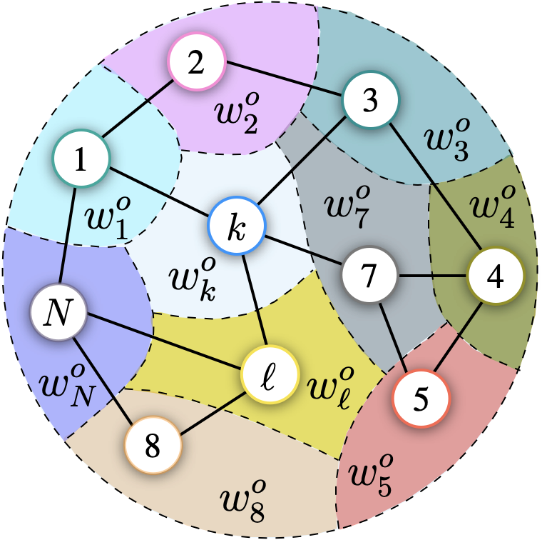
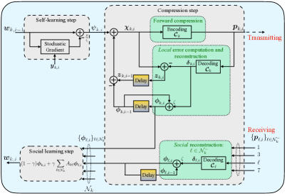
Figure 1: (Left) An illustration of a multitask network [9, 26]. The objective at agent $k$ is to estimate $w^{o}_{k}$ (of dimension $M_{k}\times 1$), the $k$-th subvector of ${\scriptstyle\mathcal{W}}^{o}$ in (2). In this example, the neighborhood set of agent $k$ is given by $\mathcal{N}_{k}=\{1,k,3,\ell,7\}$. (Right) The implementation of the DEF-ATC diffusion approach listed in Alg. 1 at agent $k$. The set $\mathcal{N}_{k}^{-}$ is the neighborhood set of agent $k$, excluding $k$ itself. The compression step consists of three sub-steps: $i)$ the forward compression step where agent $k$ encodes the error-compensated difference $\boldsymbol{\chi}_{k,i}=\boldsymbol{\psi}_{k,i}-\boldsymbol{\phi}_{k,i-1}+\boldsymbol{z}_{k,i-1}$ and sends the resulting vector ${\boldsymbol{p}}_{k,i}$ (sequence of symbols or bits) to its neighbors; $ii)$ the local error computation and reconstruction step where agent $k$ decodes the local vector ${\boldsymbol{p}}_{k,i}$ to obtain $\boldsymbol{\delta}_{k,i}=\boldsymbol{\cal{C}}_{k}(\boldsymbol{\psi}_{k,i}-\boldsymbol{\phi}_{k,i-1}+\boldsymbol{z}_{k,i-1})$, updates the local compression error vector $\boldsymbol{z}_{k,i}$ according to (16) and the local predictor $\boldsymbol{\phi}_{k,i}$ according to (18b); and $iii)$ the (social) reconstruction step where agent $k$ receives the encoded vectors $\{{\boldsymbol{p}}_{\ell,i}\}_{\ell\in\mathcal{N}_{k}^{-}}$ from its neighbors, decodes them to obtain $\{\boldsymbol{\delta}_{\ell,i}\}_{\ell\in\mathcal{N}_{k}^{-}}$, and then updates the predictors $\{\boldsymbol{\phi}_{\ell,i}\}_{\ell\in\mathcal{N}_{k}^{-}}$ according to (15). The resulting vectors $\boldsymbol{\phi}_{k,i}$ and $\{\boldsymbol{\phi}_{\ell,i}\}_{\ell\in\mathcal{N}_{k}^{-}}$ are then used in the social learning step (17). Observe that implementing the compression step requires storing the previous compression error $\boldsymbol{z}_{k,i-1}$ and the previous estimates $\{\boldsymbol{\phi}_{\ell,i-1}\}_{\ell\in\mathcal{N}_{k}}$ by agent $k$.

Input: initializations $\boldsymbol{w}_{k,0}=0$, $\boldsymbol{\phi}_{k,0}=0$, and $\boldsymbol{z}_{k,0}=0$, small step-size $\mu$, damping coefficient $\zeta\in(0,1]$, mixing parameter $\gamma\in(0,1]$, combination matrix $\mathcal{A}$ satisfying (4).

for $i=1,2,\ldots,$ on the $k$-th node do

       Adapt: update $\boldsymbol{w}_{k,i-1}$ according to:

$$\boldsymbol{\psi}_{k,i}=\boldsymbol{w}_{k,i-1}-\frac{\mu}{\zeta}\widehat{\nabla_{w_{k}}J_{k}}(\boldsymbol{w}_{k,i-1})$$ (14)

      

      Compress and broadcast:

       $\bullet$ encode the error compensated difference $\boldsymbol{\psi}_{k,i}-\boldsymbol{\phi}_{k,i-1}+\boldsymbol{z}_{k,i-1}$ using a bounded-distortion compression operator $\boldsymbol{\cal{C}}_{k}(\cdot)$ and broadcast the result $\boldsymbol{p}_{k,i}$ to the neighbors $\mathcal{N}_{k}$

       $\bullet$ upon receiving the compressed messages $\{\boldsymbol{p}_{\ell,i}\}$ from neighbors $\ell\in\mathcal{N}_{k}$, first decode them to obtain $\{\boldsymbol{\delta}_{\ell,i}=\boldsymbol{\cal{C}}_{\ell}(\boldsymbol{\psi}_{\ell,i}-\boldsymbol{\phi}_{\ell,i-1}+\boldsymbol{z}_{\ell,i-1})\}_{\ell\in\mathcal{N}_{k}}$, and then compute $\{\boldsymbol{\phi}_{\ell,i}\}_{\ell\in\mathcal{N}_{k}}$ according to:

$$\boldsymbol{\phi}_{\ell,i}=\boldsymbol{\phi}_{\ell,i-1}+\zeta\boldsymbol{\delta}_{\ell,i},\qquad\ell\in\mathcal{N}_{k}$$ (15)

$\bullet$ update the local compression error:

$${\boldsymbol{z}_{k,i}=(\boldsymbol{\psi}_{k,i}-\boldsymbol{\phi}_{k,i-1}+\boldsymbol{z}_{k,i-1})-\boldsymbol{\delta}_{k,i}}$$ (16)

      

      

      Combine: Update local model according to:

$$\boldsymbol{w}_{k,i}=(1-\gamma)\boldsymbol{\phi}_{k,i}+\gamma\sum_{\ell\in\mathcal{N}_{k}}A_{k\ell}\boldsymbol{\phi}_{\ell,i}$$ (17)

Algorithm 1 DEF-ATC (differential error feedback - adapt then combine) diffusion strategy for solving (2)

For the sake of convenience, we rewrite Algorithm 1 in the following compact form:

$$\boldsymbol{\psi}_{k,i} =\boldsymbol{w}_{k,i-1}-\frac{\mu}{\zeta}\widehat{\nabla_{w_{k}}J_{k}}(\boldsymbol{w}_{k,i-1})$$ (18a)

$$\boldsymbol{\phi}_{k,i} =\boldsymbol{\phi}_{k,i-1}+\zeta\boldsymbol{\cal{C}}_{k}(\boldsymbol{\psi}_{k,i}-\boldsymbol{\phi}_{k,i-1}+\boldsymbol{z}_{k,i-1})$$ (18b)

$$\boldsymbol{w}_{k,i} =(1-\gamma)\boldsymbol{\phi}_{k,i}+\gamma\sum_{\ell\in\mathcal{N}_{k}}A_{k\ell}\boldsymbol{\phi}_{\ell,i}$$ (18c)

where the compression error $\boldsymbol{z}_{k,i}$ is updated according to:

$$\boldsymbol{z}_{k,i}=(\boldsymbol{\psi}_{k,i}-\boldsymbol{\phi}_{k,i-1}+\boldsymbol{z}_{k,i-1})-\boldsymbol{\cal{C}}_{k}(\boldsymbol{\psi}_{k,i}-\boldsymbol{\phi}_{k,i-1}+\boldsymbol{z}_{k,i-1}).$$ (19)

Observe that, in the absence of compression (i.e., when the operator $\boldsymbol{\cal{C}}_{k}(\cdot)$ in (18b) and (19) is replaced by the identity operator and the parameters $\zeta$ and $\gamma$ in (18b) and (18c), respectively, are set to 1) we recover the diffusion ATC approach (3). Therefore, Algorithm 1 can be seen as a communication-efficient variant of the Adapt-Then-Combine (ATC) approach. To mitigate the negative impact of compression, the DEF-ATC approach uses differential quantization and error-feedback in step (18b). Differential quantization consists of compressing differences of the form $\boldsymbol{\psi}_{k,i}-\boldsymbol{\phi}_{k,i-1}$ and transmitting them, instead of communicating compressed versions of the estimates $\boldsymbol{\psi}_{k,i}$. Error feedback, on the other hand, consists of locally storing the compression error $\boldsymbol{z}_{k,i}$ (i.e., the difference between the input and output of the compression operator), and incorporating it back into the next iteration. In Remark 1 further ahead, we explain the role of the compression error $\boldsymbol{z}_{k,i}$ and how its introduction helps mitigate the accumulation of errors over time.

IV Mean-square-error and bit rate stability analysis

IV-A Modeling assumptions

In this section, we analyze strategy (18) with a matrix $\mathcal{A}$ satisfying (4) by examining the average squared distance between $\boldsymbol{w}_{k,i}$ and $w^{o}_{k}$, namely, $\mathbb{E}\|w^{o}_{k}-\boldsymbol{w}_{k,i}\|^{2}$, under the following assumptions on the risks $\{J_{k}(\cdot)\}$, the gradient noise processes $\{\boldsymbol{s}_{k,i}(\cdot)\}$ defined by [6]:

$$\boldsymbol{s}_{k,i}(w)\triangleq\nabla_{w_{k}}J_{k}(w)-\widehat{\nabla_{w_{k}}J_{k}}(w),$$ (20)

and the compression operators $\{\boldsymbol{\cal{C}}_{k}(\cdot)\}$.

Assumption 1.

(Conditions on individual and aggregate risks). The individual risks $J_{k}(w_{k})$ are assumed to be twice differentiable and convex such that:

$$\lambda_{k,\min}I_{M_{k}}\leq\nabla^{2}_{w_{k}}J_{k}(w_{k})\leq\lambda_{k,\max}I_{M_{k}},$$ (21)

where $\lambda_{k,\min}\geq 0$ for $k=1,\ldots,K$. It is further assumed that, for any $\{w_{k}\in\mathbb{R}^{M_{k}}\}$, the individual risks satisfy:

$$0<\lambda_{\min}I_{P}\leq\mathcal{U}^{\top}\emph{\text{diag}}\left\{\nabla^{2}_{w_{k}}J_{k}(w_{k})\right\}_{k=1}^{K}\mathcal{U}\leq\lambda_{\max}I_{P},$$ (22)

for some positive parameters $\lambda_{\min}\leq\lambda_{\max}$. ∎

As explained in [40], condition (22) ensures that problem (2) has a unique minimizer ${\scriptstyle\mathcal{W}}^{o}$.

Assumption 2.

(Conditions on gradient noise). The gradient noise process defined in (20) satisfies for $k=1,\ldots,K$:

$$\mathbb{E}\left[\boldsymbol{s}_{k,i}(\boldsymbol{w}_{k,i-1})|\{{\boldsymbol{\phi}_{\ell,i-1},\boldsymbol{z}_{\ell,i-1}}\}_{\ell=1}^{K}\right] =0,$$ (23)

$$\mathbb{E}\left[\|\boldsymbol{s}_{k,i}(\boldsymbol{w}_{k,i-1})\|^{2}|\{{\boldsymbol{\phi}_{\ell,i-1},\boldsymbol{z}_{\ell,i-1}}\}_{\ell=1}^{K}\right] \leq\beta^{2}_{s,k}\|{w^{o}_{k}-\boldsymbol{w}_{k,i-1}}\|^{2}+\sigma^{2}_{s,k},$$ (24)

for some $\beta^{2}_{s,k}\geq 0$ and $\sigma^{2}_{s,k}\geq 0$. ∎

As explained in [6, 7, 8], these conditions are satisfied by many risk functions of interest in learning and adaptation such as quadratic and regularized logistic costs. Condition (23) states that the gradient vector approximation should be unbiased conditioned on the iterates generated at the previous time instant. Condition (24) states that the second-order moment of the gradient noise should get smaller for better estimates, since it is bounded by the squared norm of the iterate.

Assumption 3.

(Conditions on compression operators). In step (18b) of the DEF-ATC strategy, each agent $k$ at time $i$ applies to the error compensated difference $\boldsymbol{\chi}_{k,i}=\boldsymbol{\psi}_{k,i}-\boldsymbol{\phi}_{k,i-1}+\boldsymbol{z}_{k,i-1}$ a bounded-distortion compression operator $\boldsymbol{\cal{C}}_{k}(\cdot)$ (see Definition 2) with compression noise parameters $\beta^{2}_{c,k}$ and $\sigma^{2}_{c,k}$. It is assumed that given the past history, the randomized compression mechanism depends only on the quantizer input $\boldsymbol{\chi}_{k,i}$. Consequently, from (7), we get:

$$\mathbb{E}\left[\|\boldsymbol{\chi}_{k,i}-\boldsymbol{\cal{C}}_{k}(\boldsymbol{\chi}_{k,i})\|^{2}|\boldsymbol{h}_{i}\right] =\mathbb{E}\left[\|\boldsymbol{\chi}_{k,i}-\boldsymbol{\cal{C}}_{k}(\boldsymbol{\chi}_{k,i})\|^{2}|\boldsymbol{\chi}_{k,i}\right]\leq\beta^{2}_{c,k}\|\boldsymbol{\chi}_{k,i}\|^{2}+\sigma^{2}_{c,k},$$ (25)

where $\boldsymbol{h}_{i}$ is the vector collecting all iterates generated by (18) before the quantizer is applied to $\boldsymbol{\chi}_{k,i}$, namely, $\Big{\{}\{\boldsymbol{\phi}_{\ell,j}\}_{j=1}^{i-1},\{\boldsymbol{\psi}_{\ell,j}\}_{j=1}^{i},\{\boldsymbol{z}_{\ell,j}\}_{j=1}^{i-1}\Big{\}}_{\ell=1}^{K}$ . ∎

IV-B Network error vector recursion

In the following, we derive a useful recursion that allows to examine the time-evolution across the network of the error dynamics relative to the reference vector ${\scriptstyle\mathcal{W}}^{o}=\text{col}\{w^{o}_{k}\}_{k=1}^{K}$ defined in (2). Let $\widetilde{\boldsymbol{w}}_{k,i}=w^{o}_{k}-\boldsymbol{w}_{k,i}$, $\widetilde{\boldsymbol{\psi}}_{k,i}=w^{o}_{k}-\boldsymbol{\psi}_{k,i}$, and $\widetilde{\boldsymbol{\phi}}_{k,i}=w^{o}_{k}-\boldsymbol{\phi}_{k,i}$. Using (20) and the mean-value theorem [47, pp. 24], [6, Appendix D], we can express the stochastic gradient vector appearing in (18a) as follows:

$$\widehat{\nabla_{w_{k}}J_{k}}(\boldsymbol{w}_{k,i-1})=-\boldsymbol{H}_{k,i-1}\widetilde{\boldsymbol{w}}_{k,i-1}+b_{k}-\boldsymbol{s}_{k,i}(\boldsymbol{w}_{k,i-1}){,}$$ (26)

where $\boldsymbol{H}_{k,i-1}\triangleq\int_{0}^{1}\nabla^{2}_{w_{k}}J_{k}(w^{o}_{k}-t\widetilde{\boldsymbol{w}}_{k,i-1})dt$ and $b_{k}\triangleq\nabla_{w_{k}}J_{k}(w^{o}_{k})$. By subtracting $w^{o}_{k}$ from both sides of (18a), by using (26), and by introducing the following network quantities:

$$b \triangleq\text{col}\left\{b_{1},\ldots,b_{K}\right\},$$ (27)

$$\boldsymbol{s}_{i} \triangleq\text{col}\left\{\boldsymbol{s}_{1,i}(\boldsymbol{w}_{1,i-1}),\ldots,\boldsymbol{s}_{K,i}(\boldsymbol{w}_{K,i-1})\right\},$$ (28)

$$\boldsymbol{\cal{H}}_{i-1} \triangleq\text{diag}\left\{\boldsymbol{H}_{1,i-1},\ldots,\boldsymbol{H}_{K,i-1}\right\},$$ (29)

$$\widetilde{\boldsymbol{{\scriptstyle\mathcal{W}}}}_{i-1} \triangleq\text{col}\{\widetilde{\boldsymbol{w}}_{1,i-1},\ldots,\widetilde{\boldsymbol{w}}_{K,i-1}\},$$ (30)

we can show that the network error vector $\widetilde{\boldsymbol{\psi}}_{i}=\text{col}\{\widetilde{\boldsymbol{\psi}}_{k,i}\}_{k=1}^{K}$ evolves according to:

$$\widetilde{\boldsymbol{\psi}}_{i}=\left(I_{M}-\frac{\mu}{\zeta}\boldsymbol{\cal{H}}_{i-1}\right)\widetilde{\boldsymbol{{\scriptstyle\mathcal{W}}}}_{i-1}-\frac{\mu}{\zeta}\boldsymbol{s}_{i}+\frac{\mu}{\zeta}b.$$ (31)

By subtracting $w^{o}_{k}$ from both sides of (18c), by replacing $w^{o}_{k}$ by $(1-\gamma)w^{o}_{k}+\gamma w^{o}_{k}$, and by using $w^{o}_{k}=\sum_{\ell\in\mathcal{N}_{k}}A_{k\ell}w^{o}_{\ell}$ [40, Sec. III-B], we obtain:

$$\begin{split}\widetilde{\boldsymbol{w}}_{k,i}&=(1-\gamma)\widetilde{\boldsymbol{\phi}}_{k,i}+\gamma\sum_{\ell\in\mathcal{N}_{k}}A_{k\ell}\widetilde{\boldsymbol{\phi}}_{\ell,i}.\end{split}$$ (32)

From (32), we find that the network error vector $\widetilde{\boldsymbol{{\scriptstyle\mathcal{W}}}}_{i-1}$ in (30) evolves according to:

$$\widetilde{\boldsymbol{{\scriptstyle\mathcal{W}}}}_{i-1}=(1-\gamma)\widetilde{\boldsymbol{\phi}}_{i-1}+\gamma\mathcal{A}\widetilde{\boldsymbol{\phi}}_{i-1}=\mathcal{A}^{\prime}\widetilde{\boldsymbol{\phi}}_{i-1},$$ (33)

where

$$\widetilde{\boldsymbol{\phi}}_{i} \triangleq\text{col}\{\widetilde{\boldsymbol{\phi}}_{1,i},\ldots,\widetilde{\boldsymbol{\phi}}_{K,i}\}{,}$$ (34)

$$\mathcal{A}^{\prime} \triangleq(1-\gamma)I_{M}+\gamma\mathcal{A}{.}$$ (35)

By subtracting $w^{o}_{k}$ from both sides of (18b) and by adding and subtracting $w^{o}_{k}$ to the difference $\boldsymbol{\psi}_{k,i}-\boldsymbol{\phi}_{k,i-1}$, we can write:

$$\widetilde{\boldsymbol{\phi}}_{k,i}=\widetilde{\boldsymbol{\phi}}_{k,i-1}-\zeta\boldsymbol{\cal{C}}_{k}(\widetilde{\boldsymbol{\phi}}_{k,i-1}-\widetilde{\boldsymbol{\psi}}_{k,i}+\boldsymbol{z}_{k,i-1}).$$ (36)

Now, by adding and subtracting $\zeta(\widetilde{\boldsymbol{\phi}}_{k,i-1}-\widetilde{\boldsymbol{\psi}}_{k,i}+\boldsymbol{z}_{k,i-1})$ to the RHS of the above equation, we obtain:

$$\widetilde{\boldsymbol{\phi}}_{k,i}=(1-\zeta)\widetilde{\boldsymbol{\phi}}_{k,i-1}+\zeta\widetilde{\boldsymbol{\psi}}_{k,i}+\zeta(\boldsymbol{z}_{k,i}-\boldsymbol{z}_{k,i-1}),$$ (37)

in terms of the compression error vector $\boldsymbol{z}_{k,i}$ defined in (19). By combining (31), (33), and (37), we conclude that the network error vector $\widetilde{\boldsymbol{\phi}}_{i}$ in (34) evolves according to the following dynamics:

$$\widetilde{\boldsymbol{\phi}}_{i}=\boldsymbol{\cal{B}}_{i-1}\widetilde{\boldsymbol{\phi}}_{i-1}-\mu\boldsymbol{s}_{i}+\mu b+\left(\boldsymbol{z}_{i}-\boldsymbol{z}_{i-1}\right),$$ (38)

where

$$\boldsymbol{\cal{B}}_{i-1} \triangleq(1-\zeta)I_{M}+\zeta\left(I_{M}-\frac{\mu}{\zeta}\boldsymbol{\cal{H}}_{i-1}\right)\mathcal{A}^{\prime},$$ (39)

$$\boldsymbol{z}_{i} \triangleq\zeta\text{col}\left\{\boldsymbol{z}_{k,i}\right\}_{k=1}^{K}.$$ (40)

Remark 1 (Temporal filtering of the compression error): A direct consequence of feeding back the error in the compression step (18b) is to subtract the compression error from previous instants in recursion (38), thereby allowing for a correction mechanism. This correction helps mitigate the accumulation of errors over time, leading to improved network performance. $\blacksquare$

As the presentation will reveal, the study of the network behavior in the presence of error feedback is a challenging task since, in addition to analyzing the dynamics of the network error vector $\widetilde{\boldsymbol{\phi}}_{i}$, we need to examine how the compression error (40), which is fed back into the network through the compression step (18b), affects its behavior. When all is said and done, the results will help clarify the effect of network topology, step-size $\mu$, damping coefficient $\zeta$, mixing parameter $\gamma$, gradient (through $\{\beta^{2}_{s,k},\sigma^{2}_{s,k}\}$) and compression (through $\{\beta^{2}_{c,k},\sigma^{2}_{c,k}\}$) noise processes on the network mean-square-error stability and performance, and will provide insights into the design of effective compression operators for decentralized learning.

IV-C Mean-square-error stability

The mean-square-error analysis will be carried out by first establishing the boundedness of $\limsup_{i\rightarrow\infty}\mathbb{E}\|\widetilde{\boldsymbol{\phi}}_{i}-\boldsymbol{z}_{i}\|^{2}$, and then using relation (33) and Holder’s and Jensen’s inequalities to deduce boundedness of $\limsup_{i\rightarrow\infty}\mathbb{E}\|\widetilde{\boldsymbol{{\scriptstyle\mathcal{W}}}}_{i}\|^{2}$. Therefore, in the following, we first study the stability of the network error vector $\widetilde{\boldsymbol{\phi}}_{i}^{z}$ defined as $\widetilde{\boldsymbol{\phi}}_{i}^{z}\triangleq\widetilde{\boldsymbol{\phi}}_{i}-\boldsymbol{z}_{i}$ and evolving according to:

$$\boxed{\widetilde{\boldsymbol{\phi}}_{i}^{z}=\boldsymbol{\cal{B}}_{i-1}\widetilde{\boldsymbol{\phi}}^{z}_{i-1}-\mu\boldsymbol{s}_{i}+\mu b-(I_{M}-\boldsymbol{\cal{B}}_{i-1})\boldsymbol{z}_{i-1}}$$ (42)

The above identity can be found by adding and subtracting the term $\boldsymbol{\cal{B}}_{i-1}\boldsymbol{z}_{i-1}$ to the RHS of (38). We analyze the stability of recursion (42) by first transforming it into a more convenient form (shown later in (65) and (66)) using the Jordan canonical decomposition [48] of the matrix $\mathcal{A}^{\prime}$ defined in (35). To exploit the eigen-structure of $\mathcal{A}^{\prime}$, we first recall that a matrix $\mathcal{A}$ satisfying the conditions in (4) (for a full-column rank semi-unitary matrix $\mathcal{U}$) has a Jordan decomposition of the form $\mathcal{A}=\mathcal{V}_{\epsilon}\Lambda_{\epsilon}\mathcal{V}_{\epsilon}^{-1}$ with [40, Lemma 2]:

$$\mathcal{V}_{\epsilon}=\left[\begin{array}[]{c|c}\mathcal{U}&\mathcal{V}_{R,\epsilon}\end{array}\right],~{}\Lambda_{\epsilon}=\left[\begin{array}[]{c|c}I_{P}&0\\ \hline\cr 0&\mathcal{J}_{\epsilon}\end{array}\right],~{}\mathcal{V}_{\epsilon}^{-1}=\left[\begin{array}[]{c}\mathcal{U}^{\top}\\ \hline\cr\mathcal{V}_{L,\epsilon}^{\top}\end{array}\right],$$ (43)

where $\mathcal{J}_{\epsilon}$ is a Jordan matrix with eigenvalues (which may be complex but have magnitude less than one) on the diagonal and $\epsilon>0$ on the super-diagonal [40, Lemma 2],[6, pp. 510]. The parameter $\epsilon$ is chosen small enough to ensure $\rho(\mathcal{J}_{\epsilon})+\epsilon\in(0,1)$ [40]. Consequently, the matrix $\mathcal{A}^{\prime}$ in (35) has a Jordan decomposition of the form $\mathcal{A}^{\prime}=\mathcal{V}_{\epsilon}\Lambda^{\prime}_{\epsilon}\mathcal{V}_{\epsilon}^{-1}$ where:

$$\Lambda^{\prime}_{\epsilon}=\left[\begin{array}[]{c|c}I_{P}&0\\ \hline\cr 0&\mathcal{J}^{\prime}_{\epsilon}\end{array}\right],\quad{\text{with }}\mathcal{J}^{\prime}_{\epsilon}\triangleq(1-\gamma)I_{M-P}+\gamma\mathcal{J}_{\epsilon}.$$ (44)

By multiplying both sides of (42) from the left by $\mathcal{V}_{\epsilon}^{-1}$ in (43), we obtain the transformed iterates and variables:

$$\mathcal{V}_{\epsilon}^{-1}\widetilde{\boldsymbol{\phi}}_{i}^{z} =\left[\begin{array}[]{c}\mathcal{U}^{\top}\widetilde{\boldsymbol{\phi}}^{z}_{i}\\ \mathcal{V}_{L,\epsilon}^{\top}\widetilde{\boldsymbol{\phi}}^{z}_{i}\end{array}\right]\triangleq\left[\begin{array}[]{c}\overline{\boldsymbol{\phi}}^{z}_{i}\\ \widecheck{\boldsymbol{\phi}}^{z}_{i}\end{array}\right],$$ (49)

$$\mathcal{V}_{\epsilon}^{-1}\boldsymbol{s}_{i} =\left[\begin{array}[]{c}\mathcal{U}^{\top}\boldsymbol{s}_{i}\\ \mathcal{V}_{L,\epsilon}^{\top}\boldsymbol{s}_{i}\end{array}\right]\triangleq\left[\begin{array}[]{c}\overline{\boldsymbol{s}}_{i}\\ \widecheck{\boldsymbol{s}}_{i}\end{array}\right],$$ (54)

$$\mathcal{V}_{\epsilon}^{-1}b =\left[\begin{array}[]{c}\mathcal{U}^{\top}b\\ \mathcal{V}_{L,\epsilon}^{\top}b\end{array}\right]\triangleq\left[\begin{array}[]{c}0\\ \widecheck{b}\end{array}\right],$$ (59)

$$\mathcal{V}_{\epsilon}^{-1}\boldsymbol{z}_{i-1} =\left[\begin{array}[]{c}\mathcal{U}^{\top}\boldsymbol{z}_{i-1}\\ \mathcal{V}_{L,\epsilon}^{\top}\boldsymbol{z}_{i-1}\end{array}\right]\triangleq\left[\begin{array}[]{c}\overline{\boldsymbol{z}}_{i-1}\\ \widecheck{\boldsymbol{z}}_{i-1}\end{array}\right],$$ (64)

where in (59) we used the fact that $\mathcal{U}^{\top}b=0$ as shown in [40, Sec. III-B]. In particular, the transformed components $\overline{\boldsymbol{\phi}}^{z}_{i}$ and ${\widecheck{\boldsymbol{\phi}}}^{z}_{i}$ evolve according to the recursions:

$$\overline{\boldsymbol{\phi}}^{z}_{i} =(I_{P}-\mu\boldsymbol{\cal{D}}_{11,i-1})\overline{\boldsymbol{\phi}}^{z}_{i-1}-\mu\boldsymbol{\cal{D}}_{12,i-1}\widecheck{\boldsymbol{\phi}}^{z}_{i-1}-\mu\overline{\boldsymbol{s}}_{i}-\mu\boldsymbol{\cal{D}}_{11,i-1}\overline{\boldsymbol{z}}_{i-1}-\mu\boldsymbol{\cal{D}}_{12,i-1}\widecheck{\boldsymbol{z}}_{i-1}$$ (65)

$${\widecheck{\boldsymbol{\phi}}}^{z}_{i} =(\mathcal{J}^{\prime\prime}_{\epsilon}-\mu\boldsymbol{\cal{D}}_{22,i-1})\widecheck{\boldsymbol{\phi}}^{z}_{i-1}-\mu\boldsymbol{\cal{D}}_{21,i-1}\overline{\boldsymbol{\phi}}^{z}_{i-1}+\mu\widecheck{b}-\mu\widecheck{\boldsymbol{s}}_{i}-\mu\boldsymbol{\cal{D}}_{21,i-1}\overline{\boldsymbol{z}}_{i-1}-\left(\zeta(I-\mathcal{J}_{\epsilon}^{\prime})+\mu\boldsymbol{\cal{D}}_{22,i-1}\right)\widecheck{\boldsymbol{z}}_{i-1}$$ (66)

where

$$\boldsymbol{\cal{D}}_{11,i-1} \triangleq\mathcal{U}^{\top}\boldsymbol{\cal{H}}_{i-1}\mathcal{U},$$ (67)

$$\boldsymbol{\cal{D}}_{12,i-1} \triangleq\mathcal{U}^{\top}\boldsymbol{\cal{H}}_{i-1}\mathcal{V}_{R,\epsilon}\mathcal{J}_{\epsilon}^{\prime},$$ (68)

$$\boldsymbol{\cal{D}}_{21,i-1} \triangleq\mathcal{V}_{L,\epsilon}^{\top}\boldsymbol{\cal{H}}_{i-1}\mathcal{U},$$ (69)

$$\boldsymbol{\cal{D}}_{22,i-1} \triangleq\mathcal{V}_{L,\epsilon}^{\top}\boldsymbol{\cal{H}}_{i-1}\mathcal{V}_{R,\epsilon}\mathcal{J}_{\epsilon}^{\prime},$$ (70)

$$\mathcal{J}^{\prime\prime}_{\epsilon} \triangleq(1-\zeta)I_{M-P}+\zeta\mathcal{J}^{\prime}_{\epsilon}.$$ (71)

Theorem 1.

(Mean-square-error stability). Consider a network of $K$ agents running the DEF-ATC diffusion approach (listed in Algorithm 1) to solve problem (2) under Assumptions 1, 2, and 3, with a matrix $\mathcal{A}$ satisfying (4). In the absence of the relative compression noise term (i.e., $\beta^{2}_{c,k}=0$, $\forall k$), let the damping and mixing parameters be such that $\zeta=\gamma=1$. In the presence of the relative compression noise (i.e., at least one $\beta^{2}_{c,k}$ is positive for some agent $k$), let $\zeta\in(0,1]$ and $\gamma\in(0,1]$ be such that the two following conditions are satisfied:

$${0<\gamma\zeta<\frac{1-(\rho(\mathcal{J}_{\epsilon})+\epsilon)}{4v_{1}^{2}v_{2}^{2}\beta^{2}_{c,\max}(\rho(I-\mathcal{J}_{\epsilon})+\epsilon)^{2}},}$$ (72)

and

$$\begin{split}{\gamma\zeta\frac{(\rho(I-\mathcal{J}_{\epsilon})+\epsilon)^{2}}{1-(\rho(\mathcal{J}_{\epsilon})+\epsilon)}+\zeta^{2}\beta_{c,\max}^{2}v_{1}^{2}v_{2}^{2}\left(1+\left((1+\gamma)-\gamma(\rho(\mathcal{J}_{\epsilon})+\epsilon)\right)^{2}\right)<\frac{1}{2},}\end{split}$$ (73)

where $v_{1}=\|\mathcal{V}_{\epsilon}^{-1}\|$, $v_{2}=\|\mathcal{V}_{\epsilon}\|$, and ${\beta}_{c,\max}^{2}\triangleq\max_{1\leq k\leq K}\{{\beta}^{2}_{c,k}\}$. Then, for sufficiently small step-size $\mu$, the network is mean-square-error stable, and it holds that:

$$\limsup_{i\rightarrow\infty}\mathbb{E}\|\widetilde{\boldsymbol{\phi}}^{z}_{i}\|^{2}=\kappa\mu+\overline{\sigma}^{2}_{c}O(1),$$ (74)

where $\overline{\sigma}^{2}_{c}=\sum_{k=1}^{K}{\sigma}^{2}_{c,k}$. The constant $\kappa$ is positive, independent of the step-size $\mu$ and the compression noise terms $\{\beta^{2}_{c,k},\sigma^{2}_{c,k}\}$, and is given by $\kappa=v_{1}^{2}v_{2}^{2}\frac{\overline{\sigma}^{2}_{s}}{\sigma_{11}}$ with $\overline{\sigma}^{2}_{s}=\sum_{k=1}^{K}\sigma_{s,k}^{2}$, and $\sigma_{11}$ is some positive constant resulting from the derivation of inequality (90) in Appendix B. Moreover, by choosing compression schemes with $\sigma^{2}_{c,k}\propto\mu^{1+\varepsilon}$ (where the symbol $\propto$ hides a proportionality constant independent of $\mu$) and $\varepsilon\in(0,1]$, we obtain:

$${\limsup_{i\rightarrow\infty}\mathbb{E}\|\widetilde{\boldsymbol{\phi}}^{z}_{i}\|^{2}=\kappa\mu+O(\mu^{1+{\varepsilon}}).}$$ (75)

It then holds that:

$$\limsup_{i\rightarrow\infty}\mathbb{E}\|\widetilde{\boldsymbol{{\scriptstyle\mathcal{W}}}}_{i}\|^{2}=\kappa\mu+O(\mu^{1+\frac{\varepsilon}{2}}),$$ (76)

from which we conclude that:

$${\lim_{\mu\rightarrow 0}\limsup_{i\rightarrow\infty}\frac{1}{\mu}\mathbb{E}\|w^{o}_{k}-\boldsymbol{w}_{k,i}\|^{2}}=\kappa,$$ (77)

for $k=1,\ldots,K$.

Proof.

See Appendix B. ∎

While expressions (74)–(77) in Theorem 1 reveal the influence of the step-size $\mu$, the compression noise (captured by $\{\overline{\sigma}^{2}_{c},\beta^{2}_{c,\max}\}$), and the gradient noise (captured by $\overline{\sigma}^{2}_{s}$) on the steady-state mean-square error, expressions (72) and (73) reveal the influence of the relative compression noise term (captured by $\beta^{2}_{c,\max}$) on the network stability, and how this influence can be mitigated by properly choosing the damping coefficient $\zeta$ and the mixing parameter $\gamma$. One main conclusion stemming from Theorem 1 (expression (74)) is that the mean-square-error contains two terms. The first term is $\kappa\mu$ where $\kappa$ is a constant independent of the compression noise $\{\beta^{2}_{c,k},\sigma^{2}_{c,k}\}$, but depends on the gradient noise $\{\sigma^{2}_{s,k}\}$. This term, which we refer to as the gradient noise term, is classically encountered in the uncompressed case [40]. The second factor is an $O(1)$ term that is proportional to the quantizers’ absolute noise components $\{\sigma^{2}_{c,k}\}$. Interestingly, by choosing compression schemes with $\sigma^{2}_{c,k}\propto\mu^{1+\varepsilon}$ and $\varepsilon\in(0,1]$, for sufficiently small step-sizes $\mu$ we obtain $\limsup_{i\rightarrow\infty}\mathbb{E}\|w^{o}_{k}-\boldsymbol{w}_{k,i}\|^{2}\approx\kappa\mu$. This result is reassuring since it implies that the impact of the compression noise can be minimized to the point where it only affects higher-order terms of the step-size. Consequently, the primary noise influencing the learning process will be the gradient noise, which is consistent with the classical results observed in the uncompressed case studied in [40].

While result (77) is appealing, it is not sufficient to characterize the DEF-ATC diffusion approach. To fully characterize a decentralized strategy endowed with a compression mechanism, it is essential to consider the learning-communication tradeoff. In other words, we need to assess also how the design choice $\sigma^{2}_{c,k}\propto\mu^{1+\varepsilon}$ impacts the amount of communication resources (e.g., quantization bits). For instance, consider the probabilistic uniform quantizer from Table II. For this scheme, setting $\sigma^{2}_{c,k}\propto\mu^{1+\varepsilon}$ is equivalent to requiring the quantization step $\Delta$ to be proportional to $\mu^{\frac{1+\varepsilon}{2}}$. Thus, while small values of $\sigma^{2}_{c,k}$ imply small compression errors in view of (7), they might in principle require large bit rates. Moreover, as $\mu\rightarrow 0$, the quantization step $\Delta$ becomes very small, potentially leading to an unbounded bit rate increase. It becomes therefore important to find a quantization scheme that achieves the same performance as the uncompressed case, i.e., $\limsup_{i\rightarrow\infty}\mathbb{E}\|w^{o}_{k}-\boldsymbol{w}_{k,i}\|^{2}\approx\kappa\mu$, while guaranteeing a finite bit rate as $\mu\rightarrow 0$. In the next theorem, we show that the DEF-ATC diffusion approach equipped with the variable-rate coding scheme from [25], [26, Sec. II] achieves both objectives.

IV-D Bit rate stability

We first assume that the top-$c_{k}$ quantizer in Definition 4 (with a subscript $k$ added to $c$ to highlight the fact that the compression characteristics can vary across agents) is used at each iteration $i$ and agent $k$. We then recall that the quantizer input is given by the error compensated difference $\boldsymbol{\chi}_{k,i}=\boldsymbol{\psi}_{k,i}-\boldsymbol{\phi}_{k,i-1}+\boldsymbol{z}_{k,i-1}$, and assume that the probabilistic ANQ scheme (Table II, row $3$) is employed at the output of the top-$c_{k}$ sparsifier. Consequently, from (9), the bit rate at agent $k$ and iteration $i$ is given by:

$${{r}_{k,i}}=\log_{2}(3)\sum_{j\in\mathcal{I}_{c_{k,i}}}\Big{(}1+\mathbb{E}\Big{[}\left\lceil\log_{2}(|\boldsymbol{n}([\boldsymbol{\chi}_{k,i}]_{j})|+1)\right\rceil\Big{]}\Big{)}+(M_{k}-c_{k})\log_{2}(3),$$ (78)

where $[\boldsymbol{\chi}_{k,i}]_{j}$ denotes the $j$-th entry of $\boldsymbol{\chi}_{k,i}$, $\mathcal{I}_{c_{k,i}}$ is the set containing the indices of the $c_{k}$ largest-magnitude components of $\boldsymbol{\chi}_{k,i}$, and $(M_{k}-c_{k})\log_{2}(3)$ is the number of bits required to encode the $M_{k}-c_{k}$ zero components at the output of the top-$c_{k}$ sparsifier.

Theorem 2.

(Bit rate stability). Assume that each agent $k$ employs the top-$c_{k}$ quantizer (see Definition 4) with the probabilistic ANQ scheme. Assume further that the design parameters of the compression operators are chosen such that:

$$\omega_{k}=t,\qquad\eta_{k}\propto\mu^{\frac{1+\varepsilon}{2}},$$ (79)

where $t$ is a constant independent of $\mu$ and $0<\varepsilon\leq 1$. First, under conditions (79), we have:

$$\sigma^{2}_{c,k}\propto\mu^{1+\varepsilon}.$$ (80)

Second, in the steady state, the average number of bits at agent $k$ stays bounded as $\mu\rightarrow 0$, namely,

$$\limsup_{i\rightarrow\infty}\,{r}_{k,i}=O(1).$$ (81)

Proof.

See Appendix C. ∎

The bit rate stability result (81) can be explained by considering again the uniform quantization rule (Table II, row $2$) which, as explained previously, requires setting $\Delta\propto\mu^{\frac{1+\varepsilon}{2}}$ in order to guarantee that $\sigma^{2}_{c,k}\propto\mu^{1+\varepsilon}$. The result (159) reveals that the input to the compression operators of the DEF-ATC strategy in (18b), namely, the error compensated difference $\boldsymbol{\chi}_{k,i}=\boldsymbol{\psi}_{k,i}-\boldsymbol{\phi}_{k,i-1}+\boldsymbol{z}_{k,i-1}$, under (80) is on the order of $\mu^{\frac{1+\varepsilon}{2}}$ at steady-state. This means that as $\mu\rightarrow 0$, the quantizer resolution $\Delta\propto\mu^{\frac{1+\varepsilon}{2}}$ decreases, but in proportion to the effective range of the quantizers’ inputs. Theorem 2 reveals the adaptability of the variable-rate scheme, ensuring that even as the quantization becomes increasingly precise (as $\mu\rightarrow 0$), the DEF-ATC strategy can still maintain a finite expected bit rate, which is crucial for efficient data transmission.

V Simulation results

In this section, we first illustrate the theoretical results of Theorems 1 and 2. Then, we illustrate the benefit of the top-$c$ quantizer over other quantizers, particularly those that quantize a vector element-wise, without prioritizing the $c$ most important components. In the third part, we compare DEF-ATC to state-of-the-art baselines in various scenarios, including those beyond the small step-size regime. The first three parts focus on solving single-task optimization problems of the form (1). The last part illustrates the performance of the DEF-ATC approach when used to solve multitask estimation problems with overlapping parameter vectors.

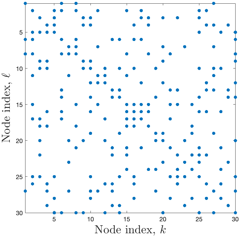
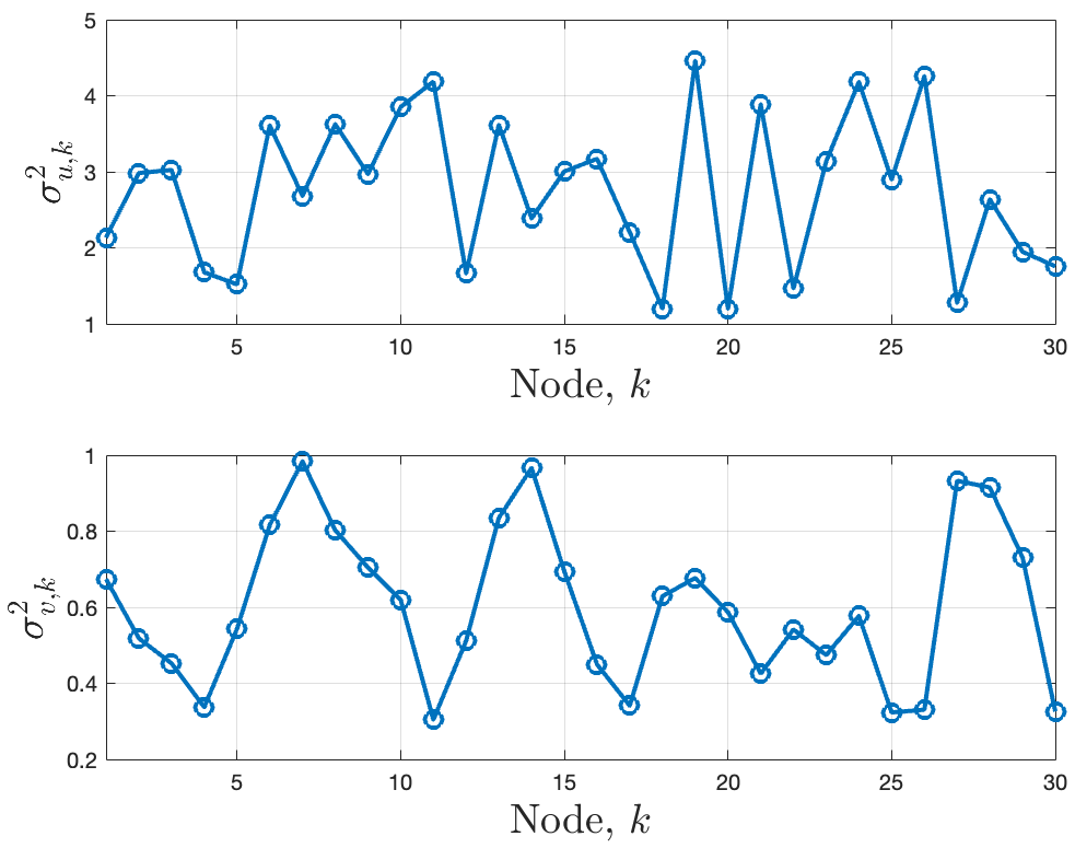
Figure 2: Experimental setup. (Left) Communication link matrix. (Right) Regression and noise variances.

We consider a network of $K=30$ nodes with the communication link matrix shown in Fig. 2 (left), where the $(k,\ell)$-th entry is equal to $1$ if there is a link between $k$ and $\ell$ and is 0 otherwise. Each agent is subjected to streaming data $\{\boldsymbol{d}_{k}(i),\boldsymbol{u}_{k,i}\}$ assumed to satisfy a linear regression model of the form $\boldsymbol{d}_{k}(i)=\boldsymbol{u}_{k,i}^{\top}w^{\star}_{k}+\boldsymbol{v}_{k}(i)$ for some ${{M_{c}}}\times 1$ vector $w^{\star}_{k}$ with $\boldsymbol{v}_{k}(i)$ denoting a zero-mean measurement noise and ${{M_{c}}}=10$. A mean-square-error risk of the form $J_{k}(w_{k})=\mathbb{E}|\boldsymbol{d}_{k}(i)-\boldsymbol{u}_{k,i}^{\top}w_{k}|^{2}$ is associated with each agent $k$. The processes $\{\boldsymbol{u}_{k,i},\boldsymbol{v}_{k}(i)\}$ are assumed to be zero-mean Gaussian with: $i)$ $\mathbb{E}\boldsymbol{u}_{k,i}\boldsymbol{u}_{\ell,i}^{\top}=R_{u,k}=\sigma^{2}_{u,k}I_{{M_{c}}}$ if $k=\ell$ and $0$ otherwise; $ii)$ $\mathbb{E}\boldsymbol{v}_{k}(i)\boldsymbol{v}_{\ell}(i)=\sigma^{2}_{v,k}$ if $k=\ell$ and $0$ otherwise; and $iii)$ $\boldsymbol{u}_{k,i}$ and $\boldsymbol{v}_{k}(i)$ are independent of each other. The variances $\sigma^{2}_{u,k}$ and $\sigma^{2}_{v,k}$ are shown in Fig. 2 (right). Throughout Sec. V, we assume that all agents employ the same compression rule, i.e., $\boldsymbol{\cal{C}}_{k}=\boldsymbol{\cal{C}}$ $\forall k$. We use the terminology “top-$c$ quantizer-name” to refer to the top-$c$ quantizer of Definition 4 where, as compression scheme $\boldsymbol{\cal{Q}}$, we use quantizer-name. For instance, “top-$4$ probabilistic ANQ” is the quantizer obtained by applying the probabilistic ANQ scheme at the output of the top-$4$ sparsifier.

V-A Illustrating the theoretical findings

In this section and the following Secs. V-B and V-C, we assume that agents have a common model parameter $w^{\star}_{k}=w^{o}$ $\forall k$. The model $w^{o}$ is generated by normalizing to unit norm a randomly generated Gaussian vector, with zero mean and unit variance. To promote consensus (i.e., to solve problem (1) or, equivalently, (2) with $\mathcal{U}=\frac{1}{\sqrt{K}}(\mathds{1}_{K}\otimes I_{{M_{c}}})$), we run Alg. 1 using a combination matrix of the form $\mathcal{A}=A\otimes I_{{M_{c}}}$, where $A$ is generated according to the Metropolis rule [6, Chap. 8].

In Fig. 3 (left), we report the network mean-square-deviation (MSD) learning curves:

$$\text{MSD}(i)=\frac{1}{K}\sum_{k=1}^{K}\mathbb{E}\|w^{o}_{k}-\boldsymbol{w}_{k,i}\|^{2},$$ (82)

for $3$ different values of the step-size $\mu$. The results are averaged over $100$ Monte-Carlo runs. For each value of the step-size, we run Alg. 1 for $4$ different choices of the compression operator $\boldsymbol{\cal{C}}$: $i)$ top-$4$ sparsifier, $ii)$ top-$4$ QSGD (Table II, row $6$, $s=2$), $iii)$ top-$4$ probabilistic uniform (Table II, row $2$, $\Delta=\mu$), and $iv)$ top-$4$ probabilistic ANQ (Table II, row $3$, $\omega=0.5$, $\eta=\mu$). We set $\gamma=\zeta=0.9$. As it can be observed, despite compression, the DEF-ATC approach achieves a performance that is almost identical to the uncompressed ATC approach (which can be obtained from Alg. 1 by setting $\gamma=\zeta=1$ and replacing the compression operator by identity). We further observe that, in steady-state, the network MSD increases by approximately 3 dB when $\mu$ goes from $\mu_{0}$ to $2\mu_{0}$. This means that the performance is on the order of $\mu$, as expected from Theorem 1 since in the simulations the absolute noise component is such that $\sigma^{2}_{c,k}\propto\mu^{2}$. For the top-$4$ probabilistic uniform and ANQ quantizers, we report in Fig. 3 (right) the average number of bits per node, per component, computed according to:

$$R(i)=\frac{1}{K}\sum_{k=1}^{K}\frac{1}{M_{k}}r_{k,i},$$ (83)

where $r_{k,i}$ is the bit rate given by (78), which is associated with the encoding of the error compensated difference vector $\boldsymbol{\chi}_{k,i}=\boldsymbol{\psi}_{k,i}-\boldsymbol{\phi}_{k,i-1}+\boldsymbol{z}_{k,i-1}$ transmitted by agent $k$ at iteration $i$. As it can be observed, for the three different values of the step-size, we approximately obtain the same finite average number of bits in steady-state (approximately 2.4 bits/component/iteration are required on average in steady-state when the top-$4$ probabilistic ANQ quantizer is used). From Table II (row $7$), the top-$4$ sparsifier would require an average of $\frac{4(32+4)}{10}=14.4$ bits/node/component/iteration, which is almost six times higher than the one obtained in steady-state when the probabilistic ANQ is used. This is expected since the top-$4$ sparsifier requires encoding the $4$ largest magnitude components of the input with very high precision. On the other hand, the top-$4$ QSGD (Table II, row $6$, $s=2$), which requires encoding the norm of the input with high precision, would need an average of $\frac{32+10+10}{10}=5.2$ bits/node/component/iteration, which is almost two times higher than the one obtained for the probabilistic ANQ.

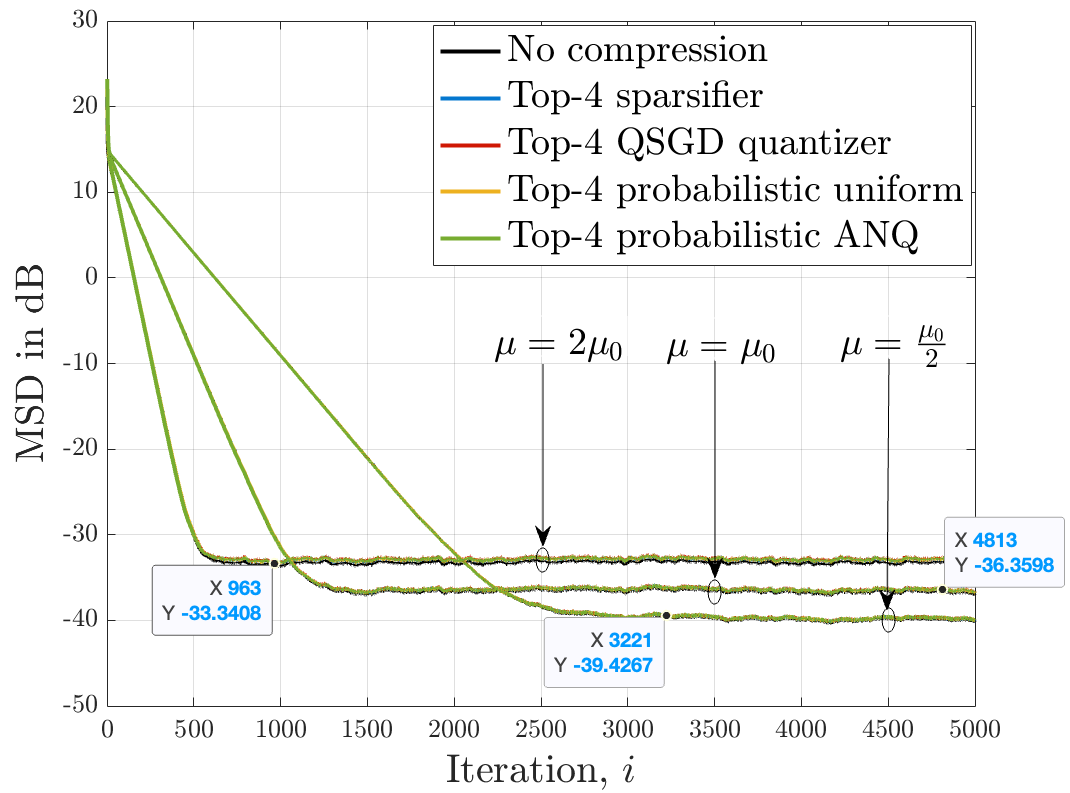
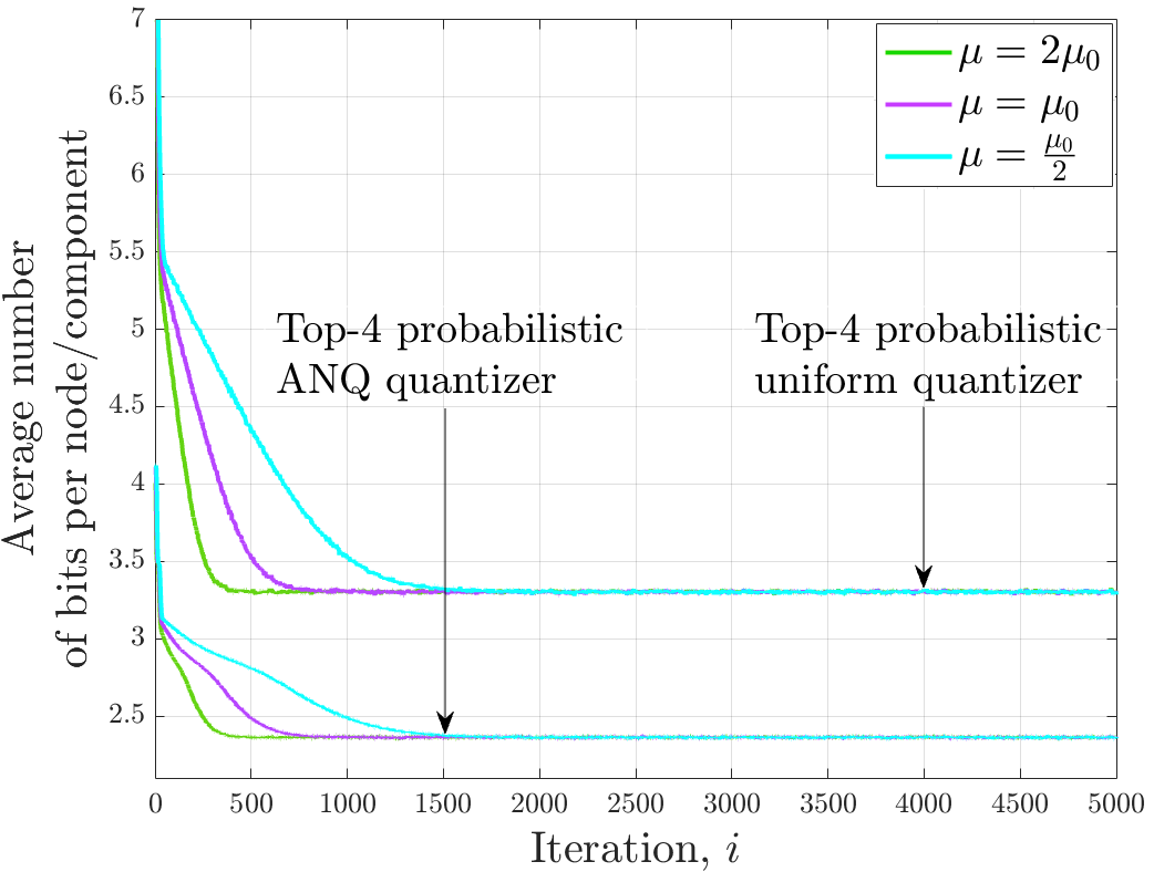
Figure 3: Network performance w.r.t. $w^{o}$ for three different values of the step-size ($\mu_{0}=0.001$). (Left) Evolution of the MSD learning curves. (Right) Evolution of the average number of bits per node, per component, when the variable-rate probabilistic uniform and ANQ schemes are used at the output of the top-$4$ sparsifier to encode the error compensated difference $\boldsymbol{\chi}_{k,i}=\boldsymbol{\psi}_{k,i}-\boldsymbol{\phi}_{k,i-1}+\boldsymbol{z}_{k,i-1}$ in (18b).

Evaluating the performance of a learning approach requires considering both the attained learning error (MSD) and the associated bit expense. Therefore, in the following, we focus on reporting rate-distortion (RD) curves, where the bit budget quantifies the rate and the MSD quantifies the distortion.

V-B Top-$c$ quantization outperforms other compression rules

We report in Fig. 4 the RD curves of the DEF-ATC approach with probabilistic uniform and top-$4$ probabilistic uniform quantization. We set $\mu=0.001$ and $\gamma=\zeta=0.9$. Each point of the rate-distortion curve corresponds to one value of the parameter $\varepsilon$, which determines the quantization step $\Delta=\mu^{\frac{1+\varepsilon}{2}}$. In the example, we selected $25$ values of $\varepsilon$ linearly spaced in the interval $[10^{-3},1]$. For each value of $\Delta$ (i.e., each point of the curve), the resulting MSD (distortion) and average number of bits/node/component (rate) were obtained by averaging the instantaneous mean-square-deviation $\text{MSD}(i)$ in (82) and averaging the number of bits $R(i)$ in (83) over $100$ samples after convergence of the algorithm (the expectations in (82) and (83) are estimated empirically over $100$ Monte Carlo runs). The trade-off between rate and distortion can be observed from Fig. 4, namely, as the rate decreases, the distortion increases, and vice versa. For comparison purposes, we illustrate in Fig. 4 the distortion (horizontal dashed line) of the uncompressed ATC approach obtained by averaging $\text{MSD}(i)$ in (82) over $100$ samples after convergence. We also illustrate the specific $\log_{2}(3)$ bit rate (vertical dashed line) corresponding to minimum number of bits possible for the considered scheme, namely, the variable-rate coding scheme from [25], [26, Sec. II]. Under this scheme, each component is appended with a parsing symbol, and the $0$ value is encoded as an empty element. Thus, the minimum number of bits/component would correspond to sending only one symbol per component. As it can be observed, top-$4$ probabilistic uniform is more efficient than probabilistic uniform, namely, it approaches the uncompressed performance (low distortion) at a lower bit rate compared to probabilistic uniform quantization.

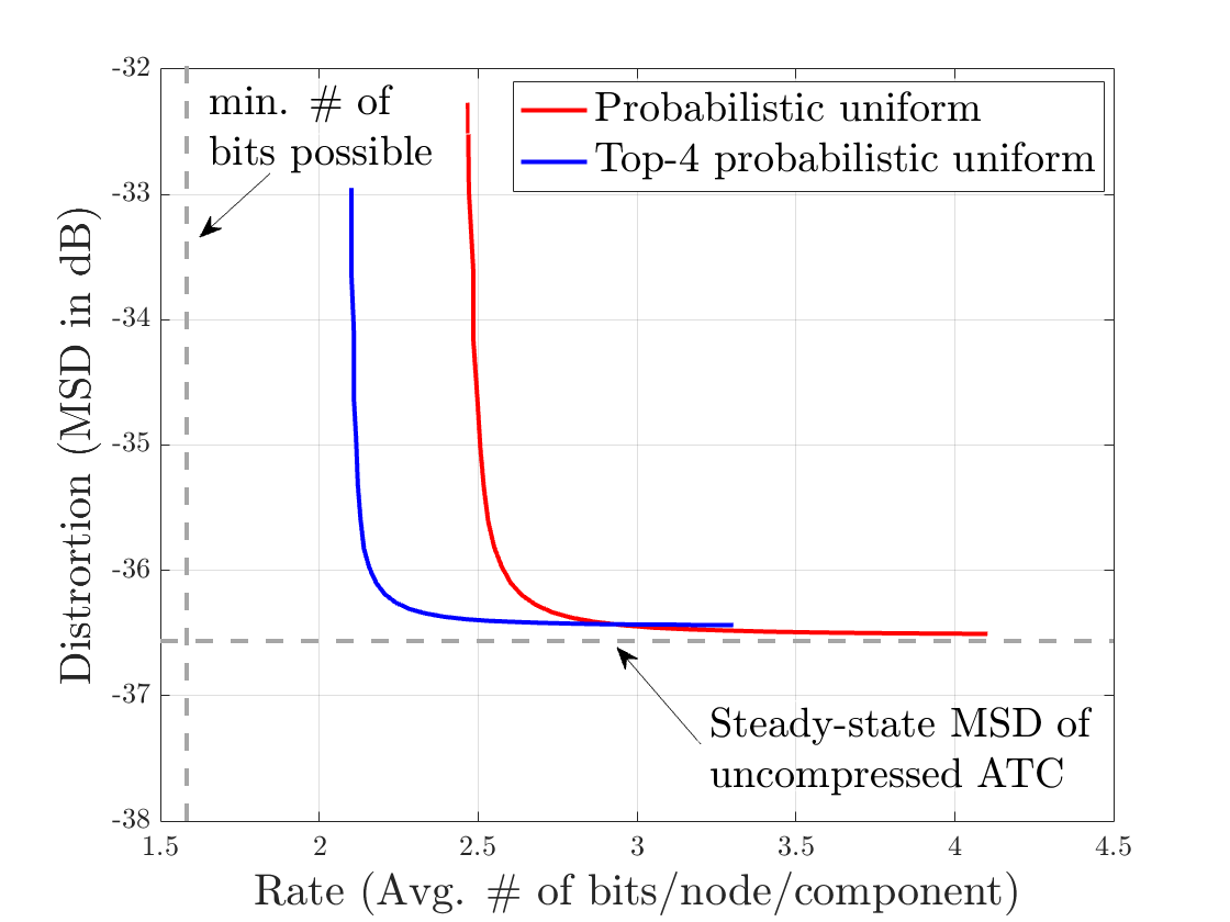
Figure 4: Rate-distortion curves of the DEF-ATC approach with probabilistic uniform and top-$4$ probabilistic uniform quantization.

V-C Performance w.r.t. state-of-the-art baselines

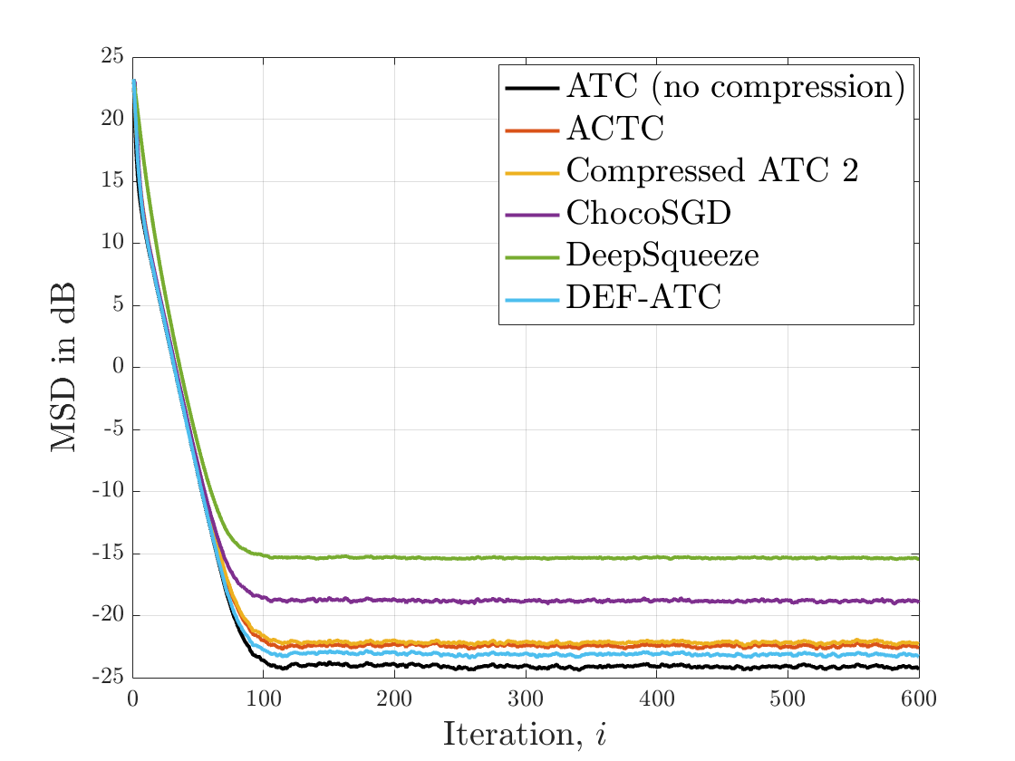
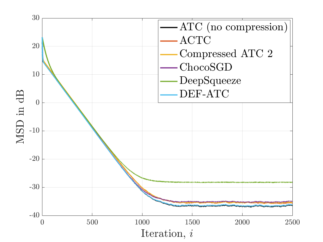
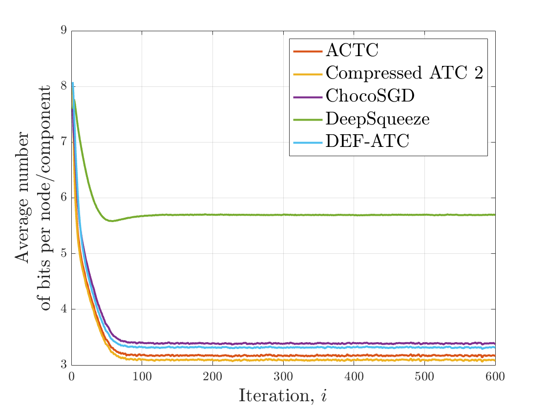
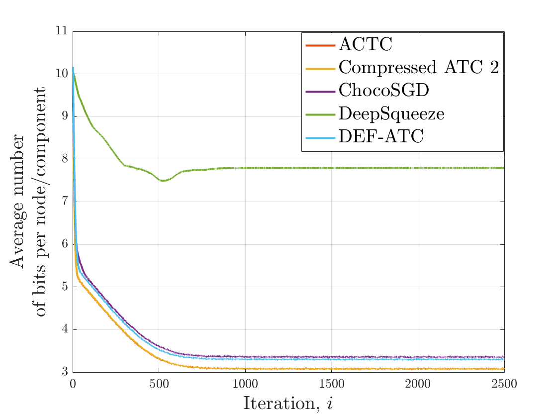
Figure 5: DEF-ATC performance w.r.t. to state-of-the-art baselines. Evolution of the MSD and average number of bits/node/component (when top-$4$ probabilistic uniform with variable-rate encoding scheme is used) for different values of the step-size. (Left) $\mu=0.01$. (Right) $\mu=0.001$.

In this part, we compare the DEF-ATC diffusion to the following approaches: $i)$ ChocoSGD [11], $ii)$ DeepSqueeze [33], $iii)$ diffusion ACTC [21], and $iv)$ compressed diffusion ATC approach (which we refer to as the “compressed ATC $2$”) [26]. We assume that all agents employ the top-$4$ probabilistic uniform quantizer with the variable rate encoding scheme from [25], [26, Sec. II]. In Fig. 5, we report the network MSD learning curves with the corresponding bit rates, for 2 different values of the step-size $\mu=0.01$ (left) and $\mu=0.001$ (right). The results are averaged over $100$ Monte-Carlo runs. We set the quantization parameter $\Delta=\mu$. For the ACTC [21] and compressed ATC $2$ [26] approaches (which were originally designed to handle unbiased probabilistic compression), we used a step-size $\mu=0.0125$ and $\mu=0.00125$, in place of $\mu=0.01$ and $\mu=0.001$, respectively, in order to ensure that they have the same learning rate as the uncompressed ATC approach. This configuration ensures that all approaches are compared at the same learning rate. The other parameters of the baselines approaches are set as follows: $i)$ ChocoSGD: $\gamma=0.9$, $ii)$ DeepSqueeze: (consensus parameter) $\eta=0.05$ when $\mu=0.01$ and $\eta=0.2$ when $\mu=0.001$, $iii)$ ACTC: $\zeta=0.9$, $iv)$ compressed ATC $2$: $\gamma=0.9$, and $v)$ DEF-ATC: $\gamma=\zeta=0.9$. While the space of algorithms’ hyperparameters ($\gamma$, $\zeta$, etc.) is explored in the next experiment, it is worth noting that the values chosen in the current experiment ensure a stable compressed strategy with the lowest MSD level. As it can be observed from the MSD learning curves, the DEF-ATC approach tends to outperform state-of-the-art baselines in various step-size regimes. In order to identify which method provides better compression efficiency for a given level of distortion, we report in Fig. 6 the RD curves of the different approaches. Before analyzing the results, it is noteworthy that the bit rate curves reported in Fig. 5 indicate that the DeepSqueeze approach tends to require a larger number of bits as the step-size decreases. Thus, for very fine quantization (i.e., small step-sizes since $\Delta=\mu$), the number of bits required tends to grow, making it impractical for use in such scenarios. By noting that DeepSqueeze does not employ differential quantization, the increase in bit rate with decreasing quantization step is expected. In fact, in this case, the input values at the compressor remain large (in particular, their effective range does not scale with the step-size $\mu$), leading to an increase in the bit rate with decreasing quantization step.

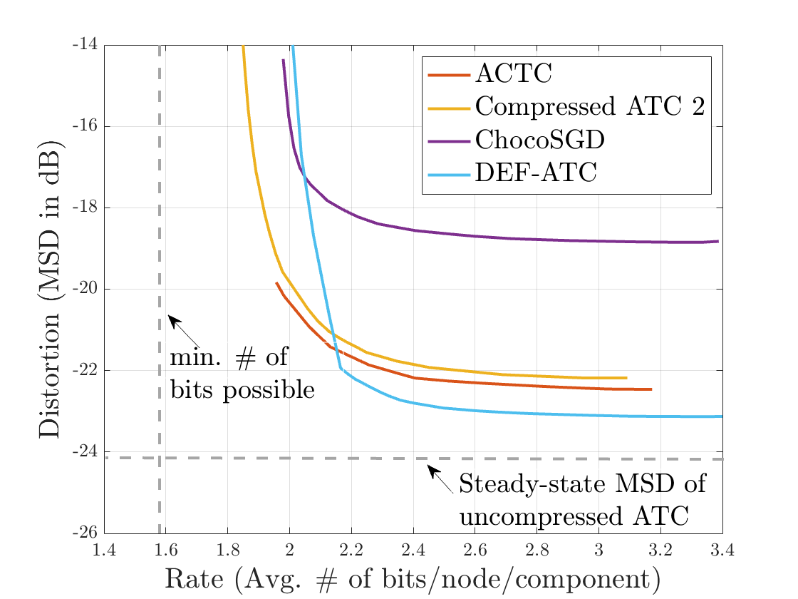
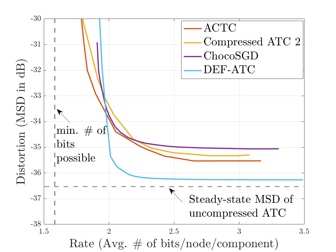
Figure 6: Rate-distortion curves of the DEF-ATC and state-of-the-art baselines approaches for different values of the step-size. The top-$4$ probabilistic uniform quantizer with variable-rate encoding scheme is used. (Left) $\mu=0.01$. (Right) $\mu=0.001$.

For each approach, the process for generating the rate-distortion curves in Fig. 6 consists of three main steps. First, we select a set of algorithm’s hyperparameters ($\gamma$, $\zeta$, etc.). In particular, for ACTC [21], we select $10$ values of the damping coefficient $\zeta$ uniformly spaced in the interval $[0.1,0.9]$. For compressed ATC $2$ [26] (and ChocoSGD [11]), we select $10$ values of the mixing parameter $\gamma$ uniformly spaced in the interval $[0.1,0.9]$. For the DEF-ATC approach, we create two sets of $5$ uniformly spaced values in the interval $[0.1,0.9]$ for the coefficients $\zeta$ and $\gamma$, and then consider all possible pairs from these sets. In the second step, and for each hyperparameter setting (i.e., each element in the sets of step 1), we generate the RD curve by following the same method as in Sec. V-B, namely, we vary the quantization step according to $\Delta=\mu^{\frac{1+\varepsilon}{2}}$, where $25$ values of $\varepsilon$ linearly spaced in the interval $[10^{-3},1]$ are chosen. For each value of $\Delta$, distortion and rate are evaluated by averaging over $100$ samples after convergence (expectations are computed empirically over $50$ Monte Carlo runs). Each RD curve then represents the performance of the algorithm under a specific choice of hyperparameters. In the last step, we generate and report in Fig. 6 the optimal RD curve given by the convex hull of the empirical curves collected in step $2$. This process allows us to identify the best possible performance trade-offs by varying the algorithms’ hyperparameters ($\gamma$, $\zeta$, etc.) and the compression parameters, namely, $\varepsilon$. Two learning step-size regimes are considered, namely, $\mu=0.01$ (left plot) and $\mu=0.001$ (right plot). By exploring the hyperparameter space and by considering different step-size regimes, the results show that the DEF-ATC approach can still achieve the closest performance to the uncompressed approach with a relatively small number of bits (approximately $2.2$–$2.4$ bits/component/iteration are required on average in steady-state), outperforming state-of-the-art baselines.

V-D Beyond single-task estimation

To illustrate the effectiveness of the DEF-ATC approach in solving general optimization problems of the form (2), we conduct an experiment in which agents seek consensus on certain components of their estimates while seeking partial consensus on others. In particular, we assume that we have $5$ connected groups of agents, namely, $\mathcal{G}_{1}=\{1,\ldots,15\}$, $\mathcal{G}_{2}=\{16,\ldots,30\}$, $\mathcal{G}_{3}=\{1,\ldots,10\}$, $\mathcal{G}_{4}=\{11,\ldots,20\}$, and $\mathcal{G}_{5}=\{21,\ldots,30\}$, and that the model parameter vector $w^{\star}_{k}$ at agent $k$ is of the form $w^{\star}_{k}=w^{\bullet}_{k}+\Delta_{k,i}$, where $\Delta_{k,i}$ is a $10\times 1$ vector with each component randomly generated from the Gaussian distribution, with zero mean and variance $0.1$. The vectors $\{w^{\bullet}_{k}\}$ are generated in such a way that the first $5$ components are common across the network, the components $6,7,8$ are separately common for agents in $\mathcal{G}_{1}$ and $\mathcal{G}_{2}$, and the last two components are separately common for agents in groups $\mathcal{G}_{3},\mathcal{G}_{4}$, and $\mathcal{G}_{5}$. Then, we choose the constraints in (2) (i.e., the matrix $\mathcal{U}$) in order to enforce global consensus on the first $5$ components of the estimates and partial consensus on the remaining components. The partial consensus is as follows. Agents in $\mathcal{G}_{1}$ should converge to a consensus on components $6$–$8$, and agents in $\mathcal{G}_{2}$ should also converge to a consensus on components $6$–$8$, independently from the first group. For the remaining two components $9$ and $10$, consensus is enforced within each of the groups $\mathcal{G}_{3},\mathcal{G}_{4}$, and $\mathcal{G}_{5}$. The matrix $\mathcal{A}$ satisfying the conditions in (4) and having the same sparsity structure as the link matrix in Fig. 2 (left) is found by following the same approach as in [40].We assume that all agents employ the top-$4$ probabilistic uniform quantizer. In Fig. 7 (left) and (middle), we report the network MSD (82) and average number of bits/node/component (83) for $3$ different values of the step-size $\mu$. The results are averaged over $100$ Monte-Carlo runs. We set $\gamma=\zeta=0.9$ and the quantizer parameter $\Delta=\mu$. As in Sec. V-A, we observe, in the small step-size regime, that the DEF-ATC achieves the same performance (which is on the order of $\mu$) as the uncompressed ATC approach, and is able to maintain a finite bit rate when the step-size approaches zero. This illustrates the effectiveness of DEF-ATC in handling different problem settings, beyond traditional single-task estimation. In Fig. 7 (right), we report the RD curves of DEF-ATC with probabilistic uniform and top-$4$ probabilistic uniform quantization. These curves have been generated in the same way as those in Fig. 4. The results show that quantizing only the highest magnitude components of a vector, as opposed to the entire vector, can reduce the number of bits required while maintaining a low level of distortion.

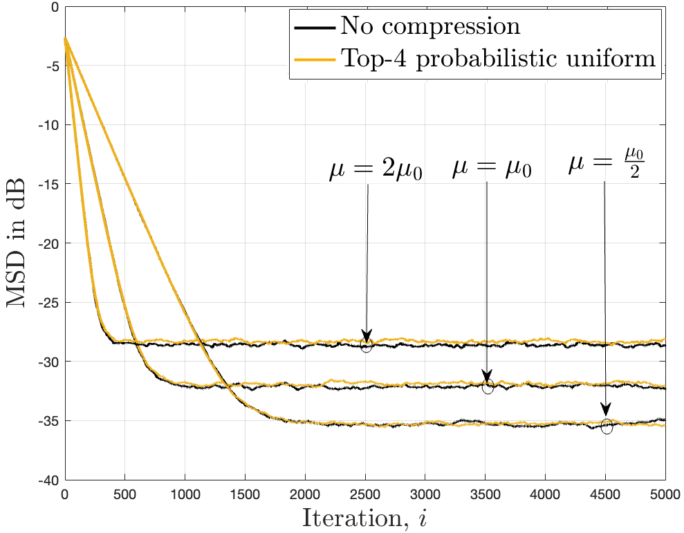
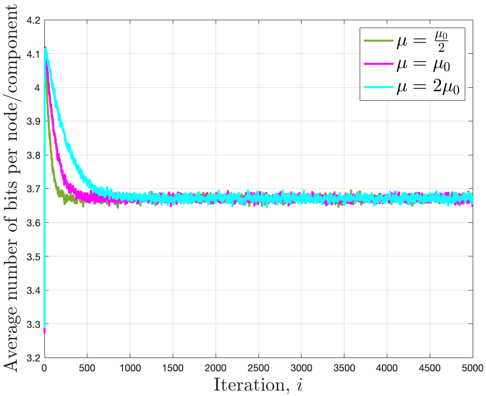
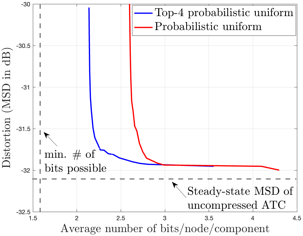
Figure 7: Beyond single-task estimation. (Left) Network MSD learning curves w.r.t. $w^{o}_{k}$ in (2) for three different values of the step-size ($\mu_{0}=0.001$). (Middle) Evolution of the average number of bits/node/component when the variable-rate scheme is used. (Right) Rate-distortion curves of the DEF-ATC (when $\mu=\mu_{0}$) with probabilistic uniform and top-$4$ probabilistic uniform quantization.

VI Conclusion

In this work, we presented an approach for solving decentralized learning problems where agents have individual risks to minimize subject to subspace constraints that require the minimizers across the network to lie in low-dimensional subspaces. This constrained formulation includes consensus or single-task optimization as a special case, and allows for more general task relatedness models such as multitask smoothness and coupled optimization. To reduce the communication cost among agents, we incorporated compression into the decentralized approach by employing differential quantization at the agent level to compress the iterates before communicating them to neighbors. In addition, we implemented in the learning approach an error-feedback mechanism, which consists of incorporating the compression error into subsequent steps. We then showed that, under some general conditions on the compression noise, and for sufficiently small step-sizes $\mu$, the resulting communication-efficient strategy is stable both in terms of mean-square error and average bit rate. The results showed that, in the small step-size regime, the iterates generated by the decentralized communication-efficient approach achieve the same performance as the decentralized baseline full-precision approach where no communication compression is performed. Simulations illustrated the theoretical findings and the effectiveness of the approach.

Appendix A Proof of Lemma 1

Let $\mathcal{I}^{\prime}_{c}$ denote the complement set of $\mathcal{I}_{c}$. Since all the components $\{x_{j},j\in\mathcal{I}_{c}\}$ are in magnitude greater than or equal to the components $\{x_{j},j\in\mathcal{I}^{\prime}_{c}\}$, we can write:

$$\frac{1}{c}\sum_{j\in\mathcal{I}_{c}}x_{j}^{2}\geq\frac{1}{L}\sum_{j=1}^{L}x_{j}^{2},$$ (84)

from which we conclude the following useful identity:

$$\sum_{j\in\mathcal{I}_{c}}x_{j}^{2}\geq\frac{c}{L}\|x\|^{2}.$$ (85)

Now, to show that the top-$c$ quantizer is a bounded-distortion compression operator with parameters given by (12), we can manipulate the compression error as follows:

$$\mathbb{E}\|x-\boldsymbol{\cal{C}}(x)\|^{2}=\mathbb{E}\|x-\alpha\boldsymbol{\cal{Q}}(\mathcal{S}(x))\|^{2} =\mathbb{E}\|x-\alpha\mathcal{S}(x)+\alpha(\mathcal{S}(x)-\boldsymbol{\cal{Q}}(\mathcal{S}(x)))\|^{2}$$

$$\overset{\text{(a)}}{=}\|x-\alpha\mathcal{S}(x)\|^{2}+\alpha^{2}\mathbb{E}\|\mathcal{S}(x)-\boldsymbol{\cal{Q}}(\mathcal{S}(x))\|^{2}$$

$$\leq\|x-\alpha\mathcal{S}(x)\|^{2}+\alpha^{2}\beta^{2}_{q}\|\mathcal{S}(x)\|^{2}+\alpha^{2}\sigma^{2}_{q}$$

$$=(1-\alpha)^{2}\sum_{j\in\mathcal{I}_{c}}x_{j}^{2}+\sum_{j\in\mathcal{I}^{\prime}_{c}}\|x_{j}\|^{2}+\alpha^{2}\beta^{2}_{q}\|\mathcal{S}(x)\|^{2}+\alpha^{2}\sigma^{2}_{q}$$

$$=\left((1-\alpha)^{2}+\alpha^{2}\beta^{2}_{q}\right)\sum_{j\in\mathcal{I}_{c}}x_{j}^{2}+\sum_{j\in\mathcal{I}^{\prime}_{c}}\|x_{j}\|^{2}+\alpha^{2}\sigma^{2}_{q}$$

$$=\|x\|^{2}-\left(1-\left((1-\alpha)^{2}+\alpha^{2}\beta^{2}_{q}\right)\right)\sum_{j\in\mathcal{I}_{c}}\|x_{j}\|^{2}+\alpha^{2}\sigma^{2}_{q}$$

$$\overset{\eqref{eq: intermediate equation for the sparsifier}}{\leq}\left(1-\left(1-\left((1-\alpha)^{2}+\alpha^{2}\beta^{2}_{q}\right)\right)\frac{c}{L}\right)\|x\|^{2}+\alpha^{2}\sigma^{2}_{q},$$ (86)

where in (a) we used the fact that $\alpha\langle x-\alpha\mathcal{S}(x),\mathbb{E}[\mathcal{S}(x)-\boldsymbol{\cal{Q}}(\mathcal{S}(x))]\rangle=0$ in both cases: biased ($\alpha=1$) and unbiased ($\alpha=\frac{1}{1+\beta^{2}_{q}}$) quantizer $\boldsymbol{\cal{Q}}(\cdot)$.

Appendix B Mean-square-error analysis

We consider the transformed iterates $\overline{\boldsymbol{\phi}}^{z}_{i}$ and $\widecheck{\boldsymbol{\phi}}^{z}_{i}$ in (65) and (66), respectively. Computing the second-order moment of both sides of (65), we get:

$$\mathbb{E}\|\overline{\boldsymbol{\phi}}^{z}_{i}\|^{2}=\mathbb{E}\|(I_{P}-\mu\boldsymbol{\cal{D}}_{11,i-1})\overline{\boldsymbol{\phi}}^{z}_{i-1}-\mu\boldsymbol{\cal{D}}_{12,i-1}\widecheck{\boldsymbol{\phi}}^{z}_{i-1}-\mu\boldsymbol{\cal{D}}_{11,i-1}\overline{\boldsymbol{z}}_{i-1}-\mu\boldsymbol{\cal{D}}_{12,i-1}\widecheck{\boldsymbol{z}}_{i-1}\|^{2}+\mu^{2}\mathbb{E}\|\overline{\boldsymbol{s}}_{i}\|^{2},$$ (87)

where, from Assumption 2 on the gradient noise processes, we used the fact that:

$$\mathbb{E}[\boldsymbol{x}_{i-1}^{\top}\overline{\boldsymbol{s}}_{i}] =\mathbb{E}\left[\mathbb{E}\left[\boldsymbol{x}_{i-1}^{\top}\overline{\boldsymbol{s}}_{i}\Big{|}\{{\boldsymbol{\phi}_{\ell,i-1},\boldsymbol{z}_{\ell,i-1}}\}_{\ell=1}^{K}\right]\right]=\mathbb{E}\left[\boldsymbol{x}_{i-1}^{\top}\mathbb{E}\left[\overline{\boldsymbol{s}}_{i}\Big{|}\{{\boldsymbol{\phi}_{\ell,i-1},\boldsymbol{z}_{\ell,i-1}}\}_{\ell=1}^{K}\right]\right]=0$$ (88)

with $\boldsymbol{x}_{i-1}=(I_{P}-\mu\boldsymbol{\cal{D}}_{11,i-1})\overline{\boldsymbol{\phi}}^{z}_{i-1}-\mu\boldsymbol{\cal{D}}_{12,i-1}\widecheck{\boldsymbol{\phi}}^{z}_{i-1}-\mu\boldsymbol{\cal{D}}_{11,i-1}\overline{\boldsymbol{z}}_{i-1}-\mu\boldsymbol{\cal{D}}_{12,i-1}\widecheck{\boldsymbol{z}}_{i-1}$. Using similar arguments, we can also show that:

$$\mathbb{E}\|\widecheck{\boldsymbol{\phi}}^{z}_{i}\|^{2}= \mathbb{E}\|(\mathcal{J}^{\prime\prime}_{\epsilon}-\mu\boldsymbol{\cal{D}}_{22,i-1})\widecheck{\boldsymbol{\phi}}^{z}_{i-1}-\mu\boldsymbol{\cal{D}}_{21,i-1}\overline{\boldsymbol{\phi}}^{z}_{i-1}+\mu\widecheck{b}-\mu\boldsymbol{\cal{D}}_{21,i-1}\overline{\boldsymbol{z}}_{i-1}-\left(\zeta(I-\mathcal{J}_{\epsilon}^{\prime})+\mu\boldsymbol{\cal{D}}_{22,i-1}\right)\widecheck{\boldsymbol{z}}_{i-1}\|^{2}$$

$$\qquad\qquad\qquad+\mu^{2}\mathbb{E}\|\widecheck{\boldsymbol{s}}_{i}\|^{2}.$$ (89)

By using similar arguments as those used to establish inequalities (119) and (124) in [40, Appendix D], we can show that:

$$\begin{split}\mathbb{E}\|\overline{\boldsymbol{\phi}}^{z}_{i}\|^{2}&\leq(1-\mu\sigma_{11})\mathbb{E}\|\overline{\boldsymbol{\phi}}^{z}_{i-1}\|^{2}+\frac{\mu}{\sigma_{11}}\mathbb{E}\|\boldsymbol{\cal{D}}_{12,i-1}\widecheck{\boldsymbol{\phi}}^{z}_{i-1}+\boldsymbol{\cal{D}}_{11,i-1}\overline{\boldsymbol{z}}_{i-1}+\boldsymbol{\cal{D}}_{12,i-1}\widecheck{\boldsymbol{z}}_{i-1}\|^{2}+\mu^{2}\mathbb{E}\|\overline{\boldsymbol{s}}_{i}\|^{2}\\ &\leq(1-\mu\sigma_{11})\mathbb{E}\|\overline{\boldsymbol{\phi}}^{z}_{i-1}\|^{2}+\frac{3\mu\sigma^{2}_{12}}{\sigma_{11}}\mathbb{E}\|\widecheck{\boldsymbol{\phi}}^{z}_{i-1}\|^{2}+3\mu\sigma_{11}\mathbb{E}\|\overline{\boldsymbol{z}}_{i-1}\|^{2}+\frac{3\mu\sigma^{2}_{12}}{\sigma_{11}}\mathbb{E}\|\widecheck{\boldsymbol{z}}_{i-1}\|^{2}+\mu^{2}\mathbb{E}\|\overline{\boldsymbol{s}}_{i}\|^{2}\\ &\leq(1-\mu\sigma_{11})\mathbb{E}\|\overline{\boldsymbol{\phi}}^{z}_{i-1}\|^{2}+\frac{3\mu\sigma^{2}_{12}}{\sigma_{11}}\mathbb{E}\|\widecheck{\boldsymbol{\phi}}^{z}_{i-1}\|^{2}+\left(3\mu\sigma_{11}+\frac{3\mu\sigma^{2}_{12}}{\sigma_{11}}\right)\mathbb{E}\|\mathcal{V}_{\epsilon}^{-1}\boldsymbol{z}_{i-1}\|^{2}+{\mu^{2}}\mathbb{E}\|\overline{\boldsymbol{s}}_{i}\|^{2},\end{split}$$ (90)

and

$$\begin{split}\mathbb{E}\|\widecheck{\boldsymbol{\phi}}^{z}_{i}\|^{2}&\leq\|\mathcal{J}^{\prime\prime}_{\epsilon}\|\mathbb{E}\|\widecheck{\boldsymbol{\phi}}^{z}_{i-1}\|^{2}+\frac{2\mu^{2}}{1-\|\mathcal{J}^{\prime\prime}_{\epsilon}\|}\mathbb{E}\|\boldsymbol{\cal{D}}_{22,i-1}\widecheck{\boldsymbol{\phi}}^{z}_{i-1}+\boldsymbol{\cal{D}}_{21,i-1}\overline{\boldsymbol{\phi}}^{z}_{i-1}-\widecheck{b}+\boldsymbol{\cal{D}}_{21,i-1}\overline{\boldsymbol{z}}_{i-1}+\boldsymbol{\cal{D}}_{22,i-1}\widecheck{\boldsymbol{z}}_{i-1}\|^{2}+\\ &\qquad\frac{2\zeta^{2}\|I-\mathcal{J}_{\epsilon}^{\prime}\|^{2}}{1-\|\mathcal{J}^{\prime\prime}_{\epsilon}\|}\mathbb{E}\|\widecheck{\boldsymbol{z}}_{i-1}\|^{2}+\mu^{2}\mathbb{E}\|\widecheck{\boldsymbol{s}}_{i}\|^{2}\\ &\leq\left(\|\mathcal{J}^{\prime\prime}_{\epsilon}\|+\frac{10\mu^{2}\sigma_{22}^{2}}{1-\|\mathcal{J}^{\prime\prime}_{\epsilon}\|}\right)\mathbb{E}\|\widecheck{\boldsymbol{\phi}}^{z}_{i-1}\|^{2}+\left(\frac{10\mu^{2}\sigma_{21}^{2}}{1-\|\mathcal{J}^{\prime\prime}_{\epsilon}\|}\right)\mathbb{E}\|\overline{\boldsymbol{\phi}}^{z}_{i-1}\|^{2}+\left(\frac{10\mu^{2}}{1-\|\mathcal{J}^{\prime\prime}_{\epsilon}\|}\right)\|\widecheck{b}\|^{2}+\\ &\qquad\left(\frac{10\mu^{2}\sigma_{21}^{2}}{1-\|\mathcal{J}^{\prime\prime}_{\epsilon}\|}\right)\mathbb{E}\|\overline{\boldsymbol{z}}_{i-1}\|^{2}+\left(\frac{2\zeta^{2}\|I-\mathcal{J}_{\epsilon}^{\prime}\|^{2}}{1-\|\mathcal{J}^{\prime\prime}_{\epsilon}\|}+\frac{10\mu^{2}\sigma_{22}^{2}}{1-\|\mathcal{J}^{\prime\prime}_{\epsilon}\|}\right)\mathbb{E}\|\widecheck{\boldsymbol{z}}_{i-1}\|^{2}+\mu^{2}\mathbb{E}\|\widecheck{\boldsymbol{s}}_{i}\|^{2}\\ &\leq\left(\|\mathcal{J}^{\prime\prime}_{\epsilon}\|+\frac{10\mu^{2}\sigma_{22}^{2}}{1-\|\mathcal{J}^{\prime\prime}_{\epsilon}\|}\right)\mathbb{E}\|\widecheck{\boldsymbol{\phi}}^{z}_{i-1}\|^{2}+\left(\frac{10\mu^{2}\sigma_{21}^{2}}{1-\|\mathcal{J}^{\prime\prime}_{\epsilon}\|}\right)\mathbb{E}\|\overline{\boldsymbol{\phi}}^{z}_{i-1}\|^{2}+\left(\frac{10\mu^{2}}{1-\|\mathcal{J}^{\prime\prime}_{\epsilon}\|}\right)\|\widecheck{b}\|^{2}+\\ &\qquad\left(\frac{2{\zeta^{2}}\|I-\mathcal{J}_{\epsilon}^{\prime}\|^{2}}{1-\|\mathcal{J}^{\prime\prime}_{\epsilon}\|}+\frac{10\mu^{2}(\sigma_{22}^{2}+\sigma_{21}^{2})}{1-\|\mathcal{J}^{\prime\prime}_{\epsilon}\|}\right)\mathbb{E}\|\mathcal{V}_{\epsilon}^{-1}\boldsymbol{z}_{i-1}\|^{2}+\mu^{2}\mathbb{E}\|\widecheck{\boldsymbol{s}}_{i}\|^{2},\end{split}$$ (91)

for some positive constant $\sigma_{11}$ and non-negative constants $\sigma_{12},\sigma_{21}$, and $\sigma_{22}$ independent of $\mu$, and where we used the fact that the $2-$induced matrix norm of the block diagonal matrix $\mathcal{J}^{\prime\prime}_{\epsilon}$ in (71) satisfies $\|\mathcal{J}^{\prime\prime}_{\epsilon}\|\in(0,1)$. In fact, from (44), we can re-write $\mathcal{J}^{\prime\prime}_{\epsilon}$ in the following form:

$$\mathcal{J}^{\prime\prime}_{\epsilon}=(1-\gamma\zeta)I_{M-P}+\gamma\zeta\mathcal{J}_{\epsilon}.$$ (92)

By following similar arguments as in [6, pp. 516–517], we can first show that $\mathcal{J}^{\prime\prime}_{\epsilon}$ in (92) satisfies:

$$\|\mathcal{J}_{\epsilon}^{\prime\prime}\|^{2}\leq(\rho(\mathcal{J}^{\prime\prime}_{\epsilon})+\gamma\zeta\epsilon)^{2}.$$ (93)

From (92), we can also show that:

$$\rho(\mathcal{J}^{\prime\prime}_{\epsilon})\leq(1-\gamma\zeta)+\gamma\zeta\rho(\mathcal{J}_{\epsilon}).$$ (94)

Using the fact that $\rho(\mathcal{J}_{\epsilon})\in(0,1)$ from [40, Lemma 2] and the fact that $\gamma\zeta\in(0,1]$, we obtain $\rho(\mathcal{J}^{\prime\prime}_{\epsilon})\in(0,1)$. Moreover, since $\rho(\mathcal{J}^{\prime\prime}_{\epsilon})+\gamma\zeta\epsilon$ is non-negative, by replacing (94) into (93), we obtain:

$$\begin{split}\|\mathcal{J}_{\epsilon}^{\prime\prime}\|&\leq(1-\gamma\zeta)+\gamma\zeta\rho(\mathcal{J}_{\epsilon})+\gamma\zeta\epsilon\\ &=1-\gamma\zeta(1-\rho(\mathcal{J}_{\epsilon})-\epsilon).\end{split}$$ (95)

This identity will be used in the subsequent analysis. Returning to the result (91), and as it can be seen from (59), $\widecheck{b}=\mathcal{V}_{L,\epsilon}^{\top}b$ depends on $b$ in (27), which is defined in terms of the gradients $\{\nabla_{w_{k}}J_{k}(w^{o}_{k})\}$. Since the costs $J_{k}(w_{k})$ are twice differentiable, then $\|b\|^{2}$ is bounded and we obtain $\|\widecheck{b}\|^{2}=O(1)$.

For the gradient noise terms, by following similar arguments as in [6, Chapter 9], [40, Appendix D] and by using Assumption 2, we can show that:

$$\mathbb{E}\|\overline{\boldsymbol{s}}_{i}\|^{2}+\mathbb{E}\|\widecheck{\boldsymbol{s}}_{i}\|^{2}=\mathbb{E}\|\mathcal{V}_{\epsilon}^{-1}\boldsymbol{s}_{i}\|^{2}\leq v_{1}^{2}\beta_{s,\max}^{2}\mathbb{E}\|\widetilde{\boldsymbol{{\scriptstyle\mathcal{W}}}}_{i-1}\|^{2}+v_{1}^{2}\overline{\sigma}^{2}_{s},$$ (96)

where $v_{1}=\|\mathcal{V}_{\epsilon}^{-1}\|$, $\beta_{s,\max}^{2}=\max_{1\leq k\leq K}\beta_{s,k}^{2}$, and $\overline{\sigma}^{2}_{s}=\sum_{k=1}^{K}\sigma^{2}_{s,k}$. Using expression (33), the fact that $\widetilde{\boldsymbol{\phi}}_{i-1}=\widetilde{\boldsymbol{\phi}}^{z}_{i-1}+\boldsymbol{z}_{i-1}$, and the Jordan decomposition of the matrix $\mathcal{A}^{\prime}$ in (44), we obtain:

$$\mathbb{E}\|\overline{\boldsymbol{s}}_{i}\|^{2}+\mathbb{E}\|\widecheck{\boldsymbol{s}}_{i}\|^{2} \leq v_{1}^{2}\beta_{s,\max}^{2}\mathbb{E}\|\mathcal{A}^{\prime}(\widetilde{\boldsymbol{\phi}}^{z}_{i-1}+\boldsymbol{z}_{i-1})\|^{2}+v_{1}^{2}\overline{\sigma}^{2}_{s}$$

$$\leq v_{1}^{2}\beta_{s,\max}^{2}\mathbb{E}\|\mathcal{V}_{\epsilon}\Lambda^{\prime}(\mathcal{V}_{\epsilon}^{-1}\widetilde{\boldsymbol{\phi}}^{z}_{i-1}+\mathcal{V}_{\epsilon}^{-1}\boldsymbol{z}_{i-1})\|^{2}+v_{1}^{2}\overline{\sigma}^{2}_{s}$$

$$\overset{\text{(a)}}{\leq}v_{1}^{2}\beta_{s,\max}^{2}v_{2}^{2}(\mathbb{E}\|\mathcal{V}_{\epsilon}^{-1}\widetilde{\boldsymbol{\phi}}^{z}_{i-1}+\mathcal{V}_{\epsilon}^{-1}\boldsymbol{z}_{i-1}\|^{2})+v_{1}^{2}\overline{\sigma}^{2}_{s}$$

$$\leq 2v_{1}^{2}\beta_{s,\max}^{2}v_{2}^{2}(\mathbb{E}\|\overline{\boldsymbol{\phi}}^{z}_{i-1}\|^{2}+\mathbb{E}\|\widecheck{\boldsymbol{\phi}}^{z}_{i-1}\|^{2})+2v_{1}^{2}\beta_{s,\max}^{2}v_{2}^{2}\mathbb{E}\|\mathcal{V}_{\epsilon}^{-1}\boldsymbol{z}_{i-1}\|^{2}+v_{1}^{2}\overline{\sigma}^{2}_{s},$$ (97)

where $v_{2}=\|\mathcal{V}_{\epsilon}\|$. In step (a) we used the sub-multiplicative property of norms and the fact that the $2-$induced matrix norm of the block diagonal matrix $\Lambda^{\prime}$ in (44) is equal to $1$. Using the bound (97) into (90) and (91), we obtain:

$$\begin{split}\mathbb{E}\|\overline{\boldsymbol{\phi}}^{z}_{i}\|^{2}\leq&\left(1-\mu\sigma_{11}+2\mu^{2}v_{1}^{2}\beta_{s,\max}^{2}v_{2}^{2}\right)\mathbb{E}\|\overline{\boldsymbol{\phi}}^{z}_{i-1}\|^{2}+\left(\frac{3\mu\sigma^{2}_{12}}{\sigma_{11}}+2\mu^{2}v_{1}^{2}\beta_{s,\max}^{2}v_{2}^{2}\right)\mathbb{E}\|\widecheck{\boldsymbol{\phi}}^{z}_{i-1}\|^{2}+\\ &\left(3\mu\sigma_{11}+\frac{3\mu\sigma^{2}_{12}}{\sigma_{11}}+2\mu^{2}v_{1}^{2}\beta_{s,\max}^{2}v_{2}^{2}\right)\mathbb{E}\|\mathcal{V}_{\epsilon}^{-1}\boldsymbol{z}_{i-1}\|^{2}+\mu^{2}v_{1}^{2}\overline{\sigma}^{2}_{s},\end{split}$$ (98)

and

$$\begin{split}\mathbb{E}\|\widecheck{\boldsymbol{\phi}}^{z}_{i}\|^{2}\leq&\left(\|\mathcal{J}^{\prime\prime}_{\epsilon}\|+\frac{10\mu^{2}\sigma_{22}^{2}}{1-\|\mathcal{J}^{\prime\prime}_{\epsilon}\|}+2\mu^{2}v_{1}^{2}\beta_{s,\max}^{2}v_{2}^{2}\right)\mathbb{E}\|\widecheck{\boldsymbol{\phi}}^{z}_{i-1}\|^{2}+\left(\frac{10\mu^{2}\sigma_{21}^{2}}{1-\|\mathcal{J}^{\prime\prime}_{\epsilon}\|}+2\mu^{2}v_{1}^{2}\beta_{s,\max}^{2}v_{2}^{2}\right)\mathbb{E}\|\overline{\boldsymbol{\phi}}^{z}_{i-1}\|^{2}+\\ &\left(\frac{2\zeta^{2}\|I-\mathcal{J}_{\epsilon}^{\prime}\|^{2}}{1-\|\mathcal{J}^{\prime\prime}_{\epsilon}\|}+\frac{10\mu^{2}(\sigma_{22}^{2}+\sigma_{21}^{2})}{1-\|\mathcal{J}^{\prime\prime}_{\epsilon}\|}+2\mu^{2}v_{1}^{2}\beta_{s,\max}^{2}v_{2}^{2}\right)\mathbb{E}\|\mathcal{V}_{\epsilon}^{-1}\boldsymbol{z}_{i-1}\|^{2}+\left(\frac{10\mu^{2}}{1-\|\mathcal{J}^{\prime\prime}_{\epsilon}\|}\right)\|\widecheck{b}\|^{2}+\mu^{2}v_{1}^{2}\overline{\sigma}^{2}_{s}.\end{split}$$ (99)

Now, for the quantization noise vector $\boldsymbol{z}_{i}$ in (40), we have:

$$\begin{split}\mathbb{E}\|\mathcal{V}_{\epsilon}^{-1}\boldsymbol{z}_{i}\|^{2}\leq\zeta^{2}v_{1}^{2}\left(\sum_{k=1}^{K}\mathbb{E}\|\boldsymbol{z}_{k,i}\|^{2}\right).\end{split}$$ (100)

From (19) and Assumption 3, and since $\boldsymbol{\psi}_{k,i}-\boldsymbol{\phi}_{k,i-1}=\widetilde{\boldsymbol{\phi}}_{k,i-1}-\widetilde{\boldsymbol{\psi}}_{k,i}$, we can write:

$$\begin{split}\mathbb{E}\|\boldsymbol{z}_{k,i}\|^{2}\leq{\beta}^{2}_{c,k}\mathbb{E}\|\widetilde{\boldsymbol{\phi}}_{k,i-1}-\widetilde{\boldsymbol{\psi}}_{k,i}+\boldsymbol{z}_{k,i-1}\|^{2}+{\sigma}^{2}_{c,k},\end{split}$$ (101)

and, therefore,

$$\begin{split}{\sum_{k=1}^{K}\mathbb{E}\|\boldsymbol{z}_{k,i}\|^{2}}\leq{\beta}_{c,\max}^{2}\mathbb{E}\|\widetilde{\boldsymbol{\phi}}_{i-1}-\widetilde{\boldsymbol{\psi}}_{i}+\boldsymbol{z}_{i-1}\|^{2}+\overline{\sigma}^{2}_{c},\end{split}$$ (102)

where ${\beta}_{c,\max}^{2}=\max_{1\leq k\leq K}\{{\beta}^{2}_{c,k}\}$ and $\overline{\sigma}^{2}_{c}=\sum_{k=1}^{K}{\sigma}^{2}_{c,k}$. Since the analysis is facilitated by transforming the network vectors into the Jordan decomposition basis of the matrix $\mathcal{A}^{\prime}$, we proceed by noting that the term ${\sum_{k=1}^{K}\mathbb{E}\|\boldsymbol{z}_{k,i}\|^{2}}$ can be bounded as follows:

$$\begin{split}{\sum_{k=1}^{K}\mathbb{E}\|\boldsymbol{z}_{k,i}\|^{2}}&\overset{\eqref{eq: expression 4 biased}}{\leq}{\beta}_{c,\max}^{2}\mathbb{E}\|\mathcal{V}_{\epsilon}\mathcal{V}_{\epsilon}^{-1}(\widetilde{\boldsymbol{\phi}}_{i-1}-\widetilde{\boldsymbol{\psi}}_{i}+\boldsymbol{z}_{i-1})\|^{2}+\overline{\sigma}^{2}_{c}\\ &~{}\leq{\beta}_{c,\max}^{2}\|\mathcal{V}_{\epsilon}\|^{2}\mathbb{E}\|\mathcal{V}_{\epsilon}^{-1}(\widetilde{\boldsymbol{\phi}}_{i-1}-\widetilde{\boldsymbol{\psi}}_{i}+\boldsymbol{z}_{i-1})\|^{2}+\overline{\sigma}^{2}_{c}\\ &~{}=v_{2}^{2}{\beta}_{c,\max}^{2}\mathbb{E}\|\mathcal{V}_{\epsilon}^{-1}(\widetilde{\boldsymbol{\phi}}_{i-1}-\widetilde{\boldsymbol{\psi}}_{i}+\boldsymbol{z}_{i-1})\|^{2}+\overline{\sigma}^{2}_{c}\\ &~{}=v_{2}^{2}{\beta}_{c,\max}^{2}\left(\mathbb{E}\|\overline{\boldsymbol{\chi}}_{i}\|^{2}+\mathbb{E}\|\widecheck{\boldsymbol{\chi}}_{i}\|^{2}\right)+\overline{\sigma}^{2}_{c},\end{split}$$ (103)

where

$$\overline{\boldsymbol{\chi}}_{i} \triangleq\mathcal{U}^{\top}(\widetilde{\boldsymbol{\phi}}_{i-1}-\widetilde{\boldsymbol{\psi}}_{i}+\boldsymbol{z}_{i-1}),$$ (104)

$$\widecheck{\boldsymbol{\chi}}_{i} \triangleq\mathcal{V}_{L,\epsilon}^{\top}(\widetilde{\boldsymbol{\phi}}_{i-1}-\widetilde{\boldsymbol{\psi}}_{i}+\boldsymbol{z}_{i-1}).$$ (105)

Therefore, by combining (100) and (103), we obtain:

$$\begin{split}\mathbb{E}\|\mathcal{V}_{\epsilon}^{-1}\boldsymbol{z}_{i}\|^{2}\leq\zeta^{2}v_{1}^{2}v_{2}^{2}{\beta}_{c,\max}^{2}[\mathbb{E}\|\overline{\boldsymbol{\chi}}_{i}\|^{2}+\mathbb{E}\|\widecheck{\boldsymbol{\chi}}_{i}\|^{2}]+\zeta^{2}v_{1}^{2}\overline{\sigma}^{2}_{c}.\end{split}$$ (106)

We focus now on deriving the recursions that allow to examine the time-evolution of the transformed vectors $\overline{\boldsymbol{\chi}}_{i}$ and $\widecheck{\boldsymbol{\chi}}_{i}$. Subtracting $\widetilde{\boldsymbol{\phi}}_{i-1}$ from both sides of (31), adding $\boldsymbol{z}_{i-1}$, and using (33), we can write:

$$\widetilde{\boldsymbol{\phi}}_{i-1}-\widetilde{\boldsymbol{\psi}}_{i}+\boldsymbol{z}_{i-1} =\left(I_{M}-\left(I_{M}-\frac{\mu}{\zeta}\boldsymbol{\cal{H}}_{i-1}\right)\mathcal{A}^{\prime}\right)\widetilde{\boldsymbol{\phi}}_{i-1}+\frac{\mu}{\zeta}\boldsymbol{s}_{i}-\frac{\mu}{\zeta}b+\boldsymbol{z}_{i-1}$$

$$\overset{\text{(a)}}{=}\left(I_{M}-\left(I_{M}-\frac{\mu}{\zeta}\boldsymbol{\cal{H}}_{i-1}\right)\mathcal{A}^{\prime}\right)\widetilde{\boldsymbol{\phi}}^{z}_{i-1}+\frac{\mu}{\zeta}\boldsymbol{s}_{i}-\frac{\mu}{\zeta}b+\left(2I_{M}-\left(I_{M}-\frac{\mu}{\zeta}\boldsymbol{\cal{H}}_{i-1}\right)\mathcal{A}^{\prime}\right)\boldsymbol{z}_{i-1},$$ (107)

where in (a) we used the fact that $\widetilde{\boldsymbol{\phi}}_{i-1}=\widetilde{\boldsymbol{\phi}}^{z}_{i-1}+\boldsymbol{z}_{i-1}$. By multiplying both sides of (107) by $\mathcal{V}_{\epsilon}^{-1}$ and by using (49)–(64), (67)–(70), and the Jordan decomposition of the matrix $\mathcal{A}^{\prime}$, we obtain:

$$\begin{split}\left[\begin{array}[]{c}\overline{\boldsymbol{\chi}}_{i}\\ \widecheck{\boldsymbol{\chi}}_{i}\end{array}\right]=&\left[\begin{array}[]{cc}\frac{\mu}{\zeta}\boldsymbol{\cal{D}}_{11,i-1}&\frac{\mu}{\zeta}\boldsymbol{\cal{D}}_{12,i-1}\\ \frac{\mu}{\zeta}\boldsymbol{\cal{D}}_{21,i-1}&I_{M-P}-\mathcal{J}^{\prime}_{\epsilon}+\frac{\mu}{\zeta}\boldsymbol{\cal{D}}_{22,i-1}\end{array}\right]\left[\begin{array}[]{c}\overline{\boldsymbol{\phi}}^{z}_{i-1}\\ \widecheck{\boldsymbol{\phi}}^{z}_{i-1}\end{array}\right]+\frac{\mu}{\zeta}\left[\begin{array}[]{c}\overline{\boldsymbol{s}}_{i}\\ \widecheck{\boldsymbol{s}}_{i}\end{array}\right]-\frac{\mu}{\zeta}\left[\begin{array}[]{c}0\\ \widecheck{b}\end{array}\right]+\\ &\left[\begin{array}[]{cc}I_{P}+\frac{\mu}{\zeta}\boldsymbol{\cal{D}}_{11,i-1}&\frac{\mu}{\zeta}\boldsymbol{\cal{D}}_{12,i-1}\\ \frac{\mu}{\zeta}\boldsymbol{\cal{D}}_{21,i-1}&2I_{M-P}-\mathcal{J}^{\prime}_{\epsilon}+\frac{\mu}{\zeta}\boldsymbol{\cal{D}}_{22,i-1}\end{array}\right]\left[\begin{array}[]{c}\overline{\boldsymbol{z}}_{i-1}\\ \widecheck{\boldsymbol{z}}_{i-1}\end{array}\right].\end{split}$$ (108)

Again, by using similar arguments as those used to establish inequalities (119) and (124) in [40, Appendix D], we can verify that:

$$\begin{split}\mathbb{E}\|\overline{\boldsymbol{\chi}}_{i}\|^{2}&=\mathbb{E}\left\|(I_{P}+\frac{\mu}{\zeta}\boldsymbol{\cal{D}}_{11,i-1})\overline{\boldsymbol{z}}_{i-1}+\frac{\mu}{\zeta}\boldsymbol{\cal{D}}_{12,i-1}\widecheck{\boldsymbol{z}}_{i-1}+\frac{\mu}{\zeta}\boldsymbol{\cal{D}}_{11,i-1}\overline{\boldsymbol{\phi}}^{z}_{i-1}+\frac{\mu}{\zeta}\boldsymbol{\cal{D}}_{12,i-1}\widecheck{\boldsymbol{\phi}}^{z}_{i-1}\right\|^{2}+\frac{\mu^{2}}{\zeta^{2}}\mathbb{E}\|\overline{\boldsymbol{s}}_{i}\|^{2}\\ &\leq 2(1+\frac{\mu}{\zeta}\sigma_{11})^{2}\mathbb{E}\|\overline{\boldsymbol{z}}_{i-1}\|^{2}+\frac{2\mu^{2}}{\zeta^{2}}\mathbb{E}\|\boldsymbol{\cal{D}}_{12,i-1}\widecheck{\boldsymbol{z}}_{i-1}+\boldsymbol{\cal{D}}_{11,i-1}\overline{\boldsymbol{\phi}}^{z}_{i-1}+\boldsymbol{\cal{D}}_{12,i-1}\widecheck{\boldsymbol{\phi}}^{z}_{i-1}\|^{2}+\frac{\mu^{2}}{\zeta^{2}}\mathbb{E}\|\overline{\boldsymbol{s}}_{i}\|^{2}\\ &\leq 2(1+\frac{\mu}{\zeta}\sigma_{11})^{2}\mathbb{E}\|\overline{\boldsymbol{z}}_{i-1}\|^{2}+\frac{6\mu^{2}\sigma^{2}_{12}}{\zeta^{2}}\mathbb{E}\|\widecheck{\boldsymbol{z}}_{i-1}\|^{2}+\frac{6\mu^{2}\sigma^{2}_{11}}{\zeta^{2}}\mathbb{E}\|\overline{\boldsymbol{\phi}}^{z}_{i-1}\|^{2}+\frac{6\mu^{2}\sigma^{2}_{12}}{\zeta^{2}}\mathbb{E}\|\widecheck{\boldsymbol{\phi}}^{z}_{i-1}\|^{2}+\frac{\mu^{2}}{\zeta^{2}}\mathbb{E}\|\overline{\boldsymbol{s}}_{i}\|^{2}\\ &\overset{\text{(a)}}{\leq}\left(2(1+\frac{\mu}{\zeta}\sigma_{11})^{2}+\frac{6\mu^{2}\sigma^{2}_{12}}{\zeta^{2}}\right)\mathbb{E}\|\mathcal{V}_{\epsilon}^{-1}\boldsymbol{z}_{i-1}\|^{2}+\frac{6\mu^{2}\sigma^{2}_{11}}{\zeta^{2}}\mathbb{E}\|\overline{\boldsymbol{\phi}}^{z}_{i-1}\|^{2}+\frac{6\mu^{2}\sigma^{2}_{12}}{\zeta^{2}}\mathbb{E}\|\widecheck{\boldsymbol{\phi}}^{z}_{i-1}\|^{2}+\frac{\mu^{2}}{\zeta^{2}}\mathbb{E}\|\overline{\boldsymbol{s}}_{i}\|^{2},\end{split}$$ (109)

and

$$\begin{split}\mathbb{E}\|\widecheck{\boldsymbol{\chi}}_{i}\|^{2}&=\mathbb{E}\left\|(2I-\mathcal{J}^{\prime}_{\epsilon})\widecheck{\boldsymbol{z}}_{i-1}+\frac{\mu}{\zeta}\boldsymbol{\cal{D}}_{22,i-1}\widecheck{\boldsymbol{z}}_{i-1}+\frac{\mu}{\zeta}\boldsymbol{\cal{D}}_{21,i-1}\overline{\boldsymbol{z}}_{i-1}+\frac{\mu}{\zeta}\boldsymbol{\cal{D}}_{21,i-1}\overline{\boldsymbol{\phi}}^{z}_{i-1}+(I-\mathcal{J}^{\prime}_{\epsilon})\widecheck{\boldsymbol{\phi}}^{z}_{i-1}+\frac{\mu}{\zeta}\boldsymbol{\cal{D}}_{22,i-1}\widecheck{\boldsymbol{\phi}}^{z}_{i-1}-\frac{\mu}{\zeta}\widecheck{b}\right\|^{2}\\ &\qquad+\frac{\mu^{2}}{\zeta^{2}}\mathbb{E}\|\widecheck{\boldsymbol{s}}_{i}\|^{2}\\ &\leq 2\|2I-\mathcal{J}^{\prime}_{\epsilon}\|^{2}\mathbb{E}\|\widecheck{\boldsymbol{z}}_{i-1}\|^{2}+\frac{4\mu^{2}}{\zeta^{2}}\mathbb{E}\|\boldsymbol{\cal{D}}_{22,i-1}\widecheck{\boldsymbol{z}}_{i-1}+\boldsymbol{\cal{D}}_{21,i-1}\overline{\boldsymbol{z}}_{i-1}+\boldsymbol{\cal{D}}_{21,i-1}\overline{\boldsymbol{\phi}}^{z}_{i-1}+\boldsymbol{\cal{D}}_{22,i-1}\widecheck{\boldsymbol{\phi}}^{z}_{i-1}-\widecheck{b}\|^{2}+\\ &\qquad 4\|I-\mathcal{J}^{\prime}_{\epsilon}\|^{2}\mathbb{E}\|\widecheck{\boldsymbol{\phi}}^{z}_{i-1}\|^{2}+\frac{\mu^{2}}{\zeta^{2}}\mathbb{E}\|\widecheck{\boldsymbol{s}}_{i}\|^{2}\\ &\leq\left(2\|2I-\mathcal{J}^{\prime}_{\epsilon}\|^{2}+\frac{20\mu^{2}\sigma^{2}_{22}}{\zeta^{2}}\right)\mathbb{E}\|\widecheck{\boldsymbol{z}}_{i-1}\|^{2}+\frac{20\mu^{2}\sigma^{2}_{21}}{\zeta^{2}}\mathbb{E}\|\overline{\boldsymbol{z}}_{i-1}\|^{2}+\frac{20\mu^{2}\sigma^{2}_{21}}{\zeta^{2}}\mathbb{E}\|\overline{\boldsymbol{\phi}}^{z}_{i-1}\|^{2}+\frac{20\mu^{2}}{\zeta^{2}}\|\widecheck{b}\|^{2}+\\ &\qquad\left(4\|I-\mathcal{J}^{\prime}_{\epsilon}\|^{2}+\frac{20\mu^{2}\sigma^{2}_{22}}{\zeta^{2}}\right)\mathbb{E}\|\widecheck{\boldsymbol{\phi}}^{z}_{i-1}\|^{2}+\frac{\mu^{2}}{\zeta^{2}}\mathbb{E}\|\widecheck{\boldsymbol{s}}_{i}\|^{2}\\ &\overset{\text{(b)}}{\leq}\left(2\|2I-\mathcal{J}^{\prime}_{\epsilon}\|^{2}+\frac{20\mu^{2}(\sigma^{2}_{22}+\sigma^{2}_{21})}{\zeta^{2}}\right)\mathbb{E}\|\mathcal{V}_{\epsilon}^{-1}\boldsymbol{z}_{i-1}\|^{2}+\frac{20\mu^{2}\sigma^{2}_{21}}{\zeta^{2}}\mathbb{E}\|\overline{\boldsymbol{\phi}}^{z}_{i-1}\|^{2}+\frac{20\mu^{2}}{\zeta^{2}}\|\widecheck{b}\|^{2}+\\ &\qquad\left(4\|I-\mathcal{J}^{\prime}_{\epsilon}\|^{2}+\frac{20\mu^{2}\sigma^{2}_{22}}{\zeta^{2}}\right)\mathbb{E}\|\widecheck{\boldsymbol{\phi}}^{z}_{i-1}\|^{2}+\frac{\mu^{2}}{\zeta^{2}}\mathbb{E}\|\widecheck{\boldsymbol{s}}_{i}\|^{2}.\end{split}$$ (110)

In steps (a) and (b) we used the fact that the norm of the components $\{\overline{\boldsymbol{z}}_{i-1},\widecheck{\boldsymbol{z}}_{i-1}\}$ is smaller than the norm of the transformed vector $\mathcal{V}_{\epsilon}^{-1}\boldsymbol{z}_{i-1}$. By combining expressions (109) and (110), we obtain:

$$\begin{split}\mathbb{E}\|\overline{\boldsymbol{\chi}}_{i}\|^{2}+\mathbb{E}\|\widecheck{\boldsymbol{\chi}}_{i}\|^{2}\leq&\left(2\left(1+\frac{\mu}{\zeta}\sigma_{11}\right)^{2}+2\|2I-\mathcal{J}^{\prime}_{\epsilon}\|^{2}+\frac{6\mu^{2}\sigma^{2}_{12}}{\zeta^{2}}+\frac{20\mu^{2}(\sigma^{2}_{22}+\sigma^{2}_{21})}{\zeta^{2}}\right)\mathbb{E}\|\mathcal{V}_{\epsilon}^{-1}\boldsymbol{z}_{i-1}\|^{2}+\\ &\left(\frac{6\mu^{2}\sigma^{2}_{11}}{\zeta^{2}}+\frac{20\mu^{2}\sigma^{2}_{21}}{\zeta^{2}}\right)\mathbb{E}\|\overline{\boldsymbol{\phi}}^{z}_{i-1}\|^{2}+\left(4\|I-\mathcal{J}^{\prime}_{\epsilon}\|^{2}+\frac{6\mu^{2}\sigma^{2}_{12}}{\zeta^{2}}+\frac{20\mu^{2}\sigma^{2}_{22}}{\zeta^{2}}\right)\mathbb{E}\|\widecheck{\boldsymbol{\phi}}^{z}_{i-1}\|^{2}+\\ &\frac{20\mu^{2}}{\zeta^{2}}\|\widecheck{b}\|^{2}+\frac{\mu^{2}}{\zeta^{2}}\left(\mathbb{E}\|\overline{\boldsymbol{s}}_{i}\|^{2}+\mathbb{E}\|\widecheck{\boldsymbol{s}}_{i}\|^{2}\right),\end{split}$$ (111)

and by using the bound (97) in (111), we get:

$$\begin{split}\mathbb{E}\|\overline{\boldsymbol{\chi}}_{i}\|^{2}+\mathbb{E}\|\widecheck{\boldsymbol{\chi}}_{i}\|^{2}\leq&\left(2(1+\frac{\mu}{\zeta}\sigma_{11})^{2}+2\|2I-\mathcal{J}^{\prime}_{\epsilon}\|^{2}+\frac{6\mu^{2}\sigma^{2}_{12}}{\zeta^{2}}+\frac{20\mu^{2}(\sigma^{2}_{22}+\sigma^{2}_{21})}{\zeta^{2}}+2\frac{\mu^{2}}{\zeta^{2}}v_{1}^{2}\beta_{s,\max}^{2}v_{2}^{2}\right)\mathbb{E}\|\mathcal{V}_{\epsilon}^{-1}\boldsymbol{z}_{i-1}\|^{2}\\ &+\left(\frac{6\mu^{2}\sigma^{2}_{11}}{\zeta^{2}}+\frac{20\mu^{2}\sigma^{2}_{21}}{\zeta^{2}}+2\frac{\mu^{2}}{\zeta^{2}}v_{1}^{2}\beta_{s,\max}^{2}v_{2}^{2}\right)\mathbb{E}\|\overline{\boldsymbol{\phi}}^{z}_{i-1}\|^{2}+\\ &\left(4\|I-\mathcal{J}^{\prime}_{\epsilon}\|^{2}+\frac{6\mu^{2}\sigma^{2}_{12}}{\zeta^{2}}+\frac{20\mu^{2}\sigma^{2}_{22}}{\zeta^{2}}+2\frac{\mu^{2}}{\zeta^{2}}v_{1}^{2}\beta_{s,\max}^{2}v_{2}^{2}\right)\mathbb{E}\|\widecheck{\boldsymbol{\phi}}^{z}_{i-1}\|^{2}+\frac{20\mu^{2}}{\zeta^{2}}\|\widecheck{b}\|^{2}+\frac{\mu^{2}}{\zeta^{2}}v_{1}^{2}\overline{\sigma}^{2}_{s}.\end{split}$$ (112)

Finally, by using (112) in (106), we find the following inequality that describes the evolution of the compression error vector $\boldsymbol{z}_{i}$:

$$\begin{split}&\mathbb{E}\|\mathcal{V}_{\epsilon}^{-1}\boldsymbol{z}_{i}\|^{2}\leq\\ &{\beta}_{c,\max}^{2}v_{1}^{2}v_{2}^{2}\left(2\zeta^{2}(1+\frac{\mu}{\zeta}\sigma_{11})^{2}+2\zeta^{2}\|2I-\mathcal{J}^{\prime}_{\epsilon}\|^{2}+6\mu^{2}\sigma^{2}_{12}+20\mu^{2}(\sigma^{2}_{22}+\sigma^{2}_{21})+2\mu^{2}v_{1}^{2}\beta_{s,\max}^{2}v_{2}^{2}\right)\mathbb{E}\|\mathcal{V}_{\epsilon}^{-1}\boldsymbol{z}_{i-1}\|^{2}\\ &+{\beta}_{c,\max}^{2}v_{1}^{2}v_{2}^{2}\left(6\mu^{2}\sigma^{2}_{11}+20\mu^{2}\sigma^{2}_{21}+2\mu^{2}v_{1}^{2}\beta_{s,\max}^{2}v_{2}^{2}\right)\mathbb{E}\|\overline{\boldsymbol{\phi}}^{z}_{i-1}\|^{2}\\ &+{\beta}_{c,\max}^{2}v_{1}^{2}v_{2}^{2}\left(4\zeta^{2}\|I-\mathcal{J}^{\prime}_{\epsilon}\|^{2}+6\mu^{2}\sigma^{2}_{12}+20\mu^{2}\sigma^{2}_{22}+2\mu^{2}v_{1}^{2}\beta_{s,\max}^{2}v_{2}^{2}\right)\mathbb{E}\|\widecheck{\boldsymbol{\phi}}^{z}_{i-1}\|^{2}\\ &+20{\beta}_{c,\max}^{2}v_{1}^{2}v_{2}^{2}\mu^{2}\|\widecheck{b}\|^{2}+\mu^{2}{\beta}_{c,\max}^{2}v_{2}^{2}v_{1}^{4}\overline{\sigma}^{2}_{s}+\zeta^{2}v_{1}^{2}\overline{\sigma}^{2}_{c}.\end{split}$$ (113)

From (98), (99), and (113), we finally find that $\mathbb{E}\|\overline{\boldsymbol{\phi}}^{z}_{i}\|^{2}$, $\mathbb{E}\|\widecheck{\boldsymbol{\phi}}^{z}_{i}\|^{2}$, and $\mathbb{E}\|\mathcal{V}_{\epsilon}^{-1}\boldsymbol{z}_{i}\|^{2}$ are coupled and recursively bounded as:

$$\left[\begin{array}[]{c}\mathbb{E}\|\overline{\boldsymbol{\phi}}^{z}_{i}\|^{2}\\ \mathbb{E}\|\widecheck{\boldsymbol{\phi}}^{z}_{i}\|^{2}\\ \mathbb{E}\|\mathcal{V}_{\epsilon}^{-1}\boldsymbol{z}_{i}\|^{2}\end{array}\right]\preceq\Gamma\left[\begin{array}[]{c}\mathbb{E}\|\overline{\boldsymbol{\phi}}^{z}_{i-1}\|^{2}\\ \mathbb{E}\|\widecheck{\boldsymbol{\phi}}^{z}_{i-1}\|^{2}\\ \mathbb{E}\|\mathcal{V}_{\epsilon}^{-1}\boldsymbol{z}_{i-1}\|^{2}\end{array}\right]+\left[\begin{array}[]{c}l\\ m\\ n\end{array}\right],$$ (114)

where $\Gamma$ is the $3\times 3$ matrix given by:

$$\Gamma=\left[\begin{array}[]{ccc}a&b&c\\ d&e&f\\ g&h&j\end{array}\right],$$ (115)

with

$$a \triangleq 1-\mu\sigma_{11}+2\mu^{2}v_{1}^{2}\beta_{s,\max}^{2}v_{2}^{2}=1-\mu\sigma_{11}+O(\mu^{2}),$$ (116)

$$b \triangleq\frac{3\mu\sigma_{12}^{2}}{\sigma_{11}}+2\mu^{2}v_{1}^{2}\beta_{s,\max}^{2}v_{2}^{2}=O(\mu),$$ (117)

$$c \triangleq 3\mu\sigma_{11}+\frac{3\mu\sigma_{12}^{2}}{\sigma_{11}}+2\mu^{2}v_{1}^{2}\beta_{s,\max}^{2}v_{2}^{2}=O(\mu),$$ (118)

$$d \triangleq\frac{10\mu^{2}\sigma_{21}^{2}}{1-\|\mathcal{J}^{\prime\prime}_{\epsilon}\|}+2\mu^{2}v_{1}^{2}\beta_{s,\max}^{2}v_{2}^{2}=O(\mu^{2}),$$ (119)

$$e \triangleq\|\mathcal{J}^{\prime\prime}_{\epsilon}\|+\frac{10\mu^{2}\sigma_{22}^{2}}{1-\|\mathcal{J}^{\prime\prime}_{\epsilon}\|}+2\mu^{2}v_{1}^{2}\beta_{s,\max}^{2}v_{2}^{2}=\|\mathcal{J}^{\prime\prime}_{\epsilon}\|+O(\mu^{2}),$$ (120)

$$f \triangleq\frac{2\zeta^{2}\|I-\mathcal{J}^{\prime}_{\epsilon}\|^{2}}{1-\|\mathcal{J}^{\prime\prime}_{\epsilon}\|}+\frac{10\mu^{2}(\sigma_{22}^{2}+\sigma_{21}^{2})}{1-\|\mathcal{J}^{\prime\prime}_{\epsilon}\|}+2\mu^{2}v_{1}^{2}\beta_{s,\max}^{2}v_{2}^{2}=\frac{2\zeta^{2}\|I-\mathcal{J}^{\prime}_{\epsilon}\|^{2}}{1-\|\mathcal{J}^{\prime\prime}_{\epsilon}\|}+O(\mu^{2}),$$ (121)

$$g \triangleq{\beta}_{c,\max}^{2}v_{1}^{2}v_{2}^{2}\left(6\mu^{2}\sigma^{2}_{11}+20\mu^{2}\sigma^{2}_{21}+2\mu^{2}v_{1}^{2}\beta_{s,\max}^{2}v_{2}^{2}\right)=O(\mu^{2}),$$ (122)

$$h \triangleq{\beta}_{c,\max}^{2}v_{1}^{2}v_{2}^{2}\left(4\zeta^{2}\|I-\mathcal{J}^{\prime}_{\epsilon}\|^{2}+6\mu^{2}\sigma^{2}_{12}+20\mu^{2}\sigma^{2}_{22}+2\mu^{2}v_{1}^{2}\beta_{s,\max}^{2}v_{2}^{2}\right)=4\zeta^{2}{\beta}_{c,\max}^{2}v_{1}^{2}v_{2}^{2}\|I-\mathcal{J}^{\prime}_{\epsilon}\|^{2}+O(\mu^{2}),$$ (123)

$$j \triangleq 2{\beta}_{c,\max}^{2}v_{1}^{2}v_{2}^{2}\left(\zeta^{2}(1+\frac{\mu}{\zeta}\sigma_{11})^{2}+\zeta^{2}\|2I-\mathcal{J}^{\prime}_{\epsilon}\|^{2}+3\mu^{2}\sigma^{2}_{12}+10\mu^{2}(\sigma^{2}_{22}+\sigma^{2}_{21})+\mu^{2}v_{1}^{2}\beta_{s,\max}^{2}v_{2}^{2}\right)$$

$$=2\zeta^{2}{\beta}_{c,\max}^{2}v_{1}^{2}v_{2}^{2}\left((1+\frac{\mu}{\zeta}\sigma_{11})^{2}+\|2I-\mathcal{J}^{\prime}_{\epsilon}\|^{2}\right)+O(\mu^{2}),$$ (124)

$$l \triangleq\mu^{2}v_{1}^{2}\overline{\sigma}^{2}_{s}=O(\mu^{2}),$$ (125)

$$m \triangleq\mu^{2}v_{1}^{2}\overline{\sigma}^{2}_{s}+\frac{10\mu^{2}\|\widecheck{b}\|^{2}}{1-\|\mathcal{J}^{\prime\prime}_{\epsilon}\|}=O(\mu^{2}),$$ (126)

$$n \triangleq\zeta^{2}v_{1}^{2}\overline{\sigma}^{2}_{c}+\mu^{2}v_{1}^{4}v_{2}^{2}\beta_{c,\max}^{2}\overline{\sigma}^{2}_{s}+20\beta_{c,\max}^{2}v_{1}^{2}v_{2}^{2}\mu^{2}\|\widecheck{b}\|^{2}=\zeta^{2}v_{1}^{2}\overline{\sigma}^{2}_{c}+O(\mu^{2}).$$ (127)

If the matrix $\Gamma$ is stable, i.e., $\rho(\Gamma)<1$, then by iterating (114), we arrive at:

$$\limsup_{i\rightarrow\infty}\left[\begin{array}[]{c}\mathbb{E}\|\overline{\boldsymbol{\phi}}_{i}^{z}\|^{2}\\ \mathbb{E}\|\widecheck{\boldsymbol{\phi}}_{i}^{z}\|^{2}\\ \mathbb{E}\|\mathcal{V}_{\epsilon}^{-1}\boldsymbol{z}_{i}\|^{2}\end{array}\right]\preceq(I_{3}-\Gamma)^{-1}\left[\begin{array}[]{c}l\\ m\\ n\end{array}\right].$$ (134)

As we will see in the following, for some given learning problem settings (captured by $\{\sigma_{11}^{2},\sigma_{12}^{2},\sigma_{21}^{2},\sigma_{22}^{2},\beta^{2}_{s,\max},\overline{\sigma}^{2}_{s}\}$), small step-size parameter $\mu$, network topology (captured by the matrix $\mathcal{A}$ and the variables $\{v_{1}^{2},v_{2}^{2},\mathcal{J}_{\epsilon}\}$ resulting from its eigendecomposition), and quantizer settings (captured by $\{\beta_{c,\max}^{2},\overline{\sigma}^{2}_{c}\}$), the stability of $\Gamma$ can be controlled by the damping coefficient $\zeta$ and the mixing parameter $\gamma$ used in steps (18b) and (18c), respectively. Generally speaking, and since the spectral radius of a matrix is upper bounded by its $1-$norm, the matrix $\Gamma$ is stable if:

$$\rho(\Gamma)\leq\max\{|a|+|d|+|g|,|b|+|e|+|h|,|c|+|f|+|j|\}<1.$$ (135)

Since $\sigma_{11}>0$, a sufficiently small $\mu$ can make $|a|+|d|+|g|$ strictly smaller than 1. For $|b|+|e|+|h|$, observe that if the damping coefficient $\zeta$ and the mixing parameter $\gamma$ are chosen such that:

$$\|\mathcal{J}^{\prime\prime}_{\epsilon}\|+4\zeta^{2}v_{1}^{2}v_{2}^{2}\beta^{2}_{c,\max}\|I-\mathcal{J}^{\prime}_{\epsilon}\|^{2}<1,$$ (136)

then $|b|+|e|+|h|$ can be made strictly smaller than $1$ for sufficiently small $\mu$. Finally, for $|c|+|f|+|j|$, observe that if the parameters $\gamma$ and $\zeta$ are chosen such that:

$$\frac{2\zeta^{2}\|I-\mathcal{J}^{\prime}_{\epsilon}\|^{2}}{1-\|\mathcal{J}^{\prime\prime}_{\epsilon}\|}+2{\beta}_{c,\max}^{2}{\zeta^{2}}v_{1}^{2}v_{2}^{2}\left(1+\|2I-\mathcal{J}^{\prime}_{\epsilon}\|^{2}\right)<1,$$ (137)

then $|c|+|f|+|j|$ can be made strictly smaller than $1$ for sufficiently small $\mu$. It is therefore clear that the RHS of (135) can be made strictly smaller than $1$ for sufficiently small $\mu$ and for a damping coefficient $\zeta\in(0,1]$ and mixing parameter $\gamma\in(0,1]$ satisfying conditions (136) and (137). In the following, we analyze in details conditions (136) and (137). By following similar arguments as in [6, pp. 516–517], we can establish the following identities on the block diagonal matrices $I-\mathcal{J}_{\epsilon}^{\prime}$ and $2I-\mathcal{J}_{\epsilon}^{\prime}$ appearing in conditions (136) and (137):

$$\|I-\mathcal{J}_{\epsilon}^{\prime}\|^{2} \overset{\eqref{eq: jordan decomposition of A'}}{=}\|\gamma(I-\mathcal{J}_{\epsilon})\|^{2}=\gamma^{2}\|I-\mathcal{J}_{\epsilon}\|^{2}\leq\gamma^{2}(\rho(I-\mathcal{J}_{\epsilon})+\epsilon)^{2},$$ (138)

$$\|2I-\mathcal{J}_{\epsilon}^{\prime}\| \overset{\eqref{eq: jordan decomposition of A'}}{=}\|(1+\gamma)I-\gamma\mathcal{J}_{\epsilon}\|\leq(1+\gamma)-\gamma\left(\rho(\mathcal{J}_{\epsilon})+\epsilon\right)\in(1,1+\gamma),$$ (139)

where $\rho(I-\mathcal{J}_{\epsilon})\in(0,2)$ since $\rho(\mathcal{J}_{\epsilon})\in(0,1)$. By using the bounds (95) and (138) into (136), we can upper bound the LHS of (136) by:

$$\|\mathcal{J}^{\prime\prime}_{\epsilon}\|+4v_{1}^{2}v_{2}^{2}\beta^{2}_{c,\max}\zeta^{2}\|I-\mathcal{J}^{\prime}_{\epsilon}\|^{2}\leq 1-\gamma\zeta(1-\rho(\mathcal{J}_{\epsilon})-\epsilon)+4v_{1}^{2}v_{2}^{2}\beta^{2}_{c,\max}(\gamma\zeta)^{2}(\rho(I-\mathcal{J}_{\epsilon})+\epsilon)^{2}.$$ (140)

The upper bound in the above inequality is guaranteed to be strictly smaller than $1$ if:

$$4v_{1}^{2}v_{2}^{2}\beta^{2}_{c,\max}(\gamma\zeta)^{2}(\rho(I-\mathcal{J}_{\epsilon})+\epsilon)^{2}-\gamma\zeta(1-\rho(\mathcal{J}_{\epsilon})-\epsilon)<0.$$ (141)

Now, by using the above condition and the fact that $\gamma\zeta$ must be in $(0,1]$, we obtain condition (72) on $\gamma\zeta$. For the second condition (137), we start by noting that its LHS can be upper bounded by:

$$\begin{split}&\frac{2\zeta^{2}\|I-\mathcal{J}^{\prime}_{\epsilon}\|^{2}}{1-\|\mathcal{J}^{\prime\prime}_{\epsilon}\|}+2{\beta}_{c,\max}^{2}\zeta^{2}v_{1}^{2}v_{2}^{2}\left(1+\|2I-\mathcal{J}^{\prime}_{\epsilon}\|^{2}\right)\\ &\overset{\eqref{eq: spectral norm of J''},\eqref{eq: bound on I-J epsilon' biased},\eqref{eq: bound on 2I-J epsilon' biased}}{\leq}2\gamma\zeta\frac{(\rho(I-\mathcal{J}_{\epsilon})+\epsilon)^{2}}{1-(\rho(\mathcal{J}_{\epsilon})+\epsilon)}+{2{\beta}_{c,\max}^{2}\zeta^{2}v_{1}^{2}v_{2}^{2}\left(1+\left((1+\gamma)-\gamma(\rho(\mathcal{J}_{\epsilon})+\epsilon)\right)^{2}\right)}\end{split}$$ (142)

Thus, (137) is guaranteed to be satisfied under condition (73).

Under conditions (72) and (73), $\rho(\Gamma)<1$, and consequently, the matrix $\Gamma$ is stable. Moreover, it holds that:

$$(I-\Gamma)=\left[\begin{array}[]{ccc}\mu\sigma_{11}&O(\mu)&O(\mu)\\ O(\mu^{2})&1-e&f\\ O(\mu^{2})&h&1-j\end{array}\right],$$ (143)

and:

$$(I-\Gamma)^{-1}=\left[\begin{array}[]{ccc}\frac{1}{\mu\sigma_{11}}&O(1)&O(1)\\ O(\mu)&O(1)&O(1)\\ O(\mu)&O(1)&O(1)\end{array}\right].$$ (144)

Now, using (125), (126), (127), and (144) into (134), we arrive at:

$$\limsup_{i\rightarrow\infty}\left[\begin{array}[]{c}\mathbb{E}\|\overline{\boldsymbol{\phi}}^{z}_{i}\|^{2}\\ \mathbb{E}\|\widecheck{\boldsymbol{\phi}}^{z}_{i}\|^{2}\\ \mathbb{E}\|\mathcal{V}_{\epsilon}^{-1}\boldsymbol{z}_{i}\|^{2}\end{array}\right]\preceq\left[\begin{array}[]{c}\mu v_{1}^{2}\frac{\overline{\sigma}^{2}_{s}}{\sigma_{11}}+O(\mu^{2})+\overline{\sigma}^{2}_{c}O(1)\\ O(\mu^{2})+\overline{\sigma}^{2}_{c}O(1)\\ O(\mu^{2})+\overline{\sigma}^{2}_{c}O(1)\end{array}\right].$$ (151)

By noting that:

$$\limsup_{i\rightarrow\infty}\mathbb{E}\|\widetilde{\boldsymbol{\phi}}^{z}_{i}\|^{2}=\limsup_{i\rightarrow\infty}\mathbb{E}\|\mathcal{V}_{\epsilon}(\mathcal{V}_{\epsilon}^{-1}\widetilde{\boldsymbol{\phi}}^{z}_{i})\|^{2} \leq\limsup_{i\rightarrow\infty}\|\mathcal{V}_{\epsilon}\|^{2}\left[\mathbb{E}\|\overline{\boldsymbol{\phi}}^{z}_{i}\|^{2}+\mathbb{E}\|\widecheck{\boldsymbol{\phi}}^{z}_{i}\|^{2}\right]$$

$$\overset{\eqref{eq: single inequality recursion steady state 3 new biased}}{=}{\kappa\mu+O(\mu^{2})+\overline{\sigma}^{2}_{c}O(1)},$$ (152)

we can finally conclude that (74) holds. Result (75) follows from (152) by replacing $\overline{\sigma}^{2}_{c}O(1)$ by $O(\mu^{1+\varepsilon})$.

To establish (76), we first show that the mean-square difference between the trajectories $\{\widetilde{\boldsymbol{\phi}}^{z}_{i},\widetilde{\boldsymbol{{\scriptstyle\mathcal{W}}}}_{i}\}$ is asymptotically bounded by $O(\mu^{1+\varepsilon})$. By subtracting $\widetilde{\boldsymbol{{\scriptstyle\mathcal{W}}}}_{i}$ and $\widetilde{\boldsymbol{\phi}}^{z}_{i}$, we can write:

$$\limsup_{i\rightarrow\infty}\mathbb{E}\|\widetilde{\boldsymbol{{\scriptstyle\mathcal{W}}}}_{i}-\widetilde{\boldsymbol{\phi}}^{z}_{i}\|^{2} \overset{\eqref{eq: wt in terms of phi}}{=}\limsup_{i\rightarrow\infty}\mathbb{E}\|\mathcal{A}^{\prime}\widetilde{\boldsymbol{\phi}}_{i}-\widetilde{\boldsymbol{\phi}}^{z}_{i}\|^{2}$$

$$=\limsup_{i\rightarrow\infty}\mathbb{E}\|\mathcal{A}^{\prime}(\widetilde{\boldsymbol{\phi}}^{z}_{i}+\boldsymbol{z}_{i})-\widetilde{\boldsymbol{\phi}}^{z}_{i}\|^{2}$$

$$=\limsup_{i\rightarrow\infty}\mathbb{E}\left\|\mathcal{V}_{\epsilon}(\Lambda_{\epsilon}^{\prime}-I_{M})\mathcal{V}_{\epsilon}^{-1}\widetilde{\boldsymbol{\phi}}^{z}_{i}+\mathcal{V}_{\epsilon}\Lambda_{\epsilon}^{\prime}\mathcal{V}_{\epsilon}^{-1}\boldsymbol{z}_{i}\right\|^{2}$$

$$\overset{{\eqref{eq: jordan decomposition of A},}\eqref{eq: jordan decomposition of A'}}{=}\limsup_{i\rightarrow\infty}\mathbb{E}\left\|\mathcal{V}_{R,\epsilon}(\mathcal{J}^{\prime}_{\epsilon}-I)\widecheck{\boldsymbol{\phi}}^{z}_{i}+\mathcal{V}_{\epsilon}\Lambda_{\epsilon}^{\prime}\mathcal{V}_{\epsilon}^{-1}\boldsymbol{z}_{i}\right\|^{2}$$

$$\leq\limsup_{i\rightarrow\infty}\left[2\|\mathcal{V}_{R,\epsilon}(\mathcal{J}^{\prime}_{\epsilon}-I)\|^{2}\mathbb{E}\|\widecheck{\boldsymbol{\phi}}^{z}_{i}\|^{2}+2\|\mathcal{V}_{\epsilon}\Lambda^{\prime}_{\epsilon}\|^{2}\mathbb{E}\left\|\mathcal{V}_{\epsilon}^{-1}\boldsymbol{z}_{i}\right\|^{2}\right].$$ (153)

Now, using (151) with $\overline{\sigma}^{2}_{c}O(1)$ replaced by $O(\mu^{1+\varepsilon})$, we can conclude that:

$$\limsup_{i\rightarrow\infty}\mathbb{E}\|\widetilde{\boldsymbol{{\scriptstyle\mathcal{W}}}}_{i}-\widetilde{\boldsymbol{\phi}}^{z}_{i}\|^{2}=O(\mu^{1+\varepsilon}).$$ (154)

Finally, note that:

$$\mathbb{E}\|\widetilde{\boldsymbol{{\scriptstyle\mathcal{W}}}}_{i}\|^{2} =\mathbb{E}\|\widetilde{\boldsymbol{{\scriptstyle\mathcal{W}}}}_{i}-\widetilde{\boldsymbol{\phi}}^{z}_{i}+\widetilde{\boldsymbol{\phi}}^{z}_{i}\|^{2}$$

$$\leq\mathbb{E}\|\widetilde{\boldsymbol{{\scriptstyle\mathcal{W}}}}_{i}-\widetilde{\boldsymbol{\phi}}^{z}_{i}\|^{2}+\mathbb{E}\|\widetilde{\boldsymbol{\phi}}^{z}_{i}\|^{2}+2|\mathbb{E}(\widetilde{\boldsymbol{{\scriptstyle\mathcal{W}}}}_{i}-\widetilde{\boldsymbol{\phi}}^{z}_{i})^{\top}\widetilde{\boldsymbol{\phi}}^{z}_{i}|$$

$$\overset{\text{(a)}}{\leq}\mathbb{E}\|\widetilde{\boldsymbol{{\scriptstyle\mathcal{W}}}}_{i}-\widetilde{\boldsymbol{\phi}}^{z}_{i}\|^{2}+\mathbb{E}\|\widetilde{\boldsymbol{\phi}}^{z}_{i}\|^{2}+2\sqrt{\mathbb{E}\|\widetilde{\boldsymbol{{\scriptstyle\mathcal{W}}}}_{i}-\widetilde{\boldsymbol{\phi}}^{z}_{i}\|^{2}\mathbb{E}\|\widetilde{\boldsymbol{\phi}}^{z}_{i}\|^{2}},$$ (155)

and, hence, from the sub-additivity property of the limit superior, and from (75) and (154), we get:

$${\limsup_{i\rightarrow\infty}\mathbb{E}\|\widetilde{\boldsymbol{{\scriptstyle\mathcal{W}}}}_{i}\|^{2}\leq\limsup_{i\rightarrow\infty}\mathbb{E}\|\widetilde{\boldsymbol{\phi}}^{z}_{i}\|^{2}+O(\mu^{1+\frac{\varepsilon}{2}}),}$$ (156)

which establishes (76). In step (a), we used $|\mathbb{E}\boldsymbol{x}|\leq\mathbb{E}|\boldsymbol{x}|$ from Jensen’s inequality and we applied Holder’s inequality, namely, $\mathbb{E}|\boldsymbol{x}^{\top}\boldsymbol{y}|\leq(\mathbb{E}|\boldsymbol{x}|^{p})^{\frac{1}{p}}(\mathbb{E}|\boldsymbol{y}|^{q})^{\frac{1}{q}}$ when $1/p+1/q=1$, with $p=q=2$.

The analysis can be simplified in settings where the compression operators $\{\boldsymbol{\cal{C}}_{k}\}$ are such that their relative compression noise terms $\beta^{2}_{c,k}=0$, $\forall k$. In fact, in such settings, we can replace $\beta^{2}_{c,\max}$ in (113) by $0$, and use the resulting inequality $\mathbb{E}\|\mathcal{V}_{\epsilon}^{-1}\boldsymbol{z}_{i}\|^{2}\leq\zeta^{2}v_{1}^{2}\overline{\sigma}^{2}_{c}$ directly into (98) and (99), without the need to study the evolution of $\mathbb{E}\|\mathcal{V}_{\epsilon}^{-1}\boldsymbol{z}_{i}\|^{2}$ as in (114). By doing so, we find that the variances of $\overline{\boldsymbol{\phi}}^{z}_{i}$ and $\widecheck{\boldsymbol{\phi}}^{z}_{i}$ are coupled and recursively bounded as:

$$\left[\begin{array}[]{c}\mathbb{E}\|\overline{\boldsymbol{\phi}}^{z}_{i}\|^{2}\\ \mathbb{E}\|\widecheck{\boldsymbol{\phi}}^{z}_{i}\|^{2}\end{array}\right]\preceq\left[\begin{array}[]{cc}a&b\\ d&e\end{array}\right]\left[\begin{array}[]{c}\mathbb{E}\|\overline{\boldsymbol{\phi}}^{z}_{i-1}\|^{2}\\ \mathbb{E}\|\widecheck{\boldsymbol{\phi}}^{z}_{i-1}\|^{2}\end{array}\right]+\left[\begin{array}[]{c}l^{\prime}\\ m^{\prime}\end{array}\right],$$ (157)

where $l^{\prime}=l+\overline{\sigma}^{2}_{c}O(\mu)$, and $m^{\prime}=m+\overline{\sigma}^{2}_{c}O(1)$. By setting $\gamma=\zeta=1$ (so that $\mathcal{J}^{\prime\prime}_{\epsilon}=\mathcal{J}_{\epsilon}$), and by using similar arguments as in (134)–(152), we can establish the mean-square-error stability for a sufficiently small step-size $\mu$ and obtain the performance result (74).

Appendix C Bit Rate stability

Equation (80) follows from Lemma 1 and Table II (row $3$, col. $3$–$4$). Invoking similar arguments to the ones used to establish Theorem 2 in [26], the individual summands in (78) can be upper bounded by:

$$2+\log_{2}\left(\frac{\ln\left(1+\displaystyle{\frac{\omega}{\eta}}\sqrt{\mathbb{E}\|\boldsymbol{\chi}_{k,i}\|^{2}}\right)}{2\ln\left(\omega+\sqrt{1+\omega^{2}}\right)}+2\right).$$ (158)

By taking the limit superior of (112) as $i\rightarrow\infty$ and by using (151) and (80), we obtain:

$$\limsup_{i\rightarrow\infty}\mathbb{E}\|\boldsymbol{\chi}_{k,i}\|^{2}\leq\kappa_{1}\mu^{1+\varepsilon}+\kappa_{2}\mu^{2},$$ (159)

for sufficiently small $\mu$, and where $\kappa_{1}$ and $\kappa_{2}$ are some positive constants independent of $\mu$. Applying the limit superior to (158), using the fact that (158) is a continuous and increasing function in the argument $\mathbb{E}\|\boldsymbol{\chi}_{k,i}\|^{2}$, and using (159), in view of (80), we find that each summand in (78) is $O(1)$, which in turn implies (81).

References

- [1] R. Nassif, S. Vlaski, M. Carpentiero, V. Matta, and A. H. Sayed, “Differential error feedback for communication-efficient decentralized optimization,” in Proc. IEEE Sens. Array Multichannel Signal Process. Workshop, Corvallis, OR, USA, Jul. 2024.
- [2] B. McMahan, E. Moore, D. Ramage, S. Hampson, and B. A. Y. Arcas, “Communication-efficient learning of deep networks from decentralized data,” in Proc. Int. Conf. Artif. Intell. Stat., Ft. Lauderdale, FL, USA, 2017, vol. 54, pp. 1273–1282.
- [3] T. Li, A. K. Sahu, A. S. Talwalkar, and V. Smith, “Federated learning: Challenges, methods, and future directions,” IEEE Signal Process. Mag., vol. 37, pp. 50–60, May 2020.
- [4] D. Alistarh, D. Grubic, J. Li, R. Tomioka, and M. Vojnovic, “QSGD: Communication-efficient SGD via gradient quantization and encoding,” in Proc. Adv. Neural Inf. Process. Syst., Long Beach, CA, USA, 2017, pp. 1709–1720.
- [5] V. Smith, C.-K. Chiang, M. Sanjabi, and A. S. Talwalkar, “Federated multi-task learning,” in Proc. Adv. Neural Inf. Process. Syst., Long Beach, CA, USA, Dec. 2017, vol. 30.
- [6] A. H. Sayed, “Adaptation, learning, and optimization over networks,” Found. Trends Mach. Learn., vol. 7, no. 4-5, pp. 311–801, 2014.
- [7] A. H. Sayed, “Adaptive networks,” Proc. IEEE, vol. 102, no. 4, pp. 460–497, 2014.
- [8] A. H. Sayed, S.-Y. Tu, J. Chen, X. Zhao, and Z. Towfic, “Diffusion strategies for adaptation and learning over networks,” IEEE Signal Process. Mag., vol. 30, no. 3, pp. 155–171, May 2013.
- [9] R. Nassif, S. Vlaski, C. Richard, J. Chen, and A. H. Sayed, “Multitask learning over graphs: An approach for distributed, streaming machine learning,” IEEE Signal Process. Mag., vol. 37, no. 3, pp. 14–25, 2020.
- [10] D. Kovalev, A. Koloskova, M. Jaggi, P. Richtarik, and S. Stich, “A linearly convergent algorithm for decentralized optimization: Sending less bits for free!,” in Proc. Int. Conf. Artif. Intell. Stat., Virtual, 2021, pp. 4087–4095.
- [11] A. Koloskova, S. Stich, and M. Jaggi, “Decentralized stochastic optimization and gossip algorithms with compressed communication,” in Proc. Int. Conf. Mach. Learn., 2019, vol. 97, pp. 3478–3487.
- [12] R. Nassif, S. Vlaski, and A. H. Sayed, “Adaptation and learning over networks under subspace constraints–Part II: Performance analysis,” IEEE Trans. Signal Process., vol. 68, pp. 2948–2962, 2020.
- [13] X. Cao, T. Başar, S. Diggavi, Y. C. Eldar, K. B. Letaief, H. V. Poor, and J. Zhang, “Communication-efficient distributed learning: An overview,” IEEE J. Sel. Areas Commun., vol. 41, no. 4, pp. 851–873, 2023.
- [14] A. Koloskova, N. Loizou, S. Boreiri, M. Jaggi, and S. Stich, “A unified theory of decentralized SGD with changing topology and local updates,” in Proc. Int. Conf. Mach. Learn., Virtual, Jul. 2020, vol. 119, pp. 5381–5393.
- [15] Y. Liu, T. Lin, A. Koloskova, and S. U. Stich, “Decentralized gradient tracking with local steps,” Available as arXiv:2301.01313v1, 2023.
- [16] T. C. Aysal, M. J. Coates, and M. G. Rabbat, “Distributed average consensus with dithered quantization,” IEEE Trans. Signal Process., vol. 56, no. 10, pp. 4905–4918, 2008.
- [17] A. Beznosikov, S. Horvath, P. Richtárik, and M. H. Safaryan, “On biased compression for distributed learning,” J. Mach. Learn. Res., vol. 24, no. 276, pp. 1–50, 2023.
- [18] A. Nedic, A. Olshevsky, A. Ozdaglar, and J. N. Tsitsiklis, “Distributed subgradient methods and quantization effects,” in Proc. IEEE Conf. Decis. Control, Cancun, Mexico, Dec. 2008, pp. 4177–4184.
- [19] X. Zhao, S.-Y. Tu, and A. H. Sayed, “Diffusion adaptation over networks under imperfect information exchange and non-stationary data,” IEEE Trans. Signal Process., vol. 60, no. 7, pp. 3460–3475, 2012.
- [20] D. Thanou, E. Kokiopoulou, Y. Pu, and P. Frossard, “Distributed average consensus with quantization refinement,” IEEE Trans. Signal Process., vol. 61, no. 1, pp. 194–205, 2013.
- [21] M. Carpentiero, V. Matta, and A. H. Sayed, “Distributed adaptive learning under communication constraints,” IEEE Open J. Signal Process., vol. 5, pp. 321–358, 2024.
- [22] M. Carpentiero, V. Matta, and A. H. Sayed, “Compressed regression over adaptive networks,” To appear in IEEE Trans. Signal Inf. Process. Netw.. Available as arXiv:2304.03638v1, 2024.
- [23] A. Reisizadeh, A. Mokhtari, H. Hassani, and R. Pedarsani, “An exact quantized decentralized gradient descent algorithm,” IEEE Trans. Signal Process., vol. 67, no. 19, pp. 4934–4947, 2019.
- [24] H. Taheri, A. Mokhtari, H. Hassani, and R. Pedarsani, “Quantized decentralized stochastic learning over directed graphs,” in Proc. Int. Conf. Mach. Learn., Jul. 2020, vol. 119, pp. 9324–9333.
- [25] N. Michelusi, G. Scutari, and C.-S. Lee, “Finite-bit quantization for distributed algorithms with linear convergence,” IEEE Trans. Inf. Theory., vol. 68, no. 11, pp. 7254–7280, 2022.
- [26] R. Nassif, S. Vlaski, M. Carpentiero, V. Matta, M. Antonini, and A. H. Sayed, “Quantization for decentralized learning under subspace constraints,” IEEE Trans. Signal Process., vol. 71, pp. 2320–2335, 2023.
- [27] H. Zhao, B. Li, Z. Li, P. Richtarik, and Y. Chi, “BEER: Fast O(1/T) rate for decentralized nonconvex optimization with communication compression,” in Proc. Adv. Neural Inf. Process. Syst., New Orleans, Louisiana, USA, 2022, vol. 35, pp. 31653–31667.
- [28] N. Singh, X. Cao, S. Diggavi, and T. Başar, “Decentralized multi-task stochastic optimization with compressed communications,” Automatica, vol. 159, pp. 111363, 2024.
- [29] N. Singh, D. Data, J. George, and S. Diggavi, “SPARQ-SGD: Event-triggered and compressed communication in decentralized optimization,” IEEE Trans. Automat. Contr., vol. 68, no. 2, pp. 721–736, 2023.
- [30] N. Singh, D. Data, J. George, and S. Diggavi, “SQuARM-SGD: Communication-efficient momentum SGD for decentralized optimization,” in Proc. IEEE Int. Symp. Inf. Theory, Melbourne, Victoria, Australia, 2021, pp. 1212–1217.
- [31] H. Tang, S. Gan, C. Zhang, T. Zhang, and J. Liu, “Communication compression for decentralized training,” in Proc. Adv. Neural Inf. Process. Syst., Montreal, Canada, Dec. 2018, vol. 31, pp. 7663–7673.
- [32] S. P. Karimireddy, Q. Rebjock, S. Stich, and M. Jaggi, “Error feedback fixes SignSGD and other gradient compression schemes,” in Proc. Int. Conf. Mach. Learn., Long Beach, CA, USA, Jun. 2019, vol. 97, pp. 3252–3261.
- [33] H. Tang, X. Lian, S. Qiu, L. Yuan, C. Zhang, T. Zhang, and J. Liu, “DeepSqueeze: Decentralization meets error-compensated compression,” Available as arXiv:1907.07346, 2019.
- [34] A. H. Sayed, Inference and Learning from Data, 3 vols., Cambridge University Press, 2022.
- [35] A. Nedic and A. Ozdaglar, “Distributed subgradient methods for multi-agent optimization,” IEEE Trans. Automat. Contr., vol. 54, no. 1, pp. 48–61, Jan. 2009.
- [36] D. P. Bertsekas, “A new class of incremental gradient methods for least squares problems,” SIAM J. Optim, vol. 7, no. 4, pp. 913–926, 1997.
- [37] A. G. Dimakis, S. Kar, J. M. F. Moura, M. G. Rabbat, and A. Scaglione, “Gossip algorithms for distributed signal processing,” Proc. IEEE, vol. 98, no. 11, pp. 1847–1864, 2010.
- [38] V. Kekatos and G. B. Giannakis, “Distributed robust power system state estimation,” IEEE Trans. Power Syst., vol. 28, no. 2, pp. 1617–1626, 2013.
- [39] R. Nassif, S. Vlaski, C. Richard, and A. H. Sayed, “Learning over multitask graphs–Part I: Stability analysis,” IEEE Open Journal of Signal Processing, vol. 1, pp. 28–45, 2020.
- [40] R. Nassif, S. Vlaski, and A. H. Sayed, “Adaptation and learning over networks under subspace constraints–Part I: Stability analysis,” IEEE Trans. Signal Process., vol. 68, pp. 1346–1360, 2020.
- [41] J. Plata-Chaves, A. Bertrand, M. Moonen, S. Theodoridis, and A. M. Zoubir, “Heterogeneous and multitask wireless sensor networks – Algorithms, applications, and challenges,” IEEE J. Sel. Top. Signal Process., vol. 11, no. 3, pp. 450–465, 2017.
- [42] P. Di Lorenzo, S. Barbarossa, and S. Sardellitti, “Distributed signal processing and optimization based on in-network subspace projections,” IEEE Trans. Signal Process., vol. 68, pp. 2061–2076, 2020.
- [43] J. F. C. Mota, J. M. F. Xavier, P. M. Q. Aguiar, and M. Püschel, “Distributed optimization with local domains: Applications in MPC and network flows,” IEEE Trans. Automat. Contr., vol. 60, no. 7, pp. 2004–2009, 2015.
- [44] S. A. Alghunaim and A. H. Sayed, “Distributed coupled multiagent stochastic optimization,” IEEE Trans. Automat. Contr., vol. 65, no. 1, pp. 175–190, 2020.
- [45] S. U. Stich, J.-B. Cordonnier, and M. Jaggi, “Sparsified SGD with memory,” in Proc. Adv. Neural Inf. Process. Syst., Montréal, Canada, 2018, pp. 4452–4463.
- [46] D. Basu, D. Data, C. Karakus, and S. Diggavi, “Qsparse-local-SGD: Distributed SGD with quantization, sparsification, and local computations,” in Proc. Adv. Neural Inf. Process. Syst., Vancouver, Canada, 2019, pp. 14695–14706.
- [47] B. T. Polyak, Introduction to Optimization, Optimization Software, New York, 1987.
- [48] R. A. Horn and C. R. Johnson, Matrix Analysis, Cambridge University Press, 2012.