Mixture of Experts in a Mixture of RL settings

Abstract

Mixtures of Experts (MoEs) have gained prominence in (self-)supervised learning due to their enhanced inference efficiency, adaptability to distributed training, and modularity. Previous research has illustrated that MoEs can significantly boost Deep Reinforcement Learning (DRL) performance by expanding the network’s parameter count while reducing dormant neurons, thereby enhancing the model’s learning capacity and ability to deal with non-stationarity. In this work, we shed more light on MoEs’ ability to deal with non-stationarity and investigate MoEs in DRL settings with “amplified” non-stationarity via multi-task training, providing further evidence that MoEs improve learning capacity. In contrast to previous work, our multi-task results allow us to better understand the underlying causes for the beneficial effect of MoE in DRL training, the impact of the various MoE components, and insights into how best to incorporate them in actor-critic-based DRL networks. Finally, we also confirm results from previous work.

1 Introduction

Deep Reinforcement Learning (RL), which integrates reinforcement learning algorithms with deep neural networks, has demonstrated remarkable success in enabling agents to achieve complex tasks beyond human capabilities in domains ranging from video games to strategic board games and beyond (Mnih et al., 2015; Berner et al., 2019; Vinyals et al., 2019; Fawzi et al., 2022; Bellemare et al., 2020). Despite the pivotal role of deep networks in these advanced RL applications, their learning dynamics within RL contexts still need to be fully understood. Recent research has uncovered unexpected behaviours and phenomena associated with the use of deep networks in RL, which often diverge from those observed in traditional supervised learning environments (Ostrovski et al., 2021; Kumar et al., 2021; Lyle et al., 2022; Graesser et al., 2022; Nikishin et al., 2022a; Sokar et al., 2023; Obando Ceron et al., 2023).

Transformers (Vaswani et al., 2017), adapters (Houlsby et al., 2019), and Mixture of Experts (MoEs; Shazeer et al., 2017), are crucial for the scalability of supervised learning models, particularly within the domains of natural language processing and computer vision. MoEs stand out by facilitating the scaling of networks to encompass trillions of parameters, a feat made possible through their modular design that seamlessly integrates with distributed computing techniques (Fedus et al., 2022). Moreover, MoEs introduce a form of structured sparsity into the network architecture, a characteristic associated with enhancements in network performance through various studies on network sparsity (Evci et al., 2020; Gale et al., 2019; Jin et al., 2022). Finally, there is growing evidence in the supervised learning literature that MoEs specialise on different problem characteristics in multi-task settings (Gupta et al., 2022). These settings are inherently non-stationary and may benefit from the modularity and sparsity induced by MoE-based architectures.

Recently, Ceron et al. (2024b) demonstrated that MoEs unlock scaling in DRL networks for single-task settings. However, they did so under a specific setting where only the penultimate layer was replaced by an MoE module. Their analyses suggest that incorporating MoEs makes networks less susceptible to loss of plasticity, as evidenced by measurements including the fraction of dormant neurons. Sokar et al. (2023), in exploring the phenomenon of dormant neurons in DRL, provided strong evidence that their growth is due mainly to the non-stationary nature of RL training.

In this work, we set out to better understand how MoEs help training under non-stationarity and which aspects of MoEs yield these results. To do so, we “amplify” the non-stationarity of DRL training by investigating settings where multiple tasks are learned concurrently by the same agent. Specifically, we investigate the incorporation of a variety of MoE architectures in Multi-Task Reinforcement Learning (MTRL) and Continual Reinforcement Learning (CRL) settings. Our results demonstrate that the induced sparsity of expert modules is critical to mitigating plasticity loss under amplified non-stationarity and highlight the difficulty and importance of properly training the router. While focusing on the MTRL and CRL settings, some insights below apply to more traditional single-task settings.

2 Background

2.1 Reinforcement Learning

A Markov Decision Process (MDP; Bellman, 1957; Puterman, 1990; Sutton & Barto, 2018) is defined by a tuple $\mathcal{M}=\langle\mathcal{S},\mathcal{A},\mathcal{P},r,\rho,\gamma\rangle$, where $\mathcal{S}$ denotes the set of all possible states, $\mathcal{A}$ denotes the set of possible actions, $\mathcal{P}:\mathcal{S}\times\mathcal{A}\rightarrow\mathcal{S}$ is the state transition probability kernel, $r:\mathcal{S}\times\mathcal{A}\rightarrow\mathbb{R}$ is the reward function, $\rho$ denotes the initial state distribution, and $\gamma$ (where $0<\gamma\leq 1$) is the discount factor that determines the present value of future rewards. In Reinforcement Learning (RL), a policy $\pi$ assigns to each state $s$ a probability distribution $\pi(s)$ over actions in $\mathcal{A}$. The objective in RL is to devise a policy $\pi$ that maximises the expected sum of discounted rewards $J(\pi)=\mathbb{E}_{\pi}\left[\sum_{t=0}^{\infty}\gamma^{t}r\left(s_{t},a_{t}\right)\right]$. The policy parameterised by $\theta$ is denoted as $\pi_{\theta}(a_{t}\mid s_{t})$. The parameter $\theta$ is chosen via optimisation maximising $J(\theta)$, thereby achieving the highest possible cumulative reward.

In Multi-Task Reinforcement Learning (MTRL), an agent engages with a variety of tasks $\tau$ from a set $\mathcal{T}$, with each task $\tau$ constituting a distinct Markov Decision Process (MDP) denoted by $\mathcal{M}^{\tau}=\langle\mathcal{S}^{\tau},\mathcal{A}^{\tau},\mathcal{P}^{\tau},r^{\tau},\rho^{\tau},\gamma^{\tau}\rangle$. The objective in MTRL is to devise a unified policy $\pi$ that optimises the average expected cumulative discounted return across all tasks, expressed as $J(\theta)=\frac{1}{|\mathcal{T}|}\sum_{\tau}J_{\tau}(\theta)$. In our work, at each training step a single agent trains synchronously on multiple tasks. MTRL is effective at measuring an agent’s capabilities at devising control policies from a highly varying set of inputs and environment dynamics.

Continual RL (Abbas et al., 2023) is a variant of MTRL where the agent trains on one task for an extended period before switching to a new task (Khetarpal et al., 2022); once all tasks have been trained on once, the agent once again trains on all the environments in the same order. This setting enables measuring an agent’s ability to learn new tasks while retaining previously learned policies.

As a concrete example, imagine we have two MDPs ($\mathcal{M}^{1}$, $\mathcal{M}^{2}$). MTRL would train on both $(\mathcal{M}^{1},\mathcal{M}^{2})$ at each step, whereas CRL would train on $\mathcal{M}^{1}$ for an extended number of steps, then $\mathcal{M}^{2}$, and so on: $\mathcal{M}^{1}\rightarrow\mathcal{M}^{2}\rightarrow\mathcal{M}^{1}\rightarrow\mathcal{M}^{2}$.

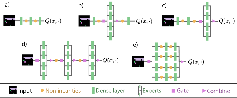
Figure 1: Architectures considered: (a) Baseline architecture; (b) Middle, used by Ceron et al. (2024b); (c) Final, where an MoE module replaces the final layer; (d) All, where all layers are replaced with an MoE module; (e) Big, with a single MoE module where an expert comprises the full original network.

2.2 MoEs

Mixtures of Experts (MoEs) emerged as a cornerstone in designing Large Language Models (LLMs), integrating a collection of $n$ “expert” sub-networks. A gating mechanism, known as the router and usually learned during training, manages the experts by directing each incoming token to $k$ selected experts (Shazeer et al., 2017). Typically, $k$ is less than the total count of experts (in our case, $k=1$). This sparsity is key for enhancing inference speed and facilitating distributed computing, making it a pivotal factor in training LLMs. In transformer architectures, MoE units substitute all dense feedforward layers (Vaswani et al., 2017). The impressive empirical performance of MoEs has sparked significant research interest (Shazeer et al., 2017; Lewis et al., 2021; Fedus et al., 2022; Zhou et al., 2022; Puigcerver et al., 2023; Lepikhin et al., 2020; Zoph et al., 2022; Gale et al., 2023).

The strict routing of tokens to specific experts, known as hard assignments, presents several issues, including training instability, token loss, and obstacles in expanding the number of experts (Fedus et al., 2022; Puigcerver et al., 2023). To mitigate these issues, Puigcerver et al. (2023) proposed the concept of Soft MoE, which utilises a soft, fully differentiable method for allocating tokens to experts, thereby circumventing the limitations associated with router-based hard assignments. This soft assignment method calculates a blend of weights for each token across the experts and aggregates their outputs accordingly. Adopting the terminology of Puigcerver et al. (2023), consider input tokens represented by $\mathbf{X}\in\mathbb{R}^{m\times d}$, with $m$ indicating the count of $d$-dimensional tokens. A Soft MoE layer processes these tokens through $n$ experts, each defined as $\{f_{i}:\mathbb{R}^{d}\rightarrow\mathbb{R}^{d}\}_{1:n}$. Every expert is associated with $p$ slots for both input and output, each slot characterised by a $d$-dimensional vector of parameters. These parameters are collectively denoted as $\boldsymbol{\Phi}\in\mathbb{R}^{d\times(n\cdot p)}$.

The input slots $\tilde{\mathbf{X}}\in\mathbb{R}^{(n\cdot p)\times d}$ represent a weighted average of all tokens, given by $\tilde{\mathbf{X}}=\mathbf{D}^{\top}\mathbf{X}$, where $\mathbf{D}$ is commonly known as the dispatch weights. The outputs from the experts are expressed as $\tilde{\mathbf{Y}}_{i}=f_{\lfloor i/p\rfloor}(\tilde{\mathbf{X}}_{i})$. For the Soft MoE layer, the overall output $\mathbf{Y}$ results from merging $\tilde{\mathbf{Y}}$ with the combined weights $\mathbf{C}$, described by $\mathbf{Y}=\mathbf{C}\tilde{\mathbf{Y}}$. $\mathbf{D}$ and $\mathbf{C}$ are represented by the following expressions:

$$\vphantom{\mathbf{C}_{ij}=\frac{\exp\left((\mathbf{X}\boldsymbol{\Phi})_{ij}\right)}{\sum_{j^{\prime}=1}^{n\cdot p}\exp\left((\mathbf{X}\boldsymbol{\Phi})_{ij^{\prime}}\right)}.}\mathbf{D}_{ij}=\frac{\exp\left((\mathbf{X}\boldsymbol{\Phi})_{ij}\right)}{\sum_{i^{\prime}=1}^{m}\exp\left((\mathbf{X}\boldsymbol{\Phi})_{i^{\prime}j}\right)}, \vphantom{\mathbf{D}_{ij}=\frac{\exp\left((\mathbf{X}\boldsymbol{\Phi})_{ij}\right)}{\sum_{i^{\prime}=1}^{m}\exp\left((\mathbf{X}\boldsymbol{\Phi})_{i^{\prime}j}\right)},}\mathbf{C}_{ij}=\frac{\exp\left((\mathbf{X}\boldsymbol{\Phi})_{ij}\right)}{\sum_{j^{\prime}=1}^{n\cdot p}\exp\left((\mathbf{X}\boldsymbol{\Phi})_{ij^{\prime}}\right)}.$$

The findings from Puigcerver et al. (2023) indicate that Soft MoE provides an improved balance between accuracy and computational expense relative to alternative MoE approaches.

3 Mixtures of Experts in a mixture of RL settings

Although shifting targets (due to bootstrapping) and dynamic data collection (from the agent’s policy) already render single-task RL a non-stationary problem, MTRL and CRL take this non-stationarity to an extreme by changing the environments during training. A critical difference between the two is that in MTRL, at every step, the agent interacts and learns from each environment (e.g. regular task-switching). In contrast, in CRL tasks are switched very infrequently. Thus, both settings provide complementary perspectives when investigating the efficacy of MoEs under high levels of non-stationarity.

3.1 Experimental setup

As we investigate many settings in many scenarios, we wanted to maximise the number of runs per setting to ensure statistical robustness, while keeping the computational expense at bay. For this reason, we chose to run our experiments with the PureJaxRL codebase (Lu et al., 2022b; a; 2023), which is a high-performance and parallelisable library including an implementation of Proximal Policy Optimisation (Schulman et al., 2017, PPO). Since Ceron et al. (2024b) focused on value-based methods, our use of PPO provides complementary insights and results. We rely on the Gymnax suite (Lange, 2022) to implement optimised versions of MinAtar environments (Young & Tian, 2019), which have been shown to provide insights comparable to the full ALE suite (Obando-Ceron & Castro, 2021). The hyper-parameters used are provided in Appendix H and were adapted from Jesson et al. (2023) (we deviate in the network size due to computational constraints). For all experiments, we evaluate on three environments: SpaceInvaders (SI), Breakout (BO), and Asterix (Ast). The input observations from Asterix differ substantially from SpaceInvaders and Breakout, whereas the latter are similar in observation and action space. This environment selection allows us to investigate whether MDP similarity encourages sharing representations between experts.

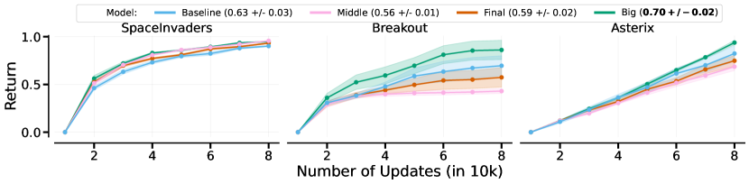
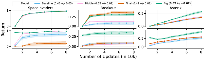
Figure 2: Measuring the impact of MoE architectures with hardcoded routing in MTRL (top). and CRL (bottom). In each legend, the numbers in parentheses indicate the average performance of each approach over all games. Big outperforms all other methods.

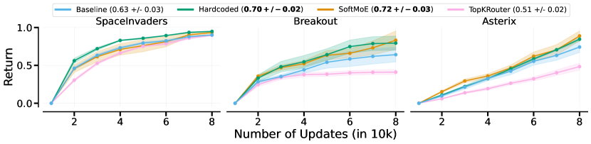
Figure 3: Measuring the impact of routing with Big architecture using different routing approaches under the MTRL (top row) and CRL (bottom row) settings. In each legend, the numbers in parentheses indicate the average performance of each approach across all games. SoftMoE and Hardcoded work best in MTRL, and Hardcoded works best in CRL, though SoftMoE still outperforms the baseline.

For MTRL we train simultaneously on SI, BO, and Ast; in practice, the PPO agent performs one update step per environment in sequence. For CRL, we train the agent on a fixed sequence of MDPs (Abbas et al., 2023) for $1e7$ environment steps ($\sim$ 80k update steps), specifically SI $\rightarrow$ BO $\rightarrow$ Ast $\rightarrow$ SI $\rightarrow$ BO $\rightarrow$ Ast. We present further analysis with different task orders in Section 4.

Ceron et al. (2024b) propose replacing the penultimate layer with an MoE module and sharing the other layers across the network. We term this variant Middle. We also evaluate a variant called Final, where the MoE module replaces the last layer. We also propose two new architectures: All, where MoE modules replace all three layers, and Big, where the network contains a single MoE module and each expert consists of a full network (see Figure 1). Since we are dealing with three distinct environments, all versions of MoEs have three experts. In all cases, we are using per-sample tokenization: one token – the state – per forward pass (Ceron et al., 2024b). All other hyper-parameters are reported in Appendix H.

We use a hardcoded routing strategy for many of our experiments to isolate the impact of routing versus expert architecture. This routing strategy will assign one expert for each task and route inputs accordingly. For the Big architecture, this effectively trains a separate network for each task and serves as a useful baseline. For all our results, we report the mean, averaged over $10$ independent seeds, with shaded areas representing standard error. In most figures, we also present the average normalised performance across all tasks (in parentheses in the legend), where normalisation scores were taken from Jesson et al. (2023). Our experiments were run on a single Tesla P$100$ or A$100$ GPU, each taking $10$ minutes. In total, we ran $870$ distinct settings over $10$ seeds each and are reported in Sections 3.2, 3.3, 4, A, B, C, D, E, F and G.

3.2 The impact of MoE architectures

To evaluate the impact of the choice of MoE architectures (Figure 1), we make use of the hardcoded router, which avoids potentially confounding factors due to also learning a routing strategy. In Figure 2, it is evident that the Big architecture performs best as expected since it is essentially a separate network per task. Still, it is promising to observe that all architectures outperform the baseline in the CRL setting, with All being the strongest performer. Surprisingly, in the MTRL setting, only Big outperforms the baseline. We hypothesise that All struggles due to suboptimal hyperparameters, as it was not computationally feasible to run a hyperparameter search over all possible settings. For Middle and Final, it is possible that gradient interference (Lyle et al., 2023) is complicating the learning process since there is parameter sharing outside of the MoE modules.

3.3 The impact of learned routers

The Big architecture provides a direct way to evaluate the impact of routing, as gating and combining are only done before and after the original network parameters, respectively. In Figure 3, we present the learning curves for Big architecture with varying routing strategies under CRL and MTRL.

In MTRL, we see little difference between the hardcoded router and SoftMoE. This is surprising since the hardcoded router trains separate networks for each task (performing as well as the baseline trained on each environment individually). This suggests that the gating used by SoftMoE is effective in situations where tasks are frequently changed. The rigidity of TopK routing appears to make it difficult for it to learn proper routing strategies, resulting in deteriorated performance.

In CRL, the hardcoded router performs best and retains previously learned policies (as evidenced by the second time the tasks are run). While SoftMoE ultimately outperforms the baseline in each task, it struggles in retaining previously learned policies; it is worth noting that the second time training on Ast, although its starting performance is essentially at zero, its final performance is higher than the first time training through, suggesting some policy retention (bottom right of Fig. 3).

A major learning challenge in the CRL setting is that no signal is provided to the network when the environment changes. Thus, a natural question is whether learned routers can effectively use task information. To investigate this, in Figure 4, we added the task ID as an input to the router (top row) and observed the surprising result that including task ID slightly hurts performance for Big-SoftMoE. Examining the gradient similarity from one update to the next (bottom left panel of Figure 4), it becomes evident that task-switching induces a discontinuity in the gradients used for learning. Interestingly, including this gradient similarity information as part of the input to the router does not hurt performance, but it does not improve either (bottom right).

In summary, our results suggest that SoftMoE routing is effective at dealing with high levels of non-stationarity, provided that discontinuous changes in environment dynamics (such as those arising from task switching) occur with relative frequency.

4 Extra Analyses

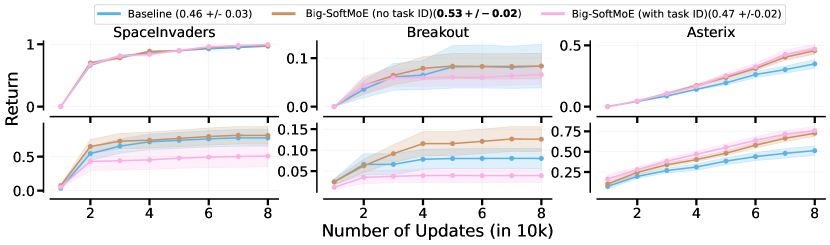
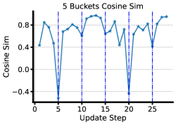
height 95pt depth 0 pt width 1.2 pt

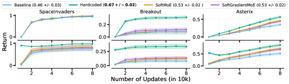
Figure 4: Top: Adding the task ID as an input to the router hurts performance for Big-SoftMoE. Bottom left: Sequential gradient similarity calculated throughout training, where dashed vertical lines represent when tasks switch. Bottom right: Adding gradient information as an input to the router does not improve performance.

In the previous section, we provided empirical evidence suggesting that MoEs can improve DRL agents’ performance in various non-stationary training regimes. Next, we conduct additional analyses to uncover the underlying causes of MoEs’ benefits.

Impact on network plasticity. We measure the fraction of dormant neurons (Sokar et al., 2023) during training as a proxy for network plasticity. As Figs. 5 (top), 11, and 15 demonstrate, all MoE variants reduce the fraction of dormant neurons, suggesting MoEs help with maintaining network plasticity, consistent with the findings of Ceron et al. (2024b).

Expert specialisation. In Figs. 5 (bottom), 10, and 16 we measure the probabilities assigned to each expert during training; what these values indicate is the likelihood that inputs will be routed to each respective expert; observe that the hardcoded router has maximal specialisation, where each expert is assigned to one task. We can also observe that both Big-SoftMoE and All-SoftMoE variants tend to specialise in all layers.

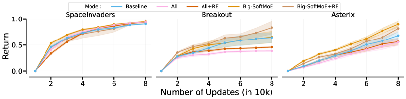
Figure 14: MTRL: Regularising the entropy does not affect performance significantly, suggesting that specialisation only plays a limited role for performance.

In supervised learning settings, it is common to use load-balancing losses to avoid this type of specialisation to maximise expert usage. We explored this idea by adding entropy regularisation during training and observed that, while we do see a decrease in expert specialisation (c.f. Figs. 4 (bottom), 10, and 16), this does not affect performance in any meaningful way (c.f. Figs. 14 and 8).

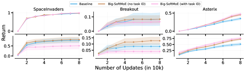
Figure 9: CRL: Adding Task ID as input slightly hurts performance for Big-SoftMoE.

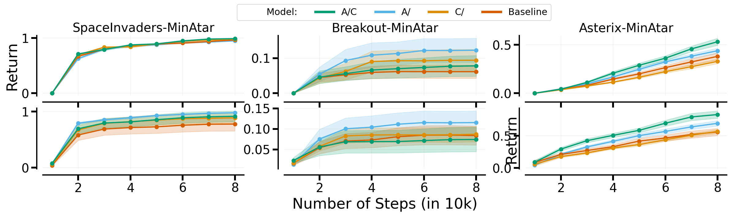
Figure 17: CRL: In general, having an MoE module in the actor seems to be most helpful for performance, whereas the critic MoE module does not improve performance significantly. We used the Big variant for the ablation.

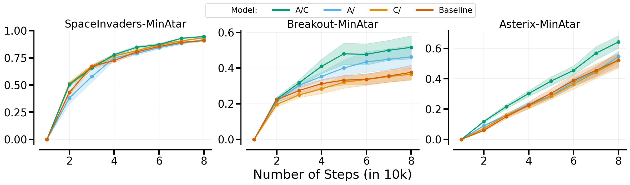
Figure 18: MTRL: The combination of Actor and Critic MoE modules appears most beneficial. We used the Big variant for the ablation.

Impact on actor and critic networks. Ceron et al. (2024b) focused on value-based methods (where a single network serves as critic and actor), so using an actor-critic method like PPO provides a novel, complementary perspective. By default, we use MoE modules on the actor and critic networks, but in Figs. 6, 17, 18, 9 and 10, we show that, in the two settings, it is best to use MoEs on both networks. However, the results suggest that MoEs have a greater impact on the actor than on the critic network. The fact that actor networks seem to benefit more from MoEs than critic networks is aligned with the findings of Graesser et al. (2022), where they found that actor networks could handle much higher levels of sparsity than critics without any degradation in performance.

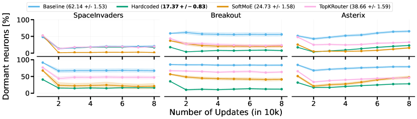
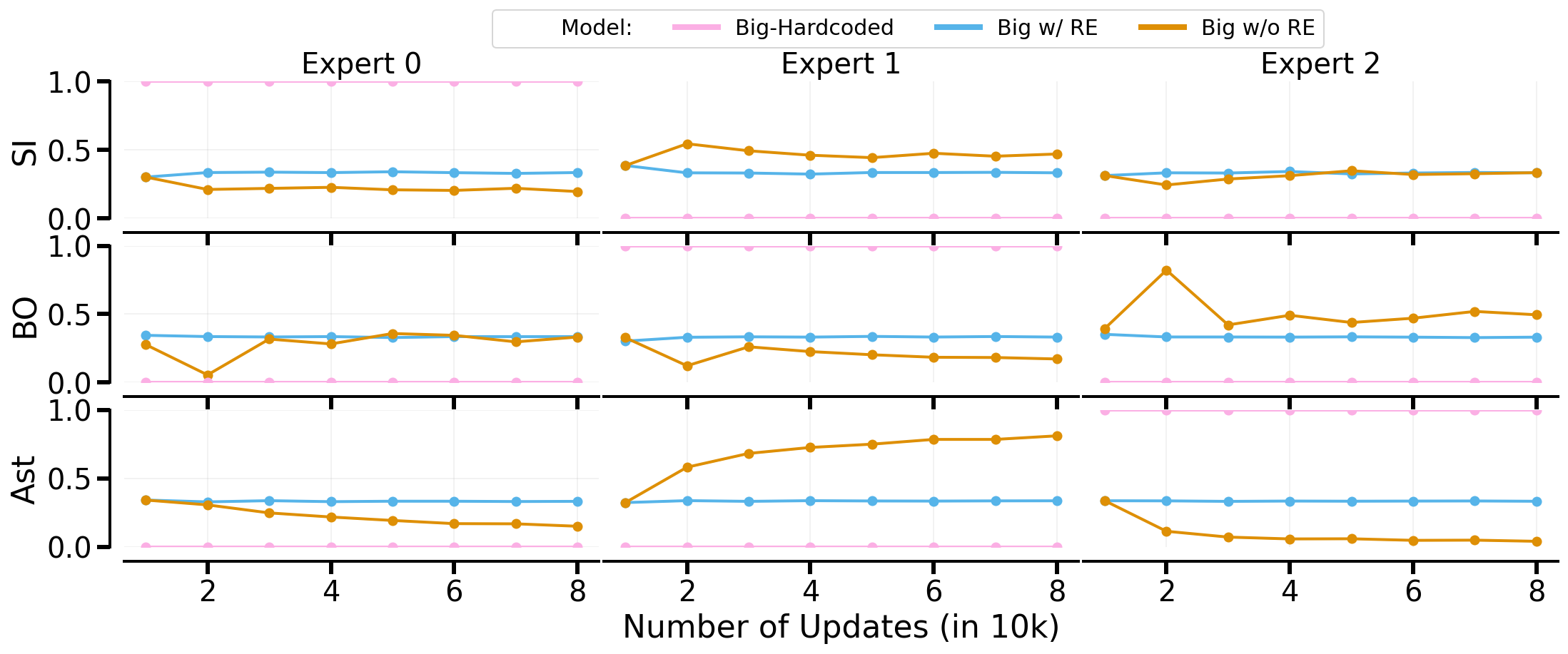
Figure 5: Top: presents the ratio of dormant neurons for CRL under different routing approaches using Big. The numbers in the legend represent average dormant neuron fractions across all games. MoE variants have lower dormant neurons than the baseline. Bottom: Regularising the entropy of the router makes the expert selection more uniform. Without regularisation, there is more specialisation. This shows one seed, as different seeds might choose different experts. See section 4 for more details.

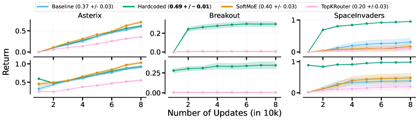
Figure 20: CRL: The order does affect the conclusion for CRL, especially because Breakout performance completely collapses if trained first on Asterix, then Breakout, then SpaceInvaders. Learned routers now do not perform better than the baseline. Big-Hardcoded still works as expected.

Order of environments. To investigate the impact of environment ordering, we train using the ordering Ast $\rightarrow$ BO $\rightarrow$ SI to compare with the orderings we have used thus far; we present results for MTRL and CRL in Figs. 20 and 21, respectively. While conclusions do not change in MTRL, changing the order of environments affects CRL performance significantly (excluding the hardcoded router). We observe two interesting changes: (i) training BO after Ast (as opposed to after SI) causes all methods (excluding hardcoded) to collapse, and (ii) when training on Ast last, none of the agents were able to retain the learned policy (c.f. Fig. 3), whereas when training on Ast first there is some policy retention (as seen on the bottom left of Fig. 20). As mentioned previously, Ast differs substantially from the other two environments, so our findings in Fig. 20 suggest that the agents have overfit the input distribution of Ast, hindering its ability to adapt to the other environments but allowing the retention of the policy learned on Ast.

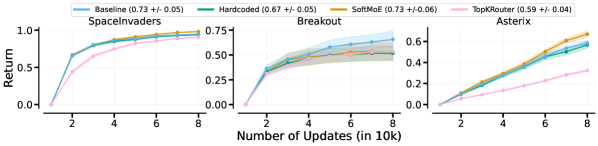
Figure 30: Left: Aggregate Interquantile Mean (Agarwal et al., 2021) of scores. Right Comparison of different models and routers on the single environment setup. We report the mean of the normalised scores for 3 Atari games. All games run with 10 independent seeds, shaded areas representing the standard error. We normalise performance according to the single environment results reported in Jesson et al. (2023). BigMoE improves performance over the baseline, especially due to performance improvements in Asterix.

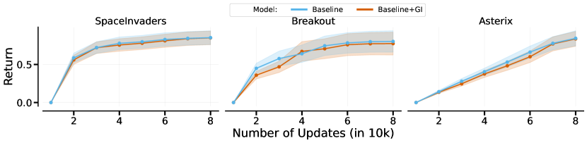
Figure 34: Single environment: Baseline vs. Baseline with Gradient Information, adding gradient information to the input of the baseline does not affect its performance.

Single Environment. Despite the clear improvements from CRL and MTRL, there are no significant performance improvements across all games in the single environment setting. However, Big improves over the baseline in Asterix while performing worse in Breakout, as shown in Figure 30 and Table 21, suggesting that MoEs might be beneficial in specific types of environments. Adding gradient information did not affect performance (see Figure 34).

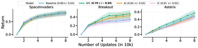
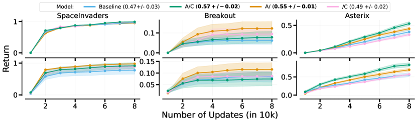
Figure 6: Comparing the impact of MoE architectures on actor and critic networks with the hardcoded router, under the MTRL (top row) and CRL (bottom row) settings. In each legend, the numbers in parentheses indicate the average performance of each approach across all games. It is best to use MoEs on both networks. However, the results suggest that MoEs have a greater impact when used on the actor network than on the critic. See section 4 for more details.

5 Related Work

Parameter underutilisation is a roadblock to parameter efficiency in deep Reinforcement Learning (RL). The latter was highlighted by Sokar et al. (2023) in the form of dormant neurons. Arnob et al. (2021) demonstrate that in offline RL, up to 95% of network parameters can be pruned at initialisation without impacting performance. Further, several studies have shown that periodic network weight resets enhance performance (Igl et al., 2020; Dohare et al., 2021; Nikishin et al., 2022b; D’Oro et al., 2022; Sokar et al., 2023; Schwarzer et al., 2023) and that RL networks maintain performance when trained with a high degree of sparsity (Tan et al., 2022; Sokar et al., 2022; Graesser et al., 2022; Ceron et al., 2024a). These findings underscore the need for methods that more effectively leverage network parameters in RL training. Our work explores the use of Mixture of Experts (MoEs) for actor-critic methods, demonstrating significant reductions in dormant neurons across various tasks and network architectures.

Mixtures of Experts (MoEs) revolutionised large-scale language/vision models primarily due to their modular design, which supports distributed training and enhances parameter efficiency during inference (Lepikhin et al., 2020; Fedus et al., 2022; Yang et al., 2019; Wang et al., 2020; Abbas & Andreopoulos, 2020; Pavlitskaya et al., 2020). MoEs show benefits in transfer and multi-task learning scenarios, e.g., by assigning experts to specific sub-problems (Puigcerver et al., 2023; Chen et al., 2023; Ye & Xu, 2023), or by improving the statistical performance of routers (Hazimeh et al., 2021).

MoEs have been studied in DRL (Ren et al., 2021; Hendawy et al., 2024; Akrour et al., 2021) but based on a previous definition of MoE (Jacobs et al., 1991), closely related to ensembling, and not the more recent interpretation of MoEs in LLMs. Ensembles are often used to represent the policy (Anschel et al., 2016; Lan et al., 2020; Agarwal et al., 2020; Peer et al., 2021; Chen et al., 2021; An et al., 2021; Wu et al., 2021; Liang et al., 2022) or to predict model dynamics (Shyam et al., 2019; Chua et al., 2018; Kurutach et al., 2018). Most closely related to ensembling is our Big architecture, where each expert is a full model. Fan et al. (2023) could be interpreted as using multiple meta-controllers as routers for Big and ensembling the resulting policy. In contrast to our work, they do not investigate different MoE architectures and rely on population-based training.

Two recent works have explored using MoEs (as used in LLMs) in DRL: the work of Ceron et al. (2024b) has already been referenced extensively above, as our work builds on their findings. More recently, Farebrother et al. (2024) argued that classification losses yield stabler learning dynamics than regression losses, which also applies to using MoEs.

6 Conclusion

Our work provides additional evidence of the effectiveness of MoEs in improving the training of DRL agents. Using MTRL and CRL grants us a novel perspective on evaluating and analysing MoEs under “extreme” non-stationarity. Consistent with the findings of Ceron et al. (2024b), DRL is most performant using SoftMoE, whereas it struggles with hard TopK routing.

Our use of the hardcoded router served as a useful baseline for our analyses and demonstrates much room for improvement in training DRL agents in multi-task settings. Indeed, in CRL, only mild policy retention was observed in Ast, and the retention amount was dependent on the order in which the environments were trained. An exciting avenue for future work is thus investigating what task curricula would lead to best agent performance and policy retention. As mentioned previously, the observations in Ast differ substantially from those of BO and SI (which are similar to each other); the fact that we only observed policy retention in Ast thus begs the question of whether the agent is over-fitting to the anomalous input distribution of Ast, at the expense of being able to generalise to the other environments.

Expert specialisation and whether load-balancing is desirable are also interesting questions for future research. The findings from the supervised learning community in this respect may not naturally carry over to DRL settings, largely due to training’s inherent non-stationarity. Finally, MoEs could be investigated in multi-agent settings, where experts represent different agents in cooperative (Ellis et al., 2024) or general-sum settings (Lu et al., 2022b; Willi et al., 2022), where vectorised environments are widely available (Khan et al., 2023; Rutherford et al., 2023).

Acknowledgements

The authors would like to thank Gheorghe Comanici, Gopeshh Subbaraj, Doina Precup, Hugo Larochelle, and the rest of the Google DeepMind Montreal team for valuable discussions during the preparation of this work. Gheorghe Comanici deserves a special mention for providing us valuable feed-back on an early draft of the paper. We thank the anonymous reviewers for their valuable help in improving our manuscript. We would also like to thank the Python community Van Rossum & Drake Jr (1995); Oliphant (2007) for developing tools that enabled this work, including NumPy Harris et al. (2020), Matplotlib Hunter (2007), Jupyter Kluyver et al. (2016), Pandas McKinney (2013) and JAX Bradbury et al. (2018).

Broader Impact Statement

This paper introduces research aimed at pushing the boundaries of Machine Learning, with a particular focus on reinforcement learning. Our work holds various potential societal implications, although we refrain from singling out specific ones for emphasis in this context.

Appendix A Continual RL

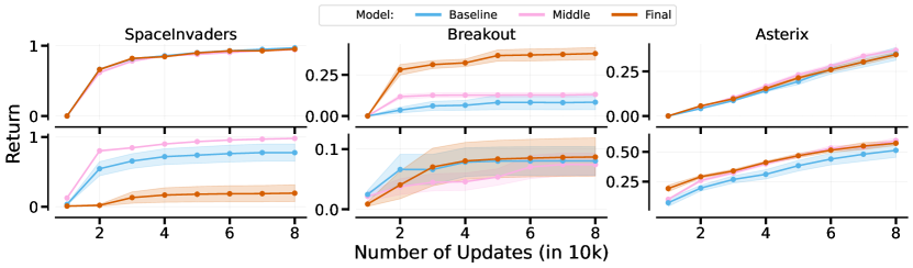
Figure 7: CRL: Variants with shared parameters across task do not necessarily improve performance over the baseline. Middle performs better than the baseline, whereas Final does not.

Game	Baseline	Final-Hardcoded	Middle-Hardcoded
SI	$0.97\pm 0.01$	$0.95\pm 0.01$	$0.94\pm 0.01$
BO	$0.08\pm 0.05$	$0.38\pm 0.04$	$0.13\pm 0.01$
Ast	$0.35\pm 0.04$	$0.34\pm 0.01$	$0.37\pm 0.01$
SI-2	$0.78\pm 0.12$	$0.19\pm 0.12$	$0.98\pm 0.01$
BO-2	$0.08\pm 0.02$	$0.09\pm 0.03$	$0.07\pm 0.02$
Ast-2	$0.51\pm 0.06$	$0.57\pm 0.02$	$0.60\pm 0.02$
Total	$0.46\pm 0.03$	$0.42\pm 0.02$	$\textbf{0.52}\pm\textbf{0.01}$

Table 1: CRL: Variants with shared parameters across task do not necessarily improve performance over the baseline. Middle performs better than the baseline, whereas Final does not.

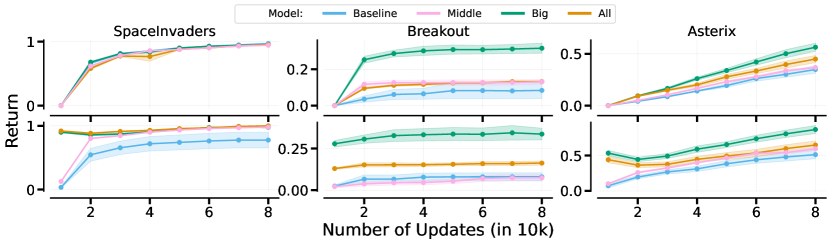
Figure 8: CRL: Isolated Params: Variants with isolated parameters across task improve performance over the baseline. Big-Hardcoded works the best.

Game	Baseline	All-Hardcoded	Big-Hardcoded	Middle-Hardcoded
Game	Baseline	Final-Hardcoded	Middle-Hardcoded	Additional-Column
SI	$0.97\pm 0.01$	$0.95\pm 0.01$	$0.95\pm 0.00$	$0.94\pm 0.01$
BO	$0.08\pm 0.05$	$0.13\pm 0.00$	$0.32\pm 0.03$	$0.13\pm 0.01$
Ast	$0.35\pm 0.04$	$0.45\pm 0.03$	$0.56\pm 0.04$	$0.37\pm 0.01$
SI-2	$0.78\pm 0.12$	$1.00\pm 0.00$	$0.98\pm 0.01$	$0.98\pm 0.01$
BO-2	$0.08\pm 0.02$	$0.16\pm 0.01$	$0.34\pm 0.04$	$0.07\pm 0.02$
Ast-2	$0.51\pm 0.06$	$0.65\pm 0.06$	$0.87\pm 0.06$	$0.60\pm 0.02$
Total	$0.46\pm 0.03$	$0.56\pm 0.02$	$\textbf{0.67}\pm\textbf{0.02}$	$0.52\pm 0.01$

Table 2: CRL: Isolated Params: Variants with isolated parameters across task improve performance over the baseline. Big-Hardcoded works the best.

Game	Baseline	w/ Task-ID	w/o Task-ID
SI	$0.97\pm 0.01$	$0.98\pm 0.01$	$0.99\pm 0.01$
BO	$0.08\pm 0.05$	$0.08\pm 0.03$	$0.07\pm 0.02$
Ast	$0.35\pm 0.04$	$0.46\pm 0.03$	$0.47\pm 0.04$
SI-2	$0.78\pm 0.12$	$0.81\pm 0.13$	$0.51\pm 0.16$
BO-2	$0.08\pm 0.02$	$0.13\pm 0.03$	$0.04\pm 0.02$
Ast-2	$0.51\pm 0.06$	$0.73\pm 0.04$	$0.76\pm 0.05$
Total	$0.46\pm 0.03$	$\textbf{0.53}\pm\textbf{0.02}$	$0.47\pm 0.02$

Table 3: CRL: Adding Task ID as input slightly hurts performance for Big-SoftMoE.

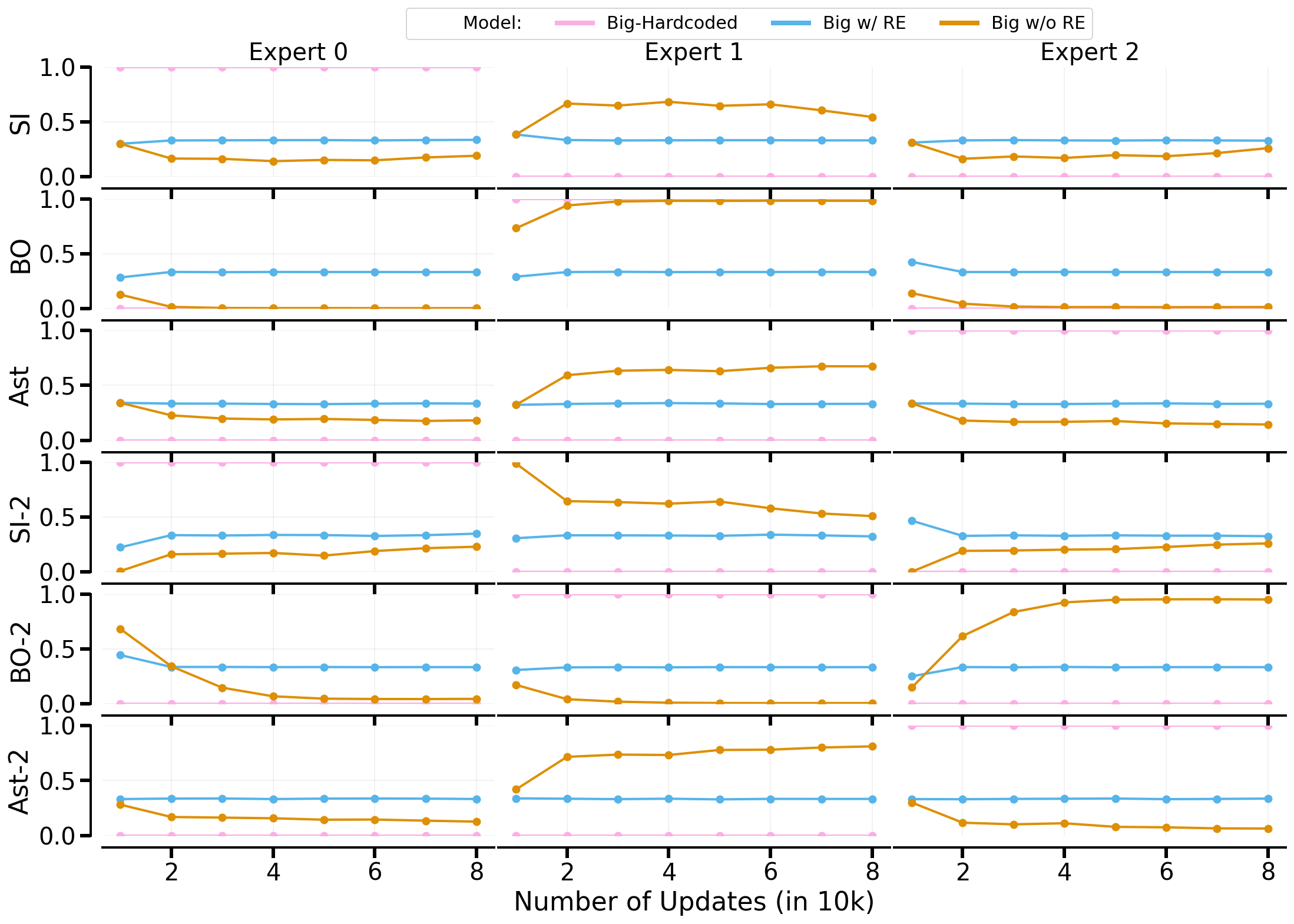
Figure 10: CRL: Big-SoftMoE also specialises in the CRL setting.

Game	Baseline	Big-Hardcoded	Big-SoftGradMoE	Big-SoftMoE
SI	$0.97\pm 0.01$	$0.95\pm 0.00$	$0.99\pm 0.01$	$0.98\pm 0.01$
BO	$0.08\pm 0.05$	$0.32\pm 0.03$	$0.12\pm 0.03$	$0.08\pm 0.03$
Ast	$0.35\pm 0.04$	$0.56\pm 0.04$	$0.45\pm 0.04$	$0.46\pm 0.03$
SI-2	$0.78\pm 0.12$	$0.98\pm 0.01$	$0.79\pm 0.13$	$0.81\pm 0.13$
BO-2	$0.08\pm 0.02$	$0.34\pm 0.04$	$0.14\pm 0.03$	$0.13\pm 0.03$
Ast-2	$0.51\pm 0.06$	$0.87\pm 0.06$	$0.69\pm 0.06$	$0.73\pm 0.04$
Total	$0.46\pm 0.03$	$\textbf{0.67}\pm\textbf{0.02}$	$0.53\pm 0.02$	$0.53\pm 0.02$

Table 4: Performance of algorithms across games with total performance.

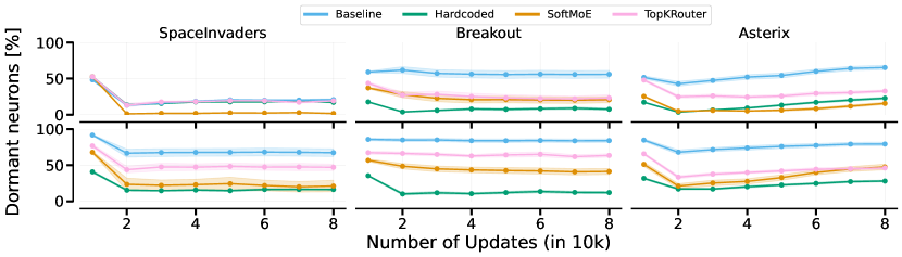
Figure 11: CRL: MoE variants have less dormant neurons than the baseline without MoE modules.

Game	Baseline	Big-Hardcoded	Big-TopK	Big-SoftMoE
SI	$20.86\pm 1.41$	$17.19\pm 0.94$	$19.22\pm 1.78$	$1.72\pm 0.45$
BO	$55.94\pm 5.38$	$7.58\pm 1.44$	$23.20\pm 4.71$	$20.86\pm 4.34$
Ast	$65.31\pm 3.13$	$22.89\pm 1.49$	$32.73\pm 1.72$	$15.70\pm 1.65$
SI-2	$67.34\pm 5.38$	$16.41\pm 1.22$	$47.11\pm 4.49$	$21.17\pm 7.97$
BO-2	$84.06\pm 2.41$	$12.11\pm 1.61$	$63.52\pm 2.47$	$41.33\pm 4.19$
Ast-2	$79.30\pm 2.65$	$28.05\pm 1.27$	$46.17\pm 1.76$	$47.58\pm 3.94$
Total	$62.14\pm 1.53$	$\textbf{17.37}\pm\textbf{0.83}$	$38.66\pm 1.59$	$24.73\pm 1.58$

Table 5: CRL Dormant Neurons for Big router variants. The hardcoded variant has the least dormant neurons

A.1 Hard-switching based on Gradient Similarity

We also attempt to route when the gradient similarity drops below a threshold. However, this proved difficult as the thresholds depend on the architecture and expert might switch too early, as shown in Figure 12.

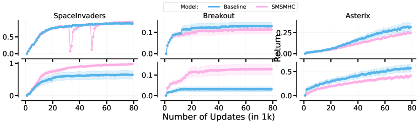
Figure 12: CRL: As shown here with SMSMHC, finding a correct threshold for gradient switching proves difficult, as the experts might switch too early, as in this case it already switches twice during SpaceInvaders (see the dips)

Game	Baseline	Big-Hardcoded	Big-TopK	Big-SoftMoE
SI	$21.95\pm 1.15$	$22.34\pm 1.12$	$19.61\pm 2.10$	$2.89\pm 0.40$
BO	$22.50\pm 3.02$	$7.89\pm 1.21$	$20.39\pm 1.36$	$3.91\pm 1.23$
Ast	$72.66\pm 1.59$	$29.14\pm 1.11$	$44.30\pm 2.35$	$26.02\pm 1.21$
Total	$39.04\pm 0.88$	$19.79\pm 0.92$	$28.10\pm 1.81$	$\textbf{10.94}\pm\textbf{0.77}$

Table 6: MTRL Dormant Neurons for Big router variants. Big-SoftMoE has the least dormant neurons.

Appendix B Multi-Task RL

Combining router learning with some task-specialized layers via Hardcoding.

We perform preliminary tests how enforced task-specialization in the final layer affects performance. For this, we introduce a new architecture termed SMSMHC (SoftMoE, SoftMoE, Hardcoded Router). This architecture consists of two initial layers of learned SoftMoE and a final layer with a Hardcoded Router. Contrary to expectations, SMSMHC does not yield a performance improvement (0.56 $\pm$ 0.02 and 0.53 $\pm$ 0.01), as shown in Figure 13, leading to questions about the value of specialization in this context.

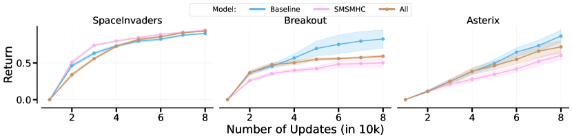
Figure 13: MTRL: SMSMHC does not improve performance over All, suggesting that extreme specialisation in the last layer is not necessarily helpful.

Game	Baseline	All	SMSMHC
SI	$0.90\pm 0.01$	$0.94\pm 0.01$	$0.95\pm 0.00$
BO	$0.46\pm 0.07$	$0.33\pm 0.01$	$0.28\pm 0.03$
Ast	$0.51\pm 0.05$	$0.43\pm 0.05$	$0.36\pm 0.04$
Total	$\textbf{0.63}\pm\textbf{0.03}$	$0.56\pm 0.02$	$0.53\pm 0.01$

Table 7: MTRL: SMSMHC does not improve performance over All, suggesting that extreme specialisation in the last layer is not necessarily helpful.

Game	Baseline	All w/o RE	All w/ RE	Big w/o RE	Big w/ RE
SI	$0.90\pm 0.01$	$0.94\pm 0.01$	$0.94\pm 0.01$	$0.95\pm 0.01$	$0.93\pm 0.01$
BO	$0.46\pm 0.07$	$0.28\pm 0.01$	$0.33\pm 0.01$	$0.47\pm 0.08$	$0.60\pm 0.09$
Ast	$0.51\pm 0.05$	$0.42\pm 0.05$	$0.43\pm 0.05$	$0.68\pm 0.04$	$0.62\pm 0.05$
Total	$0.63\pm 0.03$	$0.55\pm 0.02$	$0.56\pm 0.02$	$\textbf{0.70}\pm\textbf{0.02}$	$\textbf{0.72}\pm\textbf{0.03}$

Table 8: MTRL: Regularising the entropy does not affect performance significantly, suggesting that specialisation only plays a limited role for performance.

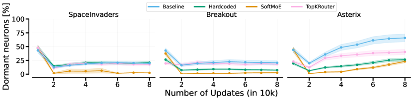
Figure 15: MTRL: Generally, dormant neurons are lower when using Big variants.

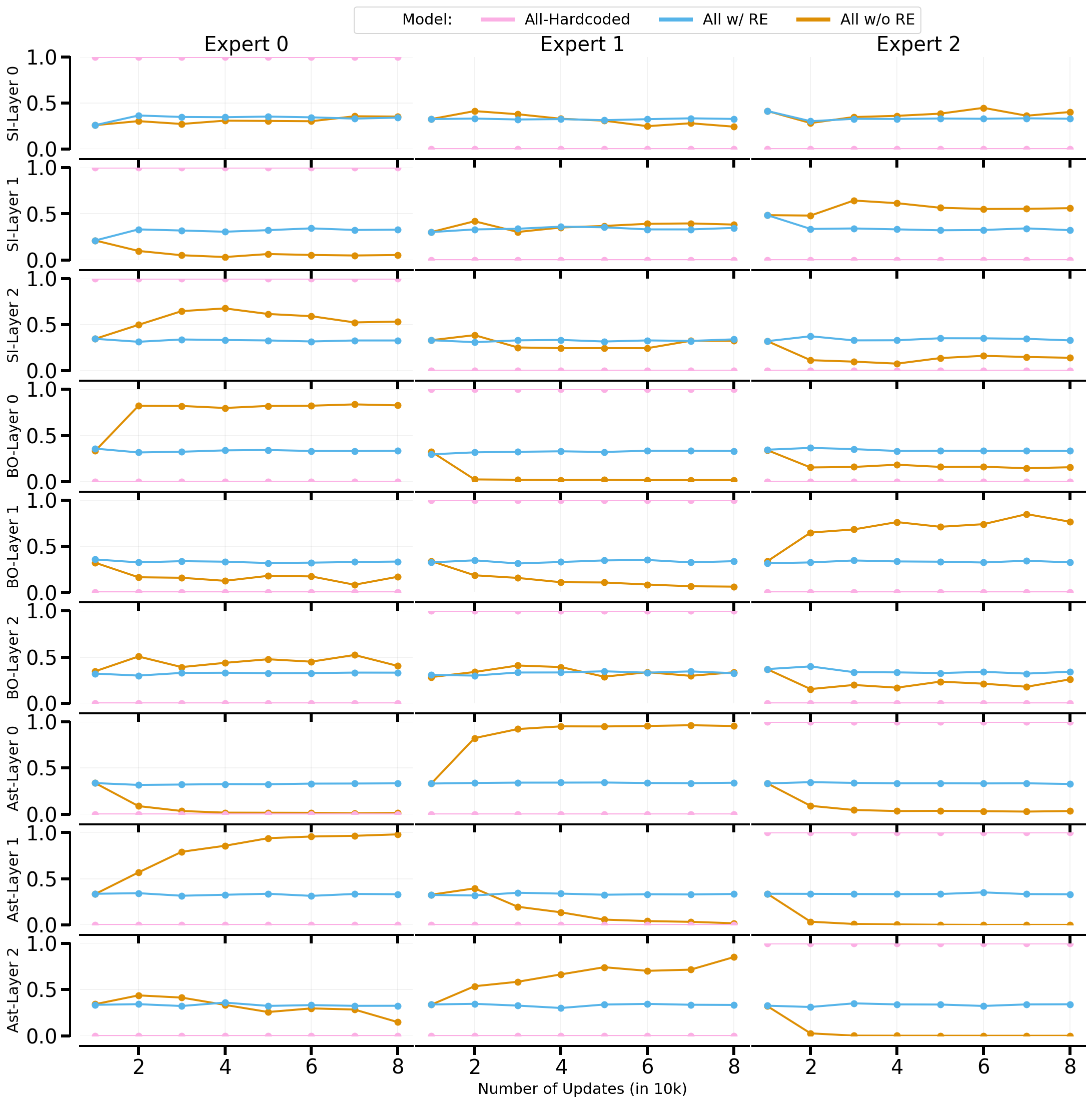
Figure 16: MTRL: Row 1-3 is Layer 1-3 when playing SpaveInvaders, row 4-6, is layer 1-3 when playing Breakout, row 7-9 is layer 1-3 when playing Asterix.

Appendix C Actor/Critic Ablation

Game	Baseline	/C	A/	A/C
SI	$0.96\pm 0.00$	$0.98\pm 0.01$	$0.95\pm 0.01$	$0.99\pm 0.01$
BO	$0.06\pm 0.02$	$0.09\pm 0.03$	$0.12\pm 0.03$	$0.08\pm 0.03$
Ast	$0.38\pm 0.04$	$0.33\pm 0.02$	$0.44\pm 0.03$	$0.53\pm 0.04$
SI-2	$0.78\pm 0.12$	$0.88\pm 0.09$	$0.97\pm 0.01$	$0.91\pm 0.10$
BO-2	$0.08\pm 0.02$	$0.09\pm 0.02$	$0.12\pm 0.03$	$0.07\pm 0.03$
Ast-2	$0.56\pm 0.06$	$0.56\pm 0.03$	$0.71\pm 0.05$	$0.81\pm 0.05$

Table 9: CRL: In general, having an MoE module in the actor seems to be most helpful for performance, whereas the critic MoE module does not improve performance significantly. We used the Big variant for the ablation.

Game	Baseline	/C	A/	A/C
SI	$0.91\pm 0.01$	$0.93\pm 0.01$	$0.92\pm 0.00$	$0.95\pm 0.01$
BO	$0.38\pm 0.04$	$0.37\pm 0.03$	$0.46\pm 0.06$	$0.52\pm 0.07$
Ast	$0.52\pm 0.04$	$0.52\pm 0.05$	$0.55\pm 0.04$	$0.64\pm 0.04$
Total	$0.60\pm 0.02$	$0.61\pm 0.02$	$0.64\pm 0.02$	$\mathbf{0.70\pm 0.03}$

Table 10: MTRL: The combination of Actor and Critic MoE modules appears most beneficial. We used the Big variant for the ablation.

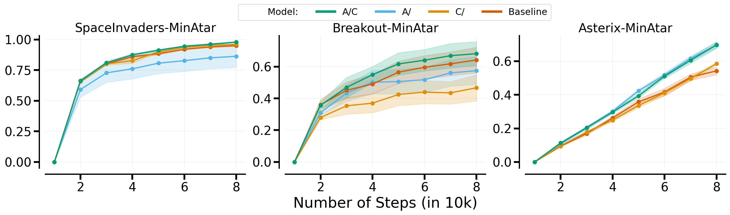
Figure 19: There is no significant difference in using either Actor or Critic, though the combination of both works significantly better than using only the Critic.

Game	Baseline	A/C	A/	C/
SI	$0.95\pm 0.01$	$0.98\pm 0.00$	$0.86\pm 0.09$	$0.96\pm 0.00$
BO	$0.64\pm 0.08$	$0.68\pm 0.08$	$0.57\pm 0.09$	$0.47\pm 0.08$
Ast	$0.54\pm 0.02$	$0.70\pm 0.02$	$0.70\pm 0.02$	$0.59\pm 0.01$
Total	$\mathbf{0.71\pm 0.05}$	$\mathbf{0.79\pm 0.05}$	$\mathbf{0.71\pm 0.07}$	$0.67\pm 0.05$

Table 11: There is no significant difference in using either Actor or Critic, though the combination of both works significantly better than using only the Critic.

Appendix D Order Ablation

Game	Baseline	Big-Hardcoded	Big-TopK	Big-SoftMoE
SI	$0.31\pm 0.13$	$0.95\pm 0.01$	$0.10\pm 0.08$	$0.17\pm 0.10$
BO	$0.01\pm 0.00$	$0.30\pm 0.03$	$0.01\pm 0.00$	$0.01\pm 0.00$
Ast	$0.60\pm 0.02$	$0.61\pm 0.02$	$0.35\pm 0.02$	$0.70\pm 0.02$
SI-2	$0.38\pm 0.14$	$0.98\pm 0.01$	$0.20\pm 0.11$	$0.48\pm 0.15$
BO-2	$0.01\pm 0.00$	$0.34\pm 0.04$	$0.01\pm 0.00$	$0.01\pm 0.00$
Ast-2	$0.91\pm 0.03$	$0.93\pm 0.03$	$0.55\pm 0.02$	$1.04\pm 0.03$
Total	$0.37\pm 0.03$	$\mathbf{0.69\pm 0.01}$	$0.20\pm 0.03$	$0.40\pm 0.03$

Table 12: CRL: The order does affect the conclusion for CRL, especially because Breakout performance completely collapses if trained first on Asterix, then Breakout, then SpaceInvaders. Learned routers now do not perform better than the baseline. Big-Hardcoded still works as expected.

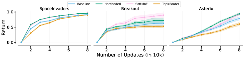
Figure 21: MTRL: The conclusions do not change when changing the order of training for MTRL. Learned routers and hardcoded routers perform on par and better than the baseline.

Game	Baseline	Big-Hardcoded	Big-TopK	Big-SoftMOE
SI	$0.92\pm 0.01$	$0.95\pm 0.00$	$0.90\pm 0.01$	$0.97\pm 0.00$
BO	$0.34\pm 0.05$	$0.39\pm 0.05$	$0.29\pm 0.02$	$0.49\pm 0.04$
Ast	$0.51\pm 0.04$	$0.61\pm 0.02$	$0.39\pm 0.04$	$0.60\pm 0.03$
Total	$0.59\pm 0.02$	$0.65\pm 0.02$	$0.53\pm 0.01$	$0.68\pm 0.02$

Table 13: MTRL: The conclusions do not change when changing the order of training for MTRL. Learned routers and hardcoded routers perform on par and better than the baseline.

Appendix E MTRL - More Results

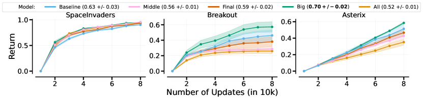
Figure 22: MTRL: All Hardcoded architectures, Big-Hardcoded works best. It is unclear why All does not perform as well as Big, though we hypothesise it is due to suboptimal hyperparameters

Game	Baseline	All	Big	Final	Middle
SI	$0.90\pm 0.01$	$0.94\pm 0.01$	$0.95\pm 0.01$	$0.93\pm 0.01$	$0.96\pm 0.01$
BO	$0.46\pm 0.07$	$0.26\pm 0.03$	$0.57\pm 0.07$	$0.38\pm 0.07$	$0.29\pm 0.02$
Ast	$0.51\pm 0.05$	$0.35\pm 0.04$	$0.59\pm 0.01$	$0.47\pm 0.03$	$0.43\pm 0.03$
Total	$0.63\pm 0.03$	$0.52\pm 0.01$	$0.70\pm 0.02$	$0.59\pm 0.02$	$0.56\pm 0.01$

Table 14: MTRL: All Hardcoded architectures: Big-Hardcoded works best. It is unclear why All does not perform as well as Big, though we hypothesise it is due to suboptimal hyperparameters.

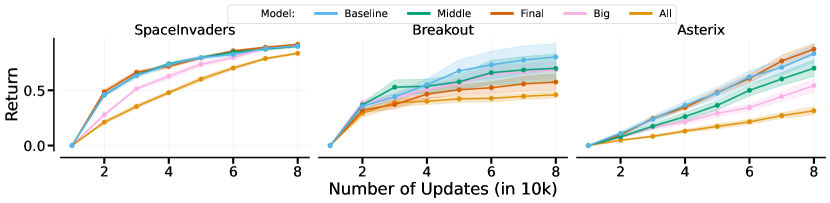
Figure 23: MTRL: All TopKRouter architectures: Generally, TopKRouters perform worse than the baseline.

Game	Baseline	All	Big	Final	Middle
SI	$0.90\pm 0.01$	$0.83\pm 0.01$	$0.91\pm 0.01$	$0.92\pm 0.00$	$0.90\pm 0.01$
BO	$0.46\pm 0.07$	$0.27\pm 0.02$	$0.40\pm 0.04$	$0.33\pm 0.04$	$0.40\pm 0.07$
Ast	$0.51\pm 0.05$	$0.19\pm 0.02$	$0.34\pm 0.03$	$0.54\pm 0.03$	$0.43\pm 0.05$
Total	$\mathbf{0.63\pm 0.03}$	$0.43\pm 0.01$	$0.55\pm 0.02$	$\mathbf{0.60\pm 0.01}$	$\mathbf{0.58\pm 0.03}$

Table 15: MTRL: All TopKRouter architectures: Generally, TopKRouters perform worse than the baseline.

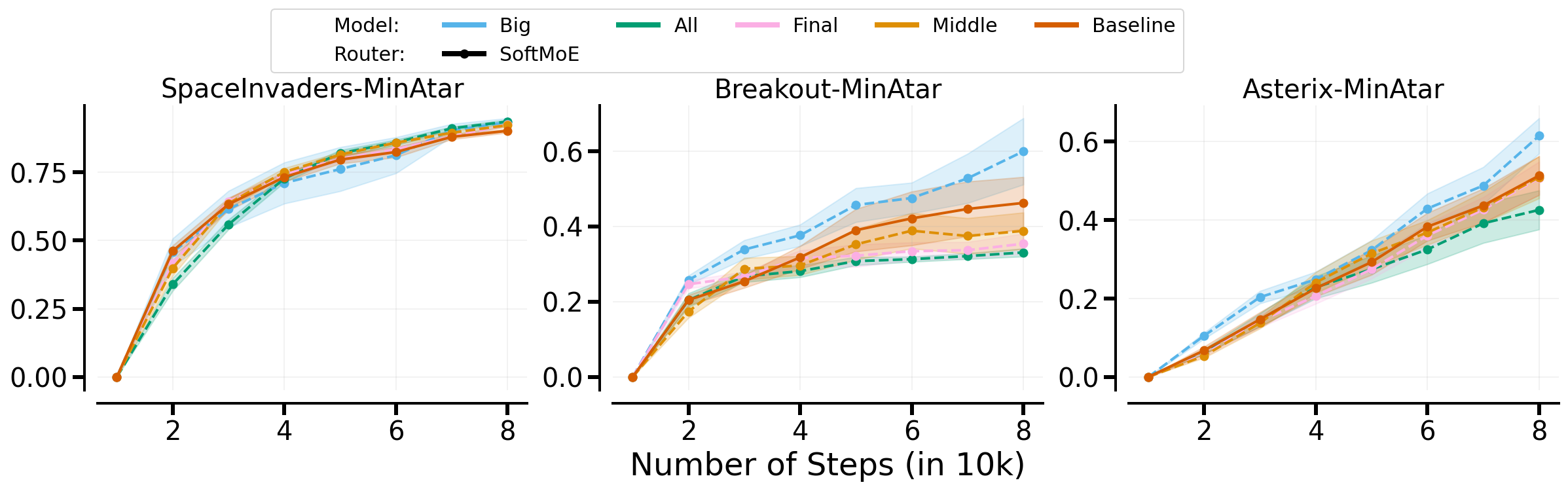
Figure 24: MTRL: All SoftMoE Architectures: Only Big-SoftMoE performs better than the baseline.

Game	Baseline	All	Big	Final	Middle
SI	$0.90\pm 0.01$	$0.94\pm 0.01$	$0.93\pm 0.01$	$0.92\pm 0.01$	$0.92\pm 0.01$
BO	$0.46\pm 0.07$	$0.33\pm 0.01$	$0.60\pm 0.09$	$0.35\pm 0.03$	$0.39\pm 0.05$
Ast	$0.51\pm 0.05$	$0.43\pm 0.05$	$0.62\pm 0.05$	$0.51\pm 0.04$	$0.51\pm 0.05$
Total	$0.63\pm 0.03$	$0.56\pm 0.02$	$\mathbf{0.72\pm 0.03}$	$0.60\pm 0.02$	$0.61\pm 0.02$

Table 16: MTRL: All SoftMoE Architectures: Only Big-SoftMoE performs better than the baseline.

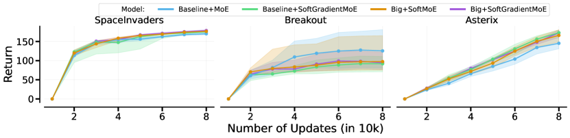
Figure 25: MTRL: Big-SoftGradientMoE vs. Big-SoftMoE, adding gradient information does not improve performance.

Game	Baseline	Big-Hardcoded	Big-SoftGradientMoE	Big-SoftMoE
SI	$0.90\pm 0.01$	$0.95\pm 0.01$	$0.95\pm 0.00$	$0.93\pm 0.01$
BO	$0.46\pm 0.07$	$0.57\pm 0.07$	$0.51\pm 0.07$	$0.60\pm 0.09$
Ast	$0.51\pm 0.05$	$0.59\pm 0.01$	$0.66\pm 0.03$	$0.62\pm 0.05$
Total	$0.63\pm 0.03$	$\mathbf{0.70\pm 0.02}$	$\mathbf{0.70\pm 0.03}$	$\mathbf{0.72\pm 0.03}$

Table 17: MTRL: Big-SoftGradientMoE vs. Big-SoftMoE, adding gradient information does not improve performance.

Appendix F CRL - More Results

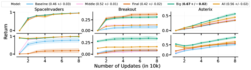
Figure 26: CRL: All HardcodedRouter Architectures. Big-Hardcoded works best. It is unclear why AllLayers performs significantly worse on Breakout, though we hypothesise it is due to suboptimal hyperparameters

Game	Baseline	All	Big	Final	Middle
SI	$0.97\pm 0.01$	$0.95\pm 0.01$	$0.95\pm 0.00$	$0.95\pm 0.01$	$0.94\pm 0.01$
BO	$0.08\pm 0.05$	$0.13\pm 0.00$	$0.32\pm 0.03$	$0.38\pm 0.04$	$0.13\pm 0.01$
Ast	$0.35\pm 0.04$	$0.45\pm 0.03$	$0.56\pm 0.04$	$0.34\pm 0.01$	$0.37\pm 0.01$
SI-2	$0.78\pm 0.12$	$1.00\pm 0.00$	$0.98\pm 0.01$	$0.19\pm 0.12$	$0.98\pm 0.01$
BO-2	$0.08\pm 0.02$	$0.16\pm 0.01$	$0.34\pm 0.04$	$0.09\pm 0.03$	$0.07\pm 0.02$
Ast-2	$0.51\pm 0.06$	$0.65\pm 0.06$	$0.87\pm 0.06$	$0.57\pm 0.02$	$0.60\pm 0.02$
Total	$0.46\pm 0.03$	$0.56\pm 0.02$	$\mathbf{0.67\pm 0.02}$	$0.42\pm 0.02$	$0.52\pm 0.01$

Table 18: CRL: All HardcodedRouter Architectures. Big-Hardcoded works best. It is unclear why AllLayers performs significantly worse on Breakout, though we hypothesise it is due to suboptimal hyperparameters

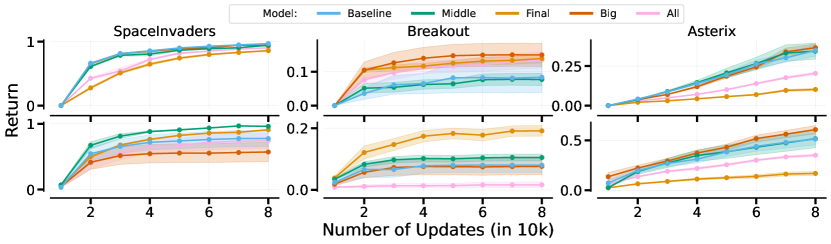
Figure 27: CRL: All TopK variants perform worse than the baseline except for Middle.

Game	Baseline	All	Big	Final	Middle
SI	$0.97\pm 0.01$	$0.86\pm 0.01$	$0.90\pm 0.01$	$0.94\pm 0.01$	$0.94\pm 0.01$
BO	$0.08\pm 0.05$	$0.14\pm 0.01$	$0.13\pm 0.02$	$0.15\pm 0.03$	$0.08\pm 0.02$
Ast	$0.35\pm 0.04$	$0.10\pm 0.01$	$0.20\pm 0.01$	$0.37\pm 0.02$	$0.34\pm 0.05$
SI-2	$0.78\pm 0.12$	$0.91\pm 0.01$	$0.74\pm 0.12$	$0.57\pm 0.15$	$0.96\pm 0.01$
BO-2	$0.08\pm 0.02$	$0.19\pm 0.02$	$0.02\pm 0.01$	$0.08\pm 0.03$	$0.10\pm 0.01$
Ast-2	$0.51\pm 0.06$	$0.17\pm 0.02$	$0.35\pm 0.02$	$0.61\pm 0.04$	$0.52\pm 0.09$
Total	$\mathbf{0.46\pm 0.03}$	$0.39\pm 0.01$	$0.39\pm 0.02$	$\mathbf{0.45\pm 0.02}$	$\mathbf{0.49\pm 0.02}$

Table 19: CRL: All TopK variants perform worse than the baseline except for Middle.

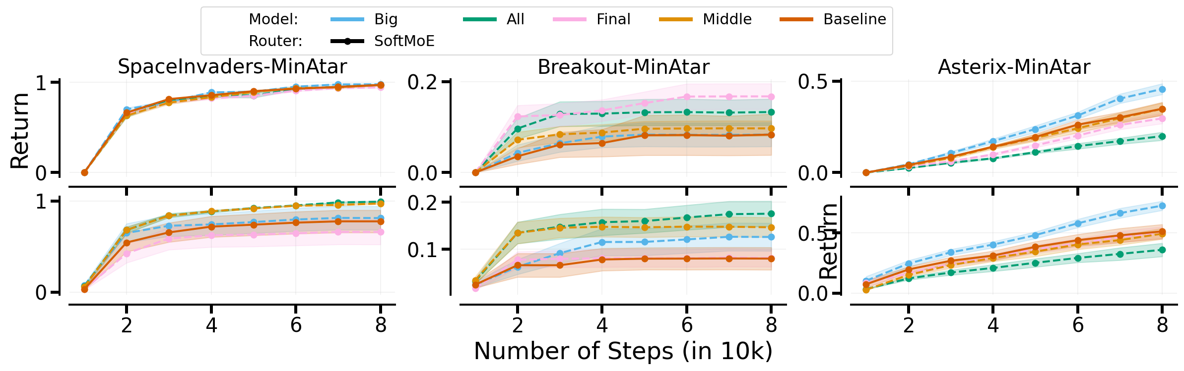
Figure 28: CRL: All SoftMoE Architectures: Big-SoftMoE is the only variant that performs better than the baseline.

Game	Baseline	All	Big	Final	Middle
SI	$0.97\pm 0.01$	$0.97\pm 0.01$	$0.98\pm 0.01$	$0.94\pm 0.01$	$0.97\pm 0.01$
BO	$0.08\pm 0.05$	$0.13\pm 0.03$	$0.08\pm 0.03$	$0.17\pm 0.03$	$0.10\pm 0.02$
Ast	$0.35\pm 0.04$	$0.20\pm 0.02$	$0.46\pm 0.03$	$0.30\pm 0.03$	$0.35\pm 0.03$
SI-2	$0.78\pm 0.12$	$0.99\pm 0.01$	$0.81\pm 0.13$	$0.66\pm 0.14$	$0.97\pm 0.01$
BO-2	$0.08\pm 0.02$	$0.18\pm 0.03$	$0.13\pm 0.03$	$0.08\pm 0.02$	$0.15\pm 0.02$
Ast-2	$0.51\pm 0.06$	$0.36\pm 0.06$	$0.73\pm 0.04$	$0.50\pm 0.05$	$0.49\pm 0.05$
Total	$\mathbf{0.46\pm 0.03}$	$0.47\pm 0.01$	$\mathbf{0.53\pm 0.02}$	$0.44\pm 0.03$	$\mathbf{0.50\pm 0.01}$

Table 20: CRL: All SoftMoE Architectures: Big-SoftMoE is the only variant that performs better than the baseline.

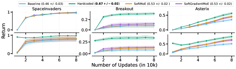
Figure 29: CRL: Adding gradient information to the input does not improve performance significantly.

Appendix G Single Env

height 75pt depth 0 pt width 0.8 pt

Game	Big-SoftMoE	Baseline	Big-Hardcoded	Big-TopK
SI	$0.98\pm 0.01$	$0.95\pm 0.01$	$0.94\pm 0.01$	$0.90\pm 0.01$
BO	$0.54\pm 0.09$	$0.66\pm 0.08$	$0.52\pm 0.07$	$0.54\pm 0.07$
Ast	$0.67\pm 0.03$	$0.58\pm 0.03$	$0.57\pm 0.03$	$0.32\pm 0.01$
Total	$\mathbf{0.73\pm 0.06}$	$\mathbf{0.73\pm 0.05}$	$\mathbf{0.67\pm 0.05}$	$0.59\pm 0.04$

Table 21: Single environment: Normalised Performance of algorithms across games with average total performance. We normalise performance according to the single environment results reported in Jesson et al. (2023). We do not achieve the same performance as we use smaller networks due to computational limits.

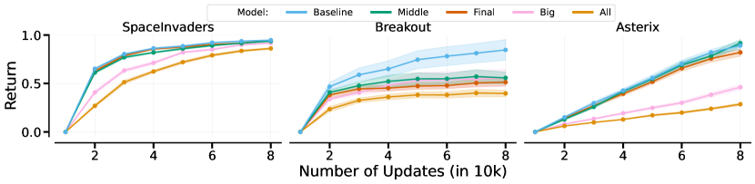
Figure 31: Single environment: All TopK Architectures, all variants perform worse than the baseline.

Game	All	Final	Middle	Baseline	Big
SI	$0.86\pm 0.01$	$0.94\pm 0.01$	$0.94\pm 0.00$	$0.95\pm 0.01$	$0.92\pm 0.01$
BO	$0.31\pm 0.03$	$0.40\pm 0.03$	$0.43\pm 0.05$	$0.66\pm 0.08$	$0.43\pm 0.07$
Ast	$0.19\pm 0.01$	$0.54\pm 0.02$	$0.60\pm 0.02$	$0.58\pm 0.03$	$0.30\pm 0.02$
Total	$0.45\pm 0.02$	$0.63\pm 0.02$	$\mathbf{0.66\pm 0.03}$	$\mathbf{0.73\pm 0.05}$	$0.55\pm 0.04$

Table 22: Single environment: All TopK Architectures, all variants perform worse than the baseline.

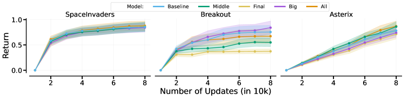
Figure 32: Single environment: All SoftMoE Architectures: Big, Final, and Middle all perform as well as the baseline.

Game	Big	All	Final	Baseline	Middle
SI	$0.98\pm 0.01$	$0.96\pm 0.00$	$0.94\pm 0.01$	$0.95\pm 0.01$	$0.95\pm 0.01$
BO	$0.54\pm 0.09$	$0.31\pm 0.02$	$0.67\pm 0.08$	$0.66\pm 0.08$	$0.44\pm 0.05$
Ast	$0.67\pm 0.03$	$0.55\pm 0.04$	$0.56\pm 0.03$	$0.58\pm 0.03$	$0.65\pm 0.02$
Total	$\mathbf{0.73\pm 0.06}$	$0.61\pm 0.03$	$\mathbf{0.72\pm 0.05}$	$\mathbf{0.73\pm 0.05}$	$\mathbf{0.68\pm 0.03}$

Table 23: Single environment: All SoftMoE Architectures: Big, Final, and Middle all perform as well as the baseline.

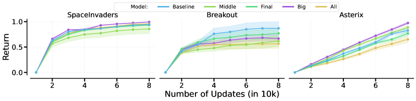
Figure 33: Single environment: All SoftGradientMoE Architectures., adding gradient information does not change the conclusions of the softmoe architectures above.

Game	Baseline	Middle	Big	Final	All
SI	$0.95\pm 0.01$	$0.86\pm 0.09$	$0.99\pm 0.00$	$0.93\pm 0.01$	$0.96\pm 0.01$
BO	$0.60\pm 0.09$	$0.42\pm 0.07$	$0.46\pm 0.04$	$0.53\pm 0.07$	$0.39\pm 0.06$
Ast	$0.59\pm 0.03$	$0.64\pm 0.03$	$0.70\pm 0.02$	$0.55\pm 0.03$	$0.47\pm 0.04$
Total	$\mathbf{0.71\pm 0.05}$	$\mathbf{0.64\pm 0.07}$	$\mathbf{0.72\pm 0.03}$	$\mathbf{0.67\pm 0.05}$	$0.60\pm 0.04$

Table 24: Single environment: All SoftGradientMoE Architectures, adding gradient information does not change the conclusions of the softmoe architectures above.

Game	w/ Gradient Info	w/o Gradient Info
SI	$0.95\pm 0.01$	$0.95\pm 0.01$
BO	$0.66\pm 0.08$	$0.60\pm 0.09$
Ast	$0.58\pm 0.03$	$0.59\pm 0.03$
Total	$\mathbf{0.73\pm 0.05}$	$\mathbf{0.71\pm 0.05}$

Table 25: Baseline vs. Baseline with Gradient Information: Adding gradient information to the input of the baseline does not affect its performance.

Appendix H Hyperparameters

Hyperparameter	Value
Number of Environments	128
Learning Rate	9e-4
Steps	64
Total Timesteps	1e7
Updates	total_timesteps // num_steps // num_envs
Update Epochs	10
Minibatches	8
Minibatch Size	num_envs * num_steps // num_minibatches
GAE-$\gamma$	0.99
GAE-$\lambda$	0.7
Clip $\epsilon$	0.2
Entropy Coefficient	0.01
Value Function Coeffficient	0.5
Max Gradient Norm	1.9
Activation	relu
Environment	{SpaceInvaders-MinAtar, Breakout-Minatar, Asterix-MinAtar}
Anneal learning rate	True
# Experts	3
Layer Size	64
Expert Hidden Size	64
Model	{BigMoE, FinalLayer, AllLayers, MiddleLayer}
MoE	{SoftMoE, MoE, SoftGradientMoE}
Expert	{BigExpert, Expert}
Router	{TopKRouter, HardcodedRouter}
Number of Selected Experts	1
Task ID	{True, False}
Actor MoE	{True, False}
Critic MoE	{True, False}
Gradient Buckets	5
Router Entropy	{True, False}

Table 26: Potential Hyperparameters configurations. We did not run a grid search over all potential combinations but report meaningful selections.

References

- Abbas & Andreopoulos (2020) Alhabib Abbas and Yiannis Andreopoulos. Biased mixtures of experts: Enabling computer vision inference under data transfer limitations. IEEE Transactions on Image Processing, 29:7656–7667, 2020.
- Abbas et al. (2023) Zaheer Abbas, Rosie Zhao, Joseph Modayil, Adam White, and Marlos C Machado. Loss of plasticity in continual deep reinforcement learning. arXiv preprint arXiv:2303.07507, 2023.
- Agarwal et al. (2020) Rishabh Agarwal, Dale Schuurmans, and Mohammad Norouzi. An optimistic perspective on offline reinforcement learning. In Hal Daumé III and Aarti Singh (eds.), Proceedings of the 37th International Conference on Machine Learning, volume 119 of Proceedings of Machine Learning Research, pp. 104–114. PMLR, 13–18 Jul 2020. URL https://proceedings.mlr.press/v119/agarwal20c.html.
- Agarwal et al. (2021) Rishabh Agarwal, Max Schwarzer, Pablo Samuel Castro, Aaron C Courville, and Marc Bellemare. Deep reinforcement learning at the edge of the statistical precipice. Advances in neural information processing systems, 34:29304–29320, 2021.
- Akrour et al. (2021) Riad Akrour, Davide Tateo, and Jan Peters. Continuous action reinforcement learning from a mixture of interpretable experts. IEEE Transactions on Pattern Analysis and Machine Intelligence, 44(10):6795–6806, 2021.
- An et al. (2021) Gaon An, Seungyong Moon, Jang-Hyun Kim, and Hyun Oh Song. Uncertainty-based offline reinforcement learning with diversified q-ensemble. Advances in neural information processing systems, 34:7436–7447, 2021.
- Anschel et al. (2016) Oron Anschel, Nir Baram, and Nahum Shimkin. Deep reinforcement learning with averaged target dqn. CoRR abs/1611.01929, 2016.
- Arnob et al. (2021) Samin Yeasar Arnob, Riyasat Ohib, Sergey Plis, and Doina Precup. Single-shot pruning for offline reinforcement learning. arXiv preprint arXiv:2112.15579, 2021.
- Bellemare et al. (2020) Marc G. Bellemare, Salvatore Candido, Pablo Samuel Castro, Jun Gong, Marlos C. Machado, Subhodeep Moitra, Sameera S. Ponda, and Ziyun Wang. Autonomous navigation of stratospheric balloons using reinforcement learning. Nature, 588:77 – 82, 2020.
- Bellman (1957) Richard Bellman. A markovian decision process. Journal of mathematics and mechanics, pp. 679–684, 1957.
- Berner et al. (2019) Christopher Berner, Greg Brockman, Brooke Chan, Vicki Cheung, Przemyslaw Debiak, Christy Dennison, David Farhi, Quirin Fischer, Shariq Hashme, Chris Hesse, et al. Dota 2 with large scale deep reinforcement learning. arXiv preprint arXiv:1912.06680, 2019.
- Bradbury et al. (2018) James Bradbury, Roy Frostig, Peter Hawkins, Matthew James Johnson, Chris Leary, Dougal Maclaurin, George Necula, Adam Paszke, Jake VanderPlas, Skye Wanderman-Milne, et al. Jax: composable transformations of python+ numpy programs. 2018.
- Ceron et al. (2024a) Johan Samir Obando Ceron, Aaron Courville, and Pablo Samuel Castro. In value-based deep reinforcement learning, a pruned network is a good network. In Forty-first International Conference on Machine Learning. PMLR, 2024a. URL https://openreview.net/forum?id=seo9V9QRZp.
- Ceron et al. (2024b) Johan Samir Obando Ceron, Ghada Sokar, Timon Willi, Clare Lyle, Jesse Farebrother, Jakob Nicolaus Foerster, Gintare Karolina Dziugaite, Doina Precup, and Pablo Samuel Castro. Mixtures of experts unlock parameter scaling for deep RL. In Forty-first International Conference on Machine Learning, 2024b. URL https://openreview.net/forum?id=X9VMhfFxwn.
- Chen et al. (2021) Xinyue Chen, Che Wang, Zijian Zhou, and Keith Ross. Randomized ensembled double q-learning: Learning fast without a model. arXiv preprint arXiv:2101.05982, 2021.
- Chen et al. (2023) Zitian Chen, Yikang Shen, Mingyu Ding, Zhenfang Chen, Hengshuang Zhao, Erik G Learned-Miller, and Chuang Gan. Mod-squad: Designing mixtures of experts as modular multi-task learners. In Proceedings of the IEEE/CVF Conference on Computer Vision and Pattern Recognition, pp. 11828–11837, 2023.
- Chua et al. (2018) Kurtland Chua, Roberto Calandra, Rowan McAllister, and Sergey Levine. Deep reinforcement learning in a handful of trials using probabilistic dynamics models. Advances in neural information processing systems, 31, 2018.
- Dohare et al. (2021) Shibhansh Dohare, Richard S Sutton, and A Rupam Mahmood. Continual backprop: Stochastic gradient descent with persistent randomness. arXiv preprint arXiv:2108.06325, 2021.
- D’Oro et al. (2022) Pierluca D’Oro, Max Schwarzer, Evgenii Nikishin, Pierre-Luc Bacon, Marc G Bellemare, and Aaron Courville. Sample-efficient reinforcement learning by breaking the replay ratio barrier. In Deep Reinforcement Learning Workshop NeurIPS 2022, 2022.
- Ellis et al. (2024) Benjamin Ellis, Jonathan Cook, Skander Moalla, Mikayel Samvelyan, Mingfei Sun, Anuj Mahajan, Jakob Foerster, and Shimon Whiteson. Smacv2: An improved benchmark for cooperative multi-agent reinforcement learning. Advances in Neural Information Processing Systems, 36, 2024.
- Evci et al. (2020) Utku Evci, Trevor Gale, Jacob Menick, Pablo Samuel Castro, and Erich Elsen. Rigging the lottery: Making all tickets winners. In Hal Daumé III and Aarti Singh (eds.), Proceedings of the 37th International Conference on Machine Learning, volume 119 of Proceedings of Machine Learning Research, pp. 2943–2952. PMLR, 13–18 Jul 2020. URL https://proceedings.mlr.press/v119/evci20a.html.
- Fan et al. (2023) Jiajun Fan, Yuzheng Zhuang, Yuecheng Liu, Jianye Hao, Bin Wang, Jiangcheng Zhu, Hao Wang, and Shu-Tao Xia. Learnable behavior control: Breaking atari human world records via sample-efficient behavior selection. arXiv preprint arXiv:2305.05239, 2023.
- Farebrother et al. (2024) Jesse Farebrother, Jordi Orbay, Quan Vuong, Adrien Ali Taïga, Yevgen Chebotar, Ted Xiao, Alex Irpan, Sergey Levine, Pablo Samuel Castro, Aleksandra Faust, Aviral Kumar, and Rishabh Agarwal. Stop regressing: Training value functions via classification for scalable deep rl. In Forty-first International Conference on Machine Learning. PMLR, 2024.
- Fawzi et al. (2022) Alhussein Fawzi, Matej Balog, Aja Huang, Thomas Hubert, Bernardino Romera-Paredes, Mohammadamin Barekatain, Alexander Novikov, Francisco J R Ruiz, Julian Schrittwieser, Grzegorz Swirszcz, et al. Discovering faster matrix multiplication algorithms with reinforcement learning. Nature, 610(7930):47–53, 2022.
- Fedus et al. (2022) William Fedus, Barret Zoph, and Noam Shazeer. Switch transformers: Scaling to trillion parameter models with simple and efficient sparsity. The Journal of Machine Learning Research, 23(1):5232–5270, 2022.
- Gale et al. (2019) Trevor Gale, Erich Elsen, and Sara Hooker. The state of sparsity in deep neural networks. CoRR, abs/1902.09574, 2019. URL http://arxiv.org/abs/1902.09574.
- Gale et al. (2023) Trevor Gale, Deepak Narayanan, Cliff Young, and Matei Zaharia. MegaBlocks: Efficient Sparse Training with Mixture-of-Experts. Proceedings of Machine Learning and Systems, 5, 2023.
- Graesser et al. (2022) Laura Graesser, Utku Evci, Erich Elsen, and Pablo Samuel Castro. The state of sparse training in deep reinforcement learning. In Kamalika Chaudhuri, Stefanie Jegelka, Le Song, Csaba Szepesvari, Gang Niu, and Sivan Sabato (eds.), Proceedings of the 39th International Conference on Machine Learning, volume 162 of Proceedings of Machine Learning Research, pp. 7766–7792. PMLR, 17–23 Jul 2022. URL https://proceedings.mlr.press/v162/graesser22a.html.
- Gupta et al. (2022) Shashank Gupta, Subhabrata Mukherjee, Krishan Subudhi, Eduardo Gonzalez, Damien Jose, Ahmed H Awadallah, and Jianfeng Gao. Sparsely activated mixture-of-experts are robust multi-task learners. arXiv preprint arXiv:2204.07689, 2022.
- Harris et al. (2020) Charles R Harris, K Jarrod Millman, Stéfan J Van Der Walt, Ralf Gommers, Pauli Virtanen, David Cournapeau, Eric Wieser, Julian Taylor, Sebastian Berg, Nathaniel J Smith, et al. Array programming with numpy. Nature, 585(7825):357–362, 2020.
- Hazimeh et al. (2021) Hussein Hazimeh, Zhe Zhao, Aakanksha Chowdhery, Maheswaran Sathiamoorthy, Yihua Chen, Rahul Mazumder, Lichan Hong, and Ed Chi. Dselect-k: Differentiable selection in the mixture of experts with applications to multi-task learning. Advances in Neural Information Processing Systems, 34:29335–29347, 2021.
- Hendawy et al. (2024) Ahmed Hendawy, Jan Peters, and Carlo D’Eramo. Multi-task reinforcement learning with mixture of orthogonal experts. In The Twelfth International Conference on Learning Representations, 2024. URL https://openreview.net/forum?id=aZH1dM3GOX.
- Houlsby et al. (2019) Neil Houlsby, Andrei Giurgiu, Stanislaw Jastrzebski, Bruna Morrone, Quentin De Laroussilhe, Andrea Gesmundo, Mona Attariyan, and Sylvain Gelly. Parameter-efficient transfer learning for NLP. In Kamalika Chaudhuri and Ruslan Salakhutdinov (eds.), Proceedings of the 36th International Conference on Machine Learning, volume 97 of Proceedings of Machine Learning Research, pp. 2790–2799. PMLR, 09–15 Jun 2019. URL https://proceedings.mlr.press/v97/houlsby19a.html.
- Hunter (2007) John D Hunter. Matplotlib: A 2d graphics environment. Computing in science & engineering, 9(03):90–95, 2007.
- Igl et al. (2020) Maximilian Igl, Gregory Farquhar, Jelena Luketina, Wendelin Boehmer, and Shimon Whiteson. Transient non-stationarity and generalisation in deep reinforcement learning. In International Conference on Learning Representations, 2020.
- Jacobs et al. (1991) Robert A Jacobs, Michael I Jordan, Steven J Nowlan, and Geoffrey E Hinton. Adaptive mixtures of local experts. Neural computation, 3(1):79–87, 1991.
- Jesson et al. (2023) Andrew Jesson, Chris Lu, Gunshi Gupta, Angelos Filos, Jakob Nicolaus Foerster, and Yarin Gal. Relu to the rescue: Improve your on-policy actor-critic with positive advantages. arXiv preprint arXiv:2306.01460, 2023.
- Jin et al. (2022) Tian Jin, Michael Carbin, Dan Roy, Jonathan Frankle, and Gintare Karolina Dziugaite. Pruning’s effect on generalization through the lens of training and regularization. Advances in Neural Information Processing Systems, 35:37947–37961, 2022.
- Khan et al. (2023) Akbir Khan, Timon Willi, Newton Kwan, Andrea Tacchetti, Chris Lu, Edward Grefenstette, Tim Rocktäschel, and Jakob Foerster. Scaling opponent shaping to high dimensional games. arXiv preprint arXiv:2312.12568, 2023.
- Khetarpal et al. (2022) Khimya Khetarpal, Matthew Riemer, Irina Rish, and Doina Precup. Towards continual reinforcement learning: A review and perspectives. Journal of Artificial Intelligence Research, 75:1401–1476, 2022.
- Kluyver et al. (2016) Thomas Kluyver, Benjain Ragan-Kelley, Fernando Pérez, Brian Granger, Matthias Bussonnier, Jonathan Frederic, Kyle Kelley, Jessica Hamrick, Jason Grout, Sylvain Corlay, Paul Ivanov, Damián Avila, Safia Abdalla, Carol Willing, and Jupyter Development Team. Jupyter Notebooks—a publishing format for reproducible computational workflows. In IOS Press, pp. 87–90. 2016. doi: 10.3233/978-1-61499-649-1-87.
- Kumar et al. (2021) Aviral Kumar, Rishabh Agarwal, Dibya Ghosh, and Sergey Levine. Implicit under-parameterization inhibits data-efficient deep reinforcement learning. In International Conference on Learning Representations, 2021. URL https://openreview.net/forum?id=O9bnihsFfXU.
- Kurutach et al. (2018) Thanard Kurutach, Ignasi Clavera, Yan Duan, Aviv Tamar, and Pieter Abbeel. Model-ensemble trust-region policy optimization. arXiv preprint arXiv:1802.10592, 2018.
- Lan et al. (2020) Qingfeng Lan, Yangchen Pan, Alona Fyshe, and Martha White. Maxmin q-learning: Controlling the estimation bias of q-learning. arXiv preprint arXiv:2002.06487, 2020.
- Lange (2022) Robert Tjarko Lange. gymnax: A JAX-based reinforcement learning environment library, 2022. URL http://github.com/RobertTLange/gymnax.
- Lepikhin et al. (2020) Dmitry Lepikhin, HyoukJoong Lee, Yuanzhong Xu, Dehao Chen, Orhan Firat, Yanping Huang, Maxim Krikun, Noam Shazeer, and Zhifeng Chen. Gshard: Scaling giant models with conditional computation and automatic sharding. In International Conference on Learning Representations, 2020.
- Lewis et al. (2021) Mike Lewis, Shruti Bhosale, Tim Dettmers, Naman Goyal, and Luke Zettlemoyer. Base layers: Simplifying training of large, sparse models. In International Conference on Machine Learning, 2021. URL https://api.semanticscholar.org/CorpusID:232428341.
- Liang et al. (2022) Litian Liang, Yaosheng Xu, Stephen McAleer, Dailin Hu, Alexander Ihler, Pieter Abbeel, and Roy Fox. Reducing variance in temporal-difference value estimation via ensemble of deep networks. In International Conference on Machine Learning, pp. 13285–13301. PMLR, 2022.
- Lu et al. (2022a) Chris Lu, Jakub Kuba, Alistair Letcher, Luke Metz, Christian Schroeder de Witt, and Jakob Foerster. Discovered policy optimisation. Advances in Neural Information Processing Systems, 35:16455–16468, 2022a.
- Lu et al. (2023) Chris Lu, Timon Willi, Alistair Letcher, and Jakob Nicolaus Foerster. Adversarial cheap talk. In International Conference on Machine Learning, pp. 22917–22941. PMLR, 2023.
- Lu et al. (2022b) Christopher Lu, Timon Willi, Christian A Schroeder De Witt, and Jakob Foerster. Model-free opponent shaping. In International Conference on Machine Learning, pp. 14398–14411. PMLR, 2022b.
- Lyle et al. (2022) Clare Lyle, Mark Rowland, and Will Dabney. Understanding and preventing capacity loss in reinforcement learning. In International Conference on Learning Representations, 2022. URL https://openreview.net/forum?id=ZkC8wKoLbQ7.
- Lyle et al. (2023) Clare Lyle, Zeyu Zheng, Evgenii Nikishin, Bernardo Ávila Pires, Razvan Pascanu, and Will Dabney. Understanding plasticity in neural networks. In Andreas Krause, Emma Brunskill, Kyunghyun Cho, Barbara Engelhardt, Sivan Sabato, and Jonathan Scarlett (eds.), International Conference on Machine Learning, ICML 2023, 23-29 July 2023, Honolulu, Hawaii, USA, volume 202 of Proceedings of Machine Learning Research, pp. 23190–23211. PMLR, 2023. URL https://proceedings.mlr.press/v202/lyle23b.html.
- McKinney (2013) Wes McKinney. Python for Data Analysis: Data Wrangling with Pandas, NumPy, and IPython. O’Reilly Media, 1 edition, February 2013. ISBN 9789351100065. URL http://www.amazon.com/exec/obidos/redirect?tag=citeulike07-20&path=ASIN/1449319793.
- Mnih et al. (2015) Volodymyr Mnih, Koray Kavukcuoglu, David Silver, Andrei A. Rusu, Joel Veness, Marc G. Bellemare, Alex Graves, Martin Riedmiller, Andreas K. Fidjeland, Georg Ostrovski, Stig Petersen, Charles Beattie, Amir Sadik, Ioannis Antonoglou, Helen King, Dharshan Kumaran, Daan Wierstra, Shane Legg, and Demis Hassabis. Human-level control through deep reinforcement learning. Nature, 518(7540):529–533, February 2015.
- Nikishin et al. (2022a) Evgenii Nikishin, Max Schwarzer, Pierluca D’Oro, Pierre-Luc Bacon, and Aaron Courville. The primacy bias in deep reinforcement learning. In Kamalika Chaudhuri, Stefanie Jegelka, Le Song, Csaba Szepesvari, Gang Niu, and Sivan Sabato (eds.), Proceedings of the 39th International Conference on Machine Learning, volume 162 of Proceedings of Machine Learning Research, pp. 16828–16847. PMLR, 17–23 Jul 2022a. URL https://proceedings.mlr.press/v162/nikishin22a.html.
- Nikishin et al. (2022b) Evgenii Nikishin, Max Schwarzer, Pierluca D’Oro, Pierre-Luc Bacon, and Aaron Courville. The primacy bias in deep reinforcement learning. In International conference on machine learning, pp. 16828–16847. PMLR, 2022b.
- Obando Ceron et al. (2023) Johan Obando Ceron, Marc Bellemare, and Pablo Samuel Castro. Small batch deep reinforcement learning. In A. Oh, T. Naumann, A. Globerson, K. Saenko, M. Hardt, and S. Levine (eds.), Advances in Neural Information Processing Systems, volume 36, pp. 26003–26024. Curran Associates, Inc., 2023. URL https://proceedings.neurips.cc/paper_files/paper/2023/file/528388f1ad3a481249a97cbb698d2fe6-Paper-Conference.pdf.
- Obando-Ceron & Castro (2021) Johan Samir Obando-Ceron and Pablo Samuel Castro. Revisiting rainbow: Promoting more insightful and inclusive deep reinforcement learning research. In Marina Meila and Tong Zhang (eds.), Proceedings of the 38th International Conference on Machine Learning, volume 139 of Proceedings of Machine Learning Research, pp. 1373–1383. PMLR, 18–24 Jul 2021. URL https://proceedings.mlr.press/v139/ceron21a.html.
- Oliphant (2007) Travis E. Oliphant. Python for scientific computing. Computing in Science & Engineering, 9(3):10–20, 2007. doi: 10.1109/MCSE.2007.58.
- Ostrovski et al. (2021) Georg Ostrovski, Pablo Samuel Castro, and Will Dabney. The difficulty of passive learning in deep reinforcement learning. In A. Beygelzimer, Y. Dauphin, P. Liang, and J. Wortman Vaughan (eds.), Advances in Neural Information Processing Systems, 2021. URL https://openreview.net/forum?id=nPHA8fGicZk.
- Pavlitskaya et al. (2020) Svetlana Pavlitskaya, Christian Hubschneider, Michael Weber, Ruby Moritz, Fabian Huger, Peter Schlicht, and Marius Zollner. Using mixture of expert models to gain insights into semantic segmentation. In Proceedings of the IEEE/CVF Conference on Computer Vision and Pattern Recognition Workshops, pp. 342–343, 2020.
- Peer et al. (2021) Oren Peer, Chen Tessler, Nadav Merlis, and Ron Meir. Ensemble bootstrapping for q-learning. In International Conference on Machine Learning, pp. 8454–8463. PMLR, 2021.
- Puigcerver et al. (2023) Joan Puigcerver, Carlos Riquelme, Basil Mustafa, and Neil Houlsby. From sparse to soft mixtures of experts, 2023.
- Puterman (1990) Martin L Puterman. Markov decision processes. Handbooks in operations research and management science, 2:331–434, 1990.
- Ren et al. (2021) Jie Ren, Yewen Li, Zihan Ding, Wei Pan, and Hao Dong. Probabilistic mixture-of-experts for efficient deep reinforcement learning. arXiv preprint arXiv:2104.09122, 2021.
- Rutherford et al. (2023) Alexander Rutherford, Benjamin Ellis, Matteo Gallici, Jonathan Cook, Andrei Lupu, Gardar Ingvarsson, Timon Willi, Akbir Khan, Christian Schroeder de Witt, Alexandra Souly, et al. Jaxmarl: Multi-agent rl environments in jax. arXiv preprint arXiv:2311.10090, 2023.
- Schulman et al. (2017) John Schulman, Filip Wolski, Prafulla Dhariwal, Alec Radford, and Oleg Klimov. Proximal policy optimization algorithms. arXiv preprint arXiv:1707.06347, 2017.
- Schwarzer et al. (2023) Max Schwarzer, Johan Samir Obando-Ceron, Aaron Courville, Marc G Bellemare, Rishabh Agarwal, and Pablo Samuel Castro. Bigger, better, faster: Human-level Atari with human-level efficiency. In Andreas Krause, Emma Brunskill, Kyunghyun Cho, Barbara Engelhardt, Sivan Sabato, and Jonathan Scarlett (eds.), Proceedings of the 40th International Conference on Machine Learning, volume 202 of Proceedings of Machine Learning Research, pp. 30365–30380. PMLR, 23–29 Jul 2023. URL https://proceedings.mlr.press/v202/schwarzer23a.html.
- Shazeer et al. (2017) Noam Shazeer, *Azalia Mirhoseini, *Krzysztof Maziarz, Andy Davis, Quoc Le, Geoffrey Hinton, and Jeff Dean. Outrageously large neural networks: The sparsely-gated mixture-of-experts layer. In International Conference on Learning Representations, 2017. URL https://openreview.net/forum?id=B1ckMDqlg.
- Shyam et al. (2019) Pranav Shyam, Wojciech Jaśkowski, and Faustino Gomez. Model-based active exploration. In International conference on machine learning, pp. 5779–5788. PMLR, 2019.
- Sokar et al. (2022) Ghada Sokar, Elena Mocanu, Decebal Constantin Mocanu, Mykola Pechenizkiy, and Peter Stone. Dynamic sparse training for deep reinforcement learning. In International Joint Conference on Artificial Intelligence, 2022.
- Sokar et al. (2023) Ghada Sokar, Rishabh Agarwal, Pablo Samuel Castro, and Utku Evci. The dormant neuron phenomenon in deep reinforcement learning. In Andreas Krause, Emma Brunskill, Kyunghyun Cho, Barbara Engelhardt, Sivan Sabato, and Jonathan Scarlett (eds.), Proceedings of the 40th International Conference on Machine Learning, volume 202 of Proceedings of Machine Learning Research, pp. 32145–32168. PMLR, 23–29 Jul 2023. URL https://proceedings.mlr.press/v202/sokar23a.html.
- Sutton & Barto (2018) Richard S Sutton and Andrew G Barto. Reinforcement learning: An introduction. MIT press, 2018.
- Tan et al. (2022) Yiqin Tan, Pihe Hu, Ling Pan, Jiatai Huang, and Longbo Huang. Rlx2: Training a sparse deep reinforcement learning model from scratch. In The Eleventh International Conference on Learning Representations, 2022.
- Van Rossum & Drake Jr (1995) Guido Van Rossum and Fred L Drake Jr. Python reference manual. Centrum voor Wiskunde en Informatica Amsterdam, 1995.
- Vaswani et al. (2017) Ashish Vaswani, Noam Shazeer, Niki Parmar, Jakob Uszkoreit, Llion Jones, Aidan N Gomez, Ł ukasz Kaiser, and Illia Polosukhin. Attention is all you need. In I. Guyon, U. Von Luxburg, S. Bengio, H. Wallach, R. Fergus, S. Vishwanathan, and R. Garnett (eds.), Advances in Neural Information Processing Systems, volume 30. Curran Associates, Inc., 2017.
- Vinyals et al. (2019) Oriol Vinyals, Igor Babuschkin, Wojciech M Czarnecki, Michaël Mathieu, Andrew Dudzik, Junyoung Chung, David H Choi, Richard Powell, Timo Ewalds, Petko Georgiev, et al. Grandmaster level in starcraft ii using multi-agent reinforcement learning. Nature, 575(7782):350–354, 2019.
- Wang et al. (2020) Xin Wang, Fisher Yu, Lisa Dunlap, Yi-An Ma, Ruth Wang, Azalia Mirhoseini, Trevor Darrell, and Joseph E Gonzalez. Deep mixture of experts via shallow embedding. In Uncertainty in artificial intelligence, pp. 552–562. PMLR, 2020.
- Willi et al. (2022) Timon Willi, Alistair Hp Letcher, Johannes Treutlein, and Jakob Foerster. Cola: consistent learning with opponent-learning awareness. In International Conference on Machine Learning, pp. 23804–23831. PMLR, 2022.
- Wu et al. (2021) Yanqiu Wu, Xinyue Chen, Che Wang, Yiming Zhang, and Keith W Ross. Aggressive q-learning with ensembles: Achieving both high sample efficiency and high asymptotic performance. arXiv preprint arXiv:2111.09159, 2021.
- Yang et al. (2019) Brandon Yang, Gabriel Bender, Quoc V Le, and Jiquan Ngiam. Condconv: Conditionally parameterized convolutions for efficient inference. Advances in neural information processing systems, 32, 2019.
- Ye & Xu (2023) Hanrong Ye and Dan Xu. Taskexpert: Dynamically assembling multi-task representations with memorial mixture-of-experts. In Proceedings of the IEEE/CVF International Conference on Computer Vision, pp. 21828–21837, 2023.
- Young & Tian (2019) Kenny Young and Tian Tian. Minatar: An atari-inspired testbed for thorough and reproducible reinforcement learning experiments. arXiv preprint arXiv:1903.03176, 2019.
- Zhou et al. (2022) Yanqi Zhou, Tao Lei, Hanxiao Liu, Nan Du, Yanping Huang, Vincent Zhao, Andrew M Dai, Quoc V Le, James Laudon, et al. Mixture-of-experts with expert choice routing. Advances in Neural Information Processing Systems, 35:7103–7114, 2022.
- Zoph et al. (2022) Barret Zoph, Irwan Bello, Sameer Kumar, Nan Du, Yanping Huang, Jeff Dean, Noam Shazeer, and William Fedus. St-moe: Designing stable and transferable sparse expert models, 2022.