Aligning Diffusion Models with Noise-Conditioned Perception

Abstract

Recent advancements in human preference optimization, initially developed for Language Models (LMs), have shown promise for text-to-image Diffusion Models, enhancing prompt alignment, visual appeal, and user preference. Unlike LMs, Diffusion Models typically optimize in pixel or VAE space, which does not align well with human perception, leading to slower and less efficient training during the preference alignment stage. We propose using a perceptual objective in the U-Net embedding space of the diffusion model to address these issues. Our approach involves fine-tuning Stable Diffusion 1.5 and XL using Direct Preference Optimization (DPO), Contrastive Preference Optimization (CPO), and supervised fine-tuning (SFT) within this embedding space. This method significantly outperforms standard latent-space implementations across various metrics, including quality and computational cost. For SDXL, our approach provides 60.8% general preference, 62.2% visual appeal, and 52.1% prompt following against original open-sourced SDXL-DPO on the PartiPrompts dataset, while significantly reducing compute. Our approach not only improves the efficiency and quality of human preference alignment for diffusion models but is also easily integrable with other optimization techniques. The training code and LoRA weights will be available here: https://huggingface.co/alexgambashidze/SDXL_NCP-DPO_v0.1

In generative NLP, recent research has shown the benefits of alignment, the process of fine-tuning a generative model to some specific objective, particularly human preference [44, 26]. One of the most popular and prominent methods is Direct Preference Optimization (DPO), which involves fine-tuning a model on a dataset of ranked pairs of samples [26]. DPO has achieved substantial progress in alignment of Large Language Models, due to being supervised and simple, compared to hyperparameter-heavy RL methods like RLHF [44]. Recently DPO has been adapted to Diffusion Models, significantly improving overall preference, prompt following, aesthetics, and structure of images [34].

Pretrained Language Models have inherently highly semantic embedding spaces, which naturally suits contrastive objectives like DPO. Diffusion Models, however, are trained to predict image-space noise, and image space does not possess any semantic or perceptual structure [42]. Latent Diffusion models bring diffusion process into latent space of a Variational Autoencoder (VAE) [27], but the rationale for that is to only abstract away imperceptible details and reduce computation, as those latent spaces still carry spatial details. On the other hand, it is a well-known fact that pretrained deep vision networks’ embedding spaces are highly perceptual, i.e. being able to grasp high-level properties of images [42]. This discrepancy motivates us to seek a perceptual objective for diffusion model alignment.

There have been attempts to equip diffusion model training objective with some form of perceptual loss [41]. These losses are implemented by denoising from noise level $t$ to the initial sample $x_{0}$, decoding it with VAE, and then feeding it into a corresponding vision network. However, this process is difficult in optimization and introduces several out-of-distribution approximations.

Importantly, recent advancements have revealed that diffusion model U-Net backbone, a deep pre-trained vision model itself, possess embedding space with perceptual properties [36, 43, 37]. The paper <<Diffusion Model with Perceptual Loss>> [18] proposes utilizing this embedding space for pretraining and achieve improved results. We propose leveraging a noise-conditioned perceptual loss similar to [18] for preference optimization. Specifically, we utilize the pretrained encoder of a denoising U-Net, which operates in a noise-conditioned embedding space. This approach allows us to bypass the pitfalls of pixel-space optimization and directly align with human perceptual features, while significantly accelerating the training process.

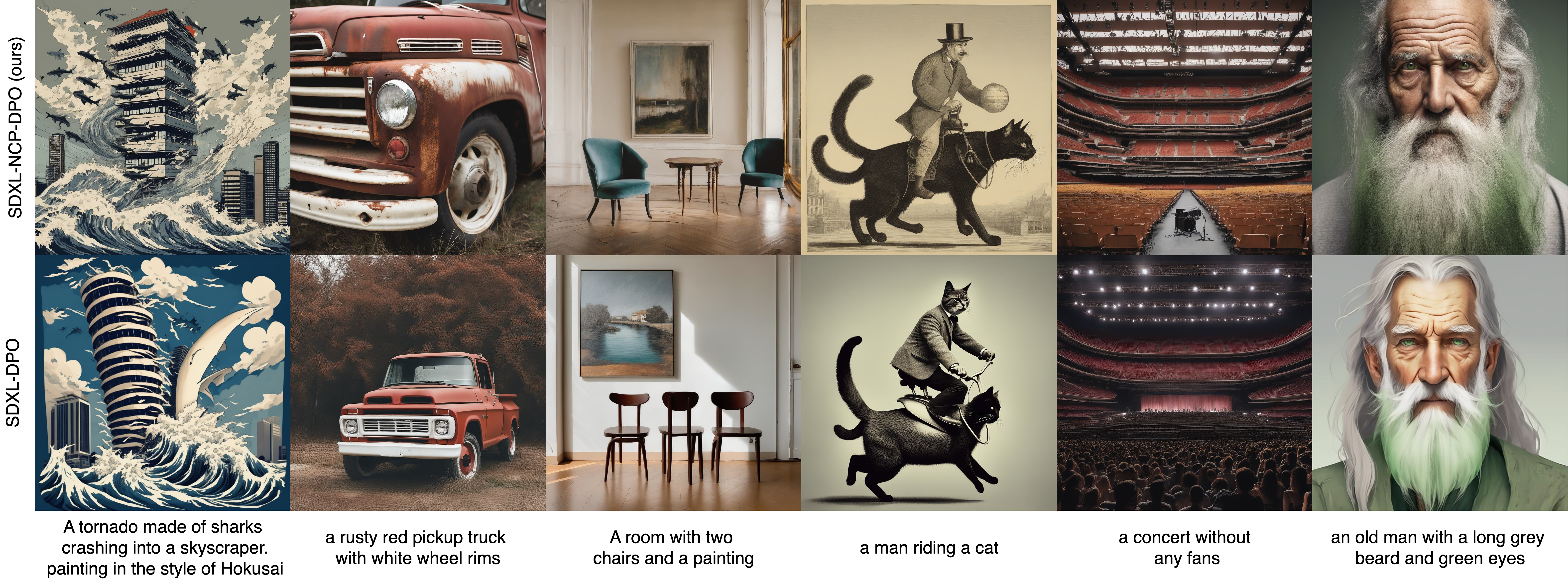
Figure 1: Noise-Conditioned Perceptual objective for aligning diffusion models improves Direct Preference Optimization in both Visual Appeal and Prompt Following.

Our contributions are as follows:

1. Noise-Conditioned Perceptual Preference Optimization (NCPPO): We introduce NCPPO, a method that utilizes the U-Net encoder’s embedding space for preference optimization. This approach aligns the optimization process with human perceptual features, rather than the less informative pixel space. It can be seamlessly combined with Direct Preference Optimization (DPO), Contrastive Preference Optimization (CPO), and Supervised Fine-Tuning (SFT), further enhancing their effectiveness.

2. Enhanced Training Efficiency: Our method significantly reduces the computational resources and training time required for preference optimization. For example, we achieve superior performance using only 2% of the aligning compute compared to existing methods.

3. Improved Model Performance: We demonstrate that our approach significantly outperforms standard latent-space Direct Preference Optimization in terms of human evaluation metrics. Our fine-tuning of Stable Diffusion 1.5 and XL models shows marked improvements in prompt alignment, visual appeal, and overall user preference.

By embedding the preference optimization process within a noise-conditioned perceptual space, we provide a more natural and efficient method for aligning diffusion models with human preferences. Our results indicate that this approach not only improves the quality of generated images but also significantly reduces the computational burden, making it a promising direction for future research and practical applications.

1 Related Works

Diffusion Model Fine-Tuning:

There are various approaches to fine-tuning diffusion models to better align with specific objectives, like conditions or preferences. One class of methods uses gradients of explicit reward functions. Classifier Guidance [5, 32] proposes an inference-time technique to guide generations towards desirable regions using gradients of a classifier, but this method requires a noise-conditioned classifier network [11], which makes it impractical. Unified Guidance [1, 22] instead uses intermediate denoised predictions as inputs for an off-the-shelf classifier, but these predictions are often out-of-distribution for most vision models due to nonlinearity in sampling trajectories.

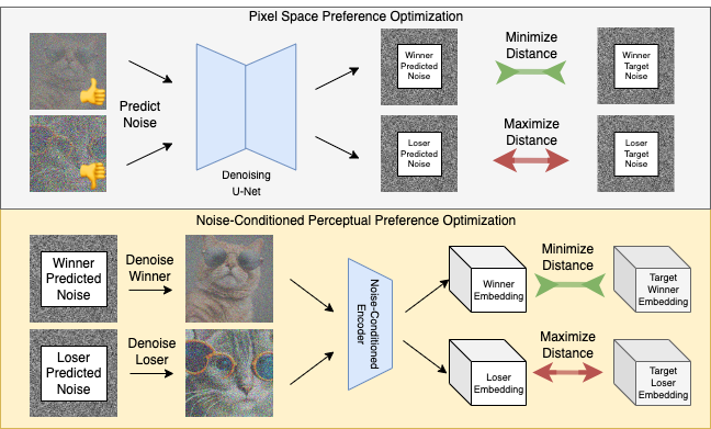
Figure 2: Overall NCPPO pipeline. We optimize preferences inside a Noise-Conditioned embedding space.

Training-time techniques like DRaFT [4], ReFL [39], and AlignProp [25] optimize for the maximum differentiable reward by backpropagating gradients through the entire sampling process, which requires substantial GPU memory.

Similar to RLHF in language models [44], a number of works employ Reinforcement Learning (RL) for reward optimization [2, 7]. These methods frame the generation process as a Markov Decision Process (MDP) with the noise predictor network as an agent, using variants of Policy Gradient [30] with KL-regularized rewards [3]. While not requiring differentiable rewards, these methods are often unstable and prone to reward hacking.

Direct Preference Optimization:

First proposed for language models, DPO sidesteps the unstable and complex RL methods by rewriting the RLHF objective in terms of implicit optimal reward [26]. Diffusion-DPO [34] extends this to diffusion models, using conditional score matching objectives for efficient training. A lot of effort has been put into improving DPO procedure (mainly in the context of LLMs), like elucidating sources for preference data [20, 33], using listwise instead of pairwise losses [19, 31], either training, getting rid of, or replacing reference model [38, 12, 8]. Despite these experiments in the field of NLP, almost nothing specific to text-to-image diffusion models have been proposed in this area.

Diffusion U-Net Properties:

Pretrained deep image networks, including U-Nets, possess rich, transferable latent spaces applicable to downstream tasks [42]. Recently, diffusion model backbones have been shown to be no exception. U-Net [28] or DiT [23] backbones trained with diffusion objective can be a good initialization for fine-tuning on downstream image-to-image tasks, such as semantic segmentation or depth estimation [43, 37], as well as used for classification with minimal training [36]. Noise-conditioned classifiers for Classifier Guidance were initialized with U-Net in the original work [5]. Finally, features from U-Net cross-attention have been extensively manipulated to achieve controlled generation and editing [9, 6, 16].

By leveraging these insights, our work proposes using the U-Net encoder’s embedding space for preference optimization in diffusion models, offering a more efficient and perceptually aligned training process.

2 Preliminaries

Diffusion models are latent-variable generative models that generate data by iteratively denoising a sample from Gaussian noise [10]. The core idea is to model the data distribution with a two-way Markov chain of gradually noised/denoised latent variables. The diffusion model formulation consists of a fixed forward process, which takes a sample from the data distribution and progressively corrupts it with Gaussian noise, and a parametric reverse process that learns to revert this corruption and effectively recover samples from the data distribution.

In the forward process, a data point $\mathbf{x}_{0}$ is transformed into a noisy version $\mathbf{x}_{t}$ over $T$ discrete timesteps. At each timestep $t$, noise is incrementally added according to a predefined variance schedule $\left\{\alpha_{t}\right\}_{0}^{T}$. In terms of samples, this process can be formulated as follows:

$$\mathbf{x}_{t}=\sqrt{\bar{\alpha}_{t}}\mathbf{x}_{0}+\sqrt{1-\bar{\alpha}_{t}}\epsilon,\quad\epsilon\sim\mathcal{N}(0,\mathbf{I})$$ (1)

The reverse process involves learning a model $\mathbf{\epsilon}_{\theta}$ that predicts the noise added at each step, directly recovering an estimate of $\mathbf{x}_{0}$. Transition to previous step sample $\mathbf{x}_{t-1}$ is defined by the DDPM reverse process as follows:

$$\mathbf{x}_{t-1}=\frac{1}{\sqrt{\alpha_{t}}}\Big{(}\mathbf{x}_{t}-\frac{1-\alpha_{t}}{\sqrt{1-\bar{\alpha}_{t}}}\mathbf{\epsilon}_{\theta}(\mathbf{x}_{t},t)\Big{)}+\sigma_{t}\mathbf{z},\quad\mathbf{z}\sim\mathcal{N}(0,\mathbf{I})$$ (2)

Diffusion denoising model $\mathbf{\epsilon}_{\theta}$ can be efficiently trained with SGD by minimizing the squared error between the true noise $\mathbf{\epsilon}$ and predicted noise $\mathbf{\epsilon}_{\theta}(\mathbf{x}_{t},t)$. Formally, this loss is defined as follows:

$$L_{\theta}=\left\lVert\mathbf{\epsilon}-\mathbf{\epsilon}_{\theta}(\mathbf{x}_{t},t)\right\rVert_{2}^{2},\quad\mathcal{L}(\theta)=\mathbb{E}_{\mathbf{x}\sim\mathcal{D}}\left[L_{\theta}\right]$$ (3)

After the denoising model is trained, sampling does not need to involve all $T$ steps and can utilize the SDE or score-based formulation of diffusion models [32, 14].

2.1 Preference Optimization

Next, we review Direct Preference Optimization (DPO) and Contrastive Preference Optimization (CPO) approaches for diffusion models, establishing the foundation for our proposed Noise-Conditioned Perceptual Preference Optimization (NCPPO).

The task of preference optimization is to fine-tune a generative model such that it produces samples more aligned to what humans find preferable. It is assumed that humans express preference according to a latent reward function $r^{*}$, and that there is a dataset $\mathcal{D}=\{(\mathbf{c},\mathbf{x}^{w},\mathbf{x}^{l})\}$, where $\mathbf{c}$ is a condition, and $\mathbf{x}^{w}$ and $\mathbf{x}^{l}$ are the preferred (winner) and dispreferred (loser) generated samples, respectively.

RLHF [3] first aims to obtain an explicit parameterized reward function $r_{\phi}$ by fitting Bradley-Terry model on the dataset $\mathcal{D}$ with maximum likelihood.

$$\mathcal{L}_{r}\left(r_{\phi},\mathcal{D}\right)=-\mathbb{E}_{\left(\mathbf{c},\mathbf{x}^{w},\mathbf{x}^{l}\right)\sim\mathcal{D}}\left[\log\sigma\left(r_{\phi}\left(\mathbf{c},\mathbf{x}^{w}\right)-r_{\phi}\left(\mathbf{c},\mathbf{x}^{l}\right)\right)\right]$$ (4)

With the fitted reward function, it is possible to use Reinforcement Learning to optimize the generative model $p_{\theta}(\mathbf{x}|\mathbf{c})$ as policy, and employ a form of Policy Gradient to optimize the model. Following [44], reward is also modified with regularization by adding KL-divergence term:

$$\max_{p_{\theta}}\mathbb{E}_{\mathbf{c}\sim\mathcal{D}_{c},\mathbf{x}\sim p_{\theta}\left(\mathbf{x}|\mathbf{c}\right)}{\left[r\left(\mathbf{c},\mathbf{x}\right)\right]}-\beta\mathbb{D}_{\mathrm{KL}}\left[p_{\theta}\left(\mathbf{x}|\mathbf{c}\right)\|p_{\mathrm{ref}}\left(\mathbf{x}|\mathbf{c}\right)\right]$$ (5)

DPO elegantly restates $L_{RLHF}$ without the need for RL Policy Gradient estimators. First, it considers the solution to the given optimization problem, optimal policy $p^{*}(\mathbf{x}|\mathbf{c})$ under reward function $r$, and rearranges it into an expression in terms of optimal policy:

$$p_{\theta}^{*}\left(\mathbf{x}|\mathbf{c}\right)=\frac{p_{\mathrm{ref}}\left(\mathbf{x}|\mathbf{c}\right)\exp\left(r\left(\mathbf{c},\mathbf{x}\right)/\beta\right)}{\sum_{\mathbf{x}}p_{\mathrm{ref}}\left(\mathbf{x}|\mathbf{c}\right)\exp\left(r\left(\mathbf{c},\mathbf{x}\right)/\beta\right)}$$ (6)

Plugging it into the Bradley-Terry model from equation 4, we arrive at the DPO objective:

$$\mathcal{L}_{\mathrm{DPO}}(\theta)=-\mathbb{E}_{\left(\mathbf{c},\mathbf{x}^{w},\mathbf{x}^{l}\right)\sim\mathcal{D}}\left[\log\sigma\left(\beta\log\frac{p_{\theta}(\mathbf{x}^{w}|\mathbf{c})}{p_{\mathrm{ref}}(\mathbf{x}^{w}|\mathbf{c})}-\beta\log\frac{p_{\theta}(\mathbf{x}^{l}|\mathbf{c})}{p_{\mathrm{ref}}(\mathbf{x}^{l}|\mathbf{c})}\right)\right]$$ (7)

Through several approximations and careful rearrangement of expectations using Jensen’s inequality, Wallace et al. [34] find a way to rewrite the DPO objective for diffusion models in the following form:

$$\mathcal{L}_{\mathrm{DiffusionDPO}}(\theta)=-\mathbb{E}_{\left(\mathbf{c},\mathbf{x}^{w},\mathbf{x}^{l}\right)\sim\mathcal{D}}\left[\log\sigma\left(-\beta T\left((L_{\theta}^{w}-L_{\mathrm{ref}}^{w})-(L_{\theta}^{l}-L_{\mathrm{ref}}^{l})\right)\right)\right]$$ (8)

where $L$ correspond to diffusion losses from 3, calculated over winners, losers, current and reference models, respectively.

Contrastive Policy Optimization (CPO) is derived from the DPO objective by substituting the reference policy $p_{ref}(x|\mathbf{c})$ with the optimal policy $p_{w}(x|\mathbf{c})$, defined such that $p_{w}(\mathbf{x}^{w}|\mathbf{c})$ = 1 and
0 $\leq$ $p_{w}(\mathbf{x}^{l}|\mathbf{c})$ $\leq$ 1. By incorporating this substitution into the original DPO objective, Xu et al. [38] derive the following formulation:

$$\mathcal{L}_{\mathrm{CPO}}(\theta)=-\mathbb{E}_{\left(\mathbf{c},\mathbf{x}^{w},\mathbf{x}^{l}\right)\sim\mathcal{D}}\left[\log\sigma\left(\beta\log p_{\theta}(\mathbf{x}^{w}|\mathbf{c})-\beta\log p_{\theta}(\mathbf{x}^{l}|\mathbf{c})+\beta\log p_{\mathrm{ref}}(\mathbf{x}^{l}|\mathbf{c})\right)\right]$$ (9)

After performing a series of intermediate calculations, the CPO objective simplifies to:

$$\mathcal{L}_{\mathrm{CPO}}(\theta)=-\mathbb{E}_{\left(\mathbf{c},\mathbf{x}^{w},\mathbf{x}^{l}\right)\sim\mathcal{D}}\left[\log\sigma\left(\beta\log p_{\theta}(\mathbf{x}^{w}|\mathbf{c})-\beta\log p_{\theta}(\mathbf{x}^{l}|\mathbf{c})\right)\right]-\lambda\mathbb{E}_{(\mathbf{c},\mathbf{x}^{w})\sim\mathcal{D}}\left[\beta\log p_{\theta}(\mathbf{x}^{w}|\mathbf{c})\right]$$ (10)

where the second term provides additional guidance for the policy. Applying this formulation to the diffusion problem results in the final objective:

$$\mathcal{L}_{\mathrm{DiffusionCPO}}(\theta)=-\mathbb{E}_{\left(\mathbf{c},\mathbf{x}^{w},\mathbf{x}^{l}\right)\sim\mathcal{D}}\left[\log\sigma\left(-\beta T\left(PL_{\theta}^{w}-PL_{\theta}^{l}\right)\right)\right]+\lambda\mathbb{E}_{(\mathbf{c},\mathbf{x}^{w})\sim\mathcal{D}}\left[PL_{\theta}^{w}\right]$$ (11)

3 Noise-Conditioned Preference Optimization

Motivated by properties of human perception and aligning large language models (LLMs) when operating in an informative embedding space, our goal is to perform diffusion preference optimization in a more informative perceptual embedding space. As preference optimization objectives 8 use diffusion squared error objective in place of logits, we first introduce diffusion perceptual loss, following [18].

Currently, there are no pretrained open-source noise-conditioned encoder networks that operate in the SD1.5 and SDXL VAE latent space, except for the encoder of a pretrained U-Net. A naive way of using an off-the-shelf network like CLIP would require predicting $\mathbf{x}_{0}$ directly from arbitrary timestep, and further decoding it with VAE decoder, introducing 2 distribution shifts along the way. Meanwhile, U-Net is already noise-conditioned, operates in latent space, incorporates text condition, and has been shown to exhibit the same perceptual properties as other pre-trained vision networks [36].

Denote by $f(\mathbf{x}_{t^{\prime}},\mathbf{c},t^{\prime})$ the downsampling stack of pre-trained U-Net, evaluated as some timestep $t^{\prime}$ - this is our perceptual encoder. We choose to evaluate it at $t^{\prime}=t-1$, previous timestep from the one noise prediction was obtained from, recovered during training by performing DDPM reverse step 2. To obtain ground truth embedding, we perform reverse step on true noise. We subscript $\mathbf{x}_{t^{\prime}}$ with indications of which noise is used to perform the step: for example, obtaining a sample for winner and optimized model looks like this:

$$\mathbf{x}_{\theta,t^{\prime}}^{w}=\mathbf{x}_{\theta,t-1}^{w}=\frac{1}{\sqrt{\alpha_{t}}}\Big{(}\mathbf{x}_{t}^{w}-\frac{1-\alpha_{t}}{\sqrt{1-\bar{\alpha}_{t}}}\mathbf{\epsilon}_{\theta}(\mathbf{x}_{t}^{w},t,\mathbf{c})\Big{)}+\sigma_{t}\mathbf{z},\quad\mathbf{z}\sim\mathcal{N}(0,\mathbf{I})$$ (12)

This results in the following perceptual diffusion objective:

$$PL_{\theta}=\left\lVert f(\mathbf{x}_{\theta,t^{\prime}},\mathbf{c},t^{\prime})-f(\mathbf{x}_{t^{\prime}},\mathbf{c},t^{\prime})\right\rVert_{2}^{2}$$ (13)

We use this formulation in place of standard diffusion loss in Preference Optimization objectives. Denote losses for winner, loser, winner (reference) and loser (reference) in the following way:

Algorithm 1 Noise-Conditioned Perceptual Preference Optimization pseudo-code

1:Preference dataset $\mathcal{D}$, pre-trained diffusion model $\mathbf{\epsilon}_{\theta}$, number of inference timesteps $T$, preference optimization parameter $\beta$.

2:Instantiate frozen reference model $\mathbf{\epsilon}_{\mathrm{ref}}=\mathbf{\epsilon}_{\theta}$.

3:Create embedding model $f$ by copying downsample layers of $\mathbf{\epsilon}_{\mathrm{ref}}$.

4:repeat

5:     $\mathbf{x}_{0}^{w},\mathbf{x}_{0}^{l},\mathbf{c}\sim\mathcal{D}(\mathbf{c},\mathbf{x}_{0}^{w},\mathbf{x}_{0}^{l})$

6:     $t\sim\mathcal{U}(\left\{1,\dotsc,T\right\})$

7:     $t^{\prime}=t-1$

8:     $\mathbf{\epsilon}\sim\mathcal{N}(0,\mathbf{I})$

9:     for $i=\left\{w,l\right\}$ do

10:         $\mathbf{x}_{t}^{i}=\sqrt{\bar{\alpha}_{t}}\mathbf{x}_{0}^{i}+\sqrt{1-\bar{\alpha}_{t}}\mathbf{\epsilon}$

11:         $\mathbf{z}\sim\mathcal{N}(0,\mathbf{I})$

12:         for $j=\left\{\theta,\mathrm{ref}\right\}$ do

13:              $\mathbf{\epsilon}_{j}^{i}=\mathbf{\epsilon}_{j}(x_{t}^{i},\mathbf{c},t)$

14:              $x_{j,t^{\prime}}^{i}=\frac{1}{\sqrt{\alpha_{t}}}\Big{(}\mathbf{x}_{t}-\frac{1-\alpha_{t}}{\sqrt{1-\bar{\alpha}_{t}}}\mathbf{\epsilon}(\mathbf{x}_{t},\mathbf{c},t)\Big{)}+\sigma_{t}\mathbf{z}$

15:              $x_{t^{\prime}}^{i}=\frac{1}{\sqrt{\alpha_{t}}}\Big{(}\mathbf{x}_{t}-\frac{1-\alpha_{t}}{\sqrt{1-\bar{\alpha}_{t}}}\mathbf{\epsilon}\Big{)}+\sigma_{t}\mathbf{z}$

16:              $PL_{j}^{i}=\left\lVert f(\mathbf{x}_{j,t^{\prime}}^{i},\mathbf{c},t^{\prime})-f(\mathbf{x}_{t^{\prime}}^{i},\mathbf{c},t^{\prime})\right\rVert_{2}^{2}$

17:         end for

18:     end for

19:     $L(\theta)=-\log\sigma\left(-\beta T\left((PL_{\theta}^{w}-PL_{\mathrm{ref}}^{w})-(PL_{\theta}^{l}-PL_{\mathrm{ref}}^{l})\right)\right)$

20:     Update $\theta$ with $\nabla L(\theta)$ using Gradient Descent.

21:until converged

$$PL_{\theta}^{w}=\left\lVert f(\mathbf{x}_{\theta,t^{\prime}}^{w},\mathbf{c},t^{\prime})-f(\mathbf{x}_{t^{\prime}}^{w},\mathbf{c},t^{\prime})\right\rVert_{2}^{2},\quad PL_{\mathrm{ref}}^{w}=\left\lVert f(\mathbf{x}_{\mathrm{ref},t^{\prime}}^{w},\mathbf{c},t^{\prime})-f(\mathbf{x}_{t^{\prime}}^{w},\mathbf{c},t^{\prime})\right\rVert_{2}^{2}$$

$$PL_{\theta}^{l}=\left\lVert f(\mathbf{x}_{\theta,t^{\prime}}^{l},\mathbf{c},t^{\prime})-f(\mathbf{x}_{t^{\prime}}^{l},\mathbf{c},t^{\prime})\right\rVert_{2}^{2},\quad PL_{\mathrm{ref}}^{w}=\left\lVert f(\mathbf{x}_{\mathrm{ref},t^{\prime}}^{l},\mathbf{c},t^{\prime})-f(\mathbf{x}_{t^{\prime}}^{l},\mathbf{c},t^{\prime})\right\rVert_{2}^{2}$$

DPO target: We use the embeddings in the DiffusionDPO loss, simply replacing the noise terms with the embeddings obtained from the encoder:

$$\mathcal{L}_{\mathrm{DiffusionDPO}}(\theta)=-\mathbb{E}_{\left(\mathbf{c},\mathbf{x}^{w},\mathbf{x}^{l}\right)\sim\mathcal{D}}\left[\log\sigma\left(-\beta T\left((PL_{\theta}^{w}-PL_{\mathrm{ref}}^{w})-(PL_{\theta}^{l}-PL_{\mathrm{ref}}^{l})\right)\right)\right]$$ (14)

Contrastive Preference Optimization target: Following the original paper and replacing the noise term with perceptual embeddings, we get:

$$\mathcal{L}_{\mathrm{DiffusionCPO}}(\theta)=-\mathbb{E}_{\left(\mathbf{c},\mathbf{x}^{w},\mathbf{x}^{l}\right)\sim\mathcal{D}}\left[\log\sigma\left(-\beta T\left(PL_{\theta}^{w}-PL_{\theta}^{l}\right)\right)\right]+\lambda\mathbb{E}_{(\mathbf{c},\mathbf{x}^{w})\sim\mathcal{D}}\left[PL_{\theta}^{w}\right]$$ (15)

In the case of CPO the coefficient $\beta$ is different since we omit the reference model.

Our training pipeline can be summarized by Algorithm 1.

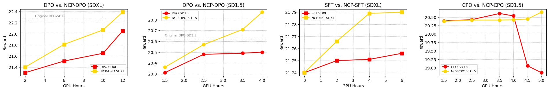
Figure 3: We evaluate the training speed with PickScore on Pick-a-Pic validations set. Our method significantly boosts the learning process compared to baseline methods for DPO and Supervised Fine-Tuning and outperforms their quality. Contrastive Preference Optimization is very unstable due to lack of a reference model. Our method makes it possible to use CPO for tuning Diffusion models.

4 Experiments

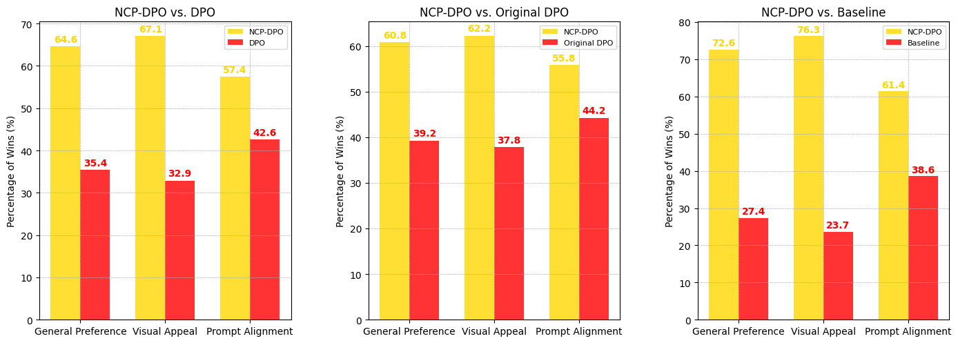
Figure 4: Side-by-side real human preferences comparison for different SDXL models. We compare NCP-DPO with 1) Our own DPO-SDXL 2) Original published DPO-SDXL 3) Baseline model with no preference optimization. Our method significantly improves Direct Preference Optimization. All models are trained on the same data.

In this section we empirically validate our proposed method. Our goal is to show that Noise-Conditioned Perception 1) makes the training procedure much quicker, allowing community to spend much less time and computational resources while getting comparable quality with Diffusion-DPO 2) pushes the boundaries even further and consistently improves the overall quality in terms of manual human preferences.

Setup.

To validate our proposed method we fine-tune Stable Diffusion v1.5 (SD1.5) [27] and Stable Diffusion XL (SDXL) [24] models. We run our largest experiments in terms of compute on a Pick-a-Pic v2 dataset [15], following a setup from [34] that consists of 851,293 pairs, with 58,960 unique prompts, obtained from versions of SDXL and DreamLike (a fine-tune of SD1.5). To validate the speed of learning compared to baseline methods, we filter the dataset, leaving only absolute winners across all prompts and get a version with 87,687 pairs and 53,701 unique prompts. All our checkpoints, including baselines, are obtained with rank 64 LoRA [13] for U-Net weights, contrary to full-finetunes from [34, 17]. We also use 8-bit AdamW optimizer [21] with default hyperparameters and half precision for non-trainable weights everywhere. For all experiments we use learning rate $1e-8\times effective\_batch\_size$ and a warmup exactly like in original Diffusion-DPO paper. All experiments were done using 4x Nvidia H100 GPU and Intel(R) Xeon(R) Platinum 8480+ CPU processor.

Cheaper and Quicker.

To show the efficiency of our proposed method, we use synthetic rewards [35, 15] to evaluate generations during the training process. HPSv2 is considered the most reliable, as it has been shown to correspond best with human judgement. Samples are generated for validation set of Pick-a-Pic-v2 dataset consistins on 500 unique prompts following exactly Diffusion-DPO setup. For each of Supervised Fine-Tuning, DPO, CPO and their corresponding improvements NCP-SFT, NCP-DPO, NCP-CPO we generate images with exactly the same time spent on training. We observe that NCP-DPO-SD1.5 significantly outperforms original DPO-SD1.5 in terms of PickScore reward with only 7.5% of their original steps $\times$ batch size while training only LoRA weights and 8-bit optimizer which reduces the computation many times more. We also note that Contrastive Preference Optimization does not have a reference model that stabilizes training process so the model should tend to overfit and diverge much more. However, NCP-CPO does not have the same effect due to matching trainable U-Net’s embeddings with a frozen copy which adds significant regularization.

Side-by-Side.

To validate the method overall improvements, we follow original Diffusion-DPO paper human feedback annotation setup, comparing generations for PartiPrompts [40] under three different criteria: Q1 General Preference (Which image do you prefer given the prompt?), Q2 Visual Appeal (prompt not considered) (Which image is more visually appealing?) Q3 Prompt Alignment (Which image better fits the text description?). Each generation had 3 independent annotations for each criteria. Image is considered a winner according to a majority votes.

We validate only DPO method. Our human annotations show superior results for both NCP-DPO-SD1.5 and NCP-DPO-SDXL. We compare our largest runs with baseline models, baseline method (DPO) trained by us and original published models. Results are shown in Table 4.

5 Ablation Study

We want to show that by carefully curating the dataset we improve our NCP-DPO over DPO even further. For this purpose, we provide synthetic winrates based on HPSv2 and PickScore. We compare NCP-DPO both on filtered and original Pick-a-Picv2 dataset. The main problem with this dataset lies in contradictory examples across it. A large portion of all images are both winners and losers for some different pairs. Let’s suppose we have three images for one single prompt $x_{1}<x_{2}<x_{3}$ where $<$ denotes preferences. Then, let’s remind a gradient for the Bradley Terry model:

$$\nabla_{\theta}\mathcal{L}_{\mathrm{DPO}}(x^{w},x^{l})=-\beta\mathbb{E}_{(c,x^{w},x^{l})\sim\mathcal{D}}\left[\sigma(r_{\theta}(x^{l})-r_{\theta}(x^{w}))\cdot(\nabla_{\theta}\log p(x^{w})-\nabla_{\theta}\log p(x^{l}))\right]$$ (16)

Now let’s write down the sum of two gradients computed on $x_{1},x_{2}$ and $x_{2},x_{3}$ pairs.

$$\nabla_{\theta}\mathcal{L}_{\mathrm{DPO}}(x_{2},x_{1})+\nabla_{\theta}\mathcal{L}_{\mathrm{DPO}}(x_{3},x_{2}) =-\beta\left[\sigma(r_{\theta}(x_{1})-r_{\theta}(x_{2}))\cdot(\nabla_{\theta}\log p(x_{2})-\nabla_{\theta}\log p(x_{1}))\right]$$ (17)

$$\quad-\beta\left[\sigma(r_{\theta}(x_{2})-r_{\theta}(x_{3}))\cdot(\nabla_{\theta}\log p(x_{3})-\nabla_{\theta}\log p(x_{2}))\right]$$

Notice how terms $\beta\sigma(r_{\theta}(x_{1})-r_{\theta}(x_{2}))\cdot\nabla_{\theta}\log p(x_{2})$ and $\beta\sigma(r_{\theta}(x_{2})-r_{\theta}(x_{3}))\cdot\nabla_{\theta}\log p(x_{2})$ partially cancel each other out, adding noise instead of a clear signal. Excluding contradictory examples, the training process becomes more stable and predictable. Synthetic comparisons for original and filtered dataset are shown in Table 1

NCP-DPO vs DPO	PickScore Winrate	HPSv2 Winrate
SDXL	54.3	55.7
SDXL (filtered data)	65.8	67.1
SD1.5	56.8	59.1
SD1.5 (filtered data)	64.6	71.3

Table 1: Synthetic winrates for NCP-DPO models against DPO. Filtering data improves both NCP-DPO and DPO and makes our method even more powerful.

To further analyze the impact of contradictory examples, we created three additional mini versions of the Pick-a-Pic dataset. For each prompt, we selected their absolute winner $x$ (images that have 0 losses or draws and more than 1 win), their latest losers $y$, and images $z$ that are the latest losers for $y$. Results from Table 2 show that having more losers is important, while winners must be as good as possible.

Comparison	PickScore Median
$x>y$	21.94
$x>y\cup x>z$	21.99
$x>y\cup y>z$	21.95

Table 2: Synthetic PickScore rewards for different dataset setups. $x>y$ stays for mini dataset with absolute winners across all prompts and their latest losers, $x>y\cup y>z$ denotes the same dataset with added images $z$ that are losers to $y$, $x>y\cup x>z$ denotes the same as previous but instead the winners are always absolute. We train these models for 200 steps keeping the same hyperparameters.

6 Discussion

Optimizing Diffusion models for human preferences using Noise-Conditioning Perception is a natural and powerful way to guide the training process of diffusion models. In this work, we have shown that using U-Net’s own encoder embedding space is already a strong baseline for improving both the speed of adaptation to human preferences and the overall quality of the model compared to original methods.

Limitations & Future Work. While Noise-Conditioned Perception works well for diffusion models based on the U-Net architecture, it remains a question for future work whether this approach is applicable to the Diffusion Transformer architecture [23]. We leave this investigation to future research. Additionally, we did not consider cascaded diffusion models [29], an alternative to latent diffusion models like SD, as they are significantly less popular in the open-source community.

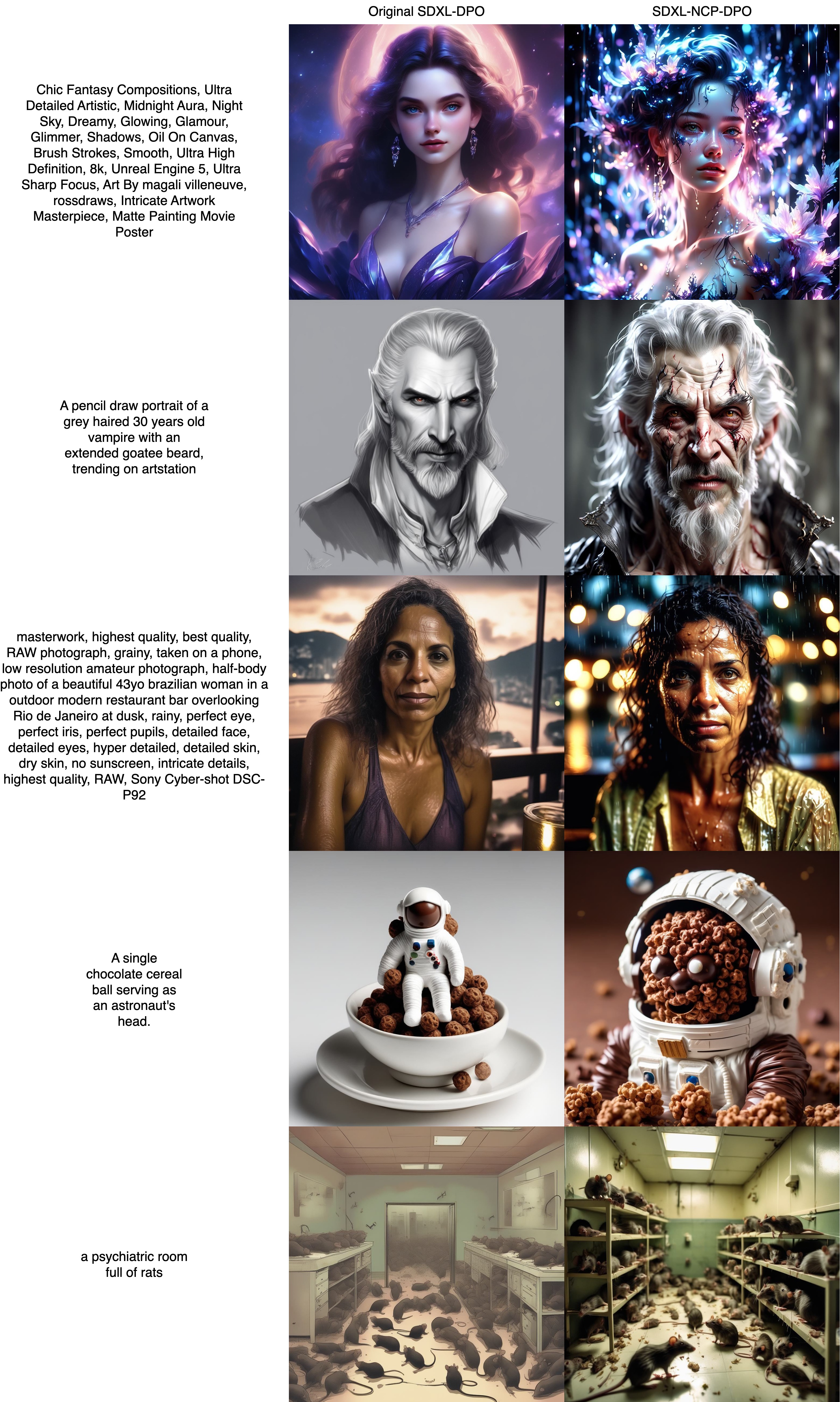
Figure 5: Original Diffusion-DPO and NCP-DPO comparison for Pick-a-Pic validation prompts.

References

- [1] Arpit Bansal, Hong-Min Chu, Avi Schwarzschild, Soumyadip Sengupta, Micah Goldblum, Jonas Geiping, and Tom Goldstein. Universal guidance for diffusion models. In Proceedings of the IEEE/CVF Conference on Computer Vision and Pattern Recognition, pages 843–852, 2023.
- [2] Kevin Black, Michael Janner, Yilun Du, Ilya Kostrikov, and Sergey Levine. Training diffusion models with reinforcement learning. arXiv preprint arXiv:2305.13301, 2023.
- [3] Paul F Christiano, Jan Leike, Tom Brown, Miljan Martic, Shane Legg, and Dario Amodei. Deep reinforcement learning from human preferences. Advances in neural information processing systems, 30, 2017.
- [4] Kevin Clark, Paul Vicol, Kevin Swersky, and David J Fleet. Directly fine-tuning diffusion models on differentiable rewards. arXiv preprint arXiv:2309.17400, 2023.
- [5] Prafulla Dhariwal and Alexander Nichol. Diffusion models beat gans on image synthesis. Advances in neural information processing systems, 34:8780–8794, 2021.
- [6] Dave Epstein, Allan Jabri, Ben Poole, Alexei Efros, and Aleksander Holynski. Diffusion self-guidance for controllable image generation. Advances in Neural Information Processing Systems, 36:16222–16239, 2023.
- [7] Ying Fan, Olivia Watkins, Yuqing Du, Hao Liu, Moonkyung Ryu, Craig Boutilier, Pieter Abbeel, Mohammad Ghavamzadeh, Kangwook Lee, and Kimin Lee. Reinforcement learning for fine-tuning text-to-image diffusion models. Advances in Neural Information Processing Systems, 36, 2024.
- [8] Alexey Gorbatovski, Boris Shaposhnikov, Alexey Malakhov, Nikita Surnachev, Yaroslav Aksenov, Ian Maksimov, Nikita Balagansky, and Daniil Gavrilov. Learn your reference model for real good alignment. arXiv preprint arXiv:2404.09656, 2024.
- [9] Amir Hertz, Ron Mokady, Jay Tenenbaum, Kfir Aberman, Yael Pritch, and Daniel Cohen-Or. Prompt-to-prompt image editing with cross attention control. arXiv preprint arXiv:2208.01626, 2022.
- [10] Jonathan Ho, Ajay Jain, and Pieter Abbeel. Denoising diffusion probabilistic models. Advances in neural information processing systems, 33:6840–6851, 2020.
- [11] Jonathan Ho and Tim Salimans. Classifier-free diffusion guidance. arXiv preprint arXiv:2207.12598, 2022.
- [12] Jiwoo Hong, Noah Lee, and James Thorne. Reference-free monolithic preference optimization with odds ratio. arXiv preprint arXiv:2403.07691, 2024.
- [13] Edward J Hu, Yelong Shen, Phillip Wallis, Zeyuan Allen-Zhu, Yuanzhi Li, Shean Wang, Lu Wang, and Weizhu Chen. Lora: Low-rank adaptation of large language models. arXiv preprint arXiv:2106.09685, 2021.
- [14] Tero Karras, Miika Aittala, Timo Aila, and Samuli Laine. Elucidating the design space of diffusion-based generative models. Advances in Neural Information Processing Systems, 35:26565–26577, 2022.
- [15] Yuval Kirstain, Adam Polyak, Uriel Singer, Shahbuland Matiana, Joe Penna, and Omer Levy. Pick-a-pic: An open dataset of user preferences for text-to-image generation. Advances in Neural Information Processing Systems, 36, 2024.
- [16] Mingi Kwon, Jaeseok Jeong, and Youngjung Uh. Diffusion models already have a semantic latent space. In The Eleventh International Conference on Learning Representations, 2022.
- [17] Shufan Li, Konstantinos Kallidromitis, Akash Gokul, Yusuke Kato, and Kazuki Kozuka. Aligning diffusion models by optimizing human utility. arXiv preprint arXiv:2404.04465, 2024.
- [18] Shanchuan Lin and Xiao Yang. Diffusion model with perceptual loss. arXiv preprint arXiv:2401.00110, 2023.
- [19] Tianqi Liu, Zhen Qin, Junru Wu, Jiaming Shen, Misha Khalman, Rishabh Joshi, Yao Zhao, Mohammad Saleh, Simon Baumgartner, Jialu Liu, et al. Lipo: Listwise preference optimization through learning-to-rank. arXiv preprint arXiv:2402.01878, 2024.
- [20] Tianqi Liu, Yao Zhao, Rishabh Joshi, Misha Khalman, Mohammad Saleh, Peter J Liu, and Jialu Liu. Statistical rejection sampling improves preference optimization. arXiv preprint arXiv:2309.06657, 2023.
- [21] Ilya Loshchilov and Frank Hutter. Decoupled weight decay regularization. arXiv preprint arXiv:1711.05101, 2017.
- [22] Jiajun Ma, Tianyang Hu, Wenjia Wang, and Jiacheng Sun. Elucidating the design space of classifier-guided diffusion generation. In The Twelfth International Conference on Learning Representations, 2023.
- [23] William Peebles and Saining Xie. Scalable diffusion models with transformers. In Proceedings of the IEEE/CVF International Conference on Computer Vision, pages 4195–4205, 2023.
- [24] Dustin Podell, Zion English, Kyle Lacey, Andreas Blattmann, Tim Dockhorn, Jonas Müller, Joe Penna, and Robin Rombach. Sdxl: Improving latent diffusion models for high-resolution image synthesis. arXiv preprint arXiv:2307.01952, 2023.
- [25] Mihir Prabhudesai, Anirudh Goyal, Deepak Pathak, and Katerina Fragkiadaki. Aligning text-to-image diffusion models with reward backpropagation. arXiv preprint arXiv:2310.03739, 2023.
- [26] Rafael Rafailov, Archit Sharma, Eric Mitchell, Christopher D Manning, Stefano Ermon, and Chelsea Finn. Direct preference optimization: Your language model is secretly a reward model. Advances in Neural Information Processing Systems, 36, 2024.
- [27] Robin Rombach, Andreas Blattmann, Dominik Lorenz, Patrick Esser, and Björn Ommer. High-resolution image synthesis with latent diffusion models. In Proceedings of the IEEE/CVF conference on computer vision and pattern recognition, pages 10684–10695, 2022.
- [28] Olaf Ronneberger, Philipp Fischer, and Thomas Brox. U-net: Convolutional networks for biomedical image segmentation. In Medical image computing and computer-assisted intervention–MICCAI 2015: 18th international conference, Munich, Germany, October 5-9, 2015, proceedings, part III 18, pages 234–241. Springer, 2015.
- [29] Chitwan Saharia, William Chan, Saurabh Saxena, Lala Li, Jay Whang, Emily L Denton, Kamyar Ghasemipour, Raphael Gontijo Lopes, Burcu Karagol Ayan, Tim Salimans, et al. Photorealistic text-to-image diffusion models with deep language understanding. Advances in neural information processing systems, 35:36479–36494, 2022.
- [30] John Schulman, Filip Wolski, Prafulla Dhariwal, Alec Radford, and Oleg Klimov. Proximal policy optimization algorithms. arXiv preprint arXiv:1707.06347, 2017.
- [31] Feifan Song, Bowen Yu, Minghao Li, Haiyang Yu, Fei Huang, Yongbin Li, and Houfeng Wang. Preference ranking optimization for human alignment. In Proceedings of the AAAI Conference on Artificial Intelligence, volume 38, pages 18990–18998, 2024.
- [32] Yang Song and Stefano Ermon. Generative modeling by estimating gradients of the data distribution. In H. Wallach, H. Larochelle, A. Beygelzimer, F. d'Alché-Buc, E. Fox, and R. Garnett, editors, Advances in Neural Information Processing Systems, volume 32. Curran Associates, Inc., 2019.
- [33] Fahim Tajwar, Anikait Singh, Archit Sharma, Rafael Rafailov, Jeff Schneider, Tengyang Xie, Stefano Ermon, Chelsea Finn, and Aviral Kumar. Preference fine-tuning of llms should leverage suboptimal, on-policy data. arXiv preprint arXiv:2404.14367, 2024.
- [34] Bram Wallace, Meihua Dang, Rafael Rafailov, Linqi Zhou, Aaron Lou, Senthil Purushwalkam, Stefano Ermon, Caiming Xiong, Shafiq Joty, and Nikhil Naik. Diffusion model alignment using direct preference optimization. arXiv preprint arXiv:2311.12908, 2023.
- [35] Xiaoshi Wu, Yiming Hao, Keqiang Sun, Yixiong Chen, Feng Zhu, Rui Zhao, and Hongsheng Li. Human preference score v2: A solid benchmark for evaluating human preferences of text-to-image synthesis. arXiv preprint arXiv:2306.09341, 2023.
- [36] Weilai Xiang, Hongyu Yang, Di Huang, and Yunhong Wang. Denoising diffusion autoencoders are unified self-supervised learners. In Proceedings of the IEEE/CVF International Conference on Computer Vision (ICCV), pages 15802–15812, October 2023.
- [37] Guangkai Xu, Yongtao Ge, Mingyu Liu, Chengxiang Fan, Kangyang Xie, Zhiyue Zhao, Hao Chen, and Chunhua Shen. Diffusion models trained with large data are transferable visual models. arXiv preprint arXiv:2403.06090, 2024.
- [38] Haoran Xu, Amr Sharaf, Yunmo Chen, Weiting Tan, Lingfeng Shen, Benjamin Van Durme, Kenton Murray, and Young Jin Kim. Contrastive preference optimization: Pushing the boundaries of llm performance in machine translation. arXiv preprint arXiv:2401.08417, 2024.
- [39] Jiazheng Xu, Xiao Liu, Yuchen Wu, Yuxuan Tong, Qinkai Li, Ming Ding, Jie Tang, and Yuxiao Dong. Imagereward: Learning and evaluating human preferences for text-to-image generation. Advances in Neural Information Processing Systems, 36, 2024.
- [40] Jiahui Yu, Yuanzhong Xu, Jing Yu Koh, Thang Luong, Gunjan Baid, Zirui Wang, Vijay Vasudevan, Alexander Ku, Yinfei Yang, Burcu Karagol Ayan, et al. Scaling autoregressive models for content-rich text-to-image generation. arXiv preprint arXiv:2206.10789, 2(3):5, 2022.
- [41] Jiacheng Zhang, Jie Wu, Yuxi Ren, Xin Xia, Huafeng Kuang, Pan Xie, Jiashi Li, Xuefeng Xiao, Weilin Huang, Min Zheng, et al. Unifl: Improve stable diffusion via unified feedback learning. arXiv preprint arXiv:2404.05595, 2024.
- [42] Richard Zhang, Phillip Isola, Alexei A Efros, Eli Shechtman, and Oliver Wang. The unreasonable effectiveness of deep features as a perceptual metric. In Proceedings of the IEEE conference on computer vision and pattern recognition, pages 586–595, 2018.
- [43] Wenliang Zhao, Yongming Rao, Zuyan Liu, Benlin Liu, Jie Zhou, and Jiwen Lu. Unleashing text-to-image diffusion models for visual perception. In Proceedings of the IEEE/CVF International Conference on Computer Vision (ICCV), pages 5729–5739, October 2023.
- [44] Daniel M Ziegler, Nisan Stiennon, Jeffrey Wu, Tom B Brown, Alec Radford, Dario Amodei, Paul Christiano, and Geoffrey Irving. Fine-tuning language models from human preferences. arXiv preprint arXiv:1909.08593, 2019.