Abstract

In a supersymmetric theory, large mass hierarchies can lead to large uncertainties in fixed-order calculations of the Standard Model (SM)-like Higgs mass. A reliable prediction is then obtained by performing the calculation in an effective field theory (EFT) framework, involving a matching to the full supersymmetric theory at the high scale to include contributions from the heavy particles, and a subsequent renormalisation-group running down to the low scale. We report on the prediction of the SM-like Higgs mass within the CP-violating Next-to-Minimal Supersymmetric extension of the SM (NMSSM) in a scenario where all non-SM particles feature TeV-scale masses. The matching conditions are calculated at full one-loop order using two approaches. These are the matching of the quartic Higgs couplings as well as of the SM-like Higgs pole masses of the low- and high-scale theory. A comparison between the two methods allows us to estimate the size of terms suppressed by the heavy mass scale that are neglected in a pure EFT calculation as given by the quartic-coupling matching. Furthermore, we study the different sources of uncertainty which enter our calculation as well as the effect of CP-violating phases on the Higgs mass prediction. The matching calculation is implemented in a new version of the public program package NMSSMCALC.

1 Introduction

Since the discovery of the Standard Model Higgs boson with a mass of about 125 GeV by the ATLAS [1] and the CMS collaboration [2] at the Large Hadron Collider (LHC) at CERN, there has been no clear indication of new degrees of freedom in the range of the weak scale (which can be identified with energy scales around the mass of the W boson, $\sim M_{W}$) to a few TeV scale. Taking into account the constraints from the Higgs data and experimental searches for new degrees of freedom, the parameter space of each Standard Model extension (SM) should be reinvestigated in terms of whether these models can still satisfy the experimental constraints and give possibly detectable new physics signals. Among them, the Minimal Supersymmetric extension of the SM (MSSM) is one of the most studied ones. By imposing a symmetry between bosonic and fermionic degrees of freedom, the particle content is more than doubled with respect to the SM. An interesting feature of this model is related to the Higgs sector. It contains two Higgs doublets due to the requirement of the cancellation of gauge anomalies on the one hand as well as for the generation of non-vanishing masses for all quarks on the other hand. Furthermore, the quartic couplings in the Higgs sector are completely determined by the gauge and Yukawa couplings. As a consequence, the Higgs boson masses can be predicted and one of the Higgs boson masses has an upper limit of about 140 GeV including higher-order corrections [3]. This Higgs boson can be identified with the discovered scalar particle. Similar features occur also in the next-to-MSSM (NMSSM), an extension of the MSSM that includes an extra complex Higgs singlet superfield. However, the upper mass bound can be shifted to higher values due to extra contributions from the Higgs singlet-doublet coupling [4, 5, 6, 7].

Three approaches for the computation of the Higgs boson masses including higher-order corrections have been used. These are the fixed-order (FO), the effective field theory (EFT), and the hybrid technique. For the first one, we have to compute Higgs boson self-energies at fixed loop order and diagonalize the loop-corrected Higgs mass matrix. This calculation involves the full particle spectrum and couplings in the broken phase of the electroweak (EW) symmetry of the model. The corrections will contain terms which are proportional to $y_{x}\ln\tilde{M}_{x}^{2}/M_{x}^{2}$ [3], where $y_{x}$ is the Yukawa coupling, and $M_{x}$ and $\tilde{M}_{x}$ are a masses of an SM particle $x$ and its superpartner, respectively. These terms are particularly important for the top/stop sector, since the top Yukawa coupling is the largest Yukawa coupling. Therefore, if there is large hierarchy between the stop and the top mass the FO calculation breaks down. In such a case, one needs to resum these large logarithms to obtain reliable results. In the EFT calculation, the couplings of the high-energy extension of the SM are matched to the corresponding ones in the effective low-energy field theory such that at the matching scale the physics described by the two models is the same. If only the SM-like particles of the SM extension are light and all the Beyond-SM (BSM) particles are heavy, then the SM is a suitable EFT. In this case, the SM quartic Higgs coupling at the matching scale can be identified with a loop-corrected BSM quartic Higgs coupling at the same scale, which receives only BSM contributions. Therefore, the logarithmic terms are of the form $y_{x}\ln\tilde{M}_{x}^{2}/\mu_{R}^{2}$ where $\mu_{R}$ is the matching scale. Then the logarithmic terms become small when $\tilde{M}_{x}$ is close to $\mu_{R}$. The remaining dependence on $y_{x}\ln\mu_{R}^{2}/M_{x}^{2}$ can be resummed with the help of the SM renormalisation group equations (RGEs) for the Yukawa coupling $y_{x}$. In the literature, there exist two ways to match the loop-corrected BSM quartic Higgs coupling. The first one is called quartic coupling matching which is based on the computation of loop corrections to the four-point vertex using the spectrum and couplings in the limit of the unbroken EW symmetry, $v\to 0$, with $v$ being the vacuum expectation value. The second one is called pole-mass matching which is based on the assumption that also in the BSM theory the SM-like quartic Higgs coupling has a relation with the SM-like Higgs pole mass. By computing the BSM contribution to the SM-like Higgs mass, we can extract information on the quartic Higgs coupling. The computation needs to be done in the broken EW symmetry phase and leads to contributions of ${\cal O}(v^{2}/\tilde{M}_{x}^{2})$. The third approach is called the hybrid technique which combines fixed-order calculations with the EFT approach where the leading and next-to-leading logarithms are resummed and care is taken that no double counting occurs. Therefore, the theory uncertainty at high supersymmetric (SUSY) masses is reduced in comparison to a pure fixed-order result [3]. The gain is two-fold. On the one hand, the theory uncertainty at high supersymmetric (SUSY) masses is reduced in comparison to a pure fixed-order result. On the other hand, finite SUSY mass effects are taken into account in comparison to the pure EFT approach, where they are integrated out.

A lot of effort has been devoted to the precise calculation of the Higgs boson masses in the NMSSM using fixed-order calculations. Leading one-loop, full one-loop and leading two-loop contributions were presented in [8, 9, 10, 11, 12, 13, 14, 15, 16, 17, 18, 19, 20, 21, 22, 23, 24, 25, 26] where the $\overline{\text{DR}}$ renormalisation scheme was applied, except for [18], which also applied a mixed $\overline{\text{DR}}$-on-shell (OS) renormalisation scheme. At two-loop level, all contributions have been computed in the gaugeless limit and using the zero external momentum approximation. The QCD corrections have been discussed in [16] and EW corrections in [27]. Our group has also contributed to the progress of precision predictions for the masses. The full one-loop corrections with momentum dependence were presented in [28, 29] and the two-loop corrections of ${\cal O}{(\alpha_{t}\alpha_{s})}$ in [30], of ${\cal O}(\alpha_{t}^{2})$ in [31], and of ${\cal O}((\alpha_{t}+\alpha_{\lambda}+\alpha_{\kappa})^{2})$ in [32] for both the CP-conserving and the CP-violating NMSSM. We were the first ones to apply a mixed $\overline{\text{DR}}$-OS scheme in the NMSSM with the possibility to choose between either $\overline{\text{DR}}$ or OS conditions in the renormalisation scheme for the top/stop sector. We implemented our FO calculations at one-loop and two-loop ${\cal O}(\alpha_{t}\alpha_{s})$, ${\cal O}(\alpha_{t}^{2})$, and ${\cal O}((\alpha_{t}+\alpha_{\lambda}+\alpha_{\kappa})^{2})$ level in the program package NMSSMCALC [33] which also computes the Higgs boson decay widths and branching ratios both for the CP-conserving and CP-violating case. The code furthermore includes the computation of the loop-corrected trilinear Higgs self-couplings at one-loop [34] and at two-loop ${\cal O}(\alpha_{t}\alpha_{s})$ [35] and ${\cal O}(\alpha_{t}^{2})$ [36] as well as the loop corrections to the $\rho$ parameter and the $W$ boson mass [37]. There are also other public codes such as NMSSMTools [38, 39], SARAH/SPheno [40, 41, 42, 43, 44, 45], SOFTSUSY [46, 47], FlexibleSUSY [48, 49, 49] which are dedicated to the computation of the NMSSM spectrum, decay widths and other observables.

There have been much less activities regarding the EFT approach in the precision Higgs mass calculation in the NMSSM. A discussion of EFT in generic SUSY models including also the NMSSM has been presented in [50]. There the loop-corrected quartic Higgs coupling is obtained from the loop-corrected mass of the lightest Higgs boson after subtracting the corresponding part of the SM. This matching condition has been implemented in FlexibleEFTHiggs and later in SARAH/SPheno [51]. In Ref. [52], the authors have used the matching condition where the loop-corrected quartic Higgs coupling is obtained from the loop-corrected four-point vertex. They have combined a full one-loop computation with the QCD two-loop contributions for the quartic Higgs coupling. This computation has been performed in the limit of the unbroken EW symmetry where the Higgs doublet vacuum expectation values $v_{u},v_{d}\to 0$ while the singlet vacuum expectation value $v_{s}$ is kept non-vanishing and large so that the singlet Higgs masses are very heavy and can then be integrated out.

Our purpose in this paper is threefold. First, we implement both matching conditions discussed in Refs. [50] and [52]. For the pole-mass matching condition we make use of our FO computations of the full one-loop corrections to the Higgs boson masses, which have been implemented in our computer code NMSSMCALC. For this, we modify the renormalisation scheme from the mixed OS-$\overline{\text{DR}}$ to a pure $\overline{\text{DR}}$ scheme for all parameters except the tadpoles for which we still make use of OS-like conditions as in the previously used mixed OS-$\overline{\text{DR}}$ scheme. Using $\overline{\text{DR}}$/$\overline{\text{MS}}$ quantities conveniently enables us to make use of higher-order results in the renormalisation group evolution from the literature. For the four-point vertex matching condition, we compute the full one-loop corrections in the unbroken phase of the EW symmetry in the $\overline{\text{DR}}$ scheme and discuss subtleties related to the $v\to 0$ limit and finite tadpole corrections. We then compare the effect of the two matching methods on the Higgs mass prediction in a large region of the parameter space where the scale of the SUSY particle masses ranges from TeV to hundred TeV. We also compare the EFT approach and the FO calculation in the mixed OS-$\overline{\text{DR}}$ scheme being available in NMSSMCALC where the renormalisation scale is chosen to be the matching scale in the EFT approach. Second, we discuss the effect of the CP-violating phases in the EFT approach which has not been done in the previous publications. Third, we provide an updated version of NMSSMCALC that gives a better treatment in the case where a large mass hierarchy between BSM and SM-like particles occurs.

The paper is organized as follows. In Section 2 we introduce the NMSSM, set up the notation and derive expressions for the tree-level mass matrices and transformations into the mass basis in the limit of a vanishing electroweak VEV. Section 3 discusses the general ingredients for a Higgs mass calculation using an EFT approach. In the first two subsections the pole-mass and quartic-coupling matching approaches are explained in detail while the third subsection describes the estimate of theoretical uncertainties. Section 4 is dedicated to the numerical analysis which validates our results numerically with results from the literature and studies the different EFT approaches and their uncertainties as well as compares to the FO calculation. We conclude in Section 5. The appendix contains the derivation of the tadpole-expansion around a small VEV and details on the implementation in the program NMSSMCALC.

2 The High-Scale NMSSM at Tree-Level

We briefly review the basic ingredients of the complex NMSSM to set up our notation for later use. The model is specified by a scale invariant superpotential $\mathcal{W}_{\text{NMSSM}}$,

$$\mathcal{W}_{\text{NMSSM}}= \left[y_{e}\hat{H}_{d}\!\cdot\!\hat{L}\hat{E}^{c}+y_{d}\hat{H}_{d}\!\cdot\!\hat{Q}\hat{D}^{c}-y_{u}\hat{H}_{u}\hat{Q}\hat{U}^{c}\right]-\lambda\hat{S}\hat{H}_{d}\!\cdot\!\hat{H}_{u}+\frac{1}{3}\kappa\hat{S}^{3}\;,$$ (2.1)

where $\hat{H}_{d}$ and $\hat{H}_{u}$ are the Higgs doublet superfields, $\hat{S}$ the Higgs singlet superfield and $\hat{L}$, $\hat{Q}$, as well as $\hat{E}$, $\hat{D}$, and $\hat{U}$ the left-handed lepton and quark doublet superfields as well as the right-handed lepton, down-type, and up-type quark singlet superfields, respectively. In the following, we will denote the scalar part of the Higgs superfields and the fermion part of the lepton and quark superfields with the same letter without a hat. The lepton, down-type, and up-type quark Yukawa couplings are $y_{e}$, $y_{d}$, $y_{u}$ which are $3\times 3$ matrices that we assume to be diagonal. The summation over generation indices is implicit. The coupling between the Higgs doublet and Higgs singlet superfields is governed by $\lambda$ and the Higgs singlet superfield self-coupling is $\kappa$. Both $\lambda,\kappa$ are considered to be complex parameters with corresponding phases $\varphi_{\lambda},\varphi_{\kappa}$. All Yukawas couplings are taken to be real by rephasing the left- and right-handed Weyl-spinor fields accordingly. The soft-SUSY breaking Lagrangian comprises the soft-SUSY breaking parameters,

$${\cal L}_{\text{soft},\text{ NMSSM}} = -m_{H_{d}}^{2}H_{d}^{\dagger}H_{d}-m_{H_{u}}^{2}H_{u}^{\dagger}H_{u}-m_{\tilde{Q}}^{2}\tilde{Q}^{\dagger}\tilde{Q}-m_{\tilde{L}}^{2}\tilde{L}^{\dagger}\tilde{L}-m_{\tilde{u}_{R}}^{2}\tilde{u}_{R}^{*}\tilde{u}_{R}-m_{\tilde{d}_{R}}^{2}\tilde{d}_{R}^{*}\tilde{d}_{R}$$ (2.2)

$$-m_{\tilde{e}_{R}}^{2}\tilde{e}_{R}^{*}\tilde{e}_{R}-(\epsilon_{ij}[y_{e}A_{e}H_{d}^{i}\tilde{L}^{j}\tilde{e}_{R}^{*}+y_{d}A_{d}H_{d}^{i}\tilde{Q}^{j}\tilde{d}_{R}^{*}-y_{u}A_{u}H_{u}^{i}\tilde{Q}^{j}\tilde{u}_{R}^{*}]+\mathrm{h.c.})$$

$$-\frac{1}{2}(M_{1}\tilde{B}\tilde{B}+M_{2}\tilde{W}_{i}\tilde{W}_{i}+M_{3}\tilde{G}\tilde{G}+\mathrm{h.c.})$$

$$-m_{S}^{2}|S|^{2}+(\epsilon_{ij}\lambda A_{\lambda}SH_{d}^{i}H_{u}^{j}-\frac{1}{3}\kappa A_{\kappa}S^{3}+\mathrm{h.c.})\;,$$

where $\tilde{B}$, $\tilde{W}_{i}$, $\tilde{G}$ are the fermionic $U(1)$ bino, $SU(2)$ wino and $SU(3)$ gluino fields and $A_{e}$, $A_{d}$, $A_{u}$ are the soft-SUSY-breaking trilinear couplings, which are $3\times 3$ matrices and assumed to be diagonal in this paper; again, the summation over the generation indices is implicit here. The soft-SUSY-breaking mass parameters of the sfermions and Higgs fields, $m_{\tilde{Q}}^{2}$, $m_{\tilde{L}}^{2}$, $m_{\tilde{u}_{R}}^{2}$, $m_{\tilde{d}_{R}}^{2}$, $m_{\tilde{e}_{R}}^{2}$, $m_{H_{d}}^{2}$, $m_{H_{u}}^{2}$, and $m_{S}^{2}$ are real and positive while the gaugino masses $M_{1}$, $M_{2}$, $M_{3}$ and the soft SUSY breaking trilinear couplings are complex in general. The scalar Higgs potential is obtained from the superpotential in Eq. (2.1), the soft-SUSY breaking part of the Lagrangian Eq. (2.2) and the $D$ terms originating from the gauge sector of the Lagrangian. Requiring the scalar potential to be minimal at non-vanishing vacuum expectation values (VEVs) of the two Higgs doublets leads to spontaneous breaking of the EW gauge symmetry. Allowing also for the possibility of a singlet VEV, the three Higgs boson fields can be expanded about their VEVs $v_{u}$, $v_{d}$, and $v_{s}$, respectively, as

$$H_{d}=\begin{pmatrix}\frac{v_{d}+h_{d}+ia_{d}}{\sqrt{2}}\\ h_{d}^{-}\end{pmatrix},\,\,H_{u}=e^{i\varphi_{u}}\begin{pmatrix}h_{u}^{+}\\ \frac{v_{u}+h_{u}+ia_{u}}{\sqrt{2}}\end{pmatrix},\,\,S=\frac{e^{i\varphi_{s}}}{\sqrt{2}}(v_{s}+h_{s}+ia_{s})\,,$$ (2.3)

with the CP-violating phases $\varphi_{u,s}$.

For a more comprehensive introduction of the model and its mass spectrum of all sectors at tree-level in the broken phase we refer the reader to our paper [53]. We follow the same convention as in [53].

Since for the quartic coupling matching we need expressions for masses and mixings in the unbroken phase of the EW symmetry, in the following, we present the spectrum of the model in the limit $v_{u},v_{d}\to 0$ but with a fixed ratio of the two VEVs,

$$\tan\beta=\frac{v_{u}}{v_{d}},$$ (2.4)

and a non-vanishing singlet VEV $v_{s}$. We denote the SM-like VEV as $v$, which is related to the two Higgs doublet VEVs as

$$v^{2}=v_{u}^{2}+v_{d}^{2}.$$ (2.5)

Higgs Bosons

In the limit $v\to 0$ the mass matrices of the CP-violating NMSSM take a particularly simple form which allows for an analytical diagonalisation. First, we solve the tadpole equations of $t_{h_{u}},\,t_{h_{d}},\,t_{h_{s}}$ and $t_{a_{d}},\,t_{a_{s}}$ for the soft-SUSY breaking squared masses $m_{{H_{u}}}^{2}$, $m_{{H_{d}}}^{2}$, $m_{S}^{2}$ and the imaginary parts of the parameters $A_{\lambda}$, $A_{\kappa}$, see e.g. Ref. [31]. This is done without taking the limit $v\to 0$ since the solution to the tadpoles may contain terms $\order{v^{-n}}$ which are multiplied with terms $\order{v^{+m}}$ when inserting them into the mass matrices.
Using the tree-level tadpole solutions in the tree-level mass matrices and then performing the limit $v\to 0$, we obtain the following: The squared mass matrix of the charged Higgs boson has one vanishing eigenvalue corresponding to the Goldstone boson and one non-zero eigenvalue corresponding to the physical charged Higgs boson,

$$m_{G^{\pm}}^{2} =0$$ (2.6a)

$$M_{H^{\pm}}^{2} =\frac{|\lambda|(1+\tan^{2}\beta)v_{s}}{2\tan\beta\cos(\varphi_{w}-\varphi_{y})}\left(\sqrt{2}\text{Re}A_{\lambda}+|\kappa|v_{s}\cos\varphi_{w}\right)\;,$$ (2.6b)

where

$$\varphi_{w} = 3\varphi_{s}+\varphi_{\kappa}$$ (2.7)

$$\varphi_{y} = 2\varphi_{s}+\varphi_{\kappa}-\varphi_{\lambda}-\varphi_{u}\;.$$ (2.8)

Thus, we can trade $\text{Re}A_{\lambda}$ for $M_{H^{\pm}}^{2}$. The squared mass matrix for the neutral Higgs bosons takes a block-diagonal form where, after the use of the tadpole solutions, neither the CP-even and the CP-odd components nor the doublet and singlet components mix. The mixing matrix which diagonalizes the neutral Higgs mass matrix transforming the basis $(h_{d},h_{u},h_{s},a_{d},a_{u},a_{s})^{T}$ to the basis $(h,H,S,G^{0},A,A_{s})$, reads

$$\mathcal{R}(\beta)=\left(\begin{array}[]{cc}\mathcal{R}^{H}(\beta)&\textbf{0}\\ \textbf{0}&\mathcal{R}^{G}(\beta)\end{array}\right)$$ (2.9)

with

$$\mathcal{R}^{H}(\beta)=\left(\begin{array}[]{ccc}c_{\beta}&s_{\beta}&0\\ -s_{\beta}&c_{\beta}&0\\ 0&0&1\end{array}\right)\,,\quad\mathcal{R}^{G}(\beta)=\left(\begin{array}[]{ccc}-c_{\beta}&s_{\beta}&0\\ s_{\beta}&c_{\beta}&0\\ 0&0&1\end{array}\right)\,,$$ (2.10)

Diagonalizing the neutral Higgs mass matrix with the help of the mixing matrix in Eq. (2.9) results in a diagonal matrix with the entries

$$m_{h}^{2}(=m_{h_{u}}^{2})= 0\,$$ (2.11a)

$$m_{H}^{2}(=m_{h_{d}}^{2})= M_{H^{\pm}}^{2}$$ (2.11b)

$$m_{S}^{2}\equiv M_{S}^{2}(=m_{h_{s}}^{2})= \frac{|\kappa|v_{s}(4|\kappa|v_{s}+\sqrt{2}\frac{\text{Re}A_{\kappa}}{\cos\varphi_{w}})}{2}\,$$ (2.11c)

$$m_{G^{0}}^{2}(=m_{a_{u}}^{2})= 0\,$$ (2.11d)

$$m_{A}^{2}(=m_{a_{d}}^{2})= M_{H^{\pm}}^{2}\,\,$$ (2.11e)

$$m_{A_{s}}^{2}\equiv M^{2}_{A_{s}}\,(=m_{a_{s}}^{2})= -\frac{3|\kappa|\text{Re}A_{\kappa}v_{s}}{\sqrt{2}\cos\varphi_{w}}\,.$$ (2.11f)

The masses in parenthesis denote the dominant gauge-eigenstates masses. It turns out that for the parameter points that are compatible with all applied constraints and that we discuss in our numerical analysis, the $h$ ($H$) is mostly $h_{u}$-like ($h_{d}$-like) and the $A$ ($G^{0}$) is mostly $a_{d}$-like ($a_{u}$-like). The two vanishing eigenvalues correspond to the neutral Goldstone boson and the SM-like Higgs boson mass. These are the only two neutral scalar states that belong to the EFT, and all remaining heavy neutral Higgs bosons are integrated out. The third eigenvalue $m_{S}^{2}$ corresponds to the mass of the scalar singlet. The second and fifth eigenvalues, $m_{H}^{2}$ and $m_{A}^{2}$, are degenerate and coincide with the mass of the charged Higgs boson, $M_{H^{\pm}}^{2}$. The last eigenvalue, $m_{A_{s}}^{2}$, corresponds to the pseudoscalar singlet. Thus, we can trade the parameters $v_{s}$, $\text{Re}A_{\kappa}$ and $\text{Re}A_{\lambda}$ for $M_{S}$, $M_{A_{s}}$ and $M_{H^{\pm}}$ by inverting Eq. 2.6 and Eq. 2.11.

The set of input parameters which describes the tree-level scalar sector of the NMSSM in case of an unbroken EW symmetry as defined above, at the matching scale then reads:

$$M_{S},\,M_{H^{\pm}},\,M_{A_{s}},\,|\lambda|,\,|\kappa|,\,\tan\beta,\,\varphi_{w},\,\varphi_{y}\;.$$ (2.12)

Fermions

Using the approximation $v\to 0$ the top quark as well as all other SM fermions are massless and do not mix with each other. Considering the fermionic supersymmetric partner particles and assuming the Weyl basis $\psi^{0}=(\tilde{B},\tilde{W}_{3},\tilde{H}^{0}_{d},\tilde{H}^{0}_{u},\tilde{S})^{T}$ and $\psi^{-}=(\tilde{W}^{-},\tilde{H}_{u}^{-})^{T}$ where $\tilde{H}^{0}_{d}$, $\tilde{H}^{0}_{u}$, $\tilde{H}_{u}^{-}$, $\tilde{S}$ are the neutral and charged doublet Higgsino and singlino fields, respectively, for the neutral and the charged fields results in the following neutralino and chargino mass matrices,

$$M_{N}=\begin{pmatrix}M_{1}&0&0&0&0\\ 0&M_{2}&0&0&0\\ 0&0&0&-\lambda\frac{v_{s}}{\sqrt{2}}e^{i\varphi_{s}}&0\\ 0&0&-\lambda\frac{v_{s}}{\sqrt{2}}e^{i\varphi_{s}}&0&0\\ 0&0&0&0&\sqrt{2}\kappa v_{s}e^{i\varphi_{s}}\end{pmatrix}\,,\quad M_{C}=\begin{pmatrix}M_{2}&0\\ 0&\lambda\frac{v_{s}}{\sqrt{2}}e^{i\varphi_{s}}\end{pmatrix}\,.$$ (2.13)

The neutralinos and charginos have a non-zero mass. Their mass-matrices can be diagonalized analytically. We find the following mass eigenvalues:

$$m_{\chi^{0}_{1}} =\lvert M_{1}\rvert$$ (2.14a)

$$m_{\chi^{0}_{2}} =\lvert M_{2}\rvert$$ (2.14b)

$$m_{\chi^{0}_{3}} =m_{\chi^{\pm}_{2}}$$ (2.14c)

$$m_{\chi^{0}_{4}} =m_{\chi^{\pm}_{2}}$$ (2.14d)

$$m_{\chi^{0}_{5}} =\sqrt{\nicefrac{{M_{A_{s}}^{2}}}{{3}}+M_{S}^{2}}$$ (2.14e)

$$m_{\chi^{\pm}_{1}} =\lvert M_{2}\rvert$$ (2.14f)

$$m_{\chi^{\pm}_{2}} =\frac{|\lambda|}{|\kappa|}\frac{\sqrt{\nicefrac{{M_{A_{s}}^{2}}}{{3}}+M_{S}^{2}}}{2}\;,$$ (2.14g)

where all complex phases have been absorbed into the rotation matrices and $v_{s}$ is replaced by

$$v_{s}=\frac{\sqrt{M_{A_{s}}^{2}/3+M_{S}^{2}}}{\sqrt{2}|\kappa|}\;.$$ (2.15)

Sfermions

In the limit $v\to 0$ the squared sfermion mass matrices are only given in terms of the soft-SUSY breaking parameters, and the mixing between left- and right-handed scalars vanishes. Thus their interaction eigenstates coincide with the mass eigenstates,

$$m^{2}_{\tilde{X}}=\left(\begin{array}[]{cc}\bm{m}_{\tilde{X}_{L}}^{2}&0\\ 0&\bm{m}_{\tilde{X}_{R}}^{2}\\ \end{array}\right)\,,\qquad X=u,d,l\,,$$ (2.16)

assuming minimal flavour violation (i.e. diagonal $\bm{m}_{\tilde{X}_{L}}^{2}$, $\bm{m}_{\tilde{X}_{R}}^{2}$). The above diagonal mass matrix has two eigenstates $\tilde{X}_{1,2}$ with masses $m_{\tilde{X}_{1,2}}=\{m_{\tilde{X}_{L}},m_{\tilde{X}_{R}}\}$ for the superpartners of each SM fermion generation. Note that only the 3rd generation of quarks and leptons has significant effects on the Higgs boson masses.

3 The Loop-Corrected Higgs Mass in the EFT Approach

In the scenario that we are considering in this paper, all the soft-SUSY-breaking mass parameters of the sfermions and gauginos, $m_{\tilde{Q}}^{2}$, $m_{\tilde{L}}^{2}$, $m_{\tilde{u}_{R}}^{2}$, $m_{\tilde{d}_{R}}^{2}$, $m_{\tilde{e}_{R}}^{2}$, and $M_{1}$, $M_{2}$, $M_{3}$, together with $M_{S},M_{A_{s}},M_{H^{\pm}}$ are much larger than the SM EW scale. These masses are similar to $\sim M_{\text{\tiny SUSY}}$ where $M_{\text{\tiny SUSY}}\gg v$. Since all SM-like particles have a mass $m_{\text{\tiny SM}}\propto v$, this means $M_{\text{\tiny SUSY}}\gg m_{\text{\tiny SM}}$.

In such a scenario, a fixed-order approach will lead to large logarithms of $\ln(v^{2}/M_{\text{\tiny SUSY}}^{2})$ which will destroy the perturbative expansion and hence a precise prediction. Therefore, we follow the EFT approach where we match the NMSSM to the effective field theory (that we identify with the SM in this paper) at the scale $M_{\text{\tiny SUSY}}$ in such a way that at $M_{\text{\tiny SUSY}}$ both theories lead to the same physical predictions. The contributions containing large logarithms of $\ln(v^{2}/M_{\text{\tiny SUSY}}^{2})$ will be resummed through the SM renormalisation group equations (RGE). In the NMSSM calculation, we will denote the SM-like Higgs that is matched to the Higgs boson of the EFT as the one which is predominantly made up of the $h_{u}$ component of Eq. (2.3).

For the matching procedure, we are following two matching condition schemes which allow us to relate the effective quartic Higgs coupling $\lambda_{h}^{\text{SM}}$ in the SM to the one in the NMSSM. For the quartic interaction term we use the normalisation $-\lambda_{h}^{\text{SM}}|H|^{4}$, with the neutral component of the SM Higgs doublet $H$ given by $H^{0}=\frac{1}{\sqrt{2}}(v^{\text{SM}}+h+iG^{0})$.

• In the first scheme, we directly require the four-point functions, i.e. matrix elements, with four external Higgs bosons in the SM and the SM-like Higgs bosons in the NMSSM to be the same at the matching scale. We can then calculate loop corrections to the quartic Higgs coupling within the NMSSM, $\lambda_{h}^{\text{NMSSM}}$, that we then identify with the loop-corrected SM one $\lambda_{h}^{\text{SM}}$. In the following, we will refer to this scheme as quartic-coupling matching.

• In the second scheme, we demand that the pole masses of the Higgs boson in the SM and the SM-like Higgs boson in the NMSSM are equal at the matching scale. The SM $\overline{\text{MS}}$ mass at the matching scale is then computed from this matching condition. Here, it has to be ensured that all large logarithms of $\ln(v^{2}/M_{\text{\tiny SUSY}}^{2})$ are canceled by applying a proper expansion. The extraction of the effective quartic Higgs coupling via Eq. (3.45) is discussed in Sec. 3.2 in more detail. We will refer to this scheme as pole-mass matching.

The major difference between the two matching schemes consists in the diagrams to be evaluated (cf. [54] for a detailed discussion): While the quartic-coupling matching requires four-point functions to be calculated in the limit of $v\to 0$, the pole-mass matching requires at most only two-point functions, i.e. self energies, to be evaluated, at the expense of having to carry out the calculation in the EW-broken phase and then expanding systematically in $v^{2}/M_{\text{\tiny SUSY}}^{2}$. In both matching schemes, we obtain a value for the effective quartic Higgs coupling of the SM, capturing the effects of the heavy particles with masses $\sim M_{\text{\tiny SUSY}}$ and resumming all large logarithms $\ln(v^{2}/M_{\text{\tiny SUSY}}^{2})$ consistently via RGEs. Before presenting the calculation of the effective quartic Higgs couplings in the two matching schemes, we show in Fig. 1 our procedure for the computation of the loop-corrected Higgs mass in the EFT approach, implemented in the new version of NMSSMCALC, and describe it in detail in the following.

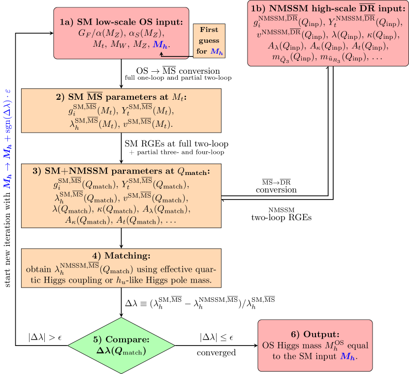
Figure 1: Schematic procedure for the computation of the loop-corrected Higgs mass in the EFT approach implemented in NMSSMCALC.

We start with the six SM input parameters (box 1a of Fig. 1) which can be either

$$G_{F},~{}\alpha_{S}(M_{Z}),~{}M_{t},~{}M_{W},~{}M_{Z},~{}M_{h}$$ (3.17)

or

$$\alpha(M_{Z}),~{}\alpha_{S}(M_{Z}),~{}M_{t},~{}M_{W},~{}M_{Z},~{}M_{h},$$ (3.18)

where all masses are considered to be the pole masses. We call the choice of input parameters of Eq. (3.17) the “$G_{F}$ scheme”, while we denote the choice of Eq. (3.18) as the “$\alpha_{M_{Z}}$ scheme”. We then have to convert all OS input parameters to their corresponding $\overline{\text{MS}}$ parameters at the scale $M_{t}$. For the $\alpha_{M_{Z}}$ scheme we use the conversion formulae which are already available in NMSSMCALC. These conversion formulae have been given in the appendix D of [31], but we use them now at the scale $M_{t}$ instead of $M_{Z}$. For the $G_{F}$ scheme, we use the conversion formulae at the scale $M_{t}$, presented in [55].

As running $\overline{\text{MS}}$ parameters in the SM, we choose (box 2)

$$g_{1}^{\text{SM},\,\overline{\text{MS}}},~{}g_{2}^{\text{SM},\,\overline{\text{MS}}},~{}g_{3}^{\text{SM},\,\overline{\text{MS}}},~{}Y_{t}^{\text{SM},\,\overline{\text{MS}}},~{}v^{\text{SM},\,\overline{\text{MS}}},~{}\lambda_{h}^{\text{SM},\,\overline{\text{MS}}}\,.$$ (3.19)

As usual, we denote by $g_{1}$, $g_{2}$, $g_{3}$ the three gauge couplings of the corresponding three gauge symmetry groups $U(1)_{Y}$, $SU(2)_{L}$ and $SU(3)_{C}$, while $Y_{t}$ is the top Yukawa coupling. After obtaining these $\overline{\text{MS}}$ parameters at $M_{t}$, we apply the SM RGEs including full two-loop and partial three- and four-loop contributions [41, 56, 57, 58] to run up to the matching scale which is denoted by $Q_{\text{match}}$ with $Q_{\text{match}}\gg M_{t}$.

For the NMSSM calculation at the high-energy scale $Q_{\text{inp}}$ (box 1b), we have the following input parameters:

$$v_{s},~{}\tan\beta,~{}m_{\tilde{Q}_{3}},~{}m_{\tilde{u}_{R_{3}}},~{}M_{1},~{}M_{2},~{}M_{3},~{}\lambda,~{}\kappa,~{}A_{t},~{}\mbox{Re}A_{\lambda},~{}\mbox{Re}A_{\kappa},~{}\varphi_{u},~{}\varphi_{s}$$ (3.20)

as well as the corresponding parameters of Eq. (3.19) in the $\overline{\text{DR}}$ scheme with the exception of the quartic Higgs coupling $\lambda_{h}$, which is not an input parameter in the NMSSM. We remind that the $M_{1,2,3}$ and $A_{t}$ are complex, their phases are included in the running from $Q_{\text{inp}}$ to $Q_{\text{match}}$, while the imaginary parts of $A_{\lambda}$ and $A_{\kappa}$ are eliminated through the tadpole equations at $Q_{\text{match}}$. Note, that for the sfermion contributions we only take into account corrections from the stops, i.e. the top-quark Yukawa coupling is the only non-zero Yukawa coupling. In order to relate the high-scale parameters $g_{i}^{{\text{NMSSM}},\overline{\text{DR}}}$, $Y_{t}^{{\text{NMSSM}},\overline{\text{DR}}}$, $v^{{\text{NMSSM}},\overline{\text{DR}}}$ to the ones at the low scale and thus express our calculations in the NMSSM solely via the low-scale $\overline{\text{MS}}$ parameters, we first evolve them from the high-energy input scale $Q_{\text{inp}}$ to the matching scale $Q_{\text{match}}$ using two-loop RGEs in the NMSSM and then perform a matching at the scale $Q_{\text{match}}$. The $\overline{\text{MS}}\to\overline{\text{DR}}$ conversion formulae for $g_{1}$, $g_{2}$ and $g_{3}$ between high-scale and low-scale parameters at 1-loop level are given by

$$g_{i}^{{\text{NMSSM}},\overline{\text{DR}}}=g_{i}^{{\text{SM}},\overline{\text{MS}}}+\delta g_{i}^{\text{reg}}+\delta g_{i}^{\text{thr}}\,,$$ (3.21)

where the $\delta g_{i}^{\text{reg}}$ denote $\overline{\text{MS}}$–$\overline{\text{DR}}$ shifts related to the difference in the regularization schemes [59],

$$\delta g_{1}^{\text{reg}}=0\,,\qquad\delta g_{2}^{\text{reg}}=\frac{g_{2}^{3}}{48\pi^{2}}\,,\qquad\delta g_{3}^{\text{reg}}=\frac{g_{3}^{3}}{32\pi^{2}}\,,$$ (3.22)

and the $\delta g_{i}^{\text{thr}}$ are the threshold corrections for $v\to 0$ including the effects of the heavy particles which are integrated out in the EFT [61]. They read

$$\begin{split}\delta g_{1}^{\text{thr}}&=-\frac{g_{1}^{3}}{512\pi^{2}}\left[12\ln\frac{\mu_{\text{eff}}^{2}}{Q^{2}}+3\ln\frac{M_{H^{\pm}}^{2}}{Q^{2}}+\sum_{i=3}\left(3\ln\frac{m_{\tilde{L}_{i}}^{2}}{Q^{2}}+6\ln\frac{m_{\tilde{e}_{R,i}}^{2}}{Q^{2}}\right)\right.\\ &\qquad\qquad\qquad\left.{}+\sum_{i=1}^{3}\left(\ln\frac{m_{\tilde{Q}_{i}}^{2}}{Q^{2}}+8\ln\frac{m_{\tilde{u}_{R,i}}^{2}}{Q^{2}}+2\ln\frac{m_{\tilde{d}_{R,i}}^{2}}{Q^{2}}\right)\right],\end{split}$$ (3.23)

$$\delta g_{2}^{\text{thr}} =-\frac{g_{2}^{3}}{192\pi^{2}}\left[8\ln\frac{M_{2}^{2}}{Q^{2}}+4\ln\frac{\mu_{\text{eff}}^{2}}{Q^{2}}+\ln\frac{M_{H^{\pm}}^{2}}{Q^{2}}+\sum_{i=3}\left(\ln\frac{m_{\tilde{L}_{i}}^{2}}{Q^{2}}+3\ln\frac{m_{\tilde{Q}_{i}}^{2}}{Q^{2}}\right)\right],$$ (3.24)

$$\delta g_{3}^{\text{thr}} =-\frac{g_{3}^{3}}{192\pi^{2}}\left[12\ln\frac{M_{3}^{2}}{Q^{2}}+\sum_{i=1}^{3}\left(2\ln\frac{m_{\tilde{Q}_{i}}^{2}}{Q^{2}}+\ln\frac{m_{\tilde{u}_{R,i}}^{2}}{Q^{2}}+\ln\frac{m_{\tilde{d}_{R,i}}^{2}}{Q^{2}}\right)\right],$$ (3.25)

where $Q=Q_{\text{match}}$, and we introduced the effective $\mu$ parameter,

$$\mu_{\text{eff}}=\lambda\frac{v_{s}}{\sqrt{2}}e^{i\varphi_{s}},$$ (3.26)

and $M_{H^{\pm}}^{2}$ is given in Eq. (2.6). For the top Yukawa coupling, we only require the matching relation at tree level for a consistent calculation of the effective quartic Higgs coupling at 1-loop order,

$$Y_{t}^{{\text{NMSSM}},\overline{\text{DR}}}=Y_{t}^{{\text{SM}},\overline{\text{MS}}}/\sin\beta.$$ (3.27)

The matching of the VEV will be discussed in Sec. 3.2, as it is not needed for the quartic coupling matching in the unbroken phase, but for the pole mass matching. With the NMSSM $\overline{\text{DR}}$ parameters $g_{i}^{{\text{NMSSM}},\overline{\text{DR}}}$, $Y_{i}^{{\text{NMSSM}},\overline{\text{DR}}}$, expressed through their low-scale $\overline{\text{MS}}$ counterparts, and the other SUSY input parameters of Eq. (3.20) at the scale $Q_{\text{match}}\sim M_{\text{\tiny SUSY}}$ (box 3), we can then compute the loop corrections in the NMSSM to the quartic Higgs coupling $\lambda_{h}^{{{\text{NMSSM}},\overline{\text{MS}}}}(Q_{\text{match}})$ of the $h_{u}$-like Higgs boson, or to the pole mass of the $h_{u}$-like Higgs boson, subtracting the SM corrections consistently and keeping only the pure NMSSM contributions (box 4).

Note that in our implementation, we allow the matching scale $Q_{\text{match}}$ to be different from the input scale $Q_{\text{inp}}$ at which the SUSY parameters of Eq. (3.20) are given. In the case of $Q_{\text{match}}\neq Q_{\text{inp}}$, we use the two-loop NMSSM RGEs as calculated by SARAH [40, 41, 42, 43, 62, 63, 64, 65, 66] to run the SUSY parameters from $Q_{\text{inp}}$ to $Q_{\text{match}}$. As the Yukawa and gauge couplings are given at $Q_{\text{match}}$ (and not $Q_{\text{inp}}$) via their low-scale inputs, we thus have to implement the running of the SUSY parameters via an iterative procedure until all parameters converge at the matching scale. We note that due to the RGE running, a CP-violating phase of one of the soft-SUSY-breaking parameters typically induces CP-violating phases also for the other SUSY parameters, so that the CP-violating effects cannot be limited to only one sector of the model.

The obtained loop-corrected $\lambda_{h}^{{{\text{NMSSM}},\overline{\text{MS}}}}(Q_{\text{match}})$ is then compared to the quartic Higgs coupling of the SM $\lambda_{h}^{{{\text{SM}},\overline{\text{MS}}}}(Q_{\text{match}})$ of Eq. (3.19) at the scale $Q_{\text{match}}$ (box 5). If the absolute value of the relative difference between the two quartic couplings, $\Delta\lambda\equiv(\lambda^{{\text{SM}},\overline{\text{MS}}}-\lambda^{{\text{NMSSM}},\overline{\text{MS}}})/\lambda^{{\text{SM}},\overline{\text{MS}}}$, is larger than $\epsilon=10^{-5}$, we change the SM input $M_{h}$ and, starting again from the top of Fig. 1, iterate the procedure until the precision goal $|\Delta\lambda|<\epsilon$ is reached. In order to efficiently scan over different values of $M_{h}$, we use the bisection method for which the procedure converges in logarithmic time. The found value of $M_{h}$ for which the SM and NMSSM quartic Higgs couplings have the same value at the matching scale $Q_{\text{match}}$ (within the precision goal) and at the considered loop order is then identified with our predicted loop-corrected SM-like on-shell Higgs mass in the EFT approach (box 6).

To compare the two approaches for the matching conditions, in the numerical discussion in Sec. 4, we will denote the obtained values for the SM-like on-shell Higgs mass by $M_{h}^{\text{\tiny\Romanbar{4}}}$ for the quartic-coupling matching and by $M_{h}^{\text{\tiny\Romanbar{2}}}$ for the pole-mass matching, i.e. the Roman superscript specifies which scalar $n$-point function was used in the matching.

3.1 Quartic-Coupling Matching Conditions

We present here our computation of the effective quartic Higgs coupling at the tree and one-loop level after subtracting the SM contributions, i.e. the contributions from all particles which appear in the SM EFT Lagrangian. To improve our prediction, we have included two-loop QCD and mixed QCD-EW corrections in the limit of the CP-conserving MSSM which are available in SUSYHD [67] and Ref. [68], respectively. Our $\lambda_{h}^{{{\text{NMSSM}},\overline{\text{MS}}}}(Q_{\text{match}})$ can then be written as the sum of the tree-level, one-loop, and MSSM two-loop parts,

$$\lambda_{h}^{{{\text{NMSSM}},\overline{\text{MS}}}}(Q_{\text{match}})=\lambda_{h}^{{\text{NMSSM}},\text{tree}}+\Delta\lambda_{h}^{{\text{NMSSM}},\text{1l}}+\Delta\lambda_{h}^{\text{MSSM},\text{2l}}\,.$$ (3.28)

Note, that $\Delta\lambda_{h}^{\text{MSSM},\text{2l}}$ is not sensitive to the CP-violating phases entering $\lambda_{h}^{{\text{NMSSM}},\text{tree}}$ and $\Delta\lambda_{h}^{{\text{NMSSM}},\text{1l}}$.

3.1.1 Tree Level

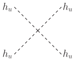
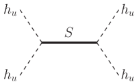
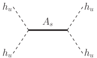
Figure 2: Exemplary tree-level diagrams which contribute to the tree-level quartic-coupling matching. Thick (thin) lines denote heavy (light) particles which are (not) integrated out in the EFT. The dashed external lines correspond to the SM-like ($h_{u}$-like) Higgs eigenstate. The second and third diagrams exhibiting a heavy CP-even ($S$) or CP-odd ($A_{s}$) singlet in the propagator have to be taken into account also for $t$- and $u$-channel propagators. Note that the third diagram with the $A_{s}$ exchange is absent in the CP-conserving case.

At the tree-level the four-$h_{u}$ vertex gets contribution from the Feynman diagrams sketched in Fig. 2. Taking into account all tree-level contributions to the effective quartic Higgs coupling, we get the following expression,

$$\lambda_{h}^{{\text{NMSSM}},\text{tree}} =\underbrace{\frac{1}{8}(g_{1}^{2}+g_{2}^{2})\cos^{2}2\beta}_{\text{MSSM $D$-terms}}{}~{}\,+{}\underbrace{\frac{1}{4}|\lambda|^{2}\sin^{2}2\beta}_{\text{NMSSM $F$-terms}}$$ (3.29a)

$$\begin{split}&\quad{}-\frac{1}{48|\kappa|^{2}M_{S}^{2}(3M_{S}^{2}+M_{A_{s}}^{2})}\Bigg{(}3|\kappa|^{2}M_{H^{\pm}}^{2}\left(1-\cos 4\beta\right)\\ &\quad\underbrace{\qquad\qquad\qquad\qquad\quad{}+(3M_{S}^{2}+M_{A_{s}}^{2})\left(|\kappa||\lambda|\cos\varphi_{y}\sin 2\beta-2|\lambda|^{2}\right)\Bigg{)}^{2}}_{\text{$s$/$t$/$u$-channel $S$}}\end{split}$$ (3.29b)

$$\quad{}\underbrace{-\frac{3}{16M_{A_{s}}^{2}}|\lambda|^{2}(3M_{S}^{2}+M_{A_{s}}^{2})\sin^{2}2\beta\sin^{2}\varphi_{y}}_{\text{$s$/$t$/$u$-channel $A_{s}$}}\,,$$ (3.29c)

where the origin of each term is explained by the corresponding text underneath. While the two contributions of Eq. (3.29a) directly originate from the scalar potential in the NMSSM, the terms of Eqs. (3.29b) and (3.29c) arise when the heavy CP-even and CP-odd singlets, appearing as intermediate states in the $s$-, $t$-, and $u$-channels, are integrated out. Note that the charged Higgs boson does not contribute at tree level and the appearance of $M_{H^{\pm}}$ in Eq. (3.29b) is only related to our choice of parametrization to replace the real part of $A_{\lambda}$ in favor of the input parameter $M_{H^{\pm}}$. Compared to the CP-conserving case presented in [52], there are additional contributions from the CP-odd singlet field $A_{s}$, corresponding to the term in Eq. (3.29c). This term will vanish if $\sin\varphi_{y}=0$, i.e. if there is no CP-violation at tree-level in the Higgs sector.

3.1.2 One Loop

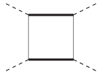
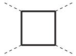
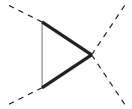
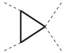
a)	b)	c)	d)
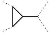
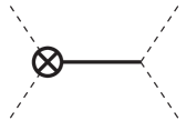
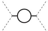
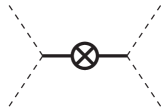
e)	f)	g)	h)

Figure 3: Selection of one-loop diagrams contributing to the one-loop quartic-coupling matching. Thick (thin) lines denote heavy (light) particles which are (not) integrated out in the EFT. The diagrams a)-e) and g) show exemplary box, vertex correction and self-energy diagrams, while the diagrams f) and h) represent the vertex and mass counterterm diagrams, which implicitly contain contributions from tadpoles.

At the one-loop level, the matching condition of the quartic Higgs coupling receives corrections from diagrams involving at least one heavy SUSY particle. In Fig. 3 we show example diagrams, where thick lines correspond to heavy SUSY particles and thin lines to light SM fields. We divide the one-loop corrections into the following six pieces,

$$\Delta\lambda_{h}^{{\text{NMSSM}},\text{1l}}=\Delta\lambda_{\Box}+\Delta\lambda_{\triangle}+\Delta\lambda_{\rm SE}+\Delta\lambda_{\rm CT}+\Delta\lambda_{\text{reg}}+\Delta\lambda_{\text{gauge-thr}}\,.$$ (3.30)

The first four terms correspond to the box, vertex correction, self-energy and counterterm contributions, respectively. The last two terms correspond to the shift induced by the different regularization schemes used in the NMSSM and the SM calculations and the contributions from the matching of the gauge couplings. In all above contributions, diagrams with only SM particles (light states) in the internal lines are discarded, since they belong to the SM contributions and would cancel in the matching condition. All diagrams which contain at least one SUSY particles (heavy state) in the internal lines are kept. Since the momenta of the external Higgs bosons are set to be zero, all four-, three- and two-point one-loop integrals can be be reduced to vacuum integrals. For the calculation of the diagrams we make use of the mass- and mixing-matrices of the NMSSM in the unbroken phase of the EW symmetry as specified in Section 2.

Box diagrams such as shown in Fig. 3 a) to d) are of similar structure as those which are encountered in the MSSM with the difference that the additional NMSSM degrees-of-freedom are present in the loop. They constitute a separately UV-finite subset. An entirely new type of correction arises in the (complex) NMSSM due to the presence of the non-local contributions at tree-level, cf. Fig. 2 b) and c). At the one-loop level, these diagrams receive vertex corrections $\Delta\lambda_{\triangle}$, propagator corrections $\Delta\lambda_{\text{SE}}$, and corresponding counterterm corrections $\Delta\lambda_{\text{CT}}$ shown exemplary in Fig. 3 e) to h). The vertex corrections originate from the exchanges of a CP-even or a CP-odd singlet which can be written as

$$\Delta\lambda_{\triangle}=-\frac{1}{2}\frac{g_{hhS}}{M_{S}^{2}}\Delta g_{hhS}-\frac{1}{2}\frac{g_{hhA_{s}}}{M_{A_{s}}^{2}}\Delta g_{hhA_{s}}$$ (3.31)

where $\Delta g_{hhS},\Delta g_{hhA_{s}}$ are genuine one-loop contributions to the triple Higgs vertices $h-h-S$ and $h-h-A_{s}$, respectively, and the trilinear couplings $g_{hhS},g_{hhA_{s}}$ are given in Eq. (3.35a) and Eq. (3.35b), respectively. The factor of $1/2$ comes from our normalisation of the quartic coupling. The propagator corrections come from the one-loop self-energy diagrams of the heavy CP-even and CP-odd singlet states. They can be expressed as

$$\Delta\lambda_{\rm SE}=\frac{1}{2}\left(\frac{g_{hhS}}{M_{S}^{2}}\right)^{2}\Sigma_{SS}(0)+\frac{1}{2}\left(\frac{g_{hhA_{s}}}{M_{A_{s}}^{2}}\right)^{2}\Sigma_{A_{s}A_{s}}(0)+\frac{g_{hhA_{s}}g_{hhS}}{M_{A_{s}}^{2}M_{S}^{2}}\Sigma_{SA_{s}}(0)$$ (3.32)

where $\Sigma_{xy}(0)$ ($x,y=S,A_{s}$) are the self-energies of the transitions $x\to y$ evaluated at zero external momentum in the limit $v\to 0$. For the counterterm contributions, we note that all parameters appearing in the tree-level expression in Eq. (3.29c) are renormalised in the $\overline{\text{DR}}$ scheme except for those parameters, which are treated for OS tadpoles. As a consequence, the counterterm of $\lambda_{h}^{{\text{NMSSM}}}$ gets UV-finite contributions only from the wave-function renormalisation constant of the external Higgs fields, the singlet tadpoles and the tadpole of the field $a_{d}$. The latter enters via the counterterm of $\text{Im}(A_{\lambda})$. We can express $\Delta\lambda_{\rm CT}$ as

$$\ \Delta\lambda_{\rm CT} =2\lambda_{h}^{{\text{NMSSM}},\text{tree}}\delta^{(1)}Z_{h}-\frac{\delta^{(1)}t_{h_{s}}}{2v_{s}}\left(\frac{g_{hhS}^{2}}{M_{S}^{2}}+\frac{g_{hhA_{s}}^{2}}{M_{A_{s}}^{2}}\right)$$

$$+\frac{\delta^{(1)}t_{a_{s}}}{2v_{s}}\left(3\frac{g_{hhA_{s}}^{2}}{M_{A_{s}}^{2}}\tan\varphi_{w}-2\frac{g_{hhA_{s}}g_{hhS}}{M_{A_{s}}^{2}M_{S}^{2}}-\frac{g_{hhS}^{2}}{M_{S}^{2}}\tan\varphi_{w}\right)$$

$$\left.+\delta^{(1)}\text{Im}(A_{\lambda})\left(\frac{g_{hh{A_{s}}}}{M_{A_{s}}^{2}}\frac{\partial g_{hh{A_{s}}}}{\partial\text{Im}(A_{\lambda})}+\frac{g_{hhS}}{M_{S}^{2}}\frac{\partial g_{hhS}}{\partial\text{Im}(A_{\lambda})}\right)\right|_{\text{min}}$$ (3.33)

where the tadpole counterterms $\delta^{(1)}t_{h_{s},a_{s}}$ originate from mass-counterterm inserted diagrams, Fig. 3 h), and $\delta^{(1)}\text{Im}A_{\lambda}$ from the vertex-counterterm inserted diagrams in Fig. 3 f). The subscript ’min’ indicates that the expression is evaluated at the minimum of the potential (where Im$(A_{\lambda})$ is no input anymore), i.e. using the solutions for the tadpole equations. The Higgs field wave-function renormalisation constant at one-loop order is given by

$$\delta^{(1)}Z_{h}=-\frac{d\Sigma_{hh}}{dp^{2}}\bigg{|}_{p^{2}=0}$$ (3.34)

and the trilinear Higgs couplings related to the singlet states as well as their partial derivatives w.r.t. to $\text{Im}(A_{\lambda})$ are

$$g_{hhS} =\frac{1}{2v_{s}}\left(|\kappa||\lambda|v_{s}^{2}\sin(2\beta)\cos\varphi_{y}-2|\lambda|^{2}v_{s}^{2}+M_{H^{\pm}}^{2}\sin^{2}(2\beta)\right)\,,$$ (3.35a)

$$g_{hhA_{S}} =-\frac{3}{2}|\kappa||\lambda|v_{s}\sin(2\beta)\sin\varphi_{y}\,,$$ (3.35b)

$$\frac{\partial g_{hhS}}{\partial\text{Im}(A_{\lambda})} =-|\lambda|\sin(2\beta)\sin(\varphi_{w}-\varphi_{y})\,,$$ (3.35c)

$$\frac{\partial g_{hhA_{S}}}{\partial\text{Im}(A_{\lambda})} =-|\lambda|\sin(2\beta)\cos(\varphi_{w}-\varphi_{y})\,.$$ (3.35d)

All other counterterm diagrams are of $\mathcal{O}(v^{2}/M_{\text{\tiny SUSY}}^{2})$ or higher and neglected in the quartic coupling matching. Note, that the couplings in Eq. 3.35a-Eq. 3.35d are given at the minimum of the tree-level potential while the derivatives of the couplings have to be evaluated before using the tadpole solutions. Finally, the counterterm of $\text{Im}(A_{\lambda})$ is related to the counterterm of the $a_{d}$-tadpole via the tree-level tadpole solution as

$$\delta^{(1)}\text{Im}(A_{\lambda})=\frac{\sqrt{2}}{|\lambda|v_{s}\cos(\varphi_{w}-\varphi_{y})\sin\beta}\frac{\delta^{(1)}t_{a_{d}}}{v}\,.$$ (3.36)

The above contributions have been obtained by two independent calculations. One calculation relies on SARAH [69] to compute the expression for the effective quartic Higgs self-coupling and the other one uses FeynArts-3.11 [70, 71] and FeynCalc-9.3 [72, 73, 74]. Note that in [52], the authors found that in the old version of SARAH, a term related to the singlet tadpole was missing. After implementing generic tadpoles into a private version of SARAH and computing the singlet tadpole contributions, the results from the two calculations were found to agree.

At the beginning of this section, we discussed that the quartic-coupling matching is performed in the limit of the unbroken phase, $v\to 0$. This is also the general strategy employed in [60, 69]. However, from Eq. 3.36 we can see, that the actual limit $v\to 0$ has to be taken with care in the CP-violating case and requires the expansion of tadpoles up to $\mathcal{O}(v)$. The explicit expansion of $\delta^{(1)}t_{a_{d}}/v$ up to $\mathcal{O}((v^{2}/M_{\text{\tiny SUSY}}^{2})^{0})$ is derived in Appendix A. It should be stressed, that this situation was not encountered before in e.g. calculations within the CP-violating MSSM: In the MSSM all diagrams that contain $\delta^{(1)}t_{i}/v$-terms are suppressed by additional powers of $v$.

Finally, we have to take into account the shift due to the NMSSM calculation being done in the $\overline{\text{DR}}$ scheme and the SM contributions being calculated in the $\overline{\text{MS}}$ scheme,

$$\Delta\lambda_{\text{reg}}=\frac{1}{64\pi^{2}}\left[\frac{g_{2}^{4}}{3}\cos^{2}2\beta-\frac{1}{2}\left(g_{1}^{4}+2g_{1}^{2}g_{2}^{2}+3g_{2}^{4}\right)\right].$$ (3.37)

There are two contributions to this shift: The first term in Eq. (3.37) accounts for the $\overline{\text{DR}}$–$\overline{\text{MS}}$ conversion of the gauge couplings given in Eq. (3.22), since we express all gauge and Yukawa parameters in the threshold corrections to the quartic coupling in Eq. (3.30) by their $\overline{\text{MS}}$ values of the low-energy EFT. An additional contribution arises due to diagrams involving quartic couplings between two Higgs and two gauge bosons [69]. As explained above, we discard all diagrams containing only SM-fields i.e. we implicitly subtract these pieces in the $\overline{\text{DR}}$ scheme. However, the subtraction-term strictly would need to be computed in the $\overline{\text{MS}}$ scheme using dimensional regularization rather than dimensional reduction. The second term of Eq. (3.37) remedies this mismatch between the two schemes in the subtracted SM contributions.

In addition to the regularisation-scheme shift to the gauge couplings, we also take into account the one-loop gauge thresholds from the matching of the gauge couplings between the NMSSM and the SM,

$$\Delta\lambda_{\text{gauge-thr}} =\lambda^{{\text{NMSSM}},\text{tree}}_{h}(g_{i}\to g_{i}+\delta g_{i}^{\text{thr}})-\lambda^{{\text{NMSSM}},\text{tree}}_{h}(g_{i})$$

$$=\frac{1}{4}\left(g_{1}\delta g_{1}^{\text{thr}}+g_{2}\delta g_{2}^{\text{thr}}\right)\cos^{2}2\beta\,+\order{(\delta g_{i})^{2}},$$ (3.38)

that arise when integrating out all heavy degrees of freedom of the NMSSM. The $\delta g_{i}^{\text{thr}}$ are defined in Eqs. (3.23) and (3.24). As the singlet states in the NMSSM do not influence the gauge couplings, the shifts of Eqs. (3.37) and (3.38) are identical to the ones of the MSSM [61].

3.2 Pole-Mass Matching Conditions

The pole-mass matching scheme is defined by the condition that the pole-mass of the SM-like Higgs mass eigenstate in the NMSSM is equal to the SM one,

$$(M_{h}^{\text{SM}})^{2}\stackrel{{\scriptstyle!}}{{=}}(M_{h}^{\text{NMSSM}})^{2}\,.$$ (3.39)

The defining equation for the pole-mass in the SM reads

$$0=p^{2}-(m_{h}^{\text{SM}})^{2}+\mbox{Re}\hat{\Sigma}_{h}^{\text{SM}}(p^{2}=(M_{h}^{\text{SM}})^{2})\,.$$ (3.40)

Here, $m_{h}^{\text{SM}}$ denotes the running $\overline{\text{MS}}$ mass of the SM Higgs boson, i.e. the tree-level mass expressed through $\overline{\text{MS}}$ parameters, and $\hat{\Sigma}_{h}^{\text{SM}}$ is the renormalised one-loop self-energy calculated at a fixed order in the $\overline{\text{MS}}$ renormalisation scheme. The solution $p^{2}=(M_{h}^{\text{SM}})^{2}$, which fulfills Eq. 3.40 in general has to be found iteratively. The calculation of the pole mass of the SM-like Higgs boson in the NMSSM on the right-hand side of Eq. (3.39) is more complicated due to the appearance of multiple Higgs states and their mixing. In general, the pole masses of the Higgs bosons in the NMSSM are the eigenvalues of the loop-corrected Higgs mass matrix $\mathcal{M}_{H}$,

$$\big{(}\mathcal{M}_{H}\big{)}_{ij}=(m_{h_{i}}^{\text{NMSSM}})^{2}\delta_{ij}-\mbox{Re}\hat{\Sigma}_{ij}^{\text{NMSSM}}(p^{2})\qquad\text{for }i,j=1,\ldots,5\,,$$ (3.41)

where $m_{h_{i}}^{\text{NMSSM}}$ is the tree-level mass of $h_{i}$ (expressed through the running $\overline{\text{DR}}$ parameters). In NMSSMCALC, the squared tree-level masses are obtained after factorizing the Goldstone boson and then diagonalizing the tree-level mass matrix. The eigenvalues are the squared masses that are ordered by ascending mass values. The $\hat{\Sigma}_{ij}^{\text{NMSSM}}(p^{2})$ in Eq. (3.41) denote the $\overline{\text{DR}}$-renormalised self-energies of the transitions $h_{i}\to h_{j}$ at the momentum squared $p^{2}$. Similarly to the SM, we take only the real part of the renormalised self-energy for our following discussions. The $i$th loop-corrected pole mass, $(M_{h_{i}}^{\text{NMSSM}})^{2}$, is then obtained by iteratively diagonalizing the mass matrix $\mathcal{M}_{H}$ until $p^{2}$ approaches $(M_{h_{i}}^{\text{NMSSM}})^{2}$. However, both the diagonalisation of the loop-corrected mass matrix and the iterative procedure mix different orders of perturbation theory. This mixing can spoil the cancellation of large logarithms by inducing higher powers of $\ln(v^{2}/M_{\text{\tiny SUSY}}^{2})$-terms. Thus, an iterative procedure may induce a large theory uncertainty.

In order to obtain a consistent one-loop expansion which is free of any powers of $\ln(v^{2}/M_{\text{\tiny SUSY}}^{2})$, we approximate the loop-corrected SM-like Higgs pole mass: We work in the tree-level mass basis as in Eq. (3.41). In the following, we assume that the SM-like Higgs state always corresponds to $h_{1}$ with the tree-level mass $m_{h}^{\text{NMSSM}}\equiv m_{h_{1}}^{\text{NMSSM}}$,

$$(M_{h}^{\text{NMSSM}})^{2}\equiv\big{(}\mathcal{M}_{H}\big{)}_{11}=(m_{h}^{\text{NMSSM}})^{2}-\mbox{Re}\hat{\Sigma}_{11}^{\text{NMSSM}}\big{(}p^{2}\big{)}\,,$$ (3.42)

i.e. we consider only the diagonal element corresponding to the lightest state. At the one-loop level, it is consistent to ignore all mixing self-energy contributions since the diagonalisation of the loop-corrected mass matrix only involves terms proportional to the product of two or more one-loop self-energies. In order to avoid further mixing of orders in the iteration, we take only the first iteration of the pole-mass equation where the momentum squared is set to be equal to the tree-level mass squared, $(M_{h}^{X})^{2}=(m_{h}^{X})^{2}-\mbox{Re}\hat{\Sigma}_{h}^{X}(p^{2}=(m_{h}^{X})^{2})$ for $X=\{{\text{SM}},{\text{NMSSM}}\}$. The matching of the pole-masses in the two theories, Eqs. 3.40 and 3.42, is then performed successively: We first evaluate the matching condition at the tree-level which yields $(m_{h}^{\text{SM}})^{2}=(m_{h}^{\text{NMSSM}})^{2}$. Using this in the one-loop matching condition, Eq. 3.39, we find

$$(m_{h}^{\text{SM}})^{2}-\mbox{Re}\hat{\Sigma}_{h}^{\text{SM}}\big{(}(m_{h}^{\text{NMSSM}})^{2}\big{)}\stackrel{{\scriptstyle!}}{{=}}(m_{h}^{\text{NMSSM}})^{2}-\mbox{Re}\hat{\Sigma}_{h}^{\text{NMSSM}}\big{(}(m_{h}^{\text{NMSSM}})^{2}\big{)}\,,$$ (3.43)

where we write $\hat{\Sigma}_{h}^{\text{NMSSM}}\equiv\hat{\Sigma}_{11}^{\text{NMSSM}}$ to simplify the notation. For a consistent expansion of the matching condition in $v^{2}/M_{\text{\tiny SUSY}}^{2}$, the real part of the self-energies can then furthermore be expanded around small arguments,

$$\mbox{Re}\hat{\Sigma}_{h}^{X}\big{(}(m_{h}^{\text{NMSSM}})^{2}\big{)}=\hat{\Sigma}_{h}^{X}(0)+(m_{h}^{\text{NMSSM}})^{2}\,\hat{\Sigma}^{X\prime}_{h}(0)+\mathcal{O}\big{(}(m_{h}^{\text{NMSSM}})^{4}\big{)}\,.$$ (3.44)

Using the expansion of Eq. (3.44) in Eq. (3.43), the large logarithms $\ln(M_{\text{\tiny SUSY}}/v)$ at the matching scale $Q_{\text{match}}\sim M_{\text{\tiny SUSY}}$ are the same on the left- and right-hand sides, and the matching condition as a whole is thus free of these logarithms. We finally note that, contrary to e.g. [50], no explicit tadpole contributions are appearing in Eq. (3.43), as we define the minimum of our scalar potential to correspond to the tree-level one at all orders (“on-shell tadpole scheme”). Thus, the tadpole contributions are taken into account implicitly via the mass-matrix counterterm included in the renormalised self-energies (see e.g. Appendix G of [31], with all counterterms, other than the ones for the tadpoles, set to zero due to the $\overline{\text{MS}}/\overline{\text{DR}}$ scheme used in our calculation).

The tree-level relation between the $\overline{\text{MS}}$ mass $m_{h}^{\text{SM}}$ and the quartic coupling parameter of the SM Lagrangian in the $\overline{\text{MS}}$ scheme reads

$$(m_{h}^{\text{SM}})^{2}=2(v^{\text{SM}})^{2}\,\lambda_{h}^{{\text{SM}},{\text{\tiny\Romanbar{2}}}}\,,$$ (3.45)

where $v^{\text{SM}}$ is the VEV of the SM in the $\overline{\text{MS}}$ scheme. Using this relation, Eq. (3.43) implicitly defines a matching condition for the quartic coupling and therefore allows to extract a prediction for the effective quartic coupling of the SM-like Higgs in the NMSSM at the matching scale, which we will denote for consistency with the above notation as $\lambda_{h}^{{{\text{NMSSM}},\overline{\text{MS}}},{\text{\tiny\Romanbar{2}}}}$. Contrary to the quartic-coupling matching, the appearance of the VEV in Eq. (3.45) prevents us from setting $v\to 0$ right from the beginning. The pole-mass matching thus requires a double expansion in the loop order as well as in $v^{2}/M_{\text{\tiny SUSY}}^{2}$. Solving Eq. (3.43) for the quartic coupling appearing in Eq. (3.45), the pole-mass matching condition can then be cast in a similar form as the quartic-coupling matching:

$$\lambda_{h}^{{{\text{NMSSM}},\overline{\text{MS}}},{\text{\tiny\Romanbar{2}}}}=\lambda_{h}^{{\text{NMSSM}},\text{tree},{\text{\tiny\Romanbar{2}}}}+\Delta\lambda_{h}^{{\text{NMSSM}},\text{1l},{\text{\tiny\Romanbar{2}}}}+\Delta\lambda_{h}^{\text{MSSM},\text{2l}}\,,$$ (3.46)

where we again improve our result by adding the two-loop MSSM corrections of [67] as in the case of the quartic-coupling matching in Eq. (3.28). We introduce the additional superscript 2 in order to distinguish the effective quartic coupling obtained via the pole-mass matching approach from the corresponding one of the quartic-coupling matching approach in Eq. (3.28), since the former includes also partial $v^{2}/M_{\text{\tiny SUSY}}^{2}$ terms.

The pole mass obtained in the NMSSM depends on the VEV as defined in the high-energy theory, $v^{\text{NMSSM}}$. As we want to express the matching condition only in terms of either $v^{\text{NMSSM}}$ or $v^{\text{SM}}$, it is thus also required to match the VEV and take into account the shift between the two,

$$(v^{\text{SM}})^{2}=(v^{\text{NMSSM}})^{2}+\delta v^{2}=(v^{\text{NMSSM}})^{2}\left(1+\frac{\delta v^{2}}{v^{2}}\right)\,.$$ (3.47)

In the last term of Eq. (3.47), we do not distinguish between $v^{\text{SM}}$ and $v^{\text{NMSSM}}$, as the difference is of higher order. The threshold correction $\delta v^{2}$ can be obtained from matching e.g. the $Z$-boson pole mass at one loop in the SM and the NMSSM, which can then futhermore be related through Ward identities to the wave-function renormalisation of the Higgs boson [60],

$$\frac{\delta v^{2}}{v^{2}}=\left[\hat{\Sigma}^{{\text{NMSSM}}\prime}_{h}(0)-\hat{\Sigma}^{{\text{SM}}\prime}_{h}(0)\right]+\mathcal{O}(v^{2}/M_{\text{\tiny SUSY}}^{2})\,,$$ (3.48)

where $\hat{\Sigma}^{X\prime}_{h}$ denotes the first derivative of the self energy with respect to the four-momentum squared.

Analogously to the quartic-coupling matching, we express the gauge and Yukawa couplings entering the NMSSM self-energies in terms of the $\overline{\text{MS}}$ quantities of the low-energy effective theory. Thus, we use a tree-level matching of the Yukawa couplings due to their appearance only starting from one loop, and the one-loop matching for the gauge couplings of Eq. (3.21). If we were to simply plug in Eq. (3.21) into the tree-level mass term $(m_{h}^{\text{NMSSM}})^{2}$ of Eq. (3.43), we would induce partial two-loop contributions and higher (possibly spoiling the cancellation of large logarithms). In order to include the gauge shifts consistently at the one-loop order, we expand the tree-level mass in $\delta g_{i}=\delta g_{i}^{\text{reg}}+\delta g_{i}^{\text{thr}}$ ($i=1,2$) to first order

$$\left(m_{h}^{{\text{NMSSM}}}\right)^{2} \equiv\left(m_{h}^{\text{NMSSM}}(g_{i}^{{{\text{NMSSM}},\overline{\text{DR}}}}\to g_{i}^{{{\text{SM}},\overline{\text{MS}}}}+\delta g_{i})\right)^{2}$$

$$=\left(m_{h}^{{\text{NMSSM}},\text{tree}}(g_{i}^{{{\text{SM}},\overline{\text{MS}}}})\right)^{2}+\delta^{\text{gauge}}m_{h}^{2}+\order{(\delta g_{i})^{2}}$$ (3.49)

The pole-mass matching involves a rotation into the mass basis,

$$\delta^{\text{gauge}}m_{h}^{2} =\left(\mathcal{R}^{H}(v)\delta^{\text{gauge}}\bm{M}_{H}\mathcal{R}^{H^{T}}(v)\right)_{11}\,,$$ (3.50)

where $\mathcal{R}^{H}(v)$ are the rotation matrices that diagonalise the squared neutral Higgs mass matrix, $\mathcal{R}^{H}(v)\bm{M}_{H}\mathcal{R}^{H^{T}}(v)=(m_{h_{i}}^{{\text{NMSSM}}})^{2}\delta_{ij}$, in the broken phase (i.e. not as in Eq. 2.10 but for the case of non-zero $v$) and

$$\delta^{\text{gauge}}\bm{M}_{H}=\sum_{i=1,2}\left.(\delta g_{i}^{\text{thr}}+\delta g_{i}^{\text{reg}})\frac{\partial}{\partial g_{i}^{{{\text{NMSSM}},\overline{\text{DR}}}}}\bm{M}_{H}\right|_{g_{i}^{{{\text{NMSSM}},\overline{\text{DR}}}}\to g_{i}^{{{\text{SM}},\overline{\text{MS}}}}}\,.$$ (3.51)

With this treatment we guarantee that all logarithms of the form $\ln v/Q_{\text{match}}$ appearing in the electroweak corrections can cancel in the pole-mass matching while we still correctly take into account the leading corrections from the $\overline{\text{DR}}-\overline{\text{MS}}$ conversion. However, in the numerical analysis we found that these effect are numerically small compared to e.g. the stop contributions.

3.2.1 Tree Level

Keeping only the lowest-order terms of Eq. (3.43) and setting the self-energy corrections to zero, we obtain together with Eq. (3.45) the condition

$$(m_{h}^{\text{SM}})^{2}=2(v^{\text{SM}})^{2}\,\lambda_{h}^{{\text{SM}},{\text{\tiny\Romanbar{2}}}}\stackrel{{\scriptstyle!}}{{=}}(m_{h}^{\text{NMSSM}})^{2}\,.$$ (3.52)

At lowest order, we do not have to take into account the threshold corrections to the VEV, so we can set $v^{\text{SM}}=v^{\text{NMSSM}}$ with $\delta v^{2}=0$. Furthermore, the right-hand side of Eq. (3.52) is expressed via the SUSY and the low-energy $\overline{\text{MS}}$ gauge parameters only, so that we also set $\delta m^{2}_{h,\text{gauge}}$ of Eq. (3.50) to zero. Equation (3.52) thus becomes the tree-level matching relation for the effective quartic coupling:

$$\lambda_{h}^{{\text{SM}},{\text{\tiny\Romanbar{2}}}}\stackrel{{\scriptstyle!}}{{=}}\frac{(m_{h}^{\text{NMSSM}})^{2}}{2(v^{\text{NMSSM}})^{2}}\equiv\lambda_{h}^{{\text{NMSSM}},\text{tree},{\text{\tiny\Romanbar{2}}}}.$$ (3.53)

We have checked that, by analytically diagonalizing the tree-level Higgs mass matrix in the NMSSM with full VEV dependence to obtain $m_{h}^{\text{NMSSM}}$ and then expanding Eq. (3.53) in $v^{2}/M_{\text{\tiny SUSY}}^{2}$, the same expression as in Eqs. (3.29a)–(3.29c) is obtained at the lowest order $\mathcal{O}((v^{2}/M_{\text{\tiny SUSY}}^{2})^{0})$.

3.2.2 One Loop

At one-loop order, we take into account the one-loop self energies in Eq. (3.43), and obtain after plugging in Eq. (3.45):

$$2(v^{\text{SM}})^{2}\,\lambda_{h}^{{\text{SM}},{\text{\tiny\Romanbar{2}}}}-\hat{\Sigma}_{h}^{\text{SM}}\big{(}(m_{h}^{\text{NMSSM}})^{2}\big{)}\stackrel{{\scriptstyle!}}{{=}}(m_{h}^{\text{NMSSM}})^{2}-\hat{\Sigma}_{h}^{\text{NMSSM}}\big{(}(m_{h}^{\text{NMSSM}})^{2}\big{)}\,,$$ (3.54)

which results in the expression for the effective quartic coupling:

$$\begin{split}\lambda_{h}^{{\text{SM}},{\text{\tiny\Romanbar{2}}}}&\stackrel{{\scriptstyle!}}{{=}}\frac{1}{2(v^{\text{SM}})^{2}}\left[(m_{h}^{\text{NMSSM}})^{2}-\hat{\Sigma}_{h}^{\text{NMSSM}}\big{(}(m_{h}^{\text{NMSSM}})^{2}\big{)}+\hat{\Sigma}_{h}^{\text{SM}}\big{(}(m_{h}^{\text{NMSSM}})^{2}\big{)}\right]\\ &\equiv\lambda_{h}^{{\text{NMSSM}},\text{tree},{\text{\tiny\Romanbar{2}}}}+\Delta\lambda_{h}^{{\text{NMSSM}},\text{1l},{\text{\tiny\Romanbar{2}}}}\,.\end{split}$$ (3.55)

To extract the leading terms in the expansion of $v^{2}/M_{\text{\tiny SUSY}}^{2}$, we replace $v^{\text{SM}}$ by $v^{\text{NMSSM}}$ according to Eqs. (3.47) and (3.48), and we expand the self-energies according to Eq. (3.44), so that eventually, we obtain for the one-loop contribution to the matching condition:

$$\Delta\lambda_{h}^{{\text{NMSSM}},\text{1l},{\text{\tiny\Romanbar{2}}}}=-\frac{1}{2(v^{\text{NMSSM}})^{2}}\left[\Delta\hat{\Sigma}_{h}+2(m_{h}^{\text{NMSSM}})^{2}\Delta\hat{\Sigma}^{\prime}_{h}\right],$$ (3.56)

where we have introduced the abbreviation $\Delta\hat{\Sigma}^{(\prime)}_{h}\equiv\hat{\Sigma}^{{\text{NMSSM}}(\prime)}_{h}(0)-\hat{\Sigma}^{{\text{SM}}(\prime)}_{h}(0)$. The last term of Eq. (3.56) can for $v\to 0$ immediately be identified with the first term of Eq. (3.33), corresponding to the wave-function-renormalisation contribution. In the tree-level piece of Eq. (3.55), given via Eq. (3.53), we apply the replacement of Eq. (3.50) in order to take into account the $\overline{\text{DR}}$-$\overline{\text{MS}}$ and gauge threshold shifts consistently at the one-loop order. Then, Eq. (3.55) is again expressed through the SUSY input parameters as well as the $\overline{\text{MS}}$ parameters of the low-energy theory only.

The self-energies and wave-function renormalisation contributions required for the calculation of the pole-mass matching at one loop are identical to the ones used for fixed-order calculations of the pole masses, and we can therefore reuse the available expressions in the NMSSMCALC code after modifying the counterterms such that the self-energies, which are given in the code in a mixed on-shell–$\overline{\text{DR}}$ scheme, are renormalised purely in the $\overline{\text{DR}}$ scheme.

As the pole-mass matching procedure depends non-trivially on the value of the VEV due to the tree-level mass diagonalisation, and relies on numerical cancellations between different terms, the VEV cannot be set to zero exactly, and the suppressed $v^{2}/M_{\text{\tiny SUSY}}^{2}$ terms are thus always included. As a cross check of the consistent one-loop implementation of the pole-mass matching procedure, we have numerically evaluated the matching procedure for an artificially small value of $v\sim 1$ GeV to decrease the size of the $v^{2}/M_{\text{\tiny SUSY}}^{2}$ terms, and found in general very good agreement with the quartic-coupling matching approach of Sec. 3.1, see the discussion in Sec. 4.5.2.

Finally, we also include two-loop MSSM corrections [67, 68] to the matching condition, see Eq. (3.46). However, unlike the one-loop results obtained with the pole-mass matching, the two-loop results are not sensitive to $v^{2}/M_{\text{\tiny SUSY}}^{2}$ terms or CP-violating phases.

3.3 Uncertainty Estimate

In this section we describe the method used to estimate different theoretical uncertainties entering the Higgs mass prediction. For a review of commonly considered uncertainties see e.g. Ref. [7]. It is useful to distinguish between two sources of uncertainty which originate in relations used at the low-energy electroweak scale (SM uncertainty) and at the high-energy matching scale (SUSY uncertainty).

SM uncertainties:

The low-energy uncertainty contains different components:

• Missing electroweak corrections in the extraction of SM $\overline{\text{MS}}$ parameters are estimated by choosing either the Fermi constant $G_{F}$ or the fine structure constant $\alpha_{M_{Z}}$ as an input and adapting the renormalisation of the electroweak sector accordingly using either the $G_{F}$-scheme [37] or the $\alpha_{M_{Z}}$-scheme [32]. We denote the difference in the Higgs mass prediction between the two renormalisation schemes by

  $$\Delta^{{\text{SM}}}_{G_{F}/\alpha_{M_{Z}}}=\lvert M_{h}^{G_{F}}-M_{h}^{\alpha_{M_{Z}}}\rvert.$$ (3.57)

• To estimate missing higher-order corrections in the relation between $\lambda^{{\text{SM}},\,\overline{\text{MS}}}$ and the Higgs pole-mass beyond the gauge-less limit, we take the $\overline{\text{MS}}$ parameters (obtained in step 2 of Fig. 1), run them to $Q_{\text{EW}}=M_{t}/2$ and $2M_{t}$, respectively, using SM RGEs and compute the Higgs pole-mass at the two-loop order in the $\overline{\text{MS}}$ scheme by solving

  $$0=p^{2}-2\lambda_{h}^{{{\text{SM}},\overline{\text{MS}}}}(Q_{\text{EW}})v^{2}(Q_{\text{EW}})+\mathrm{Re}\Sigma_{h}(p^{2},Q_{\text{EW}})|_{\mathrm{UV-fin}}$$ (3.58)

  iteratively for $p^{2}=M_{h}^{\overline{\text{MS}}\mathrm{,pole}}(Q_{\text{EW}})$. In Eq. 3.58 we evaluate the UV-finite part of the Higgs self-energy in the $\overline{\text{MS}}$ scheme at the full one-loop level and take into account the leading two-loop $\order{\alpha_{t}(\alpha_{t}+\alpha_{s})}$ corrections, obtained with FeynCalc and TARCER. As a reference point we use the OS Higgs pole-mass from step 1a and estimate the uncertainty as

  $$\Delta^{{\text{SM}}}_{Q_{\rm EW}}=\max\{\lvert M_{h}^{\mathrm{OS}}-M_{h}^{\overline{\mathrm{MS}}\mathrm{,pole}}(2M_{t})\rvert,\lvert M_{h}^{\mathrm{OS}}-M_{h}^{\overline{\mathrm{MS}}\mathrm{,pole}}(M_{t}/2)\rvert\}.$$ (3.59)

  Since these shifts are not symmetric around $M_{t}$, we take the maximum of the two differences. The estimate is performed for a fixed electroweak scheme which can be chosen in the SLHA input file ($\alpha_{M_{Z}}$ or $G_{F}$).

• The third component computes the Higgs boson mass while adding/removing three-loop (and higher-order) corrections to the $\overline{\text{MS}}$ top quark Yukawa coupling:

  $$\Delta^{{\text{SM}}}_{Y_{t}}=M_{h}({Y_{t}^{\order{\alpha_{s}^{2}}}})-M_{h}({Y_{t}^{\order{\alpha_{s}^{3}}}}).$$ (3.60)

  This shift has been obtained numerically using the code mr for $m_{h}=125.1\,\mathrm{GeV}$ and $M_{t}=172.76\,\mathrm{GeV}$. The three-loop shift is negative and typically causes a decrease of the effective SM Higgs mass of about $\sim$800 MeV.

It should be noted that the three types of uncertainties are not completely independent from each other with the exception of $\Delta^{{\text{SM}}}_{G_{F}/\alpha_{M_{Z}}}$ and $\Delta^{{\text{SM}}}_{Y_{t}}$, which can be considered to be independent.

SUSY uncertainties:

For the estimate of the high-scale uncertainty, we generated the two-loop RGEs for the CP-violating NMSSM using SARAH and implemented them in NMSSMCALC. As stated before, the matching scale and the SUSY scale (defining the scale of the SUSY $\overline{\text{DR}}$ input parameters) do not need to be the same. We change the matching scale in the range of $[M_{\text{\tiny SUSY}}/2,2M_{\text{\tiny SUSY}}]$, and then compare to the result obtained with $Q_{\text{match}}=M_{\text{\tiny SUSY}}$. It should be noted that these shifts are not symmetric around $Q_{\rm match}=M_{\text{\tiny SUSY}}$ and therefore we take the maximum of the two differences as

$$\Delta^{\rm SUSY}_{Q_{\rm match}}=\max\{\lvert M_{h}^{M_{\text{\tiny SUSY}}/2}-M_{h}^{M_{\text{\tiny SUSY}}}\rvert,\lvert M_{h}^{2M_{\text{\tiny SUSY}}}-M_{h}^{M_{\text{\tiny SUSY}}}\rvert\}.$$ (3.61)

To estimate the uncertainty of missing higher-order corrections to the matching condition which are not scale-dependent, one typically changes the definition of the top-quark Yukawa coupling entering the matching condition. The structure of the NMSSM-specific component of this type of uncertainty was already discussed in Ref. [52]. Since we plan to include exactly this type of missing higher-order corrections via a pole-mass matching using the results of Ref. [32] in the near future, we also leave the corresponding uncertainty estimate for future work.

Combined uncertainty:

The total uncertainty is computed by assuming independent individual uncertainties,

$$\Delta M_{h}^{\text{\tiny\Romanbar{2}}}=\left[\left(\Delta^{\rm SM}_{G_{F}/\alpha_{M_{Z}}}\right)^{2}+\left(\Delta^{\rm SM}_{Q_{\rm EW}}\right)^{2}+\left(\Delta^{\rm SM}_{Y_{t}}\right)^{2}+\left(\Delta^{\rm SUSY}_{Q_{\rm match}}\right)^{2}\right]^{\frac{1}{2}}\,.$$ (3.62)

As stated above, not all uncertainties are independent of each other. Therefore, the total uncertainty computed by NMSSMCALC is a rather conservative estimate. Equation (3.62) is used to estimate the uncertainty of the Higgs mass prediction if the pole-mass matching was chosen in the SLHA input. If the quartic coupling matching was chosen, the uncertainty is given by

$$\Delta M_{h}^{\text{\tiny\Romanbar{4}}}=\Big{[}\left(\Delta M_{h}^{\text{\tiny\Romanbar{2}}}\right)^{2}+(\underbrace{M_{h}^{\text{\tiny\Romanbar{2}}}-M_{h}^{\text{\tiny\Romanbar{4}}}}_{\equiv\Delta^{\rm SUSY}_{v^{2}/M_{\text{\tiny SUSY}}^{2}}})^{2}\Big{]}^{\frac{1}{2}}\,,$$ (3.63)

which takes the missing $\nicefrac{{v^{2}}}{{M_{\text{\tiny SUSY}}^{2}}}$-terms into account and is labeled as a third uncertainty, the EFT uncertainty $\Delta^{\rm SUSY}_{v^{2}/M_{\text{\tiny SUSY}}^{2}}$, in Ref. [7].

4 Numerical Results

In this section we investigate the results for the SM-like Higgs boson mass prediction numerically using the implementation in NMSSMCALC. We first perform a numerical cross-check of our result by comparing with the findings of Ref. [52]. Furthermore, we investigate the size of the $\nicefrac{{v^{2}}}{{M_{\text{\tiny SUSY}}^{2}}}$ corrections in different corners of the parameter space by comparing results obtained with either the pole-mass or quartic-coupling matching and investigate the size of the individual uncertainty components. Finally we also discuss the effects of CP-violating phases on the Higgs mass prediction.

4.1 Setup and Applied Constraints

The physical SM input parameters used in step 1a of Fig. 1 are

$$\begin{array}[]{lcllcl}G_{F}&=&1.1663788\times 10^{-5}\,~{}\text{GeV}^{-2},&\quad\alpha(M_{Z})&=&1/127.955\,,\\ \alpha_{s}(M_{Z})&=&0.1181\,,&\quad M_{t}&=&172.69\,~{}\text{GeV}\,,\\ m_{b}^{\overline{\text{MS}}}&=&4.18\,~{}\text{GeV}\,,&\quad M_{\tau}&=&1.77682\,~{}\text{GeV}\,,\\ M_{W}&=&80.377\,~{}\text{GeV}\,,&\quad M_{Z}&=&91.1876\,~{}\text{GeV}\,,\end{array}$$ (4.68)

where either $G_{F}$ or $\alpha_{M_{Z}}$ is used as an input depending on the renormalisation scheme choice, cf. Section 3.

In order to investigate the difference between the two matching procedures and the FO calculation (in the $\overline{\text{DR}}$ scheme) and to assess the reliability of each calculation in different corners of the NMSSM parameter space, we have performed a parameter scan varying the NMSSM input parameters uniformly in the following ranges,

$$100\,\mathrm{GeV}\leq M_{1},M_{2}\leq 1.5\,\mathrm{TeV}, \qquad 100\,\mathrm{GeV}\leq\mu_{\text{eff}}\leq 1.5\,\mathrm{TeV},$$

$$1\,\mathrm{TeV}\leq m_{\tilde{Q}_{L_{3}}},m_{\tilde{t}_{R_{3}}}\leq 2.5\,\mathrm{TeV}, \qquad M_{\text{\tiny SUSY}}=\sqrt{m_{\tilde{Q}_{L_{3}}}m_{\tilde{t}_{R_{3}}}},$$

$$M_{3}=\mathrm{max}\{M_{\text{\tiny SUSY}},2.3\,\mathrm{TeV}\}, \qquad-2.5\,\mathrm{TeV}\leq A_{\kappa}\leq 100\,\mathrm{GeV},$$ (4.69)

$$-2.5\,\mathrm{TeV}\leq A_{\lambda}\leq 2.5\,\mathrm{TeV}, \qquad-\sqrt{6}\leq\hat{X}_{t}\leq\sqrt{6},$$

$$1\leq\tan\beta\leq 20, \qquad 0.05\leq\lambda,\kappa\leq 1.0\,.$$

All soft-SUSY-breaking trilinear couplings are set equal to $A_{i}=\hat{X}_{t}M_{\text{\tiny SUSY}}+\nicefrac{{\mu_{\text{eff}}}}{{\tan\beta}}$, whereas all left- and right-handed soft-SUSY-breaking sfermion masses are set equal to $m_{\tilde{Q}_{L_{3}}}$ and $m_{\tilde{t}_{R_{3}}}$, respectively. The input scale is set to $Q_{\rm inp}=M_{\text{\tiny SUSY}}$. In order to simplify the scan we set all CP-violating phases to zero and instead study the influence of CP-violation for individual parameter points in Section 4.5. Note that within this scan, we do not restrict the masses of the SUSY particles to be very heavy such that parameter regions suitable for a fixed-order as well as for the EFT calculation (and intermediate regions) are contained in the sample. However, we put a lower bound on the masses of SUSY particles according to the null search results at LEP and LHC [75] as follows:

$$M_{\chi^{0},\chi^{\pm}}>200\,\mathrm{GeV},\quad M_{\tilde{t}_{1}}>1310\,\mathrm{GeV},\quad M_{\tilde{g}}>2300\,\mathrm{GeV},\quad M_{H^{+}}>500\,\mathrm{GeV}.$$ (4.70)

The constraints on all other sfermion masses are automatically fulfilled since the sfermions are approximately mass-degenerate in the chosen parametrisation. We demand that the lightest neutral CP-even Higgs boson is the SM-like Higgs boson (by requiring an $h_{u}$ component of at least 50%). Its mass is required to lie in the range

$$122\,\mathrm{GeV}\leq M_{h}^{\text{\tiny\Romanbar{2}}}\leq 128\,\mathrm{GeV}\;.$$ (4.71)

It should be noted that scenarios where the SM-like Higgs boson is not the lightest scalar state are not excluded by current measurements. However, in these scenarios the SM is not the right EFT (rather a singlet-extended SM needs to be considered) and therefore we exclude them from the scan. We use HiggsTools [76], which contains HiggsBounds [77], to check if the parameter points pass all the exclusion limits from the searches at LEP, Tevatron and the LHC, and HiggsSignals [78] to check if the points are consistent with the LHC data for a 125 GeV Higgs boson within 2$\sigma$. We do so by requiring $\Delta\chi^{2}=\left|\chi^{2}_{M_{\text{\tiny SUSY}}\to\infty}-\chi^{2}_{i}\right|<6.18$, where $\chi^{2}_{i}$ is the $\chi^{2}$-value computed by HiggsSignals (assuming a fix mass-uncertainty of $\pm 3\,\mathrm{GeV}$ for all Higgs boson masses) for the specific parameter point and $\chi^{2}_{M_{\text{\tiny SUSY}}\to\infty}$ is a SM-reference point obtained in the decoupling limit. We furthermore require that $\lambda^{2}+\kappa^{2}\leq 1$, which slightly relaxes the requirement of perturbative unitarity below the GUT-scale [79].

Concerning the concrete setup in NMSSMCALC we chose to apply the constraints on the spectrum computed with the pole-mass matching since this method promises to give precise results for both low and high SUSY masses. In addition, NMSSMCALC computes and provides individual results for $M_{h}$ using the quartic-coupling matching and the old fixed-order calculation, cf. Appendix B.

In the following we also discuss three individual parameter points BP{1,2,3}. We list their input parameters in Table 1 and a subset of the resulting mass spectra in Tables 2 and 3. The benchmark points BP1 and BP2 are taken from Refs. [52] and [7] and have a BSM mass spectrum which is at or above 2.5 TeV. The parameter point BP3 is part of the scan sample described above and features a rather light singlet-light state, $m_{h_{2}}\approx 300\,\mathrm{GeV}$, which mixes to approximately 4% with the SM-like Higgs boson. BP1 and BP3 feature relatively large $\lambda$ and $\kappa$ while BP2 is given in the MSSM-limit. This choice of parameters enables us to compare with the literature as well as to study NMSSM-specific scenarios in the EFT-context not considered before.

	$\tan\beta$	$\lambda$	$\kappa$	$M_{1}$	$M_{2}$	$M_{3}$	$A_{t}$	$A_{\lambda}$	$A_{\kappa}$	$\mu_{\text{eff}}$	$m_{\tilde{Q}_{L_{3}}}$	$m_{\tilde{t}_{R_{3}}}$	Ref.
BP1	3.0	0.6	0.6	1.0	2.0	2.5	12.75	0.3	-2.0	1.5	5.0	5.0	[52]
BP2	20.0	0.05	0.05	3.0	3.0	3.0	-7.20	-2.85	-1.0	3.0	3.0	3.0	[7]
BP3	1.27	0.73	0.62	0.24	1.18	2.3	-0.39	0.06	-1.44	0.49	1.79	1.51	this work

Table 1: The most relevant input parameters for the Higgs boson mass prediction chosen for three benchmark points considered in this work (rounded to two digits). All parameters with mass dimension one are given in units of TeV. BP3 is part of the scan sample obtained in this work, BP1 was taken from Ref. [52], Fig.2 and BP2 from Ref. [7], Fig.5. The complete set of input parameters can be found on the webpage of the program.

	$M_{h}^{\text{\tiny\Romanbar{2}}}$	$M_{h}^{\text{\tiny\Romanbar{4}}}$	$m_{h_{2}}$	$m_{h_{3}}$	$m_{A_{1}}$	$m_{A_{2}}$	$m_{H^{+}}$
BP1	124.29 $(h_{u})$	124.31 $(h_{u})$	2407.6 ($h_{s}$)	2971.8 ($h_{d}$)	2905.7 ($a$)	3000.2 ($a_{s}$)	2967.1
BP2	125.26 $(h_{u})$	125.28 $(h_{u})$	2996.4 ($h_{d}$)	5744.4 ($h_{s}$)	2985.3 ($a_{s}$)	3010.5 ($a$)	2997.8
BP3	127.17 $(h_{u})$	129.47 $(h_{u})$	305.5 ($h_{s}$)	659.5 ($h_{d}$)	663.8 ($a$)	1308.7 ($a_{s}$)	658.4

Table 2: Neutral and charged Higgs boson masses derived from the input parameters in Table 1 using NMSSMCALC. All values are given in units of GeV. For neutral CP-even/odd Higgs bosons we indicate the dominant gauge-eigenstate admixture in brackets. The lightest neutral Higgs boson was computed using the pole-mass ($M_{h}^{\text{\tiny\Romanbar{2}}}$) and quartic-coupling ($M_{h}^{\text{\tiny\Romanbar{4}}}$) matching approaches. All other BSM Higgs boson masses are computed in the $\overline{\text{DR}}$ scheme with the highest-available but fixed order in NMSSMCALC.

	$m_{\tilde{t}_{1}}$	$m_{\tilde{t}_{2}}$	$m_{\chi^{0}_{1}}$	$m_{\chi^{0}_{2}}$	$m_{\chi^{0}_{3}}$	$m_{\chi^{0}_{4}}$	$m_{\chi^{0}_{5}}$	$m_{\chi^{+}_{1}}$	$m_{\chi^{+}_{2}}$
BP1	4829.6	5168.2	997.2	1491.5	1502.4	2010.5	3003.3	1490.2	2010.5
BP2	2831.6	3164.7	2932.7	3000.0	3000.0	3067.9	6000.0	2940.9	3060.0
BP3	1514.2	1799.1	232.8	484.1	498.2	835.4	1192.7	477.3	1192.6

Table 3: Excerpt of the SUSY mass spectrum derived from the input parameters in Table 1 using NMSSMCALC. All values are given in units of GeV.

4.2 Uncertainties

In Table 4 we list the individual uncertainties contributing to the total uncertainty as defined in Section 3.3 for the benchmark points BP{1,2,3}. The two dominant sources are the SUSY scale-uncertainty and missing higher-orders in the extraction of the SM top-quark coupling followed by the SM scale-uncertainty which are all between about 200-800 MeV (in absolute values). The SUSY scale-uncertainty is particularly large for the point BP3 which is due to its BSM mass spectrum being spread across both the electroweak and the TeV-scale. The uncertainty due to the scheme choice between $\alpha_{M_{Z}}$ and $G_{F}$, $\Delta^{\rm SM}_{G_{F}/\alpha_{M_{Z}}}$, is always smaller than 100 MeV indicating that the missing two-loop electroweak corrections in the SM-part of NMSSMCALC are rather small.

If the quartic-coupling matching is considered, the missing $\nicefrac{{v^{2}}}{{M_{\text{\tiny SUSY}}^{2}}}$ corrections, $\Delta^{\rm SUSY}_{v^{2}/M_{\text{\tiny SUSY}}^{2}}$, also contribute to the total uncertainty $\Delta M_{h}^{\text{\tiny\Romanbar{4}}}$. These corrections are particularly important for the parameter point BP3 as it features a rather light singlet. We find that the total uncertainty of BP3 is shifted from $\order{900\,\mathrm{MeV}}$ to about $\order{2\,\mathrm{GeV}}$ when using the quartic-coupling matching instead of the pole-mass matching. The effect of the light singlet and the interplay with the $\nicefrac{{v^{2}}}{{M_{\text{\tiny SUSY}}^{2}}}$ corrections is studied in Section 4.4 in more detail.

	$\Delta^{\rm SM}_{Y_{t}}$	$\Delta^{\rm SM}_{Q_{\rm EW}}$	$\Delta^{\rm SM}_{G_{F}/\alpha_{M_{Z}}}$	$\Delta^{\rm SUSY}_{Q_{\rm match}}$	$\Delta^{\rm SUSY}_{v^{2}/M_{\text{\tiny SUSY}}^{2}}$	$\Delta M_{h}^{\text{\tiny\Romanbar{2}}}$	$\Delta M_{h}^{\text{\tiny\Romanbar{4}}}$
BP1	-738	208	-19	376	-21	854	836
BP2	-679	212	-69	403	-12	819	820
BP3	-401	197	21	834	-2294	947	2452

Table 4: Individual (first five columns) and total (last two columns) uncertainty estimate of the SM-like Higgs boson mass prediction for the three parameter points defined in Table 1. All values are given in units of MeV. The uncertainty $\Delta^{\rm SUSY}_{v^{2}/M_{\text{\tiny SUSY}}^{2}}$ only contributes to the total uncertainty of the quartic coupling matching, i.e. to $\Delta M_{h}^{\text{\tiny\Romanbar{4}}}$.

4.3 Numerical Validation and Comparison with Previous Works

In this section we numerically validate the calculation and implementation of the two matching procedures in NMSSMCALC. The one-loop matching condition for the quartic coupling has previously been computed in e.g. Ref. [52] and combined with the tool mr [80] which performs an OS-$\overline{\text{MS}}$ conversion and RGE running of all SM parameters incorporating all state-of-the-art higher-order corrections [81, 82, 83, 84, 85, 86]. In contrast, NMSSMCALC implements only the full one-loop and leading two-loop corrections in the extraction of the SM $\overline{\text{MS}}$ parameters. Therefore, we implemented an optional link of NMSSMCALC to the program mr which replaces the in-house calculations performed in steps 1a) to 3) in Fig. 1 with the predictions of mr. This ensures that we use the very same running SM $\overline{\text{MS}}$ parameters as Ref. [52] at a given scale $Q_{\text{match}}$ for a given set of SM input parameters. Alternatively, we provide a similar link to the tool SMDR [87] which uses a different treatment of the Higgs tadpole and works in the $\overline{\text{MS}}$ scheme but goes similarly beyond the corrections computed by NMSSMCALC [88, 89, 90, 91, 92, 93, 94, 95]. It should be noted that both, mr and SMDR, increase the runtime of NMSSMCALC significantly such that their use within a parameter scan effectively becomes unviable.

In Fig. 4 (left) we show the Higgs mass prediction applying the quartic coupling matching for $M_{h}^{\text{\tiny\Romanbar{4}}}$ for the parameter point BP1 as a function of $\lambda$. The parameter $\kappa=\lambda$ is varied simultaneously. The brown-solid line is a reprint the one-loop curve found in Ref. [52] (Fig.1) while the orange-dashed, green-dotted and blue-solid lines are obtained with NMSSMCALC when using mr, SMDR or the in-built SM calculation, respectively. The blue band shows the uncertainty estimate (cf. Section 3.3) of the pure NMSSMCALC result as defined in Eq. 3.63. In the lower panel we plot the difference $\Delta=\left.M_{h}^{\text{\tiny\Romanbar{4}}}\right|_{\texttt{\cite[cite]{[\@@bibref{}{Bagnaschi:2022zvd}{}{}]}}}-\left.M_{h}^{\text{\tiny\Romanbar{4}}}\right|_{\texttt{NMSSMCALC}}$ for each individual NMSSMCALC result. We find very good agreement between NMSSMCALC and Ref. [52] within the numerical accuracy if mr is used for the SM calculation (orange-dashed) which is a strong numerical cross-check of our quartic coupling matching. If we use SMDR instead of mr, the Higgs mass prediction is moved downwards by $\sim 100\,\mathrm{MeV}$. The NMSSMCALC result differs by $\sim 500-600\,\mathrm{MeV}$ throughout the shown range of $\lambda$ but is in agreement with the other three results within the estimated uncertainty. Since the SM RGEs in NMSSMCALC are of the same order as in mr (full two-loop and leading three- and four-loop), the difference between the NMSSMCALC and mr result is mainly caused by missing higher-order corrections in the $\text{OS}-\overline{\text{MS}}$ conversion performed by NMSSMCALC.

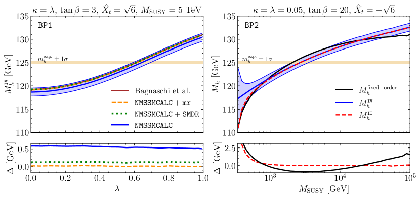
Figure 4: Left: Higgs mass prediction for the parameter point BP1 as a function of $\lambda$ using the quartic coupling matching. Shown are the results for $M_{h}^{\text{\tiny\Romanbar{4}}}$ and its uncertainty estimate defined in Eq. 3.63, obtained with NMSSMCALC (blue solid) or with a modified NMSSMCALC which uses mr (orange dashed) or SMDR (green dotted) for the SM OS-$\overline{\text{MS}}$ conversion and SM RGE-running. In brown we re-print the result taken from Fig.1 of Ref. [52]. The lower panel shows the differences of the result found in Ref. [52] and the results obtained with NMSSMCALC. Right: Higgs mass prediction for BP2 using the fixed-order (black), quartic coupling matching (blue), pole-mass matching (red dashed) calculation of NMSSMCALC. The blue band is the uncertainty of the quartic-coupling matching defined in Eq. 3.63. The lower panel shows the differences with the result obtained in the quartic-coupling matching.

Furthermore, the availability of the pole-mass matching also enables us to perform another cross-check. The pole-mass and quartic-coupling matching only differ by terms of $\order{\nicefrac{{v^{2}}}{{M_{\text{\tiny SUSY}}^{2}}}}$ and consequently should converge to each other for large $M_{\text{\tiny SUSY}}$ if all large logs appearing in the pole-mass calculation are cancelled properly. The two parameter points BP1 and BP2 are suitable for such a comparison as the BSM particle spectrum is of the order of the TeV-scale. In particular the stop masses, which control the numerically largest loop corrections, are above 2.5 TeV and hence the related uncertainties $\Delta^{\rm SUSY}_{v^{2}/M_{\text{\tiny SUSY}}^{2}}\sim\order{10\,\mathrm{MeV}}$ (cf. Table 4). This behaviour is demonstrated in Fig. 4 (right) for the parameter point BP2 where all SUSY particle masses are varied simultaneously with $M_{\text{\tiny SUSY}}$. The blue-solid line shows the Higgs mass prediction obtained using the quartic-coupling matching, $M_{h}^{\text{\tiny\Romanbar{4}}}$, while the red-dashed lines shows the result when using the pole-mass matching, $M_{h}^{\text{\tiny\Romanbar{2}}}$. In addition, we show the fixed-order result (black-solid) obtained in the $\overline{\text{DR}}$ scheme at $\order{\alpha_{t}(\alpha_{t}+\alpha_{s})}$. The lower panel in Fig. 4 (right) shows the difference $\Delta=M_{h}^{\text{\tiny\Romanbar{4}}}-M_{h}^{i}$ between the quartic coupling matching and the other two results. For large $M_{\text{\tiny SUSY}}$, starting from $M_{\text{\tiny SUSY}}>2\,\mathrm{TeV}$, we find perfect agreement between the pole-mass and quartic-coupling matching while for low $M_{\text{\tiny SUSY}}$ they can differ by several GeV. The blue uncertainty-band for $M_{h}^{\text{\tiny\Romanbar{4}}}$ also includes the differences to the pole-mass matching result, thereby demonstrating the importance of the $\nicefrac{{v^{2}}}{{M_{\text{\tiny SUSY}}^{2}}}$ corrections in this regime. On the other hand, the fixed-order result and the pole-mass matching show very good agreement for $M_{\text{\tiny SUSY}}\lesssim 1\,\mathrm{TeV}$ while for larger $M_{\text{\tiny SUSY}}$ the fixed-order line features a different shape and finally drops out of the uncertainty-band for $M_{\text{\tiny SUSY}}\gtrsim 50\,\mathrm{TeV}$. Therefore, the pole-mass matching procedure implemented in NMSSMCALC possesses features of a hybrid approach taking into account resummed logs as well as pieces of $\nicefrac{{v^{2}}}{{M_{\text{\tiny SUSY}}^{2}}}$ as the hybrid approaches in FlexibleEFTHiggs [48, 50, 49, 96] and FeynHiggs [3, 97, 98, 99, 100] do as it gives precise predictions for $M_{h}$ across a large range of $M_{\text{\tiny SUSY}}$ (see [7] for a complete list of references). However, parameter points like BP2 which are rather MSSM-like, often can only pass experimental constraints from stop searches, as well as the theoretical constraint of predicting $M_{h}\approx 125\,\mathrm{GeV}$, by having $M_{\text{\tiny SUSY}}$ larger than a few TeV and are therefore often saturated in the energy regime where a quartic coupling matching is sufficient. In the next section we show that this is not the case for the NMSSM, as it can predict a light singlet, which can greatly benefit from a pole-mass matching.

4.4 The Case of a Light Singlet

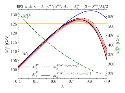
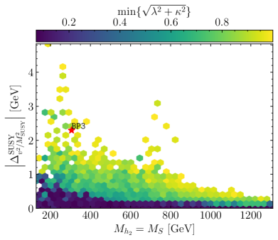
Figure 5: Left: The SM-like Higgs boson mass computed using the quartic-coupling matching (blue), pole-mass matching (red dashed), fixed-order $\order{\alpha_{t}(\alpha_{t}+\alpha_{s})}$ (black dashed) and the fixed-order $\order{\alpha_{t}\alpha_{s}+(\alpha_{t}+\alpha_{\lambda}+\alpha_{\kappa})^{2}}$ (black solid) calculation as a function of $\lambda$ for the parameter point BP3. The green line (to be read on the right axis), shows the mass-prediction of the singlet-like state obtained at fixed order $\order{\alpha_{t}\alpha_{s}+(\alpha_{t}+\alpha_{\lambda}+\alpha_{\kappa})^{2}}$. The red band is the uncertainty obtained for the pole-mass matching result, as defined in Eq. (3.62). Right: Size of the $v^{2}/M_{\text{\tiny SUSY}}^{2}$-type corrections as a function of the singlet mass for all parameter points obtained in the random scan. Each hexagonal bin shows the minimum value of $\sqrt{\lambda^{2}+\kappa^{2}}$ found in that bin.

We now consider the scenario of a rather light singlet which is realised by the parameter point BP3. In Fig. 5 (left) we show the Higgs boson mass prediction using the quartic-coupling matching (blue-solid), the pole-mass matching approach (red-dashed, including the red uncertainty band, applying Eq. (3.62)) and the fixed-order calculation at $\order{\alpha_{t}(\alpha_{t}+\alpha_{s})}$ (black dashed) and $\order{\alpha_{t}\alpha_{s}+(\alpha_{t}+\alpha_{\lambda}+\alpha_{\kappa})^{2}}$ (black solid) as a function of $\lambda$. The green line (to be read on the right axis) shows the fixed-order prediction for the mass $M_{S}$ of the singlet-like state. We scale the other NMSSM-parameters according to $\kappa=\lambda\cdot\kappa^{\texttt{\small BP3}}/\lambda^{\texttt{\small BP3}},\,A_{\kappa}=A_{\kappa}^{\texttt{\small BP3}}\cdot(3-\lambda^{\texttt{\small BP3}}/\lambda)/2$. This parametrisation allows us to vary $\lambda$ throughout a large range while maintaining a decreasing singlet mass with increasing $\lambda$ and it furthermore avoids the presence of tachyonic tree-level masses. For $\lambda=\lambda^{\texttt{\small BP3}}$ we recover the original parameter point. For small $\lambda\approx 0.4$ the singlet-like mass is about 500 GeV large while for large $\lambda\approx 0.9$ it can be as light as 250 GeV. The SM-like Higgs boson mass ranges between 100-131 GeV in the considered range. In the small-$\lambda$ (and large $M_{S}$) region we observe good agreement between all four methods. However, as $\lambda$ increases ($M_{S}$ decreases) the quartic-coupling matching result starts to deviate, reaching a difference w.r.t. the other results of up to $\sim 15\,\mathrm{GeV}$. It should be stressed that the stop masses are always above 1.5 TeV for this parameter point. Therefore, all $\nicefrac{{v^{2}}}{{M_{\text{\tiny SUSY}}^{2}}}$ contributions from the stop sector are negligible compared to those originating in the singlet sector.

It remains the question whether missing higher-order corrections to the matching condition proportional to $\lambda$ and $\kappa$ can become significant for large $\lambda$. The leading two-loop corrections of this type to the matching condition have been computed in Ref. [52] and are currently not available in NMSSMCALC. We therefore estimate the importance of NMSSM-specific corrections by comparing with the two-loop fixed-order prediction that implements these corrections [32]. In Fig. 5 (left) we observe, that the relative size of the NMSSM-specific higher-order corrections in the fixed-order calculation is always much smaller than the relative size of the missing $\nicefrac{{v^{2}}}{{M_{\text{\tiny SUSY}}^{2}}}$ contributions in the EFT-approach. Therefore, the $\nicefrac{{v^{2}}}{{M_{\text{\tiny SUSY}}^{2}}}$ corrections in the one-loop matching condition of the quartic-coupling approach are numerically more significant than the missing NMSSM-specific higher-order corrections to the matching condition. Regarding the pole-mass matching the evaluation of the importance of the missing two-loop corrections is left for future work.

The region in Fig. 5 (left) that features very large $\Delta^{\rm SUSY}_{v^{2}/M_{\text{\tiny SUSY}}^{2}}$ is clearly not in agreement with the Higgs boson mass measurement. In Fig. 5 (right) we study the size of the $\nicefrac{{v^{2}}}{{M_{\text{\tiny SUSY}}^{2}}}$ terms by plotting the absolute value of $\Delta^{\rm SUSY}_{v^{2}/M_{\text{\tiny SUSY}}^{2}}$ for all parameter points found in the random scan, which fulfill all applied constraints and feature a second-lightest singlet-like scalar, as a function of the singlet mass $M_{S}$. The parameter points are grouped in hexagonal bins whereas the color of each bin indicates the minimum value of $\sqrt{\lambda^{2}+\kappa^{2}}$ found in that bin. We observe that $\Delta^{\rm SUSY}_{v^{2}/M_{\text{\tiny SUSY}}^{2}}$ tends to decrease for increasing $M_{S}$ and therefore shows a similar behaviour as the stop sector (note that e.g. the neutralinos could still be lighter than the singlet and also cause $\nicefrac{{v^{2}}}{{M_{\text{\tiny SUSY}}^{2}}}$ contributions). However, the size of $\Delta^{\rm SUSY}_{v^{2}/M_{\text{\tiny SUSY}}^{2}}$ is also strongly influenced by the size of $\lambda$ and $\kappa$. For $\sqrt{\lambda^{2}+\kappa^{2}}\lesssim 0.2$ we find $\Delta^{\rm SUSY}_{v^{2}/M_{\text{\tiny SUSY}}^{2}}\lesssim 1\,\mathrm{GeV}$ which is similar to what we obtain in the MSSM with the present exclusion limits on the stops. It is remarkable that the two matching approaches agree with each other reasonably well for small $\lambda$ and $\kappa$ even if the singlet is as light as 200 GeV (cf. dark blue points in the plot). However, for $\sqrt{\lambda^{2}+\kappa^{2}}\gtrsim 0.3$ the quartic-coupling matching would suffer from large missing $\nicefrac{{v^{2}}}{{M_{\text{\tiny SUSY}}^{2}}}$ corrections, which can reach up to $\order{5\,\mathrm{GeV}}$ for $\sqrt{\lambda^{2}+\kappa^{2}}\gtrsim 0.9$.

4.5 CP-Violating Effects in the EFT Calculations

In the following we study the effect of non-vanishing CP-violating phases onto the Higgs mass prediction at the example of the parameter points BP1 and BP3. We distinguish two scenarios: (i) CP in the Higgs sector is conserved at the tree-level but broken by loop effects from the SUSY fermions and scalars and (ii) CP is already broken at the tree-level.

4.5.1 Loop-induced CP-Violation

In Fig. 6 we show the Higgs mass prediction for BP1 (left) and BP3 (right) for individually varied phases of $M_{1}$ (blue), $M_{2}$ (black) and $A_{t}$ (red). The lower panels show the prediction for the electric dipole moment of the electron (eEDM) obtained with NMSSMCALC normalised to the current experimental upper bound [101]. The solid lines show the Higgs mass prediction obtained with the pole-mass matching while the dashed lines are obtained with the quartic-coupling matching. In addition, the results of the quartic-coupling matching have been shifted by the constant difference $\left.\Delta^{\rm SUSY}_{v^{2}/M_{\text{\tiny SUSY}}^{2}}\right|_{\varphi_{i}=0}$ from Table 4 such that the dashed and solid lines overlap for $\varphi=0$. Therefore, one can directly read-off additional $\nicefrac{{v^{2}}}{{M_{\text{\tiny SUSY}}^{2}}}$-effects caused by the CP-violating phases. For both parameter points we find that $\varphi_{A_{t}}$ is not constrained by the eEDM while still having an effect on $M_{h}$ of $\order{1\,\mathrm{GeV}}$. The phases $\varphi_{M_{1,2}}$ can have a similar effect on $M_{h}$ but are strongly constrained when varied individually. It should be noted, however, that for some choices of $\varphi_{M_{1}}\neq\varphi_{M_{2}}\neq 0$ the EDM constraints can be avoided while still achieving non-negligible effects on $M_{h}$.

The $\nicefrac{{v^{2}}}{{M_{\text{\tiny SUSY}}^{2}}}$ effects caused by the CP-violating phases are negligible for the parameter point BP1 since all SUSY particles are heavy in this scenario. This is not the case for BP3, which has a rather light neutralino and therefore a large $\left.\Delta^{\rm SUSY}_{v^{2}/M_{\text{\tiny SUSY}}^{2}}\right|_{\varphi_{M_{2}}\neq 0}$ contribution.

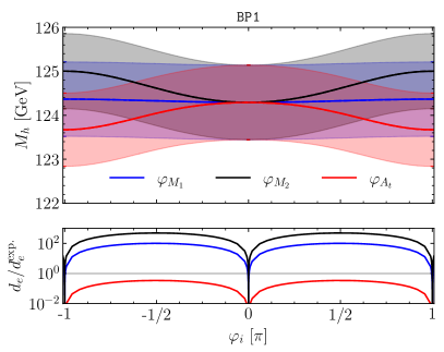
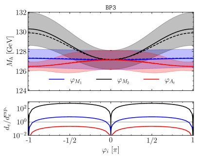
Figure 6: The dependence of the Higgs mass prediction using the pole-mass matching (solid) and quartic-coupling matching (dashed) on the CP-violating phases of $M_{1}$ (blue), $M_{2}$ (black) and $A_{t}$ (red). The quartic-coupling matching results have been shifted by the constant values $\left.\Delta^{\rm SUSY}_{v^{2}/M_{\text{\tiny SUSY}}^{2}}\right|_{\varphi_{i}=0}$ from Table 4.

4.5.2 Tree-level CP-Violation

Considering Eq. 3.29c any phase-combination $\varphi_{y}=2\varphi_{s}+\varphi_{\kappa}-\varphi_{\lambda}-\varphi_{u}\neq 0$ will immediately introduce CP-violating effects in the Higgs sector thereby having a strong impact on the EDM prediction. In the following we focus on $\varphi_{\lambda}$ and $\varphi_{\kappa}$ which were found to have the smallest impact on the eEDM for the considered parameter points.

In Fig. 7 we show the same quantities as in Fig. 6 but as a function of $\varphi_{\kappa}$ (red) and $\varphi_{\lambda}$ (blue). We find that for BP1 $|\varphi_{\lambda}|\gtrsim 0.05$ ($|\varphi_{\kappa}|\gtrsim 0.15$) and for BP3 $|\varphi_{\lambda}|\gtrsim 0.01$ ($|\varphi_{\kappa}|\gtrsim 0.03$) is excluded by the eEDM. However, even in these small ranges the Higgs mass prediction depends strongly on the CP-violating phases. Concerning the size of the $\nicefrac{{v^{2}}}{{M_{\text{\tiny SUSY}}^{2}}}$ contributions, the picture is similar to the loop-induced CP-case i.e. only BP3 shows a significant difference between pole-mass and quartic-coupling matching.

As an additional cross-check we verified that pole-mass and quartic-coupling matching (i.e. solid and dashed lines of the same color) are in agreement for all values considered in Figs. 6 and 7 once we set the running VEV $v(Q_{\text{match}})$ at the matching scale to a numerically small value in the pole-mass matching which effectively turns-off all $\nicefrac{{v^{2}}}{{M_{\text{\tiny SUSY}}^{2}}}$ corrections. However, for very large values of $|\lambda|,\,|\kappa|$ and $\varphi_{y}\sim\order{1}$ one may induce sizeable mixing between CP-even and CP-odd Higgs fields (such that the SM is no longer the right EFT) even for $v\to 0$. Thus, CP-violating cases with very large CP-even/odd mixing have to be considered with caution. The matching to appropriate EFTs that are not the SM but include more light degrees of freedom is left for future work.

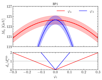
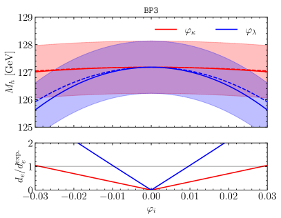
Figure 7: The dependence of the Higgs mass prediction using the pole-mass matching (solid) and quartic-coupling matching (dashed) on the CP-violating phases of $\lambda$ (blue) and $\kappa$ (red). The quartic-coupling matching results have been shifted by the constant values $\left.\Delta^{\rm SUSY}_{v^{2}/M_{\text{\tiny SUSY}}^{2}}\right|_{\varphi_{i}=0}$ from Table 4.

5 Conclusions

In this paper, we presented our new computation of the higher-order corrections to the SM-like Higgs boson of the CP-violating NSSM for large mass hierarchies. In this case, fixed-order computations become unreliable due to the involved logarithms of large mass hierarchies, requiring the application of an EFT framework. We chose a scenario where all non-SM particles are very heavy, so that the low-energy EFT is given by the SM. The matching of the full NMSSM to the SM at the high-scale is performed at full one-loop order in the NMSSM, including two-loop corrections in the MSSM limit. We applied two matching approaches given by the quartic coupling matching in the unbroken theory and the pole mass matching after EWSB. The latter includes terms of the order $v^{2}/M_{\text{\tiny SUSY}}^{2}$, so that the comparison between the two methods allowed us to estimate the importance of these terms that are neglected in the former approach. We additionally provided an estimate of the different sources of uncertainty. Our new computation has been implemented in the public program package NMSSMCALC and can be downloaded from the url:

https://www.itp.kit.edu/~maggie/NMSSMCALC/

For our numerical analysis, we performed a scan in the NMSSM parameter space and only kept points that are in agreement with the Higgs signal data and exclusion constraints on additional Higgs bosons and supersymmetric particles. We validated our calculation and implementation of the two matching procedures in NMSSMCALC against existing results in the literature and found good agreement for the tested parameter point. We subsequently investigated the case of a light singlet-like Higgs boson in the NMSSM spectrum. As expected, the EFT approach applying the pole-mass matching shows good agreement with the fixed-order result (including partly resummation in the top/stop sector by applying $\overline{\text{DR}}$ renormalisation [31]) within the theoretical uncertainty, while the quartic coupling matching starts more and more deviating with decreasing singlet mass due to the missing ${\cal O}(v^{2}/M_{\text{\tiny SUSY}}^{2})$ terms. The behavior is confirmed by the analysis of our entire found parameter sample. With increasing values of the specific NMSSM coupling parameters $\lambda$ and $\kappa$, the singlet-like Higgs boson mass decreases, and the $v^{2}/M_{\text{\tiny SUSY}}^{2}$ effects beome increasingly important, deteriorating the description by the quartic coupling matching. Within the uncertainty band of the pole-mass matching, the two matching approached nevertheless can agree with each other even if the singlet mass is as light as 200 GeV provided that $\sqrt{\lambda^{2}+\kappa^{2}}\lesssim 0.2$. We studied, for the first time the effects of CP violation in the EFT approach in the NMSSM. From a conceptional point of view, we found that care has to be taken in the derivation of the quartic-coupling matching not to miss finite contributions that do not appear in the CP-conserving case nor the CP-violating MSSM. This requires the expansion of the tadpoles up to ${\cal O}(v\times M_{\text{\tiny SUSY}}^{2})$. Both for loop-induced and tree-level CP violation, we find the $v^{2}/M_{\text{\tiny SUSY}}^{2}$ contributions to the matching condition to become important for our benchmark point BP3 which features a light singlet Higgs boson.

In summary, our EFT implementation based on the pole-mass and the quartic-coupling matching is in good agreement within theoretical uncertainties and reliably describes NMSSM scenarios with a heavy non-SM mass spectrum. Scenarios with light singlet-like states (i.e. lighter than 125 GeV) require the extension of the approach beyond the SM as effective low-enery description. This is left for future work.

Appendix A Expansion of the One-Loop Tadpoles to $\mathcal{O}(v)$

In this appendix we derive the leading terms of $\delta^{(1)}t_{a_{d}}/v$ which are not suppressed by inverse powers of $M_{\text{\tiny SUSY}}$. The tadpole counterterm $\delta^{(1)}t_{a_{d}}$ can be expanded to $\order{v\times M_{\text{\tiny SUSY}}^{2}}$ in two equivalent ways. The first method involves considerations about the dependence of couplings, mixing matrices and mass eigenvalues on the SM VEV. The second method relies on a systematic expansion in $v$.

Method (i):

The couplings entering the Feynman diagrams of $\delta^{(1)}t_{a_{d}}$ in general consist of a linear combination of $v$-independent factors, which correspond to couplings defined in the gauge-basis (or unbroken EW phase) and of $v$-dependent mixing-matrices. The lowest dependence of the mass eigenvalues on $v$ is of ${\cal O}(v^{2})$ in the tadpole diagrams. The only linear dependence on $v$ arises in the mixing matrices that hence need to be expanded to $\order{v}$. The expansion of the mixing matrices can be performed by using the solutions of the rotation matrices that have been obtained analytically for the case $v=0$ as an ansatz and introducing $\order{v}$-terms on the off-diagonal elements. These elements can be determined by requiring unitarity of the mixing matrix up to $\order{v^{2}/M_{\text{\tiny SUSY}}^{2}}$ and by requiring that the mass matrix with the full $v$-dependence is diagonalised up to $\order{v^{2}/M_{\text{\tiny SUSY}}^{2}}$. For the example of the stop-mixing matrix $\tilde{U}$ we find at $\order{v/M_{\text{\tiny SUSY}}}$:

$$\tilde{U}_{ii} =1,\,$$

$$\tilde{U}_{12} =-\left(\tilde{U}_{21}\right)^{*}=\frac{v}{2}\frac{\sqrt{2}e^{i(\varphi_{w}-\varphi_{y}+\varphi_{A_{t}})}|A_{t}|-|\lambda|v_{s}\cot\beta}{m_{\tilde{Q}_{3}}^{2}-m_{\tilde{U}_{R,3}}^{2}}e^{\varphi_{\lambda}+\varphi_{s}}\,,$$

whereas the squared mass-eigenvalues do not receive additional corrections at $\order{v^{2}/M_{\text{\tiny SUSY}}^{2}}$ but only at $\order{v^{2}/M_{\text{\tiny SUSY}}^{2}}$. The resulting stop-contribution to the counterterm reads

$$\delta^{(1)}t_{a_{d}}=v\frac{3|\lambda||A_{t}|v_{s}Y_{t}^{2}}{16\pi^{2}\sqrt{2}\sin\beta}B(m_{\tilde{Q}_{3}},m_{\tilde{U}_{R,3}})\sin(\varphi_{w}-\varphi_{y}+\varphi_{A_{t}})\,,$$ (A.72)

with

$$B(x,y) =\frac{A(x)-A(y)}{x^{2}-y^{2}}\,,$$

$$B(x,x) =\ln\frac{\mu^{2}}{x^{2}}\,,$$

$$A(x) =x^{2}\left(1+\ln\frac{\mu^{2}}{x^{2}}\right)\,,$$

$$A(0) =0\,.$$

Method (ii):

A systematic way of computing the tadpole without performing an explicit expansion of mixing matrix elements can be performed by considering the Taylor expansion of the tadpole counter-term around $v=0$:

$$\delta^{(1)}t_{a_{d}}=v\cdot\left.\frac{\partial t_{a_{d}}}{\partial v}\right|_{v=0}+\order{v^{2}}\,.$$ (A.73)

The tadpole itself can be written as the derivative of the one-loop effective potential $V^{(1)}$ w.r.t. the field $a_{d}$, i.e. $\delta^{(1)}t_{a_{d}}=\partial V^{(1)}/\partial a_{d}$. The derivative of the potential w.r.t. the SM-like Higgs VEV $v$ can be replaced by the derivative w.r.t. the Higgs field itself. Thus, we find

$$\delta^{(1)}t_{a_{d}} =v\cdot\left.\frac{\partial^{2}V(h,a_{d},\dots)}{\partial a_{d}\partial h}\right|_{h=a_{d}=0;v=0}+\order{v^{2}}$$ (A.74a)

$$=v\cdot\left.\Sigma_{h\to a_{d}}(p^{2}=0)\right|_{v=0}+\order{v^{2}}$$ (A.74b)

$$=v\cdot\left.\left(\sin\beta\Sigma_{h\to G}(p^{2}=0)-\cos\beta\Sigma_{h\to A}(p^{2}=0)\right)\right|_{v=0}+\order{v^{2}}\,,$$ (A.74c)

where in the second line we used that the second derivative of the effective potential is equivalent to the self-energy evaluated at vanishing external momentum. In the last line we rotated the second index of the $i\to j$ self-energy from the gauge-basis into the mass-basis using Eq. 2.10. Note that the self-energy is again computed in the unbroken phase and can be conveniently generated with e.g. SARAH. Using this result we find full agreement with the stop contribution derived above. Furthermore, we also compute the full result including contributions from electroweakinos as well as the neutral and charged Higgses and found full agreement (within the numerical accuracy) with the result obtained when evaluating $\delta^{(1)}t_{a_{d}}/v$ numerically for $v=1\,\mathrm{GeV}$.

Appendix B New Implementation in NMSSMCALC

In this appendix we describe how the new and old Higgs mass prediction in NMSSMCALC is controlled using the SLHA interface, and discuss examples of in- and output files.

The SLHA NMSSM input parameters are interpreted as $\overline{\text{DR}}$ parameters at the scale $Q_{\rm inp.}$ (cf. Fig. 1 box 1b)). The fixed-order calculation implemented in NMSSMCALC allows to renormalise the charged Higgs boson mass $M_{H^{\pm}}^{\rm OS}$ on-shell or to alternatively compute the charged Higgs boson mass at two-loop order and use $\text{Re}A_{\lambda}^{\overline{\text{DR}}}$ as input. Furthermore, NMSSMCALC has two options for the renormalisation scheme for the top/stop sector: on-shell and $\overline{\text{DR}}$. In contrast, the newly implemented EFT calculation currently only takes SUSY contributions in the $\overline{\text{DR}}$ scheme into account. Thus, we recommend to use the $\overline{\text{DR}}$ scheme in combination with the EFT calculation. However, it is in principle still possible to choose a different (the OS) scheme in the precision fixed-order prediction of the BSM masses by using the flags 7 and 8 in the MODSEL block, cf. Fig. 8. With flag 6, the user chooses the loop-order of the fixed-order calculation. These flags only concern the fixed-order calculations which are written out into the MASS block. In addition, there are three new flags, 15, 16 and 17, to control the calculation of the SM-like Higgs boson mass. If the EFT calculation was chosen by setting the flag 15 to a value larger than 10, the entry of the SM-like Higgs boson mass is overwritten with the EFT result while all other MASS entries are those obtained with the fixed-order calculation (flags 6,7,8). For scenarios, where the SM-like Higgs is the lightest of the neutral Higgs bosons, this would be the entry of “MASS 25”. If, however, the dominantly $h_{u}$-like Higgs boson is not the lightest neutral Higgs boson, the entry of the heavier neutral Higgs state corresponding to the SM-like Higgs is overwritten with the EFT result. In this case, however, the EFT approach is not valid any more as it assumes all other Higgs bosons to be heavy. The NMHMIXC block, containing the numerical values of the neutral Higgs mixing matrix, corresponds to the matrix that diagonalises the loop-corrected mass matrix if the fixed-order calculation was was chosen by the user. If the EFT calculation is chosen, NMHMIXC corresponds to the tree-level mixing matrix. Setting flag 15 to -2, the program decides whether the fixed-order or the EFT calculation is performed, for scenarios where the size of the SUSY input scale (given in “EXTPAR 0”) is larger than 1.5 TeV. The input scale, if not specified by the user, by default is set to $Q_{\text{inp}}=\sqrt{m_{\tilde{Q}_{3}}m_{\tilde{u}_{R_{3}}}}$, which indicates the size of the stop masses. Scenarios with e.g. a light singlet, where the EFT approach might be questionable, are therefore not recognised by this estimate. If flag 15 is set to -1, the program always uses the fixed-order rather than the EFT calculation. For flag 15 being between 11 and 24, the first digit (1 or 2) determines the EFT approach (pole-mass or quartic-coupling matching) and the second digit turns on various higher-order corrections in the EFT calculation, cf. Fig. 8. These are the full NMSSM one-loop corrections including CP-violating effects computed in this work and the 2-loop corrections in the MSSM limit at ${\cal O}(\alpha_{s}\alpha_{t})$ [67], ${\cal O}(\alpha_{t}^{2})$ [67], and ${\cal O}(\alpha_{s}\alpha_{\text{EW}})$ [68]. Setting flag 16 to 12 or 22 chooses the $\alpha_{M_{Z}}$ or the $G_{F}$-scheme in the extraction of the SM $\overline{\text{MS}}$ parameters while flag 17 controls the uncertainty estimate of the EFT calculation. In Fig. 9 we show the new DMASS block, which contains the theoretical uncertainty of the EFT result, obtained for the parameter point BP3 with the settings given in Fig. 8. In addition to the total uncertainty (“DMASS 25”, corresponding to Eq. 3.62), it also lists the individual uncertainties as well as the difference to the fixed-order result obtained with the MODSEL flags 6, 7 and 8. The mass uncertainty of the BSM Higgs masses is set to the commonly chosen fixed value of 3 GeV. This is often larger than the overall size of the loop-corrections to the scalar BSM masses and therefore a rather conservative estimate.

Block MODSEL
_3__1__# NMSSM
_5__2__# 0:CP-conserving; 2:general CP-violation
_6__3__# loop level of fixed-order calculations:
_______#__1:one-loop; 2:$\order{\alpha_{t}\alpha_{s}}$; 3:$\order{\alpha_{t}\alpha_{s}+\alpha_{t}^{2}}$;
_______#__4:$\order{\alpha_{t}\alpha_{s}+(\alpha_{t}+\alpha_{\lambda}+\alpha_{\kappa})^{2}}$
_7__2__# top/stop sector (in fixed-order calculation):
_______#__2:$\overline{\text{DR}}$; 3:OS scheme
_8__0__# 0:MHpm as OS-input; 1:ReAlambda as $\overline{\text{DR}}$-input
_10 0__# EDM calculation:0/1/2 (off/on/detailed output)
_11 0__# AMMM calculation:0/1/2 (off/on/detailed output)
_12 0__# compute effective HHH couplings:0/1 (off/on)
_13 0__# loop-corrected W-mass:0/1 (off/on)
_15 14 # fixed-order or EFT.
_______#__-2:automatic; -1:always fixed-order;
_______#__1n/2n:EFT with pole-mass/quartic matching
_______#________at n-order with n=1:one-loop (this work);
_______#_______ n=2:$\order{\alpha_{s}\alpha_{t}}$ [67]; n=3:$\order{\alpha_{t}^{2}}$ [67];
_______#_______ n=4:$\order{\alpha_{s}\alpha_{\text{EW}}}$ [68]
_16 22 # extraction of $\overline{\text{MS}}$ SM parameters using
_______#__$\alpha_{M_{Z}}$-scheme (12) or $G_{F}$-scheme (22)
_17 1__# uncertainty estimate:0/1 (off/on)

Figure 8: Example of all new and old flags available in the MOSDEL-block of the SLHA input-file.

BLOCK DMASS # Theoreticalerror
__25__9.52016291E-01 # H1
__35__3.00000000E+00 # H2
__36__3.00000000E+00 # H3
__45__3.00000000E+00 # H4
__46__3.00000000E+00 # H5
__37__3.00000000E+00 # Hc
_251_-8.17298889E-01 # $M_{h}({Q_{\text{match}}=Q_{\text{inp}}})-M_{h}({Q_{\text{match}}=Q_{\text{inp}}/2})$
_252__8.38518143E-01 # $M_{h}({Q_{\text{match}}=Q_{\text{inp}}})-M_{h}({Q_{\text{match}}=2Q_{\text{inp}}})$
_253_-4.01258469E-01 # $\Delta^{{\text{SM}}}_{Y_{t}}=M_{h}(Y_{t}^{{{\text{SM}}},\order{\alpha_{s}^{3}}})-M_{h}(Y_{t}^{{{\text{SM}}},\order{\alpha_{s}^{2}}})$
_254__2.09808350E-02 # $\Delta^{{\text{SM}}}_{G_{F}/\alpha_{M_{Z}}}=M_{h}^{G_{F}}-M_{h}^{\alpha_{M_{Z}}}$
_255_-2.29334831E+00 # estimated size of $\nicefrac{{v^{2}}}{{M_{\text{\tiny SUSY}}^{2}}}$ terms ($\Delta_{v^{2}/M_{\text{\tiny SUSY}}^{2}}^{\mathrm{SUSY}}$)
_256_-7.32089989E-02 # ${M_{h}^{\texttt{EFT}}-M_{h}^{\texttt{fixed-order}}}$ (not included in total uncertainty)
_257__2.04386369E-01 # SM scale uncertainty ($\Delta^{{\text{SM}}}_{Q_{\text{EW}}}$)

Figure 9: Example of the DMASS block in the SLHA output-file. The numerical values correspond to the output obtained for the benchmark point BP3 using the pole-mass matching (MODSEL 15=14) and the $G_{F}$-scheme (MODSEL 16=22).

References

- [1] ATLAS Collaboration collaboration, Observation of a new particle in the search for the Standard Model Higgs boson with the ATLAS detector at the LHC, Phys.Lett. B716 (2012) 1 [1207.7214].
- [2] CMS Collaboration collaboration, Observation of a new boson at a mass of 125 GeV with the CMS experiment at the LHC, Phys.Lett. B716 (2012) 30 [1207.7235].
- [3] T. Hahn, S. Heinemeyer, W. Hollik, H. Rzehak and G. Weiglein, High-Precision Predictions for the Light CP -Even Higgs Boson Mass of the Minimal Supersymmetric Standard Model, Phys. Rev. Lett. 112 (2014) 141801 [1312.4937].
- [4] J.R. Ellis, J. Gunion, H.E. Haber, L. Roszkowski and F. Zwirner, Higgs Bosons in a Nonminimal Supersymmetric Model, Phys.Rev. D39 (1989) 844.
- [5] M. Drees, Supersymmetric Models with Extended Higgs Sector, Int.J.Mod.Phys. A4 (1989) 3635.
- [6] M. Maniatis, The Next-to-Minimal Supersymmetric extension of the Standard Model reviewed, Int.J.Mod.Phys. A25 (2010) 3505 [0906.0777].
- [7] P. Slavich et al., Higgs-mass predictions in the MSSM and beyond, Eur. Phys. J. C 81 (2021) 450 [2012.15629].
- [8] U. Ellwanger, Radiative corrections to the neutral Higgs spectrum in supersymmetry with a gauge singlet, Phys. Lett. B 303 (1993) 271 [hep-ph/9302224].
- [9] T. Elliott, S. King and P. White, Supersymmetric Higgs bosons at the limit, Phys.Lett. B305 (1993) 71 [hep-ph/9302202].
- [10] T. Elliott, S. King and P. White, Squark contributions to Higgs boson masses in the next-to-minimal supersymmetric standard model, Phys.Lett. B314 (1993) 56 [hep-ph/9305282].
- [11] T. Elliott, S. King and P. White, Radiative corrections to Higgs boson masses in the next-to-minimal supersymmetric Standard Model, Phys.Rev. D49 (1994) 2435 [hep-ph/9308309].
- [12] P. Pandita, One loop radiative corrections to the lightest Higgs scalar mass in nonminimal supersymmetric Standard Model, Phys. Lett. B 318 (1993) 338.
- [13] P. Pandita, Radiative corrections to the scalar Higgs masses in a nonminimal supersymmetric Standard Model, Z. Phys. C 59 (1993) 575.
- [14] S. King and P. White, Resolving the constrained minimal and next-to-minimal supersymmetric standard models, Phys. Rev. D 52 (1995) 4183 [hep-ph/9505326].
- [15] U. Ellwanger and C. Hugonie, Yukawa induced radiative corrections to the lightest Higgs boson mass in the NMSSM, Phys. Lett. B 623 (2005) 93 [hep-ph/0504269].
- [16] G. Degrassi and P. Slavich, On the radiative corrections to the neutral Higgs boson masses in the NMSSM, Nucl. Phys. B 825 (2010) 119 [0907.4682].
- [17] F. Staub, W. Porod and B. Herrmann, The Electroweak sector of the NMSSM at the one-loop level, JHEP 1010 (2010) 040.
- [18] P. Drechsel, L. Galeta, S. Heinemeyer and G. Weiglein, Precise Predictions for the Higgs-Boson Masses in the NMSSM, Eur. Phys. J. C 77 (2017) 42.
- [19] S. Ham, J. Kim, S. Oh and D. Son, The Charged Higgs boson in the next-to-minimal supersymmetric standard model with explicit CP violation, Phys.Rev. D64 (2001) 035007 [hep-ph/0104144].
- [20] S. Ham, S. Oh and D. Son, Neutral Higgs sector of the next-to-minimal supersymmetric standard model with explicit CP violation, Phys. Rev. D 65 (2002) 075004 [hep-ph/0110052].
- [21] S. Ham, Y. Jeong and S. Oh, Radiative CP violation in the Higgs sector of the next-to-minimal supersymmetric model, hep-ph/0308264.
- [22] K. Funakubo and S. Tao, The Higgs sector in the next-to-MSSM, Prog.Theor.Phys. 113 (2005) 821 [hep-ph/0409294].
- [23] S. Ham, S. Kim, S. Oh and D. Son, Higgs bosons of the NMSSM with explicit CP violation at the ILC, Phys.Rev. D76 (2007) 115013 [0708.2755].
- [24] K. Cheung, T.-J. Hou, J.S. Lee and E. Senaha, The Higgs Boson Sector of the Next-to-MSSM with CP Violation, Phys.Rev. D82 (2010) 075007 [1006.1458].
- [25] M.D. Goodsell and F. Staub, The Higgs mass in the CP violating MSSM, NMSSM, and beyond, Eur. Phys. J. C 77 (2017) 46.
- [26] F. Domingo, P. Drechsel and S. Paßehr, On-Shell neutral Higgs bosons in the NMSSM with complex parameters, Eur. Phys. J. C77 (2017) 562 [1706.00437].
- [27] M.D. Goodsell, K. Nickel and F. Staub, Two-loop corrections to the Higgs masses in the NMSSM, Phys. Rev. D91 (2015) 035021.
- [28] K. Ender, T. Graf, M. Muhlleitner and H. Rzehak, Analysis of the NMSSM Higgs Boson Masses at One-Loop Level, Phys. Rev. D 85 (2012) 075024.
- [29] T. Graf, R. Grober, M. Muhlleitner, H. Rzehak and K. Walz, Higgs Boson Masses in the Complex NMSSM at One-Loop Level, JHEP 10 (2012) 122.
- [30] M. Mühlleitner, D.T. Nhung, H. Rzehak and K. Walz, Two-loop contributions of the order to the masses of the Higgs bosons in the CP-violating NMSSM, JHEP 05 (2015) 128 [1412.0918].
- [31] T.N. Dao, R. Gröber, M. Krause, M. Mühlleitner and H. Rzehak, Two-loop ( ) corrections to the neutral Higgs boson masses in the CP-violating NMSSM, JHEP 08 (2019) 114 [1903.11358].
- [32] T.N. Dao, M. Gabelmann, M. Mühlleitner and H. Rzehak, Two-loop ((t + λ + κ)2) corrections to the Higgs boson masses in the CP-violating NMSSM, JHEP 09 (2021) 193 [2106.06990].
- [33] J. Baglio, R. Grober, M. Muhlleitner, D. Nhung, H. Rzehak et al., NMSSMCALC: A Program Package for the Calculation of Loop-Corrected Higgs Boson Masses and Decay Widths in the (Complex) NMSSM, Comput.Phys.Commun. 185 (2014) 3372 [1312.4788].
- [34] D.T. Nhung, M. Muhlleitner, J. Streicher and K. Walz, Higher Order Corrections to the Trilinear Higgs Self-Couplings in the Real NMSSM, JHEP 1311 (2013) 181 [1306.3926].
- [35] M. Mühlleitner, D.T. Nhung and H. Ziesche, The order corrections to the trilinear Higgs self-couplings in the complex NMSSM, JHEP 12 (2015) 034.
- [36] C. Borschensky, T.N. Dao, M. Gabelmann, M. Mühlleitner and H. Rzehak, The trilinear Higgs self-couplings at in the CP-violating NMSSM, Eur. Phys. J. C 83 (2023) 118 [2210.02104].
- [37] T.N. Dao, M. Gabelmann and M. Mühlleitner, The correction to the parameter and its effect on the W boson mass calculation in the complex NMSSM, Eur. Phys. J. C 83 (2023) 1079 [2308.04059].
- [38] U. Ellwanger, J.F. Gunion and C. Hugonie, NMHDECAY: A Fortran code for the Higgs masses, couplings and decay widths in the NMSSM, JHEP 02 (2005) 066 [hep-ph/0406215].
- [39] U. Ellwanger and C. Hugonie, NMHDECAY 2.0: An Updated program for sparticle masses, Higgs masses, couplings and decay widths in the NMSSM, Comput. Phys. Commun. 175 (2006) 290 [hep-ph/0508022].
- [40] F. Staub, From Superpotential to Model Files for FeynArts and CalcHep/CompHep, Comput.Phys.Commun. 181 (2010) 1077 [0909.2863].
- [41] F. Staub, Automatic Calculation of supersymmetric Renormalization Group Equations and Self Energies, Comput.Phys.Commun. 182 (2011) 808 [1002.0840].
- [42] F. Staub, SARAH 3.2: Dirac Gauginos, UFO output, and more, Computer Physics Communications 184 (2013) pp. 1792 [1207.0906].
- [43] F. Staub, SARAH 4: A tool for (not only SUSY) model builders, Comput.Phys.Commun. 185 (2014) 1773 [1309.7223].
- [44] W. Porod, SPheno, a program for calculating supersymmetric spectra, SUSY particle decays and SUSY particle production at e+ e- colliders, Comput. Phys. Commun. 153 (2003) 275 [hep-ph/0301101].
- [45] W. Porod and F. Staub, SPheno 3.1: Extensions including flavour, CP-phases and models beyond the MSSM, Comput. Phys. Commun. 183 (2012) 2458 [1104.1573].
- [46] B.C. Allanach, SOFTSUSY: a program for calculating supersymmetric spectra, Comput. Phys. Commun. 143 (2002) 305 [hep-ph/0104145].
- [47] B.C. Allanach and T. Cridge, The Calculation of Sparticle and Higgs Decays in the Minimal and Next-to-Minimal Supersymmetric Standard Models: SOFTSUSY4.0, Comput. Phys. Commun. 220 (2017) 417 [1703.09717].
- [48] P. Athron, J.-h. Park, D. Stöckinger and A. Voigt, FlexibleSUSY—A spectrum generator generator for supersymmetric models, Comput. Phys. Commun. 190 (2015) 139 [1406.2319].
- [49] P. Athron, M. Bach, D. Harries, T. Kwasnitza, J.-h. Park, D. Stöckinger et al., FlexibleSUSY 2.0: Extensions to investigate the phenomenology of SUSY and non-SUSY models, Comput. Phys. Commun. 230 (2018) 145 [1710.03760].
- [50] P. Athron, J.-h. Park, T. Steudtner, D. Stöckinger and A. Voigt, Precise Higgs mass calculations in (non-)minimal supersymmetry at both high and low scales, JHEP 01 (2017) 079 [1609.00371].
- [51] F. Staub and W. Porod, Improved predictions for intermediate and heavy Supersymmetry in the MSSM and beyond, Eur. Phys. J. C 77 (2017) 338 [1703.03267].
- [52] E. Bagnaschi, M. Goodsell and P. Slavich, Higgs-mass prediction in the NMSSM with heavy BSM particles, Eur. Phys. J. C 82 (2022) 853 [2206.04618].
- [53] J. Baglio, T.N. Dao and M. Mühlleitner, One-Loop Corrections to the Two-Body Decays of the Neutral Higgs Bosons in the Complex NMSSM, Eur. Phys. J. C 80 (2020) 960 [1907.12060].
- [54] H. Bahl and I. Sobolev, Two-loop matching of renormalizable operators: general considerations and applications, JHEP 03 (2021) 286 [2010.01989].
- [55] D. Buttazzo, G. Degrassi, P.P. Giardino, G.F. Giudice, F. Sala, A. Salvio et al., Investigating the near-criticality of the Higgs boson, JHEP 12 (2013) 089 [1307.3536].
- [56] I. Schienbein, F. Staub, T. Steudtner and K. Svirina, Revisiting RGEs for general gauge theories, Nucl. Phys. B 939 (2019) 1 [1809.06797].
- [57] K.G. Chetyrkin and M.F. Zoller, Three-loop \beta-functions for top-Yukawa and the Higgs self-interaction in the Standard Model, JHEP 06 (2012) 033 [1205.2892].
- [58] K.G. Chetyrkin and M.F. Zoller, Leading QCD-induced four-loop contributions to the -function of the Higgs self-coupling in the SM and vacuum stability, JHEP 06 (2016) 175 [1604.00853].
- [59] S.P. Martin and M.T. Vaughn, Regularization dependence of running couplings in softly broken supersymmetry, Phys. Lett. B 318 (1993) 331 [hep-ph/9308222].
- [60] J. Braathen, M.D. Goodsell and P. Slavich, Matching renormalisable couplings: simple schemes and a plot, Eur. Phys. J. C 79 (2019) 669 [1810.09388].
- [61] E. Bagnaschi, G.F. Giudice, P. Slavich and A. Strumia, Higgs Mass and Unnatural Supersymmetry, JHEP 09 (2014) 092 [1407.4081].
- [62] M.E. Machacek and M.T. Vaughn, Two Loop Renormalization Group Equations in a General Quantum Field Theory. 1. Wave Function Renormalization, Nucl. Phys. B 222 (1983) 83.
- [63] M.E. Machacek and M.T. Vaughn, Two Loop Renormalization Group Equations in a General Quantum Field Theory. 2. Yukawa Couplings, Nucl. Phys. B 236 (1984) 221.
- [64] M.E. Machacek and M.T. Vaughn, Two Loop Renormalization Group Equations in a General Quantum Field Theory. 3. Scalar Quartic Couplings, Nucl. Phys. B 249 (1985) 70.
- [65] M. Sperling, D. Stöckinger and A. Voigt, Renormalization of vacuum expectation values in spontaneously broken gauge theories, JHEP 07 (2013) 132 [1305.1548].
- [66] M. Sperling, D. Stöckinger and A. Voigt, Renormalization of vacuum expectation values in spontaneously broken gauge theories: Two-loop results, JHEP 01 (2014) 068 [1310.7629].
- [67] J. Pardo Vega and G. Villadoro, SusyHD: Higgs mass Determination in Supersymmetry, JHEP 07 (2015) 159 [1504.05200].
- [68] E. Bagnaschi, G. Degrassi, S. Paßehr and P. Slavich, Full two-loop QCD corrections to the Higgs mass in the MSSM with heavy superpartners, Eur. Phys. J. C 79 (2019) 910 [1908.01670].
- [69] M. Gabelmann, M. Mühlleitner and F. Staub, Automatised matching between two scalar sectors at the one-loop level, Eur. Phys. J. C 79 (2019) 163 [1810.12326].
- [70] J. Kublbeck, M. Bohm and A. Denner, Feyn Arts: Computer Algebraic Generation of Feynman Graphs and Amplitudes, Comput.Phys.Commun. 60 (1990) 165.
- [71] T. Hahn, Generating Feynman diagrams and amplitudes with FeynArts 3, Comput.Phys.Commun. 140 (2001) 418 [hep-ph/0012260].
- [72] R. Mertig, M. Böhm and A. Denner, Feyn calc - computer-algebraic calculation of feynman amplitudes, Computer Physics Communications 64 (1991) 345 .
- [73] V. Shtabovenko, R. Mertig and F. Orellana, New Developments in FeynCalc 9.0, Comput. Phys. Commun. 207 (2016) 432 [1601.01167].
- [74] V. Shtabovenko, R. Mertig and F. Orellana, FeynCalc 9.3: New features and improvements, Comput. Phys. Commun. 256 (2020) 107478 [2001.04407].
- [75] Particle Data Group collaboration, Review of Particle Physics, PTEP 2022 (2022) 083C01.
- [76] H. Bahl, T. Biekötter, S. Heinemeyer, C. Li, S. Paasch, G. Weiglein et al., HiggsTools: BSM scalar phenomenology with new versions of HiggsBounds and HiggsSignals, 2210.09332.
- [77] P. Bechtle, D. Dercks, S. Heinemeyer, T. Klingl, T. Stefaniak, G. Weiglein et al., HiggsBounds-5: Testing Higgs Sectors in the LHC 13 TeV Era, 2006.06007.
- [78] P. Bechtle, S. Heinemeyer, T. Klingl, T. Stefaniak, G. Weiglein and J. Wittbrodt, HiggsSignals-2: Probing new physics with precision Higgs measurements in the LHC 13 TeV era, Eur. Phys. J. C 81 (2021) 145 [2012.09197].
- [79] M. Masip, R. Munoz-Tapia and A. Pomarol, Limits on the mass of the lightest Higgs in supersymmetric models, Phys. Rev. D 57 (1998) R5340 [hep-ph/9801437].
- [80] B.A. Kniehl, A.F. Pikelner and O.L. Veretin, mr: a C++ library for the matching and running of the Standard Model parameters, Comput. Phys. Commun. 206 (2016) 84 [1601.08143].
- [81] A.V. Bednyakov, A.F. Pikelner and V.N. Velizhanin, Anomalous dimensions of gauge fields and gauge coupling beta-functions in the Standard Model at three loops, JHEP 01 (2013) 017 [1210.6873].
- [82] A.V. Bednyakov, A.F. Pikelner and V.N. Velizhanin, Yukawa coupling beta-functions in the Standard Model at three loops, Phys. Lett. B 722 (2013) 336 [1212.6829].
- [83] A.V. Bednyakov, A.F. Pikelner and V.N. Velizhanin, Higgs self-coupling beta-function in the Standard Model at three loops, Nucl. Phys. B 875 (2013) 552 [1303.4364].
- [84] B.A. Kniehl, A.F. Pikelner and O.L. Veretin, Two-loop electroweak threshold corrections in the Standard Model, Nucl. Phys. B 896 (2015) 19 [1503.02138].
- [85] T. van Ritbergen, J.A.M. Vermaseren and S.A. Larin, The Four loop beta function in quantum chromodynamics, Phys. Lett. B 400 (1997) 379 [hep-ph/9701390].
- [86] J.A.M. Vermaseren, S.A. Larin and T. van Ritbergen, The four loop quark mass anomalous dimension and the invariant quark mass, Phys. Lett. B 405 (1997) 327 [hep-ph/9703284].
- [87] S.P. Martin and D.G. Robertson, Standard model parameters in the tadpole-free pure scheme, Phys. Rev. D 100 (2019) 073004 [1907.02500].
- [88] S.P. Martin and D.G. Robertson, TSIL: A Program for the calculation of two-loop self-energy integrals, Comput. Phys. Commun. 174 (2006) 133 [hep-ph/0501132].
- [89] S.P. Martin and D.G. Robertson, Higgs boson mass in the Standard Model at two-loop order and beyond, Phys. Rev. D 90 (2014) 073010 [1407.4336].
- [90] S.P. Martin, Pole Mass of the W Boson at Two-Loop Order in the Pure Scheme, Phys. Rev. D 91 (2015) 114003 [1503.03782].
- [91] S.P. Martin, -Boson Pole Mass at Two-Loop Order in the Pure Scheme, Phys. Rev. D 92 (2015) 014026 [1505.04833].
- [92] S.P. Martin, Top-quark pole mass in the tadpole-free scheme, Phys. Rev. D 93 (2016) 094017 [1604.01134].
- [93] S.P. Martin and D.G. Robertson, Evaluation of the general 3-loop vacuum Feynman integral, Phys. Rev. D 95 (2017) 016008 [1610.07720].
- [94] S.P. Martin, Effective potential at three loops, Phys. Rev. D 96 (2017) 096005 [1709.02397].
- [95] S.P. Martin, Three-loop QCD corrections to the electroweak boson masses, Phys. Rev. D 106 (2022) 013007 [2203.05042].
- [96] T. Kwasnitza, D. Stöckinger and A. Voigt, Improved MSSM Higgs mass calculation using the 3-loop FlexibleEFTHiggs approach including -resummation, JHEP 07 (2020) 197 [2003.04639].
- [97] H. Bahl and W. Hollik, Precise prediction for the light MSSM Higgs boson mass combining effective field theory and fixed-order calculations, Eur. Phys. J. C 76 (2016) 499 [1608.01880].
- [98] H. Bahl, Pole mass determination in presence of heavy particles, JHEP 02 (2019) 121 [1812.06452].
- [99] H. Bahl, S. Heinemeyer, W. Hollik and G. Weiglein, Theoretical uncertainties in the MSSM Higgs boson mass calculation, Eur. Phys. J. C 80 (2020) 497 [1912.04199].
- [100] H. Bahl, S. Heinemeyer, W. Hollik and G. Weiglein, Reconciling EFT and hybrid calculations of the light MSSM Higgs-boson mass, Eur. Phys. J. C 78 (2018) 57 [1706.00346].
- [101] ACME collaboration, Improved limit on the electric dipole moment of the electron, Nature 562 (2018) 355.