Nowcasting in triple-system estimation

Abstract

When samples that each cover part of a population for a certain reference date become available slowly over time, an estimate of the population size can be obtained when at least two samples are available. Ideally one uses all the available samples, but if some samples become available much later one may want to use the samples that are available earlier, to obtain a preliminary or nowcast estimate. However, a limited number of samples may no longer lead to asymptotically unbiased estimates, in particularly in case of two early available samples that suffer from pairwise dependence. In this paper we propose a multiple system nowcasting model that deals with this issue by combining the early available samples with samples from a previous reference date and the expectation-maximisation algorithm. This leads to a nowcast estimate that is asymptotically unbiased under more relaxed assumptions than the dual-system estimator. The multiple system nowcasting model is applied to the problem of estimating the number of homeless people in The Netherlands, which leads to reasonably accurate nowcast estimates.

Keywords: Multiple systems estimation, nowcasting, EM algorithm

1 Introduction

A well-known problem in the production of statistics is that data may become available gradually, while a statistic for a certain reference date has to be produced before all this data are available. In such cases, it is common practice to produce a preliminary statistic that can also be referred to as a nowcast, based on the data that is available at the time of publication, and update this statistic shortly after the delivery date of the last sample. Discussions on this topic usually evolve around correcting for response bias that may occur when the speed of response is related to the statistic itself. For example, when companies with a quickly growing turnover also respond quickly, a nowcast on turnover growth might be biased upwards if this relation is ignored.

A statistic for which such a nowcasting method is not available, is a population size estimate based on samples that each partly observe a population, and where one or more complete samples are available with delay. This may occur when, for example, samples are registers or surveys that are maintained or collected periodically throughout a certain period. Then, some samples might be available early and others later, although they refer to the same reference date. In such cases it is common practice to simply wait until all samples have become available before estimation is performed. This raises the question whether and under what conditions it is possible to produce a preliminary population size estimate based on the set of samples that are available earlier. The most simple case is when for the reference date one sample becomes available earlier and a second sample becomes available later. A slightly more complex case is when for a reference date three samples become available sequentially with some time in between, which is the main topic of this paper.

The models that are involved in the estimation of the size of a partly observed population are known under different names such as capture-recapture, mark and recapture or multiple-systems estimation (MSE). When the number of samples is two or three, MSE is usually referred to as dual-system estimation (DSE) or triple-system estimation (TSE), respectively. The most basic DSE model was proposed by Petersen (1896), and later by Lincoln (1930). Under a set of assumptions discussed by Wolter (1986), their DSE estimator provides an asymptotically unbiased population size estimate. A DSE assumption that is often unlikely to hold, is the independence of the two samples. This independence assumption can be relaxed when three or more samples are available, and therefore, as discussed by Fienberg (1972), TSE is often recommended.

The case considered in this paper is that a contingency table based on three samples for the previous reference date, and a contingency table based on one or two samples for the current reference date is available. The goal is to obtain a maximum likelihood (ML) population size estimate for the current reference date. The absence of a second and third or only a third sample for the current reference date could be considered a missing data problem. A standard method to deal with this issue is the expectation–maximization (EM) algorithm (see e.g. Dempster ., 1977). The EM algorithm method allows for statistical inference from incomplete data with ML. In this paper we will discuss under which conditions the EM algorithm can be combined with DSE and TSE to obtain an asymptotically unbiased preliminary population size estimate, which we will refer to as nowcast (NC) estimate. This approach of combining the EM algorithm with MSE models based on incomplete data is not new. For example, Zwane . (2004) consider the case that some samples may contain different but overlapping populations, and Zwane  van der Heijden (2007) consider the case where some covariates are missing in some samples. New in this study is that the method is applied to obtain nowcasts for which both observations and estimates based on fully observed MSE data become available later. This allows us to compare the nowcasting model estimates with actual observations and the estimate based on fully observed MSE data in a practical example.

Next, Section 2 discusses the DSE and TSE model, and how data for two periods can be combined in one framework. This framework contains incomplete data, therefore Section 3 discusses how the EM algorithm can be used to obtain ML estimates from this framework. This combination of DSE, TSE and the EM algorithm gives a MSE nowcasting model. Finally, in Section 4 we will apply this model to obtain nowcasts for the number of homeless people in The Netherlands, and compare these nowcasts with alternative estimates such as the standard DSE estimate.

2 Theory and notation

This section discusses DSE and TSE notation and theory, and shows how DSE and TSE models can be combined over two periods.

2.1 Dual-system estimation

Imagine a population with size $N$ and a set of two samples $A$ and $B$ that each cover part of this population. The goal is to use these samples to obtain a population size estimate denoted as $\hat{N}$. When each unit in each sample can be uniquely identified, then for each unit an inclusion pattern $ab$ can be constructed, with $a,b\in(1,0)$, where $a=1$ stands for ’included in sample $A$’ and $a=0$ for ’not included in sample $A$’, and the same with $b$ for sample $B$. The units of each inclusion pattern can be counted and denoted as $n_{ab}$, except when the inclusion pattern is $00$, because these units are unobserved. The sum of all observed units is denoted as $n$ and so $n=n_{11}+n_{10}+n_{01}$. Finally, when we sum over $a$ or $b$, we replace that subscript by a ’+’. Thus, for example, $n_{1\texttt{+}}=n_{10}+n_{11}$ is equal to the size of source $A$. It is assumed that $n_{ab}$ is a realisation of a random variable with expectation $m_{ab}$ and the aim of DSE is to obtain $\hat{m}_{ab}$, an estimate of this expectation.

Under a set of assumptions discussed by for example, Wolter (1986), the observed counts $n_{11}$, $n_{10}$ and $n_{01}$ can be used to estimate $N$. These assumptions can be summarised as:

1. The sampling population is equal for sample $A$ and $B$.

2. Records that correspond to the same unit in sample $A$ and $B$ can be perfectly linked.

3. Inclusion probabilities are homogeneous in sample $A$ or $B$ (see e.g. Seber, 1982).

4. Sample $A$ and $B$ are independent.

Under assumption (1-4), an asymptotically unbiased DSE-estimator for $m_{00}$ can be written as

$$\hat{m}^{\text{DSE}}_{00}= \frac{n_{10}n_{01}}{n_{11}},$$ (1)

and consequently for $N$ as $\hat{N}^{\text{DSE}}=n+\hat{m}^{\text{DSE}}_{00}=\frac{n_{1\texttt{+}}n_{\texttt{+}1}}{n_{11}}$.

Fienberg (1972) showed that the DSE estimator can also be derived from a log-linear model for $m_{ab}$, and for our purpose it is important to show how this relates to the independence assumption 4. A log-linear model for $m_{ab}$ can be written as

$$\log m_{ab}=\lambda+\lambda_{a}^{A}+\lambda_{b}^{B}+\lambda_{ab}^{AB},$$ (2)

with $\lambda$ an intercept term, $\lambda_{a}^{A}$ and $\lambda_{b}^{B}$ are the respective inclusion parameters for sample $A$ and $B$ that are identified by setting $\lambda_{0}^{A}=\lambda_{0}^{B}=0$ and $\lambda_{ab}^{AB}$ is a parameter for the interaction between sample $A$ and $B$. Because $m_{00}$ is unobserved and the independence assumption 4 implies that $\lambda_{ab}^{AB}=0$, in practice Eq. (2) represents three equations and three unknowns that lead to the DSE-estimator in Eq. (1). This also shows that if $\lambda_{ab}^{AB}\neq 0$, then $\hat{m}_{00}^{\text{DSE}}$ is a biased estimate for $m_{00}$. In the next section we will show how TSE may solve this problem of bias due to pairwise dependence of samples.

2.2 Triple-system estimation

When instead of by two samples, a population is partly observed by three samples $A$, $B$ and $C$, each unit has an inclusion pattern that, instead of $ab$, can be written as $abc$, where $c$ is defined in the same way as $a$ and $b$. This means that instead of the four inclusion patterns in DSE there are now eight TSE inclusion patterns $000$, $100$, $010$, $001$, $110$, $101$, $011$ and $111$, and Eq. (2) can be extended towards

$$\log m_{abc}=\mu+\mu_{a}^{A}+\mu_{b}^{B}+\mu_{c}^{C}+\mu_{ab}^{AB}+\mu_{ac}^{AC}+\mu_{bc}^{BC}+\mu_{abc}^{ABC}.$$ (3)

Eq. (3) constitutes a system of eight linear equations and eight unknowns, but because $m_{000}$ is unknown, it cannot be solved. Therefore it is usually assumed that $\mu_{abc}^{ABC}=0$, which is similar but more realistic than DSE assumption 4. This assumption gives the so-called saturated TSE model

$$\text{saturated: }\log m_{abc}=\mu+\mu_{a}^{A}+\mu_{b}^{B}+\mu_{c}^{C}+\mu_{ab}^{AB}+\mu_{ac}^{AC}+\mu_{bc}^{BC},$$ (4)

that in contrast to DSE, also contains pairwise interaction parameters $\mu_{ab}^{AB}$, $\mu_{ac}^{AC}$ and $\mu_{bc}^{BC}$. This model can be further restricted by setting one or more pairwise interaction terms to zero, which gives seven additional models, i.e.:

two-pair dependence (I): $$\log m_{abc}=\mu+\mu_{a}^{A}+\mu_{b}^{B}+\mu_{c}^{C}+\mu_{ac}^{AC}+\mu_{bc}^{BC},$$ (5)

two-pair dependence (II): $$\log m_{abc}=\mu+\mu_{a}^{A}+\mu_{b}^{B}+\mu_{c}^{C}+\mu_{ab}^{AB}+\mu_{bc}^{BC},$$ (6)

two-pair dependence (III): $$\log m_{abc}=\mu+\mu_{a}^{A}+\mu_{b}^{B}+\mu_{c}^{C}+\mu_{ab}^{AB}+\mu_{bc}^{AC},$$ (7)

one-pair dependence (I): $$\log m_{abc}=\mu+\mu_{a}^{A}+\mu_{b}^{B}+\mu_{c}^{C}+\mu_{bc}^{BC},$$ (8)

one-pair dependence (II): $$\log m_{abc}=\mu+\mu_{a}^{A}+\mu_{b}^{B}+\mu_{c}^{C}+\mu_{ac}^{AC},$$ (9)

one-pair dependence (III): $$\log m_{abc}=\mu+\mu_{a}^{A}+\mu_{b}^{B}+\mu_{c}^{C}+\mu_{ab}^{AB},$$ (10)

independence: $$\log m_{abc}=\mu+\mu_{a}^{A}+\mu_{b}^{B}+\mu_{c}^{C}.$$ (11)

Making the distinction between these restricted models is important when TSE and DSE over two periods is combined. This will be discussed in the next section. Models with more than three samples can be developed along the same lines.

2.3 Combining samples over two periods.

We consider a population with size $N_{t}$ and the samples $A_{t}$, $B_{t}$ and $C_{t}$ that each cover parts of this population for reference date $t$. Also assume the delivery dates $t=t_{0},t_{1,a},t_{1,b},t_{1,c}$ where at $t_{0}$ the samples $A_{t_{0}}$, $B_{t_{0}}$ and $C_{t_{0}}$ for reference date $t=t_{0}$ are available and at delivery dates $t_{1,a},t_{1,b}$ and $t_{1,c}$ the samples $A_{t_{1}}$, $B_{t_{1}}$ and $C_{t_{1}}$ for reference date $t=t_{1}$ become available, one-by-one, in that order. This means that at both $t=t_{0}$ and $t=t_{1,c}$ three samples are available for their corresponding periods $t_{0}$ and $t_{1}$. When we write $abc,t$ as the inclusion pattern for reference date $t$, a table can be constructed that shows which observed counts are available at which moment, as in Table 1 below.

Table 1: Combined table at $t=t_{0}$, $t_{1,a}$, $t_{1,b}$ and $t_{1,c}$.

$A$	$B$	$C$	$t$	$n_{abc,t_{0}}$	$n_{abc,t_{1,a}}$	$n_{abc,t_{1,b}}$	$n_{abc,t_{1,c}}$
1	1	1	$t_{0}$	$n_{111,t_{0}}$	$n_{111,t_{0}}$	$n_{111,t_{0}}$	$n_{111,t_{0}}$
1	1	0	$t_{0}$	$n_{110,t_{0}}$	$n_{110,t_{0}}$	$n_{110,t_{0}}$	$n_{110,t_{0}}$
1	0	1	$t_{0}$	$n_{101,t_{0}}$	$n_{101,t_{0}}$	$n_{101,t_{0}}$	$n_{101,t_{0}}$
1	0	0	$t_{0}$	$n_{100,t_{0}}$	$n_{100,t_{0}}$	$n_{100,t_{0}}$	$n_{100,t_{0}}$
0	1	1	$t_{0}$	$n_{011,t_{0}}$	$n_{011,t_{0}}$	$n_{011,t_{0}}$	$n_{011,t_{0}}$
0	1	0	$t_{0}$	$n_{010,t_{0}}$	$n_{010,t_{0}}$	$n_{010,t_{0}}$	$n_{010,t_{0}}$
0	0	1	$t_{0}$	$n_{001,t_{0}}$	$n_{001,t_{0}}$	$n_{001,t_{0}}$	$n_{001,t_{0}}$
0	0	0	$t_{0}$	?	?	?	?
1 1 1 1 0 0	1 1 0 0 1 1	1 0 1 0 1 0	$t_{1}$ $t_{1}$ $t_{1}$ $t_{1}$ $t_{1}$ $t_{1}$	? ? ? ? ? ?	$n_{1\texttt{++},t_{1}}$ ? ?	$n_{11\texttt{+},t_{1}}$ $n_{10\texttt{+},t_{1}}$ $n_{01\texttt{+},t_{1}}$	$n_{111,t_{1}}$ $n_{110,t_{1}}$ $n_{101,t_{1}}$ $n_{100,t_{1}}$ $n_{011,t_{1}}$ $n_{010,t_{1}}$
0	0	1	$t_{1}$	?	?	?	$n_{001,t_{1}}$
0	0	0	$t_{1}$	?	?	?	?

Table 1 shows that for $t=t_{0}$ and $t=t_{1,c}$ all observed counts are available for their corresponding reference dates, and so for each reference date a TSE-estimate for $m_{000,t}$, as discussed in Section 2.2, can be estimated. We write their corresponding TSE models as $M_{t_{0}}(\bm{\mu}_{t_{0}})$ and $M_{t_{1,c}}(\bm{\mu}_{t_{1,c}})=M_{t_{1}}(\bm{\mu}_{t_{1}})$ with $\bm{\mu}_{t}$ as the vector of $\mu_{t}$-parameters at reference date $t$. At $t=t_{1,a}$ and $t=t_{1,b}$ this is not possible, because at those delivery dates only one or two samples are available for reference date $t_{1}$. Table 1 shows that at those moments only aggregated observed counts are available. Then the question becomes if and under which assumptions, the old samples $A_{t_{0}}$, $B_{t_{0}}$ and $C_{t_{0}}$, together with these aggregated observed counts, can be used to obtain an asymptotically unbiased estimate for $N_{t_{1}}$. In general, for each observed count that corresponds to a reference date $t$, one additional parameter for that reference date can be estimated. This reasoning allows us to construct MSE models for the case that samples correspond to different reference dates.

At $t=t_{1,a}$ the additional observed count $n_{1\texttt{++},t_{1}}$ becomes available, which simply is the total sample size of $A_{t_{1}}$. This can be considered one observed count for reference date $t=t_{1}$ and therefore allows a model with one additional parameter for reference date $t=t_{1}$, i.e.

$$M_{t_{1,a}}(\bm{\mu_{t_{1,a}}})=\log m_{abc,t}=M_{t_{0}}(\bm{\mu_{t_{0}}})+\mu_{t_{1}},$$ (12)

where $M_{t_{0}}(\bm{\mu_{t_{0}}})$ is one of the models in Eq. (4 - 11) with $t_{0}$ attached in each subscript of each $\mu$-parameter. Note that the parameter $\mu_{t_{1}}$ is an additional constant that is added to $\mu_{t_{0}}$ in case of reference date $t_{1}$, so for $m_{000,t_{1}}$, Eq. (12) reduces to the expression $m_{000,t_{1}}=\exp\left(\mu_{t_{0}}+\mu_{t_{1}}\right)$. The remaining parameters in $M_{t_{0}}(\bm{\mu_{t_{0}}})$ should therefore hold for both reference dates $t_{0}$ and $t_{1}$. The ML estimate for $\mu_{t_{0}}$ is assumed to be asymptotically unbiased if model $M_{t_{0}}(\bm{\mu_{t_{0}}})$ is true, but whether the ML estimate for $\mu_{t_{1}}$ is also asymptotically unbiased depends on the remaining parameters in $M_{t_{0}}(\bm{\mu_{t_{0}}})$. If inclusion probabilities in and pairwise dependencies between sample $A_{t}$, $B_{t}$ and $C_{t}$ are independent of $t$, the ML-estimators for the remaining parameters are asymptotically unbiased estimators for both reference dates, and then the ML-estimator for $\mu_{t_{1}}$ is also an asymptotically unbiased estimator. In that case the ML-estimator for $m_{000,t_{1}}$ and therefore $N_{t_{1}}$ is an asymptotically unbiased estimator too.

At $t=t_{1,b}$ the additional sample $B_{t_{1}}$ becomes available and so at $t=t_{1,b}$ two samples are available for reference date $t=t_{1}$. Table 1 shows that this means that three observed counts, with inclusion patterns $abc=11\texttt{+},10\texttt{+},01\texttt{+}$, are available for this reference date. This implies that for reference date $t=t_{1}$ a DSE-estimate can be obtained, but as was discussed in Section 2.1, this estimate is biased if the independence assumption is violated. Then the question becomes if the presence of the samples $A_{t_{0}}$, $B_{t_{0}}$ and $C_{t_{0}}$ allows for a way in which the independence assumption can be relaxed. Note that due to the three observed counts we can extend $M_{t_{1,a}}(\bm{\mu_{t_{1,a}}})$ in Eq. (12) with two additional parameters for $t=t_{1}$, i.e.

$$M_{t_{1,b}}(\bm{\mu_{t_{1,b}}})=\log m_{abc,t}=M_{t_{0}}(\bm{\mu_{t_{0}}})+\mu_{t_{1}}+\mu_{a,t_{1}}^{A}+\mu_{b,t_{1}}^{B}.$$ (13)

This model gives the same expression $\exp\left(\mu_{t_{0}}+\mu_{t_{1}}\right)$ for $m_{000,t_{1}}$ as $M(t_{1,a})$, but the conditions under which the ML-estimator for the parameter $\mu_{t_{1}}$ is an asymptotically unbiased estimator are more relaxed. Note that the remaining parameters in $M_{t_{0}}(\bm{\mu_{t_{0}}})$ that should hold for both periods have reduced with $\mu_{a,t_{0}}^{A}$ and $\mu_{b,t_{0}}^{B}$, which now, due to the presence of $\mu_{a,t_{1}}^{A}$ and $\mu_{b,t_{1}}^{B}$, correspond exclusively to inclusion probabilities for reference date $t_{0}$. Therefore, for model $M_{t_{1,b}}(\bm{\mu_{t_{1,b}}})$ to hold, as compared to model $M_{t_{1,a}}(\bm{\mu_{t_{1,a}}})$, a reduced set of remaining parameters in $M_{t_{0}}(\bm{\mu_{t_{0}}})$ should be independent of $t$. This implies that in model $M_{t_{1,b}}(\bm{\mu_{t_{1,b}}})$ the inclusion probabilities for sample $A_{t_{1}}$ and $B_{t_{1}}$ may differ from the inclusion probabilities for sample $A_{t_{0}}$ and $B_{t_{0}}$.

Finally, it is instructive to compare Eq. (13) with the DSE Eq. (2). When $m_{abc,t}=m_{ab}$, $\mu_{t_{1}}=\lambda$, $\mu_{a,t_{1}}^{A}=\lambda_{a}^{A}$, $\mu_{b,t_{1}}^{B}=\lambda_{b}^{B}$ and $M_{t_{0}}(\bm{\mu_{t_{0}}})=\lambda_{ab}^{AB}$, the equations are equivalent. This implies that for $M_{t_{1,b}}(\bm{\mu_{t_{1,b}}})$ the DSE independence assumption 4. can be replaced by the (more relaxed) assumption

1. The pairwise dependence parameter $\lambda_{ab}^{AB}$ is independent of $t$.

In other words, the estimate for $\lambda_{ab}^{AB}$ for the previous reference date can be used as an estimate for the current reference date, because it is assumed to be stable between both periods.

The estimation of the parameters in the models $M_{t_{1,a}}(\bm{\mu_{t_{1,a}}})$ and $M_{t_{1,b}}(\bm{\mu_{t_{1,b}}})$ is less straightforward than the estimation of the parameters in $M_{t_{0}}(\bm{\mu_{t_{0}}})$ and $M_{t_{1}}(\bm{\mu_{t_{1}}})$, which can be estimated directly with ML. How to deal with this problem is discussed in the next section.

3 Combining DSE and TSE with the EM algorithm

Table 1 from the previous section poses two statistical estimation problems. On top of the problem of the unobserved counts $n_{000,t_{0}}$ and $n_{000,t_{1}}$, it also poses a so-called mixture model problem (see e.g. Lindsay, 1995). This problem implies that for (some) variables only an aggregate over different groups is observed, or one may say that for some groups the data is incomplete. In this case, at $t=t_{1,a}$, there is the aggregated observed count $n_{1\texttt{++},t_{1}}$ and at at $t=t_{1,b}$ there are the three aggregated observed counts $\left(n_{11\texttt{+},t_{1}},n_{10\texttt{+},t_{1}},n_{01\texttt{+},t_{1}}\right)$. $n_{1\texttt{++},t_{1}}$ is simply the size of sample $A_{t_{1}}$, and $\left(n_{11\texttt{+},t_{1}},n_{10\texttt{+},t_{1}},n_{01\texttt{+},t_{1}}\right)$ are the aggregated observed counts over sample $C_{t_{1}}$ of the units included in sample $A_{t_{1}}$ and/or $B_{t_{1}}$. A standard method to deal with incomplete data is the EM algorithm. In this case it allows for the estimation of the underlying counts that together add up to the observed aggregated counts, such as the unobserved $n_{111,t_{1}}$ and $n_{110,t_{1}}$ at $t=t_{1,b}$ that add up to the observed $n_{11\texttt{+},t_{1}}$.

The EM algorithm was introduced by Dempster . (1977) as a tool to obtain ML-estimates in case of incomplete data due to unobserved or latent variables. In the problem discussed in this paper, the EM algorithm can be applied with model $M_{t_{1,a}}(\bm{\mu_{t_{1,a}}})$ or $M_{t_{1,b}}(\bm{\mu_{t_{1,b}}})$ in Eq. (12) and (13). For this case, the outcome of the EM algorithm at $t=t_{t,a}$ and $t=t_{t,b}$ is shown in Table 2.

Table 2: Table with completed data.

$A$	$B$	$C$	$t$	$\hat{n}_{abc,t_{1,a}}$	$\hat{n}_{abc,t_{1,b}}$
1	1	1	$t_{0}$	$n_{111,t_{0}}$	$n_{111,t_{0}}$
1	1	0	$t_{0}$	$n_{110,t_{0}}$	$n_{110,t_{0}}$
1	0	1	$t_{0}$	$n_{101,t_{0}}$	$n_{101,t_{0}}$
1	0	0	$t_{0}$	$n_{100,t_{0}}$	$n_{100,t_{0}}$
0	1	1	$t_{0}$	$n_{011,t_{0}}$	$n_{011,t_{0}}$
0	1	0	$t_{0}$	$n_{010,t_{0}}$	$n_{010,t_{0}}$
0	0	1	$t_{0}$	$n_{001,t_{0}}$	$n_{001,t_{0}}$
0	0	0	$t_{0}$	?	?
1	1	1	$t_{1}$	$\hat{n}_{111,t_{1,a}}$	$\hat{n}_{111,t_{1,b}}$
1	1	0	$t_{1}$	$\hat{n}_{110,t_{1,a}}$	$\hat{n}_{110,t_{1,b}}$
1	0	1	$t_{1}$	$\hat{n}_{101,t_{1,a}}$	$\hat{n}_{101,t_{1,b}}$
1	0	0	$t_{1}$	$\hat{n}_{100,t_{1,a}}$	$\hat{n}_{100,t_{1,b}}$
0	1	1	$t_{1}$	?	$\hat{n}_{011,t_{1,b}}$
0	1	0	$t_{1}$	?	$\hat{n}_{010,t_{1,b}}$
0	0	1	$t_{1}$	?	?
0	0	0	$t_{1}$	?	?

To illustrate how the Expectation step (E-step) of the EM algorithm yields completed data in the columns $\hat{n}_{abc,t_{1,a}}$ and $\hat{n}_{abc,t_{1,b}}$ in Table 2, we discuss this for $\hat{n}_{abc,t_{1,b}}$. The EM algorithm allows to split-up $n_{ab\texttt{+},t_{1}}$ into the completed data $\hat{n}_{ab1,t_{1,b}}$ and $\hat{n}_{ab0,t_{1,b}}$ with $\hat{n}_{ab1,t_{1,b}}+\hat{n}_{ab0,t_{1,b}}=n_{ab\texttt{+},t_{1}}$. The EM algorithm starts with an initialisation step that creates an initial set of completed data by, for example, $\hat{n}_{ab1,t_{1,b}}^{(0)}=n_{ab\texttt{+},t_{1}}/2$ and $\hat{n}_{ab0,t_{1,b}}^{(0)}=n_{ab\texttt{+},t_{1}}/2$. Next, in the first maximisation step (M-step) these completed data are assumed regular observations that, together with $n_{abc,t_{0}}$, can be used to estimate the parameters of the model $M_{t_{1,b}}(\bm{\mu_{t_{1,b}}})$ in Eq. (13), but here it is also possible to replace $M_{t_{0}}(\bm{\mu_{t_{0}}})$ with a more restricted model. The model resulting from this M-step gives, at iteration $0$, the fitted values $\hat{m}_{abc,t}^{(0)}$. Next, in the first expectation step (E-step) these fitted values are used to (again) split-up $n_{ab\texttt{+},t_{1}}$, but now as $\hat{n}_{ab1,t_{1,b}}^{(1)}=n_{ab\texttt{+},t_{1}}(\hat{m}_{ab1,t_{1,b}}^{(0)}/\hat{m}_{ab\texttt{+},t_{1,b}}^{(0)}$) and $\hat{n}_{ab0,t_{1,b}}^{(1)}=n_{ab\texttt{+},t_{1}}(\hat{m}_{ab0,t_{1,b}}^{(0)}/\hat{m}_{ab\texttt{+},t_{1,b}}^{(0)})$, which gives a new set of completed data that can be used to, again, estimate the model $M_{t_{1,b}}(\bm{\mu_{t_{1,b}}})$ in Eq. (13). This iterative procedure repeats itself $i$ times until $\hat{n}_{abc,t_{1,b}}^{(i)}$ converges. The resulting set of stabilised completed data are the $\hat{n}_{abc,t_{1,b}}$ in Table 2, and they are used to derive maximum likelihood estimates $\hat{m}_{abc,t_{1,b}}$.

The last M-step provides fitted values $\hat{m}_{abc,t}$ for each cell, including the cells with inclusion patterns $001,t_{1}$ and $000,t_{1}$. We refer to these estimates as $\hat{m}_{abc,t}^{\text{NC}}$ and summing up over them for $t=t_{1,b}$ gives a fitted value for $N_{t_{1}}$. We refer to this sum as the nowcast estimate for $N_{t_{1}}$, i.e.

$$\hat{N}_{t_{1}}^{\text{NC}}=\sum_{abc\in ABC}\hat{m}_{abc,t_{1,b}}^{\text{NC}},$$ (14)

with $ABC$ the set of all inclusion patterns. In the next section we will use this estimator to obtain nowcasts for the number of homeless people in The Netherlands.

4 Nowcasting the number of homeless people in The Netherlands

In this section we investigate how the MSE nowcasting model performs by using a dataset that is also used to estimate the number of homeless people in The Netherlands. The estimation of the number of homeless people in The Netherlands is discussed in detail in Coumans . (2017). The estimation procedure is based on three samples that we refer to as sample $A_{y}$, $B_{y}$ and $C_{y}$, where $y$ indicates the year, and is performed annually. The resulting TSE estimate for the $1^{st}$ of January of each year is based on a model selection procedure that leads to a TSE model that also includes a set of covariates, namely sex, age, region of stay and region of birth. The samples that are used become available over a year, where the first two samples $A_{y}$ and $B_{y}$ are available early during the year and the third sample $C_{y}$ is available somewhere in the third or fourth quarter of the year. Data is available for each year over the period $2010-2023$, except for the COVID-19 year $2019$. The sample size for each sample in each year is presented in Table 3 below.

Table 3: Sample size for each year

Year	Sample size $A_{y}$	Sample size $B_{y}$	Sample size $C_{y}$
2010	2916	1746	3494
2011	3058	1644	3812
2012	2594	1505	3459
2013	2703	1491	3876
2014	2380	1566	4267
2015	2232	1475	4669
2016	2631	1130	5220
2017	2502	1139	5611
2018	2456	927	5824
2019	NA	NA	NA
2020	1928	2501	5808
2021	1992	2827	6213
2022	2371	2263	5018
2023	2554	3017	4315

The scheme in which the samples become available implies that at $y=y_{t_{1,b}}$, for the years $2011-2018$ and $2021-2023$, both a DSE estimate and a NC estimate can be obtained. The fact that a NC estimate, as discussed in Section 2.3 and specified in Eq. (14), requires samples from two consecutive years means that it cannot be calculated for the years $2010$, $2019$ and $2020$, because in those years data for the previous or next year are missing.

To simplify the interpretability of the results, both the model selection procedure is skipped by assuming a saturated model and the covariates are ignored by aggregating over them. Ignoring the covariates simplifies the data to the data described in Table 1 in Section 2.3. Second, skipping the model selection procedure and simply assuming the saturated model in Eq. (4) for each reference date, allows for a more straightforward comparison of the resulting estimates, because they cannot differ due to different models selected for different reference dates.

To further increase the generality of the analysis the order in which the samples become available is varied. In reality sample $C_{y}$ is available last, but for analytical purposes this might as well be assumed to be sample $A_{y}$ or $B_{y}$. The samples for reference date of year $y$ that are used in the calculation of an estimate are given as additional information in the subscript. For example, a NC estimate based on sample $A_{y-1}$, $B_{y-1}$, $C_{y-1}$, $A_{y}$ and $B_{y}$ but not $C_{y}$, is denoted as $\hat{N}_{ab,y}^{\text{NC}}$.

4.1 Results

This section presents the nowcasting model results for the homeless data. The results of the nowcasting model are evaluated in three ways. First, the nowcasting estimates for $m_{001,y}$ are compared with the actually observed $n_{001,y}$. Second, the time series of estimates for $\mu_{ab,y}^{AB}$, $\mu_{ac,y}^{AC}$ and $\mu_{bc,y}^{BC}$ are presented, which shows whether the nowcasting model assumption of stability of pairwise-dependencies between two periods is reasonable. Finally, the nowcasting model estimates for $N_{y}$ are compared with the TSE model estimates for $N_{y}$.

Figure 1 shows the observed ($n_{100,y}$, $n_{010,y}$ and $n_{001,y}$) and nowcasting model estimates for the expected number of homeless people ($\hat{m}_{100,y}^{\text{NC}},$ $\hat{m}_{010,y}^{\text{NC}}$ and $\hat{m}_{001,y}^{\text{NC}}$) in the sample that is unavailable. Here the recent sample that is unavailable in the nowcasting model is indicated by the position of the ’$1$’ in the inclusion pattern in the subscript. For example, $\hat{m}_{001,y}^{\text{NC}}$ is a nowcast that is based on sample $A_{y}$ and $B_{y}$ and not $C_{y}$. These nowcasting model estimates are interesting because they can be directly compared with observed values, which is rare in MSE models, because true population sizes generally remain unknown. A black dotted line represents a series of observed counts and a grey dotted line with a corresponding pattern represents the corresponding nowcasting model estimates.

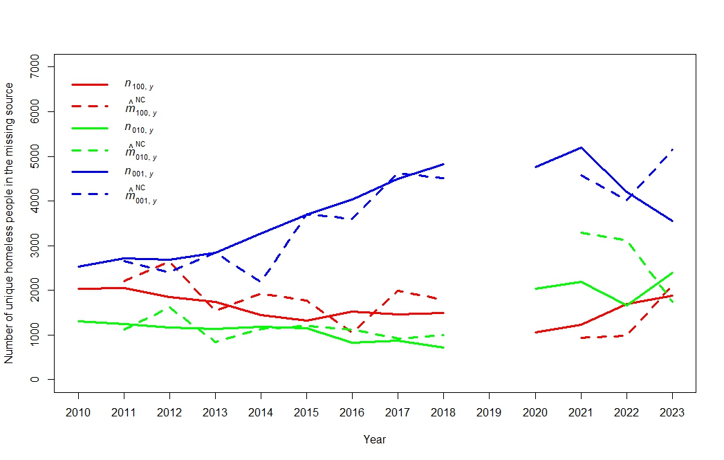
Figure 1: Observations and nowcasts of the number of homeless people that are uniquely observed in the missing sample over the periods 2010-2018 and 2020-2023.

Figure 1 shows that irrespective of the unavailable sample, the nowcasting model estimates $\hat{m}_{100,y}^{\text{NC}}$, $\hat{m}_{010,y}^{\text{NC}}$ and $\hat{m}_{001,y}^{\text{NC}}$ follow a similar trend as the observed counts $n_{100}$, $n_{010}$ and $n_{001}$ that are available later, although for some year/missing sample combinations the difference can be quite substantial.

A similar figure can be constructed with a time series of TSE estimates ($\hat{N}_{y}^{\text{TSE}}$) based on all samples and the DSE ($\hat{N}_{bc,y}^{\text{DSE}}$, $\hat{N}_{ac,y}^{\text{DSE}}$ and $\hat{N}_{ab,y}^{\text{DSE}}$) and NC ($\hat{N}_{bc,y}^{\text{NC}}$, $\hat{N}_{ac,y}^{\text{NC}}$ and $\hat{N}_{ab,y}^{\text{NC}}$) estimates based on early available samples. The samples that are used in the estimation are indicated in the subscripts. For example, $\hat{N}_{ab,}^{\text{DSE}}$ and $\hat{N}_{ab,}^{\text{NC}}$ are a DSE and NC estimate based on sample $A_{t_{1}}$ and $B_{t_{1}}$, while $C_{t_{1}}$ is missing. These series are presented in Figure 2 below.

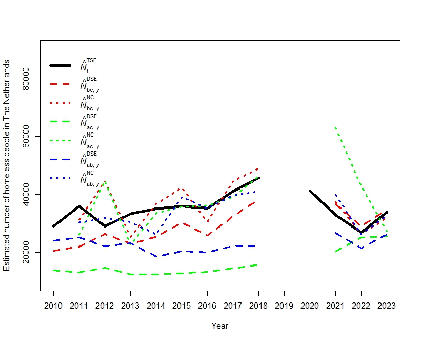
Figure 2: Estimates of the number of the total number of homeless people in The Netherlands over the periods $2010-2018$ and $2020-2023$.

Figure 2 shows that for most years the nowcasting model estimates are much closer to the TSE estimates than the DSE estimates, which suggest that in this case the nowcasting model assumption of $\lambda_{ab,(y-1)}^{AB}=\lambda_{ab,y}^{AB}$ is more reasonable than the DSE assumption $\lambda_{ab,(y-1)}^{AB}=0$. However, for some years the nowcasting model estimate can be quite bad, such as $\hat{N}_{ac,y}^{\text{NC}}$ in the years $2021$ and $2022$.

For many years it is questionable if the nowcasting model estimate is a better estimate than the TSE estimate of the previous year. In such cases a nowcast has no clear value added. To look deeper into this issue, Table 4 presents the differences between the TSE estimates with the lagged TSE estimates and nowcasting model estimates.

Table 4: Difference per year ($\times 1000$) between the TSE estimate and different estimates for each year

Year	$\hat{N}_{(y-1)}^{\text{TSE}}-\hat{N}_{y}^{\text{TSE}}$		$\hat{N}_{bc,y}^{\text{NC}}-\hat{N}_{y}^{\text{TSE}}$		$\hat{N}_{ac,y}^{\text{NC}}-\hat{N}_{y}^{\text{TSE}}$		$\hat{N}_{ab,y}^{\text{NC}}-\hat{N}_{y}^{\text{TSE}}$
2011	-6	.9	-4	.8	-9	.9	-5	.7
2012	-7	.0	15	.7	15	.6	2	.8
2013	4	.3	-8	.1	-10	.7	-2	.8
2014	1	.8	1	.6	-1	.6	-8	.9
2015	0	.9	6	.3	-0	.2	3	.1
2016	-0	.8	-4	.7	0	.9	0	.0
2017	6	.0	3	.5	-2	.2	-1	.4
2018	4	.6	3	.2	0	.6	-4	.7
2021	-8	.3	4	.6	30	.2	7	.2
2022	-6	.0	-0	.7	16	.1	-0	.6
2023	6	.9	-1	.8	-6	.5	-0	.9
Mean absolute difference	4	.5	4	.7	8	.1	3	.3

Table 4 shows that the proximity of the nowcasting model estimates and the TSE estimate clearly differs for each sample delivery order. The best results are in the last column $\hat{N}_{ab,y}^{\text{NC}}-\hat{N}_{y}^{\text{TSE}}$, which has the lowest mean absolute difference ($3.3$), which implies that in case of the homeless data the nowcasting model with sample $C_{y}$ missing gives the best results. This is a bit surprising, because Table 3 shows that sample $C_{y}$ is also the largest sample, which means that its absence should have on average a larger negative impact on the mean absolute difference than the absence of the other sources. However, an explanation of this somewhat paradoxical result can be found in Figure 3, which shows that the interaction coefficient $\hat{\mu}_{ab,y}^{AB}$ is more stable than $\hat{\mu}_{ac,y}^{AC}$ and $\hat{\mu}_{bc,y}^{BC}$, and therefore in this example the nowcasting assumption of a stable $\lambda_{ab,y}^{AB}$ is best met when sample $C_{y}$ is missing, which seems to outweigh the sample size argument.

The first column $\hat{N}_{(y-1)}^{\text{TSE}}-\hat{N}_{y}^{\text{TSE}}$ presents the difference between the current TSE and previous TSE estimate. The mean absolute difference in the last row ($4.5$) is smaller than two out of three mean absolute differences of the nowcasting models. This can be explained by the relative stability and low volatility of the TSE estimates time series. In case of a less stable or more volatile series, the mean absolute difference will be larger. This implies that in this example of the number of homeless people in The Netherlands, under a different sample delivery order it might be preferable to simply use the lagged time series, but in case of a less stable and more volatile series the nowcasting model may be a better choice.

Finally, to see if the model assumption of stable pairwise-dependencies is reasonable the TSE estimates $\hat{\mu}_{ab,y}^{AB}$, $\hat{\mu}_{ac,y}^{AC}$ and $\hat{\mu}_{bc,y}^{BC}$ over the periods $2011-2018$ and $2021-2023$ are presented in Figure 3 below.

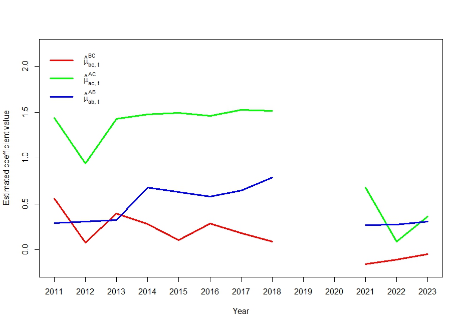
Figure 3: Coefficient estimates of $\mu_{ab,y}^{AB}$, $\mu_{ac,y}^{AC}$ and $\mu_{bc,y}^{BC}$ over the periods $2011-2018$ and $2021-2023$.

Figure 3 clearly shows three separate time series, which indicates that there is at least some stability in $\mu_{ab,y}^{AB}$, $\mu_{ac,y}^{AC}$ and $\mu_{bc,y}^{BC}$ over time. However, in some years there can be a sudden decrease or increase in the time series, for which we have no immediate explanation. These large changes correspond to the larger nowcasting errors shown in Table 4. Note that in the period $2021-2023$ the estimate for $\mu_{ac,y}^{AC}$ substantially smaller than in its estimates in the period $2011-2018$. This can be explained by the fact that sample $B_{y}$ before $2019$ is a different sample than sample $B_{y}$ after $2019$. Before $2019$ sample $B_{y}$ was a sample of homeless people who suffered from drug addictions problems and after $2019$ sample $B_{y}$ was a sample of homeless people of ex-prisoners who received reintegration support.

5 Discussion

In this paper we propose to combine dual- and triple system estimation over two periods by means of the expectation-maximisation algorithm to obtain a preliminary estimate, that we have coined a nowcast estimate. The advantage of this approach is that it allows estimation with two samples, like in DSE, but the independence assumption in DSE is replaced by a more relaxed assumption, which is that the pairwise-dependence of the first two samples is equal to the pairwise-dependence of the first two samples in the previous period. This assumption is more relaxed, because in DSE the independence assumption also implies that the pairwise dependence is equal in two periods, because in DSE the pairwise-dependence should be equal to zero all periods. This last part of the assumption is not necessary for our proposed nowcasting model. To see if the nowcasting model can be reasonably applied it is therefore advisable, when a sufficiently long time series is available, to check the stability of the interaction parameter estimates.

We applied the TSE nowcasting model to obtain nowcast estimates for the number of homeless people in The Netherlands. The model shows reasonable results in the sense that the nowcast estimates of the expected number of homeless people unique to the missing sample are quite accurate. Furthermore, the nowcasting model estimates are much more similar to the final TSE estimates than the DSE estimates, which indicates that in our example the assumption of stable pairwise-dependency is more realistic than the assumption of pairwise-independence. The accuracy of the nowcasting model is also related to the size of the missing sample. If the largest sample is missing, on average the mean absolute difference between the nowcast and TSE estimate should increase. However, in our case a stable pairwise-dependency showed to be of greater importance than the sample size of the missing sample. Finally, although the TSE nowcasting model provides reasonable results for many periods, we should note that some nowcasting model estimates can be quite inaccurate, for example the nowcasting model estimate $\hat{N}_{ac,y}^{\text{NC}}$ in the years $2021$ and $2022$, as seen in Figure 2. The reason for this inaccuracy was found in the instability of the estimated pairwise-interaction between sample $A_{y}$ and $C_{y}$ for those years. Also, because in our example the time series of TSE estimates is reasonably stable, the TSE nowcasting model does not clearly outperform the lagged time series of TSE estimates. Therefore, in cases were the time series of TSE estimates is less stable, the nowcasting model presented in this paper may be more valuable.

References

- Coumans \BOthers. (\APACyear2017) \APACinsertmetastarCoumans2017{APACrefauthors}Coumans, M\BPBIA., Cruyff, M., van der Heijden, P\BPBIG\BPBIM., Wolf, J.\BCBL \BBA Schmeets, H. \APACrefYearMonthDay2017. \BBOQ\APACrefatitleEstimating Homelessness in The Netherlands Using a Capture-Recapture Approach Estimating homelessness in The Netherlands using a capture-recapture approach.\BBCQ \APACjournalVolNumPagesSocial Indicators Research130189–212. {APACrefURL} https://doi.org/10.1007/s11205-015-1171-7 {APACrefDOI} \doi10.1007/s11205-015-1171-7 \PrintBackRefs\CurrentBib
- Dempster \BOthers. (\APACyear1977) \APACinsertmetastarDempster1977{APACrefauthors}Dempster, A\BPBIP., Laird, N\BPBIM.\BCBL \BBA Rubin, D\BPBIB. \APACrefYearMonthDay1977. \BBOQ\APACrefatitleMaximum Likelihood from Incomplete Data via the EM Algorithm Maximum likelihood from incomplete data via the em algorithm.\BBCQ \APACjournalVolNumPagesJournal of the Royal Statistical Society. Series B (Methodological)3911–38. {APACrefURL} [2024-03-21]http://www.jstor.org/stable/2984875 \PrintBackRefs\CurrentBib
- Fienberg (\APACyear1972) \APACinsertmetastarFienberg1972{APACrefauthors}Fienberg, S\BPBIE. \APACrefYearMonthDay1972. \BBOQ\APACrefatitleThe Multiple Recapture Census for Closed Populations and Incomplete Contingency Tables The multiple recapture census for closed populations and incomplete contingency tables.\BBCQ \APACjournalVolNumPagesBiometrika593591–603. {APACrefURL} https://doi.org/10.2307/2334810 {APACrefDOI} \doi10.2307/2334810 \PrintBackRefs\CurrentBib
- Lincoln (\APACyear1930) \APACinsertmetastarLincoln1930{APACrefauthors}Lincoln, F\BPBIC. \APACrefYear1930. \APACrefbtitleCalculating Waterfowl Abundance on the Basis of Banding Returns Calculating waterfowl abundance on the basis of banding returns (\BVOL 118). \APACaddressPublisherUnited States Department of Agriculture. {APACrefURL} https://doi.org/10.5962/bhl.title.64010 {APACrefDOI} \doi10.5962/bhl.title.64010 \PrintBackRefs\CurrentBib
- Lindsay (\APACyear1995) \APACinsertmetastarLindsay1995{APACrefauthors}Lindsay, B\BPBIG. \APACrefYearMonthDay1995. \BBOQ\APACrefatitleMixture Models: Theory, Geometry and Applications Mixture models: Theory, geometry and applications.\BBCQ \APACjournalVolNumPagesNSF-CBMS Regional Conference Series in Probability and Statistics5i–163. {APACrefURL} [2024-03-22]http://www.jstor.org/stable/4153184 \PrintBackRefs\CurrentBib
- Petersen (\APACyear1896) \APACinsertmetastarPetersen1896{APACrefauthors}Petersen, C\BPBIG\BPBIJ. \APACrefYearMonthDay1896. \BBOQ\APACrefatitleThe Yearly Immigration of Young Plaice Into the Limfjord From the German Sea The yearly immigration of young plaice into the Limfjord from the German Sea.\BBCQ \APACjournalVolNumPagesReport of the Danish Biological Station65–84. {APACrefURL} https://archive.org/details/reportofdanishbi06dans/page/n1/mode/2up \PrintBackRefs\CurrentBib
- Seber (\APACyear1982) \APACinsertmetastarSeber1982{APACrefauthors}Seber, G\BPBIA\BPBIF. \APACrefYear1982. \APACrefbtitleThe Estimation of Animal Abundance and Related Parameters The estimation of animal abundance and related parameters (\PrintOrdinalSecond \BEd). \APACaddressPublisherLondon: Griffin. {APACrefURL} https://archive.org/details/estimationofanim0000sebe/page/n5/mode/2up \PrintBackRefs\CurrentBib
- Wolter (\APACyear1986) \APACinsertmetastarWolter1986{APACrefauthors}Wolter, K\BPBIM. \APACrefYearMonthDay1986. \BBOQ\APACrefatitleSome Coverage Error Models for Census Data Some coverage error models for census data.\BBCQ \APACjournalVolNumPagesJournal of the American Statistical Association81338–346. {APACrefURL} https://doi.org/10.2307/2289222 {APACrefDOI} \doi10.2307/2289222 \PrintBackRefs\CurrentBib
- Zwane \BBA van der Heijden (\APACyear2007) \APACinsertmetastarZwane2007{APACrefauthors}Zwane, E\BPBIN.\BCBT \BBA van der Heijden, P\BPBIG\BPBIM. \APACrefYearMonthDay2007. \BBOQ\APACrefatitleAnalysing capture–recapture data when some variables of heterogeneous catchability are not collected or asked in all registrations Analysing capture–recapture data when some variables of heterogeneous catchability are not collected or asked in all registrations.\BBCQ \APACjournalVolNumPagesStatistics in Medicine261069–1089. {APACrefURL} https://doi.org/10.1002/sim.2577 {APACrefDOI} \doi10.1002/sim.2577 \PrintBackRefs\CurrentBib
- Zwane \BOthers. (\APACyear2004) \APACinsertmetastarZwane2004{APACrefauthors}Zwane, E\BPBIN., van der Pal-de Bruin, K.\BCBL \BBA van der Heijden, P\BPBIG\BPBIM. \APACrefYearMonthDay2004. \BBOQ\APACrefatitleThe multiple-record systems estimator when registrations refer to different but overlapping populations The multiple-record systems estimator when registrations refer to different but overlapping populations.\BBCQ \APACjournalVolNumPagesStatistics in medicine232267–81. {APACrefURL} https://doi.org/10.1002/sim.1818 {APACrefDOI} \doi10.1002/sim.1818 \PrintBackRefs\CurrentBib