Inspiral-merger-ringdown
waveforms in Einstein-scalar-Gauss-Bonnet
gravity within the
effective-one-body formalism
Abstract
Gravitational waves (GWs) provide a unique opportunity to test General Relativity (GR) in the highly dynamical, strong-field regime. So far, the majority of the tests of GR with GW signals have been carried out following parametrized, theory-independent approaches. An alternative avenue consists in developing inspiral-merger-ringdown (IMR) waveform models in specific beyond-GR theories of gravity, by combining analytical and numerical-relativity results. In this work, we provide the first example of a full IMR waveform model in a beyond-GR theory, focusing on Einstein-scalar-Gauss-Bonnet (ESGB) gravity. This theory has attracted particular attention due to its rich phenomenology for binary black-hole (BH) mergers, thanks to the presence of non-trivial scalar fields. Starting from the state-of-the-art, effective-one-body (EOB) multipolar waveform model for spin-precessing binary BHs SEOBNRv5PHM, we include theory-specific corrections to the EOB Hamiltonian, the metric and scalar energy fluxes, the GW modes, the quasi-normal-mode (QNM) spectrum and the mass and spin of the remnant BH. We also propose a way to marginalize over the uncertainty in the merger morphology with additional nuisance parameters. Interestingly, we observe that changes in the frequency of the ringdown waveform due to the final mass and spin corrections are significantly larger than those due to ESGB corrections to the QNM spectrum. By performing Bayesian parameter estimation for the GW events GW190412, GW190814 and GW230529181500, we place constraints on the fundamental coupling of the theory ( at confidence). The bound could be improved by one order of magnitude by observing a single “golden” binary system with next-generation ground-based GW detectors. Our model can be used to improve constraints on modifications of GR with upcoming GW observations, and to provide forecasts for future GW detectors on the ground and in space.
I Introduction
The observations of gravitational waves (GWs) from coalescing binary systems [1, 2, 3, 4, 5, 6] with the LIGO and Virgo detectors [7, 8] have for the first time allowed us to test Einstein’s theory of General Relativity (GR) in the highly nonlinear and dynamical regime [9, 10, 11, 12, 13]. Near-future upgrades to the LIGO, Virgo and KAGRA [14] (LVK) interferometers, and upcoming detectors on the ground, Einstein Telescope (ET) and Cosmic Explorer (CE) [15, 16], and in space (LISA) [17], will significantly increase the number of detected sources, some of which will be observed with signal-to-noise ratios (SNR) reaching thousands, allowing for tests of GR with exquisite precision (see, e.g., Ref. [18]).
One can adopt either a theory-independent or theory-specific approach to testing GR. Theory-independent tests modify GR waveform models by introducing some generic, parameterized deviations, which are constrained by comparing the waveform templates with an observed GW signal (a non-exhaustive list includes Refs. [19, 20, 21, 22, 23, 24, 25, 26, 27, 28, 29, 30, 31]), or look for consistency between the signal, or portions of the signal, and the data, without invoking any parametrization of the deviations [32, 33, 34, 35]. Theory-specific tests (see, e.g., Refs. [36, 37, 38, 39, 40]) use instead waveforms predicted in a particular alternative theory of gravity and aim at estimating its underlying physical parameters. So far, the majority of tests of GR with GWs have been carried out following a theory-independent approach. While theory-independent tests can, in principle, constrain a wide range of alternative theories, parameterized deviations are not unique, and degeneracies among different deviation parameters complicate constraining multiple of them at the same time unless specific combinations are selected [41]. Moreover, there is no guarantee that parameterized deviations can represent the potentially infinite landscape of beyond-GR theories (see Ref. [42] for an attempt to address this issue). Furthermore, although such tests are valuable in identifying possible deviations from GR, they do not necessarily inform us about the new physics at play. Thus, it is relevant to develop, both analytically (see, e.g., Refs. [43, 44, 45, 46, 47, 48, 49, 50, 51, 52, 53, 54, 55, 56, 57, 58, 59, 60, 61, 62, 63, 64, 65, 66, 67, 68, 69, 70, 71, 72]) and numerically (see, e.g., Refs. [73, 74, 75, 76, 77, 78, 79, 80, 81, 82, 83, 84, 85, 86, 87, 88, 89, 90, 91, 92, 93, 94, 95, 96, 97, 98, 99, 100, 101, 102, 103, 104, 105]), waveform models in specific beyond-GR theories of gravity.
One avenue to conduct theory-specific tests is to develop accurate inspiral-merger-ringdown (IMR) waveform models in alternative theories of gravity, combining analytical and numerical-relativity (NR) results, as done in GR [106, 107, 108, 109, 110, 111, 112]. In this work, we provide the first example of a full IMR waveform model featuring analytical beyond-GR corrections. We focus on Einstein-scalar-Gauss-Bonnet (ESGB) theories, which supplement GR with a massless scalar field coupled to the Gauss-Bonnet scalar , with a coupling of the form in the action. These theories have attracted particular attention, thanks to their rich phenomenology for black holes (BHs) with scalar “hair” [113, 114, 115, 116, 117, 118, 45, 119, 120, 121, 122, 123, 124, 61, 65]. In particular, for certain functions , BHs can undergo spontaneous [125, 126, 127, 128, 129, 130, 131] or dynamical [86, 93, 94, 132, 72] (de)scalarization phenomena analogous to those predicted for neutron stars (NSs) in scalar-tensor (ST) theories of gravity [44, 74, 76, 77]. Different methods have been proposed to include dynamical scalarization in waveform models [133, 134, 135, 136]. Recent progress in ESGB gravity was made to obtain inspiral waveforms within the post-Newtonian (PN) and effective-one-body (EOB) formalisms [61, 68, 62, 65, 137], to calculate quasi-normal-mode (QNM) frequencies of rotating BHs at second order in a small-spin expansion [50, 63, 66] and very recently for large spins [138, 139], and to numerically simulate binary black holes (BBHs) [78, 80, 81, 84, 85, 83, 87, 88, 89, 91, 92, 101, 100, 99, 102, 103], binary neutron stars (BNSs) [140, 141] and neutron star-black hole (NSBH) binaries [104].
The most commonly used methods to build complete IMR waveform models for compact binaries in GR are the NR surrogate [142, 143, 144], phenomenological [145, 146, 147, 148, 149, 150] and EOB [108, 151, 152, 153, 154, 155] frameworks. EOB waveform models combine and resum information from several analytical approximation methods (PN, post-Minkowskian, gravitational self-force) with a physically motivated ansatz for the merger, and BH perturbation theory for the ringdown, and are made highly accurate through calibration with NR simulations. There are currently two state-of-the-art families of EOB waveform models: SEOBNR (see, e.g., Refs. [156, 157, 158, 159, 160]) and TEOBResumS (see, e.g., Refs. [161, 162, 163, 164, 165]). Here, we focus on the former.
In this work, we start from the state-of-the-art EOB waveform model SEOBNRv5PHM [157], which includes effects of higher harmonics and spin precession, and we include ESGB corrections to the EOB Hamiltonian, the GW and scalar-energy fluxes, the spherical-harmonic GW modes, the QNM spectrum, and the mass and spin of the remnant BH. To account for the uncertainty in merger features that may only be determined when further NR simulations are available in ESGB gravity, we use parametrized deviations inspired by the pSEOBNR pipeline [25, 30, 166], interpreted as nuisance parameters. We implement our waveform model within the pySEOBNR Python package [167], a code recently developed to construct, calibrate and validate new EOB waveform models with efficiency and flexibility. We refer to our new model with the name SEOBNRv5PHMESGB.
In a second step, we use SEOBNRv5PHMESGB to provide constraints on the coupling length of the dilatonic theory by analyzing the GW events GW190412, GW190814 and GW230529181500 (to which we will refer as GW230529 for brevity) through Bayesian inference, and compare our results to the literature. We improve previous analyses [168, 169, 170] by including ESGB corrections to the waveform for the entire coalescence, and as a consequence, by analyzing the complete signal rather than restricting to its inspiral phase. Our results for GW190814 are in agreement with Refs. [168, 170], with a bound on their coupling length . For GW230529, which currently places the best constraint on this theory, we obtain . This is consistent with Refs. [171, 172], which obtain a bound on ranging from to depending on the waveform approximant employed. On the other hand, we obtain from GW190412 the bound , roughly a factor smaller than previous analyses [168]. This is consistent with the larger mass of the source of GW190412, resulting in a higher relative SNR in the late-inspiral stage, for which we are including additional corrections. Stacking the posteriors of the three events, we obtain a combined bound , depending on whether we include the merger-ringdown portion of the signal or not. Our waveform templates also allow for Bayesian–model-selection studies, to address whether the GR hypothesis is favored over a specific modified gravity theory in describing GW data [173]. We compute Bayes factors between the GR and ESGB hypotheses, finding the three analyzed events to be consistent with GR.
The paper is organized as follows. In Sec. II we introduce ESGB theories and their PN description. In Sec. III, we review the structure of the EOB Hamiltonian in GR, and include its ESGB corrections at 3PN. In Sec. IV we present the ESGB metric and scalar energy fluxes on circular orbits and at relative 2PN and 2.5PN orders. In Section V, we recall the structure of the IMR spherical-harmonic waveform modes in GR, and obtain their ESGB corrections. In Sec. VI we present our results on waveform morphology and Bayesian parameter estimation. In Section VII, we summarize our main conclusions and discuss future work. Various technical details are relegated to the appendices. In Appendix A we present a dictionary relating quantities in the Einstein and Jordan frames. In Appendix B we recall the ESGB corrections to the EOB metric. In Appendix C we gather factors entering the metric modes. In Appendix D we list the coefficients of the scalar flux. Finally, in Appendix E we provide the spherical-harmonic scalar modes at relative 1.5PN order. Throughout this paper we use geometrical units ().
II Einstein-scalar-Gauss-Bonnet reminder
II.1 ESGB and ST gravity
We study the class of theories described by the Einstein-frame action [61, 43]
| (1) |
where is the Ricci scalar, is the metric determinant, and is the Gauss-Bonnet scalar, where and are the Riemann and Ricci tensors, respectively. The integral over a four-dimensional spacetime is a boundary term [174]. As for matter fields , they couple minimally to the Jordan metric . The length and the dimensionless functions and specify the theory. We recover ST theories in the limit or if is constant, and GR if moreover (and ) is constant.
To model compact bodies, we use the phenomenological treatment initiated in Refs. [175, 43] in ST theories, and describe them as point particles:
| (2) |
where and is the worldline of particle . The constant GR mass becomes a function that depends on the internal structure of body and on the value of the scalar field at .
In this paper, we will refer to the theory with action (1) as ESGB gravity, but note that ST theories are included as a particular subcase.
| 0PN | |
| 1PN | |
| 2PN | |
| 3PN | |
| (Anti) symmetry | with |
| Mean value | |
II.2 Post-Newtonian framework
We focus on the dynamics of compact binary systems on bound orbits. When the relative orbital velocity is small and the gravitational field is weak, the motion can be studied in the PN framework.111We denote by PN the corrections to the Newtonian dynamics, with the system’s relative orbital velocity, the total mass, and the orbital radius. To this aim, the field equations of the theory (1) with the substitution (2) are solved iteratively around a flat metric , and a constant scalar field background , where is imposed by the binary’s cosmological environment.
From now on, a superscript denotes a quantity evaluated at . We consider a binary system with , and define its total mass, reduced mass, and the dimensionless ratios
| (3) |
The functions and , describing bodies and , can then be further expanded at 3PN by introducing the following quantities:
| (4a) | ||||
| (4b) | ||||
| (4c) | ||||
| (4d) | ||||
and their counterparts for body . We also introduce the notation .
The ESGB corrections included in this work will depend only on the theory-dependent product and on ten body-dependent parameters: the masses of bodies and and their logarithmic derivatives (4) at infinity (i.e., at ), via the combinations gathered in Table 1. We recover ST theories in the limit , and GR when moreover and are constants: then, Eqs. (4) and their -counterparts are zero, so that only is nonzero in Table 1.
Note that differs from its original definition in Ref. [68] by a factor . This factor originates from a typographical error in Ref. [58], which the author communicated to us, after it was pointed out in Ref. [68] [cf. Sec. II.B there] that the terms in Ref. [58] depending on or (in the Einstein frame) should be revised. In practice, the factor in Eq. (A3) of Ref. [58] must be replaced by . The terms depending on in Ref. [58] still require revision, and they enter the present paper via in Eq. (85b).
II.3 The example of dilatonic ESGB gravity
The quantities (4) can be calculated once the theory and the bodies are specified. In ST theories, they were derived numerically for NSs in Refs. [43, 177, 44, 44, 178]. They were also calculated in ESGB models for BHs, including spontaneously and dynamically scalarized ones, in Refs. [61, 65, 72].
For the sake of illustration, we will apply our results explicitly to the dilatonic ESGB theory222We translate between our conventions and those of Refs. [168, 170] by setting and .
| (5) |
for which the action (1) becomes invariant under the simultaneous redefinitions and , where is a constant. In this theory, the quantities (4) were derived analytically and numerically for nonspinning BHs in Refs. [61, 65]. Given a BH , they are functions of two parameters only: , which we set here to zero without loss of generality, using the symmetry of the theory; and the dimensionless ratio , where the bound ensures the regularity of the horizon [65].
In this paper, we will describe BBHs and NSBH binaries as follows. For BBHs, we use the analytical, nonperturbative -Padé approximant of (and ) discussed in Sec. III.B of Ref. [65], which exhibits remarkable agreement with its numerical counterpart. We then infer , and (and their counterparts for BH ) using Eqs. (4b)–(4d). Since , it is sufficient to impose the horizon regularity bound on BH .
By contrast, Eqs. (4) were so far not calculated for NSs in the dilatonic ESGB theory. However, we can describe NSBH binaries at leading order in the small- approximation. We indeed have, for a BH [61, 65],
| (6) |
At this order, the theory reduces to the shift-symmetric ESGB model [61], in which NSs are known to carry no scalar monopole [46, 179]. Since Eq. (4a) is proportional to the latter [43, 54], we conclude that for a NS [170],
| (7) |
In the small- approximation, the contributions from , and (and their counterparts for NS ) are subleading and can be discarded, because they only enter the dynamics via the combinations gathered in Table 1, which are already quadratic in or .
The ST two-body Lagrangian was derived at 1PN by Damour and Esposito-Farèse [43], at 2PN by Mirshekari and Will [47] and at 3PN by Bernard [58]. It was then generalized by Julié and Berti, who derived its ESGB corrections in Ref. [61]. The resulting conservative dynamics was included within an EOB Hamiltonian at 2PN by Julié and Deruelle [52, 53, 68], and at 3PN by Julié et al. [68]; see also Jain et al. [67, 69] in the ST limit. We include the main results as corrections to the SEOBNRv5PHM Hamiltonian in Sec. III.1, and extend those works to the radiative sector in Secs. III.2, IV and V.
III Effective-one-body Hamiltonian and equations of motion
III.1 The EOB Hamiltonian
In the EOB formalism [108, 151, 152, 153, 154], the two-body Hamiltonian in the center-of-mass frame is mapped, through canonical transformations, to the effective Hamiltonian of a test mass in a deformed BH spacetime, the deformation parameter being the symmetric mass-ratio , as [108]
| (8) |
where . For nonspinning (noS) binaries, the motion is planar and we can use polar coordinates . We introduce the following reduced variables:
| (9) |
The effective Hamiltonian then takes the form
| (10) |
where we use the tortoise-coordinate instead of to facilitate the numerical integration of the equations of motion close to merger. Indeed, diverges when approaching the zero of , while is finite [180, 181]. For nonspinning binaries, the tortoise-coordinate is defined by
| (11) |
and the conjugate momentum is
| (12) |
In the general relativistic SEOBNRv5PHM Hamiltonian [159], the potentials and are based on the 5PN results of Refs. [182, 183], which are complete modulo two unknown constants at 5PN order, denoted and there. In SEOBNRv5PHM, one sets and replaces the 5PN coefficient in , with the exception of the part proportional to , by a function calibrated to NR simulations [156]. The potential uses the full 5.5PN expression of Refs. [183, 184], once is traded for by inverting Eq. (12) at the same order. This potential is known to , thus accounting for nonlocal-in-time “tail” effects (entering at 4PN in GR) to eighth order in the binary’s orbital eccentricity. The complete potentials are given explicitly in Ref. [159]
To include the ESGB effects up to 3PN order in the SEOBNRv5PHM Hamiltonian, we follow the prescription of Ref. [68]:
-
1.
Formally replace by , defined as
(13) at all PN orders in the potentials , and , where is defined in Table 1.
- 2.
We note that the potential in Ref. [68] is a function of , and it is linked to our potentials through . Since it was calculated at leading PN order, our are the same as those presented in Ref. [68]. The ESGB corrections in Eq. (14c) are known to , which amounts to including the ESGB “tail” effects to sixth order in the eccentricity. These effects already appear at 3PN, due to (dipolar) scalar radiation that is absent in GR.
To improve the accuracy of the model against NR waveforms in the GR limit, we resum using a (1,5)-Padé approximant with respect to [152, 185, 186, 161, 156]
| (15) |
which features a simple zero (by construction), consistently with the Schwarzschild metric recovered in the GR, test-mass limit. We also resum as a (2,3)-Padé approximant [156, 187]
| (16) |
which remains numerically close to the Schwarzschild value 1 in the range . Note that the ESGB corrections in the and potentials are added before performing the Padé resummations (which are the same as in GR) so that the potentials remain qualitatively consistent with their GR counterparts as is increased.
For generic nonzero spins, the SEOBNRv5PHM Hamiltonian takes inspiration from that of a test mass in a deformed Kerr background [153, 188, 189, 159]. It includes spin-orbit (SO) information up to next-to-next-to-leading order (NNLO), spin-spin (SS) information to NNLO, as well as cubic- and quartic-in-spin terms at leading order (LO), corresponding to the 4PN order for generic, precessing spins. For efficiency, some spin-precession effects are analytically averaged out over circular orbits [159]. The tortoise coordinate is also extended as
| (17) |
with , where and are the dimensionless spins of the bodies projected along the orbital angular momentum at Newtonian order. More details and full expressions can be found in Refs. [159, 156, 157]. We do not add any ESGB correction in the spin contributions to the Hamiltonian, because they are currently unknown.
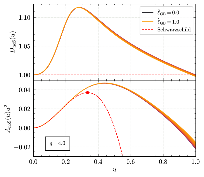
The ESGB corrections to the EOB potentials in Eqs. (15) and (16) are valid for arbitrary choices of the functions and entering the action (1). They can be specified to a particular theory and compact binary once the corresponding values of the quantities (4) are given. As an explicit illustration, we show in Fig. 1 the potentials and for a nonspinning BBH with in the dilatonic ESGB case (5), varying the rescaled Gauss-Bonnet coupling [cf. Eq. (3)] in the range . The value is just below that at which the BH becomes a naked singularity. Adding back the units, this corresponds to a coupling , in the notation of Ref. [170]. We note that the peak of corresponds to the value of at the effective light-ring. While the differences in may seem small, especially below , we recall that can still lead to significantly different conservative dynamics [187], as is the case here.
III.2 The EOB equations of motion and radiation-reaction force
For nonspinning binaries or in the spin-aligned case, the SEOBNRv5PHM equations of motion are given by Eqs. (15) of Ref. [156]. They read:
| (18) |
where the dot indicates a derivative with respect to , while and . The radiation reaction (RR) force is computed as [154]
| (19) |
where is the reduced orbital frequency, and is the energy flux radiated by the binary on quasi-circular orbits. The metric flux is obtained by summing over the contributions of the factorized metric modes [180, 186, 155, 190], which we will define in Sec. V.1, that is
| (20) |
where is the distance to the source. In ESGB theories, we have to account for an additional contribution to the flux from the scalar field,
| (21) |
which we will discuss in Sec. IV.2. In the following, we express in terms of , and insert the result back into the system (18).
In the spin-precessing case, the SEOBNRv5PHM model uses the same equations of motion as in Eqs. (18) in the co-precessing frame, in which the GW radiation resembles that of an aligned-spin binary [191, 192, 193, 194, 195], together with separate PN-expanded evolution equations for the spins and angular momentum inferred from [159, 157]. For this work, we employ the same description of the precession dynamics as in the SEOBNRv5PHM model and refer the reader to Ref. [159] and Sec. II of Ref. [157] for more details. We point out that in the future, the spin and angular momentum evolution equations should be generalized to account for their ESGB corrections.
IV Gravitational radiation in ESGB gravity
In this section, we adopt the conventions of Refs. [196, 197], and define the metric perturbation:
| (22) |
whose indices are manipulated with the Minkowski metric. Let us introduce a Cartesian orthonormal basis . In the center-of-mass frame of a spin-aligned binary, the relative motion is planar and we set the source position as . We locate the observation point with spherical coordinates, such that . When , the metric waveform is the transverse, traceless part of the metric perturbation,
| (23) |
where and . Finally, we introduce the polarization vectors and and define:
| (24a) | ||||
| (24b) | ||||
which can in turn be decomposed in spin-weighted spherical harmonics of weight ,
| (25) |
IV.1 Spherical-harmonic metric modes at 2PN
In ST theories, the metric waveform (23) was derived for nonspinning binaries at 0PN by Damour and Esposito-Farèse [43] and at 2PN by Lang [48, 49] relatively to the quadrupolar order. The corresponding metric modes were then inferred by Sennett et al. in Ref. [51] for circular orbits. The corrections beyond ST from the Gauss-Bonnet coupling were calculated at leading PN order by Shiralilou et al. [198, 62], but they enter at 3PN. This means that the metric modes are complete only at 2PN in ST and ESGB gravity, an order at which their expressions are the same. Rather, they differ by the specific values taken by the quantities (4).
Yet, the results in Ref. [51] were presented using another, Jordan-frame formulation of ST theories based on a set of Brans-Dicke-inspired parameters.
To recover the conventions of the present paper, we must proceed as follows:
- 1.
-
2.
Notice that Ref. [51] uses a coordinate system such that the Jordan metric is Minkowski at infinity, . By contrast, we use here coordinates such that . The coordinate systems are thus related by
(26) with . This means that , , and the orbital velocity entering Ref. [51] must be rescaled as , , and .
-
3.
Observe that Ref. [51] studies the perturbation of where is the scalar field in the Jordan frame. This conformal metric identifies to our given the coordinate change above. The perturbation (22) also differs from that of Ref. [51] by an overall minus sign. However, their polarization vectors are and , so that our and are the same.
In harmonic coordinates such that , the metric waveform exhibits a logarithmic correction to its decay, due to tail effects at 1.5PN [48, 49]. To eliminate it, we can introduce the radiative time
| (27) |
where is an arbitrary length. The ESGB metric modes then read, at 2PN and in the radiative coordinate system :
| (28) |
where
| (29) |
with, recall, [cf. below Eq. (18)], and where
| (30) |
where is Euler’s constant. The effective phase (30) was first introduced in GR to factor out -dependent tail corrections to the modes [199], and it is now dressed-up by the scalar field effects. As for the dimensionless quantities , we gather their explicit expressions in Appendix C. Note that the orbit being planar, we have by symmetry [196]
| (31) |
where denotes complex conjugation. Thus, it is sufficient to present the modes with .
In Sec. V.1, we shall resum the modes (28) by rewriting them in a factorized form , allowing in turn to compute the metric flux [43, 200] (cf. also Refs. [60, 56, 62]),
| (32) |
where . This flux formula returns Eq. (20) on circular orbits, given the orthogonality of the spherical harmonics , the contribution of each mode being the same as that of its counterpart .
IV.2 Scalar flux at relative 2.5PN order
In ST theories, the scalar waveform
| (33) |
was derived for nonspinning binaries at 2PN by Lang [49] and at 2.5PN by Bernard et al. [64] relatively to the (scalar) dipolar order. The decomposition of on spherical harmonics was performed in Ref. [64], but the associated scalar modes are presented there through 1.5PN only. In this paper, we thus start from the scalar flux itself, which was derived at 2.5PN in Ref. [64]. As for the corrections beyond ST from the Gauss-Bonnet coupling to the scalar flux, they were calculated at leading PN order by Shiralilou et al. [198, 62], but they enter at 3PN, an order at which even the ST subcase is unknown.
Once again, the results in Refs. [49, 64] were presented using the Jordan-frame formulation of the theory.
We recover our conventions as follows:
- 1.
- 2.
- 3.
As a result of this procedure, the scalar flux formula in Refs. [49, 64] becomes
| (34) |
which coincides with our Einstein-frame definition, cf. also Refs. [43, 56, 60]. For circular orbits, the ESGB scalar flux then reads:
| (35) |
where was defined in Eq. (29), and where the lengthy expressions of the coefficients are relegated to Appendix D. To make the comparison with the metric flux transparent, the labels PN are here relative to the quadrupolar order.
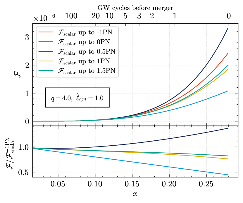
We point out that is proportional to . Thus, when restricted to the dipolar order, the scalar flux vanishes for symmetric binaries. In Fig. 2, we show the behavior of the scalar flux (IV.2) truncated at successive PN orders, as a function of . As an illustration, we consider a BBH with and in the dilatonic ESGB theory (5). The curves terminate at merger, taken as the peak of the mode amplitude when all PN orders of the scalar flux contribute to the binary’s evolution. We also show the corresponding number of GW cycles. The ratio between the scalar flux truncated at different PN orders and the leading order -1PN term highlights the poor convergence of the low PN order contributions in the late inspiral, which seems, however, improved when including higher-order PN corrections. We leave the comparison of potential resummation methods for the scalar flux to future work, when more NR waveforms become available in ESGB gravity.
For completeness, we present in Appendix E the decomposition of the scalar waveform in spherical harmonics, once translated in our Einstein-frame conventions. As explained below Eq. (33), we do not infer the scalar flux from these modes, because the result would be one PN order lower than in Eq. (IV.2).
V EOB inspiral-merger-ringdown metric waveform in ESGB gravity
In the EOB framework, the metric modes defined in Eq. (25) are decomposed into inspiral-plunge and merger-ringdown modes. The SEOBNRv5PHM model includes the modes (2,2), (2,1), (3,3), (3,2), (4,4), (4,3) and (5,5) in the co-precessing frame. We have:
| (36) |
where is the peak time of the -mode amplitude () for all the modes except , for which it is taken as the peak time of the mode minus [156]. From now on, we shall refer to as the merger time. Note that the other modes with are known in their factorized form (cf. below), but they are only used to compute the fluxes until merger.
In GR, is suitably chosen to agree with the corresponding time in NR simulations. Specifically, in the SEOBNRv5PHM model, one defines
| (37) |
where is the time at which reaches the inverse radius of the Kerr innermost stable circular orbit (ISCO) [201] with the mass and spin of the remnant BH, as predicted by NR fitting formulas [202, 203]. The calibration parameter is determined via comparisons to NR simulations [156]. In this work, we also use Eq. (37), formally replacing by its ESGB expression (13), to determine the merger-ringdown attachment time. We note that is affected by ESGB corrections, as they give rise to differences in the orbital dynamics, but we don’t include additional corrections to , which should be determined from NR simulations in ESGB gravity.
V.1 Inspiral-plunge modes
The inspiral-plunge EOB modes can be written as
| (38) |
where is a factorized, resummed form of the PN-expanded metric modes for aligned-spin binaries on circular orbits [180, 155, 190], while is the non-quasi-circular (NQC) correction [204] which does not enter the flux (20) in the SEOBNRv5PHM model. More precisely, the factorized metric modes are defined as
| (39) |
In GR, the first factor is the mode at leading PN order (called Newtonian). Its explicit expression can be found in Refs. [155, 190] for all , with an overall minus sign compared to our conventions. The second factor takes inspiration from the Regge-Wheeler-Zerilli equation sourced by a test mass , on circular orbits of the Schwarzschild spacetime of mass [155]. Depending on the parity of , it is either identified to the (reduced) effective energy of the EOB framework, or to the orbital angular momentum, normalized by its Newtonian value on circular orbits:
| (40) |
Here, and we recall that was introduced below Eq. (18). The third factor resums leading logarithms entering the tail contributions [205]:
| (41) |
where is the Euler gamma function, while is proportional to the binary’s resummed EOB energy. The constant is the same as that entering Eq. (30). In GR, it is usually set to , where is Euler’s number, to reproduce the correct test-particle limit waveforms [190]. The remaining factor depends on an amplitude and a phase , whose PN expansions in can be determined by identifying order-by-order the mode to its resummation on circular orbits.
The variable can be traded for in to gather relativistic corrections sourced by the binary’s Arnowitt-Deser-Misner (ADM) mass [155]. For even, or for nonspinning binaries, is further resummed as to reduce the magnitude of the 1PN coefficient, which grows linearly with .
By contrast, for odd, the spins deserve a particular treatment. Indeed, the procedure above yields spin contributions to inversely proportional to [cf. Eq. (3)], thus making ill-defined in the equal-mass case. This issue traces back to being zero when at Newtonian order, while some of its spin contributions, entering at subleading PN orders, are not. We thus adopt the treatment of Refs. [190, 206, 207], and redefine the amplitude and phase as follows:
| (45) |
| (49) |
where and are inferred from the nonspinning limit of and , while the additive constant reabsorbs their spin contributions, by expanding the (complex) exponential in Eq. (39). The amplitude and phase being replaced by their “barred” versions, Eq. (39) has a non-ambiguous equal-mass limit, because the terms inversely proportional to only enter (and not ), which is multiplied by .
The SEOBNRv5PHM model also incorporates information from second-order self-force (2GSF) [208, 209] in the GW mode amplitudes and radiation-reaction force, by introducing new calibration parameters in the coefficients and matching them to the 2GSF energy-flux multipolar data for quasicircular nonspinning BBHs [158]. The explicit expressions of and used in the SEOBNRv5PHM model are provided in Appendix B of Ref. [156].
The steps described above can now be generalized to ESGB theories, starting from the 2PN metric modes discussed in Sec. IV.1 [cf. also Appendix C]. To do so, we must Taylor-expand and [defined in Sec. III.1] at 1PN, as well as at 2PN on circular orbits. Now, observe that when is odd, the modes defined in Eq. (28) and Appendix C are imaginary and proportional to at Newtonian order. However, some real ESGB corrections, entering at subleading PN orders, are not. The situation is reminiscent of that with spins, and thus, we shall treat ESGB effects in a similar fashion.
More explicitly, we include the ESGB corrections to the metric modes up to 2PN within SEOBNRv5PHM as follows:
- 1.
-
2.
For odd, normalize by its Newtonian value on circular orbits in ESGB gravity, that is
(50) -
3.
In and and in the nonspinning parts of and , formally replace by [cf. Eq. (29)], and by
(51) -
4.
Deform the resulting amplitude and phase by ESGB corrections:
(55) (59)
At 2PN, the modes with contribute, and we find that the nonzero ESGB corrections read:
| (60a) | ||||
| (60b) | ||||
| (60c) | ||||
| (60d) | ||||
| (61) |
| (62a) | ||||
| (62b) | ||||
| (62c) | ||||
We do not add any ESGB correction in the spin contributions to the phase and amplitude, because they are currently unknown.
The remaining factor in the inspiral-plunge modes (38) is the NQC correction and reads
| (63) | ||||
This factor guarantees that the modes’ amplitude and frequency agree with NR input values, given by NR fits, at the matching point . In practice, one first solves for the binary’s trajectory to infer . Second, one fixes the 5 constants , , , , by requiring that the amplitude of the EOB modes and its first two derivatives, and the frequency of the EOB modes and its first derivative, are the same as that of the NR modes at the matching point [207, 210, 156]. In particular, the NQC correction enforces that the (2,2)-mode’s derivative vanishes (i.e., it peaks) at the merger time defined in Eq. (37). Since the factorized modes include ESGB corrections, the five constants above are changed so that the inspiral-plunge waveform (38) still matches the NR predictions in GR at . In Sec. V.2, we shall discuss how to relax this assumption.
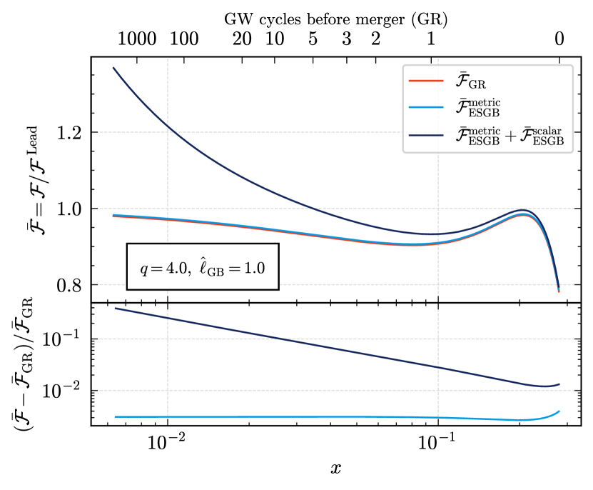
In Fig. 3, we show the GR and ESGB fluxes normalized by the leading order GR contribution
| (64) |
considering only the ESGB corrections to the metric flux, or also adding the scalar flux. As in Fig. 2, we consider a binary with and in the dilatonic theory (5). Looking at the fractional difference between the ESGB fluxes and the GR flux, we note that the difference in the metric flux at low frequencies is constant with (e.g., at leading PN order), and is due to the replacement of with as in Eq. (29), while the difference when including the scalar flux increases at low frequencies as , due to the dipolar -1PN term.
V.2 Merger-ringdown modes
For the merger-ringdown waveform in ESGB, we assume the same phenomenological ansätze as in GR [211, 210, 212, 156], but introduce an appropriate parameterization for the modes’ amplitude and frequency [25, 30, 166]. We also use the QNMs derived recently in ESGB gravity [138].
More precisely, for all harmonics except and , which exhibit post-merger oscillations due to mode-mixing [213, 214], the merger-ringdown GR waveform employs the following ansatz [215, 216, 210, 156]:
| (65) |
where is the complex frequency of the least-damped QNM (with overtone number zero) of the remnant BH. The corresponding oscillation frequency and damping time read
| (66a) | ||||
| (66b) | ||||
The functions and are given by [156]:
| (67a) | ||||
| (67b) | ||||
where is the phase of the inspiral-plunge mode at [cf. below Eq. (36)]. The coefficients and () are constrained by the requirement that the amplitude and phase of are continuously differentiable at , while the coefficients and are obtained through fits to a large set of aligned-spin NR waveforms, spanning mass ratios up to 20 and spins up to 0.998, and BH perturbation-theory merger-ringdown waveforms with mass ratio 1000. For the and modes, the mode-mixing behavior is modeled by applying the previous construction to the spheroidal harmonics [217] and , which feature a monotonic amplitude and frequency evolution [218]. The and modes are then obtained by combining the and modes with the and modes using the appropriate mixing coefficients [219].
In the SEOBNRv5PHM model [156, 157], the complex QNM frequencies in GR are obtained for each harmonic as a function of the BH’s (dimensionless) final mass and spin using the qnm Python package [220]. Note that the qnm package provides , as a function of the final spin , so in Eq. (65) we use
| (68) |
The BH’s mass and spin are in turn computed using the fitting formulas of Refs. [202] and [203], respectively.
We now describe how we account for ESGB effects in the merger-ringdown modes. For the merger, as reminded on Sec. V.1, the NQC corrections impose that the modes’ amplitude and frequency agree with fits to NR waveforms in GR. In recent years, there has been a significant effort to produce NR simulations in beyond-GR theories [79, 82, 90, 95, 97, 98], with a few examples of NR evolutions of BBHs in ESGB gravity [80, 85, 83, 94, 91, 99]. For example, Ref. [91] found a negligible effect on the GW amplitude at merger with varying ESGB coupling, in contrast with the large effect found in the order-reduced simulation of Ref. [83], possibly due to the presence of secularly growing errors present in the latter perturbative approach (see [103] for a detailed comparison of different numerical approaches). In any case, making parameter-space fits (calibration) of such merger properties, as done in GR, requires a large number of NR waveforms, which are not yet available.
To account for possible deviations in the waveform at merger, we take inspiration from the parametrized SEOBNR approach (pSEOBNR) [25, 30, 166], and introduce fractional deviations to the NR predictions in GR for the amplitude and frequency at for each mode. These deviations parameterize our ignorance of the merger morphology with extra nuisance parameters, to be marginalized over in parameter estimation. Given this idea, we want the corrections to vanish in the GR limit, so we rescale them as
| (69a) | ||||
| (69b) | ||||
where the dependence is inspired by the scaling of the PN corrections in the inspiral modes in the small- regime. In turn, this rescaling changes the values taken by the constants and entering Eqs. (63) and (67), respectively. The -dependence in Eqs. (69), and how the merger morphology is modified for different modes, could be further studied using NR waveforms in ESGB gravity. Still, current NR simulations [91, 99] suggest that corrections at merger are small, for values of the coupling allowed by current observations.
In Sec. VI.3, we quantify the impact of marginalizing over these corrections, applied for simplicity only to the dominant mode, on the analysis of GW signals, and find it to be small.
V.3 Corrections to the quasi-normal-mode frequencies
To incorporate ESGB corrections in the merger-ringdown waveform using the ansatz of Sec. V.2, one should account for the following effects:
-
1.
The complex frequency of the least-damped QNM for each harmonic should vary, given the BH’s final mass and spin.
-
2.
In several modified gravity theories, the BH metric perturbations with even and odd parity have different QNM frequencies, breaking the isospectrality of GR [221].
-
3.
The final mass and spin of the remnant BH should deviate from the GR predictions due to differences in both the conservative and dissipative binary dynamics. For example, the final mass and spin are smaller in ESGB gravity in the NR simulations of Ref. [99].
-
4.
The and coefficients, modeling the early ringdown, are obtained through fits of NR waveforms in GR, and should also be corrected. Since these could only be obtained through fits of beyond-GR NR waveforms, we neglect this last correction.
QNM frequencies for nonspinning ESGB BHs were first computed in Refs. [45, 50]. They were then extended up to the second order in a spin expansion in Refs. [63, 66], focusing on the polar sector. Binary coalescences typically lead to BHs with final spin , making the accuracy of an expansion to second order in the spin limited. While Ref. [66] suggested that its domain of validity could be extended using Padé approximants, Refs. [222, 223] argued that higher orders are necessary to achieve accuracy better than the statistical uncertainties of current and future GW detectors. Various groups developed modified Teukolsky formalisms [224, 225, 226, 227, 228] and a novel approach based on perturbative spectral expansions [229, 230] to calculate QNM frequencies in a wide class of modified gravity theories for BHs with generic spins. Ref. [138] applied the latter formalism to ESGB gravity at leading order in , to compute corrections to the QNM accurately for up to , which we implement in this work.333We translate between the conventions of Ref. [138] and ours by setting .
Ref. [138] computed corrections for both the polar and axial sectors of the QNMs. However, understanding how axial and polar QNMs appear in the GW signal is a complex task outside the scope of this paper, to be answered on a theory-by-theory basis. Following [39], we only apply corrections coming from the polar sector, which for typical spin magnitudes is the least damped parity, as well as the one giving rise to larger frequency corrections.
We note that Ref. [138] focuses on the shift-symmetric theory, while we consider here the dilatonic case (5). However, when analyzing real events, which also include the inspiral phase, we will obtain constraints that are within the small coupling limit. In this case, the dilatonic theory reduces to the shift-symmetric one at leading order in [cf. Sec. II.3], which justifies a-posteriori to use the results of Ref. [138].
V.4 Corrections to the final mass and spin
In this section, we discuss the ESGB corrections to the mass and spin of the BH remnant as a function of the coupling, for a BBH in the dilatonic ESGB case (5). While a precise estimate of these corrections relies on NR simulations, in EOB models they can be approximated from the binary’s dynamics. For simplicity, we consider spin-aligned binaries and only study the final mass and spin magnitude. We also compare our results to a self-consistent estimate following Refs. [33, 34].
| Coefficient | ||
A simple phenomenological estimate for the final mass and spin of a BBH coalescence can be made under the assumption that the system radiates most of its energy and angular momentum in the inspiral stage until the ISCO, while during the merger and ringdown stages the mass and angular momentum of the system are roughly conserved [231]. A similar procedure was applied to ESGB gravity in Refs. [232, 233]. Here, we estimate the (dimensionless) final mass and orbital angular momentum from the values of and at the merger time, associated in the model with the peak of the (2,2)-mode waveform (37). We compute the quantities above in both ESGB and GR, and add the difference to the GR estimates given by the NR fitting formulas of Refs. [202] and [203], used in SEOBNRv5PHM. This amounts to neglecting the effects of ESGB corrections to the post-merger radiation. Proceeding in an iterative manner, we evaluate the ESGB corrections to the remnant mass and spin by first inserting their GR values in Eq. (37). In a second step, in Sec. VI we build waveforms by evaluating in Eq. (37) using the corrected remnant mass and spin. Another limitation of our estimates is that the merger time uses the parameter (37), which is calibrated from NR simulations in GR, and should thus also be corrected in the future.
To avoid generating an additional GR waveform each time we wish to include this correction, we provide fits as a function of the intrinsic parameters and of the coupling . For simplicity, we explore configurations with equal-spin magnitude with increment , for several mass ratios , and coupling with increment . We use a polynomial ansatz in (with being promoted to for unequal-spin cases below), while the dependence on is well approximated by a simple scaling. We define:
| (70a) | ||||
| (70b) | ||||
| (70c) | ||||
where, recall, and are the dimensionless final mass and total angular momentum. , are given by the NR fitting formulas of Refs. [202, 203]. We obtain the following fits for the ESGB corrections:
| (71) | ||||
where . The respective coefficients are listed in Table 2. By combining Eqs. (70), we can compute the linear correction to the final spin as
| (72) |
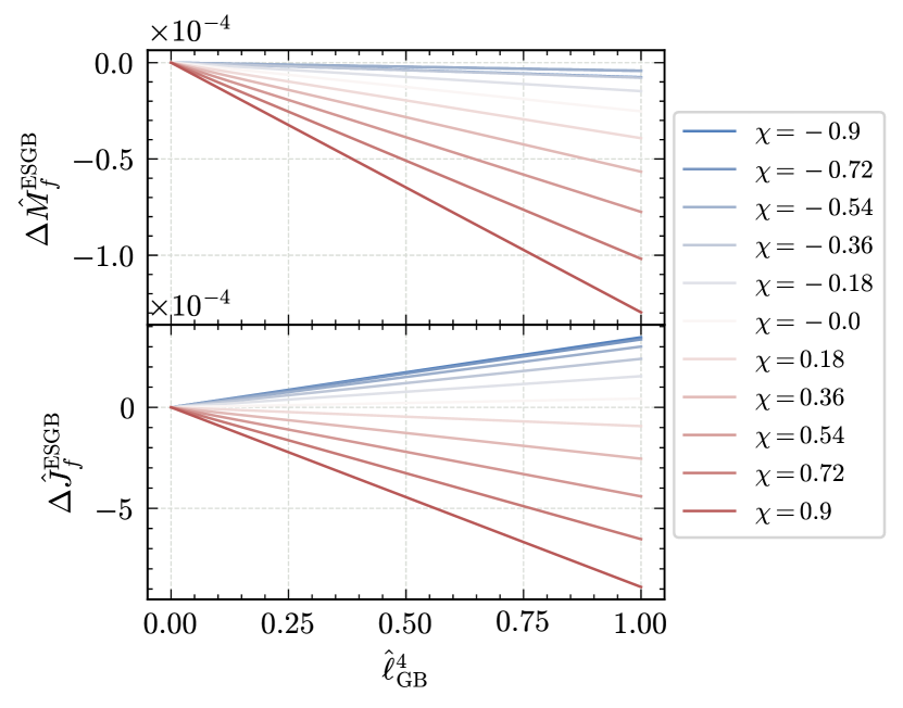
Figure 4 shows the values of the ESGB corrections to the (dimensionless) final mass and angular momentum for a set of BBHs with equal-spin magnitude and mass ratio , as a function of the ESGB coupling in the dilatonic theory (5). These corrections are quite modest compared to those affecting the inspiral dynamics, being for . We find that the corrections to the final mass are always negative, while the final angular momentum corrections can take both signs depending on the mass ratio and spins. Note that the value of at the ISCO can be larger when adding ESGB corrections to the EOB Hamiltonian [cf. Fig. 6 below].
One can also estimate the final mass and angular momentum by subtracting the energy and angular momentum radiated during the entire coalescence (including the merger-ringdown stage) from their initial values. These can in turn be obtained by integrating the energy and angular momentum fluxes, in both the metric and the scalar channels. The energy emitted through GWs depends on the final mass and spin , as they enter the computation of the merger-ringdown waveform modes used to compute the GW flux. One can then numerically solve for self-consistent values of the final mass and spin [33, 34], which minimize the difference between the values set for the remnant BH and those obtained by energy and angular-momentum balance. Using this method, we find that the corrections show a less clear dependence on intrinsic parameters, due to errors in the numerical integration and root-finding, making a parameter-space fit harder to perform. However, the median values of the corrections (across 10,000 configurations uniform in with and uniform in ) still show a clear scaling with , with the average correction being consistent with Eqs. (71).
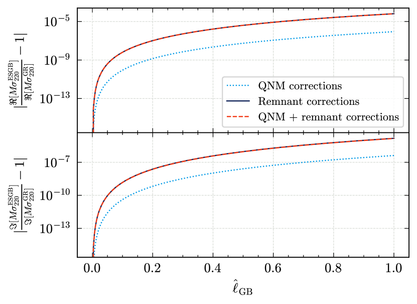
In Fig. 5, we show the fractional change between ESGB and GR in the real and imaginary part of the mode ringdown frequency, as a function of , for a nonspinning BBH (). We either include corrections to the QNM spectrum, change the final mass and spin using fits from Eq. (71), or consider both corrections. As noted in previous works [66, 40], typical corrections to the QNMs are very small. While corrections to the remnant mass and spin are also modest, they can cause changes in the frequency of the ringdown waveform from one to two orders of magnitude larger than the ESGB corrections to the QNM spectrum. The precise estimation of such corrections would be useful for high-precision tests of GR with next-generation detectors, since prospects for BH spectroscopy in ESGB could be much more optimistic than originally thought. Reference [40] found that, even with next-generation GW detectors, constraints on ESGB gravity from ringdown observations alone are weaker than current bounds from LVK inspiral observations, when only accounting for corrections to the QNM spectrum. Our results suggest that much better constraints might be achieved by exploiting complementary information from the full IMR signal.
VI Results
Given the coupling of matter fields to the metric in ESGB gravity (1), the mirrors of a GW interferometer must follow the geodesics of the perturbed Jordan metric which reads, in the Solar System:
| (73) |
where is the distance to the source, while and are the couplings of matter to the scalar field in the Solar System. Note that for the Jordan metric to reduce to Minkowski in the absence of metric and scalar waves, we must perform the local coordinate change and .
In what follows, we focus on the metric waveform , which was discussed in the previous sections. Indeed, the contribution of the scalar waveform is cut off by the numerical factor in the Solar System [234]. Moreover, we illustrate our results in the dilatonic ESGB case (5) for which , and thus and .
VI.1 Waveform morphology
In this section, we describe the impact of the ESGB corrections on the dynamics and waveforms of BBH systems, modeled with SEOBNRv5PHMESGB. As a concrete illustration, we consider a nonspinning binary with mass ratio of , and . Our conclusions remain qualitatively unchanged for different mass ratios and non-zero spins. However, in the equal-mass limit, the deviations from the GR flux are smaller, because the -1PN leading-order term in the scalar flux (IV.2) then vanishes.
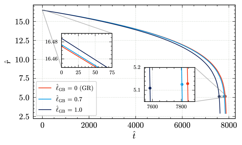
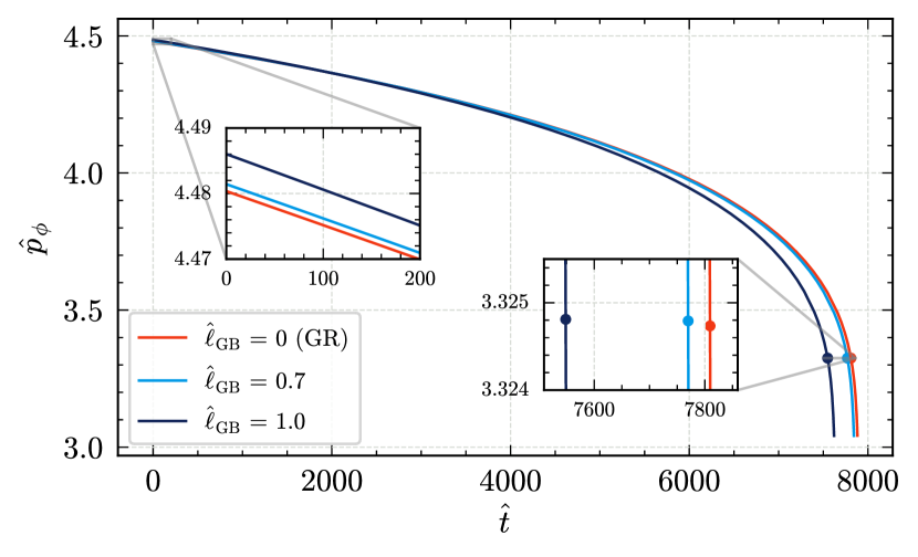
First, we examine in Fig. 6 the orbital separation and angular momentum as a function of time.
The insets highlight the differences in the dynamics at the start of the evolution, which for all cases is taken at a dimensionless orbital frequency , and close to the ISCO, indicated by the dots. The values of and at the ISCO are determined by setting both the first and second derivatives of the Hamiltonian with respect to to zero, taking (circular orbits) (i.e., ). Each curve ends at merger, taken as the peak of the (2,2) mode waveform (37). Observe that, on the examples considered:
-
1.
The binary merges at earlier times for larger values of the ESGB coupling, since more energy is radiated away due to the additional scalar field.
-
2.
Given a fixed initial dimensionless frequency, binaries start at a larger radius and angular momentum for larger values of the ESGB coupling. This is due to the replacement in the EOB potentials, with . Note that the model uses the quasi-circular, adiabatic, initial condition formulas derived in Ref. [154], also used in the SEOBNRv5PHM model.
-
3.
The ISCO is at a smaller separation [cf. also Ref. [68]] and slightly larger angular momentum compared to GR. This is a non-trivial effect due to higher-order PN corrections in the EOB Hamiltonian.
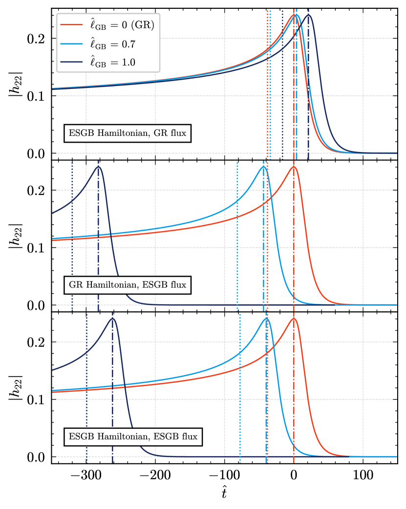
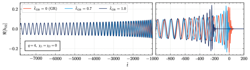
In Fig. 7 we show, for the same set of binaries, the amplitude of the (2,2) mode waveform, to highlight how a non-zero value of the coupling changes the time-to-merger when including different beyond-GR corrections. The dash-dotted vertical lines indicate the merger, taken as the peak of the (2,2) mode, and the dotted vertical lines correspond to the time at which . We set at the GR merger time. In the top panel, we incorporate ESGB corrections in the Hamiltonian, while using the GR flux, and mostly observe that modifications to the conservative dynamics tend to delay the merger. In the middle panel, we include instead ESGB corrections in the dissipative sector and use the GR Hamiltonian. As expected, these corrections accelerate the inspiral, mostly due to the additional energy dissipation via the scalar field. In the bottom panel, we combine both contributions. Changes to the dissipative dynamics are predominant, and the binary merges earlier than GR for a non-zero value of the ESGB coupling. The trend seen in this example is consistent with other cases we considered, and agrees qualitatively with NR simulations [91, 99]. Finally, Fig. 8 shows the real part of the (2,2) mode for the same set of binaries. The waveforms are aligned over a low-frequency interval, by shifting their time of coalescence and phase [cf. Sec. IV] as done in Ref. [206], and display a difference in the time-to-merger and a noticeable dephasing as they approach the merger.
Note that the ESGB corrections to the remnant mass and spin [entering the merger time and ringdown frequency, cf. Sec. V.4] and to the QNM spectrum [cf. Sec. V.3] are included in our waveforms. However, their impact is subdominant compared to the effects above.
VI.2 Quantifying measurability of deviations from GR
We now quantify which deviation magnitudes are detectable by GW detectors, and, if so, estimate the SNR required for such measurements. For this purpose, we employ a common metric in GW data analysis - the mismatch. Given two waveforms and , we introduce the overlap, defined as the noise-weighted inner product [235, 236]
| (74) |
where is the Fourier transform of the time-domain signal, and is the one-sided power spectral density (PSD) of the detector noise. The faithfulness is then defined as the overlap between the normalized waveforms, maximized over the relative time of coalescence and phase, that is
| (75) |
We finally define the mismatch, or unfaithfulness, as
| (76) |
In Eq. (74), we fix and choose different values for depending on the detector. We consider the advanced LIGO (aLIGO) detector, for which we assume the design zero-detuned high-power noise PSD [237] and , and the ET detector, for which we assume the EinsteinTelescopeP1600143 PSD implemented in pyCBC [238] and . For simplicity, we only consider the dominant (2,2) mode of the waveform when computing the mismatch.
The mismatch can be used to estimate at which SNR two signals could be distinguishable, given the detector sensitivity. This is usually formulated in terms of an indistinguishability criterion [239, 240, 241, 242], which states that if two waveforms fulfill the condition
| (77) |
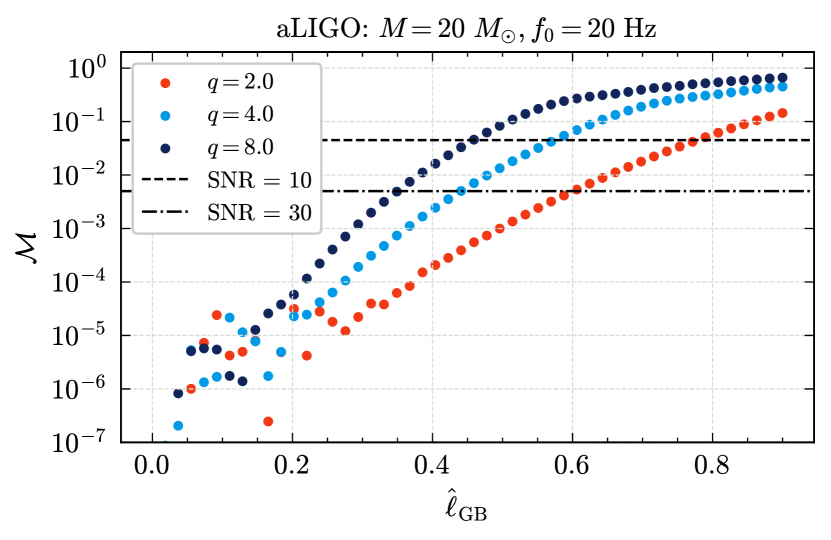
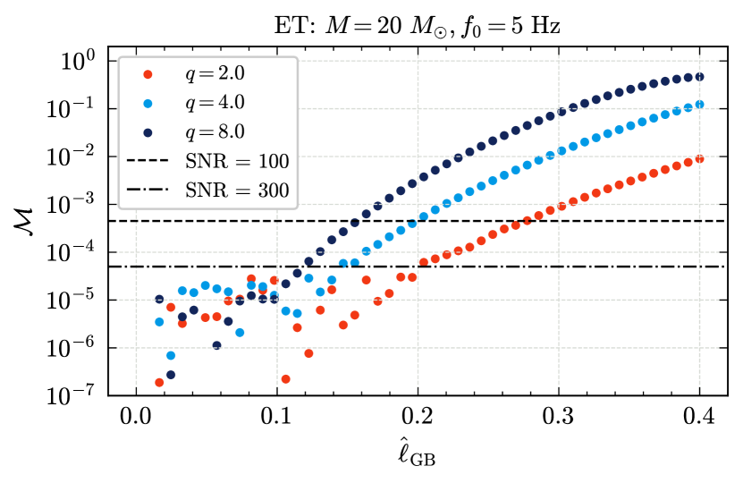
for a given PSD and SNR, then these waveforms are considered indistinguishable, and the differences in the recovered parameters are expected to be smaller than statistical errors. The prefactor can be estimated as the number of intrinsic parameters whose measure is affected by model differences [241], or it can be tuned by considering synthetic injections at increasing SNR [242]. In Fig. 9 we show the mismatch of SEOBNRv5PHMESGB against its GR limit as a function of , for the aLIGO and ET detectors. We consider a nonspinning binary with total mass and mass ratios as a signal. The horizontal lines correspond to the indistinguishability thresholds obtained by taking (our templates depend on two masses, spin components and ) for some realistic SNRs ( for aLIGO, for ET). As expected, we find a larger mismatch for more asymmetric binaries, due to the scalar dipole radiation. This results in a stronger bound on if the data is consistent with GR. The minimum value of that could be distinguished from the GR case goes from around (, ) to (, ) for aLIGO and from (, ) to (, ) for ET. The main source of improvement for ET is its larger low-frequency bandwidth, where the scalar flux dominates (see Fig. 3). Mismatch values are not to be attributed to a non-zero coupling value, as differences of this order can be simply due to errors in the numerical integration of Hamilton’s equations with finite tolerance. Comparing our results to current constraints on ESGB gravity with LVK observations, the bound on GW190814 from Refs. [168, 170] (assuming the event is from a BBH), is given as a function of the coupling with by . Taking a total mass of and a mass ratio , this corresponds to . Our prospective bound for an ET source with , translates instead to .
The potential constraints on should only be regarded as an order of magnitude estimate. Since the indistinguishability criterion offers a necessary, but not sufficient measure, if the mismatch exceeds the threshold, the differences are not necessarily measurable [243, 244]. Furthermore, only varying does not account for possible correlations between the ESGB coupling and GR parameters. For example, the main effect of a non-zero coupling being to shorten the waveform, one could expect it to be anti-correlated with the chirp mass of the binary [245],which affects the GW phase at leading PN order. Spin effects also affect the waveform in a qualitatively similar fashion, although they enter the GW phase starting from 1.5 PN order [107], and are thus expected to be less degenerate with ESGB corrections (starting from -1 PN) than the chirp mass. Therefore, this provides an optimistic estimate of the constraint derived from a single event. On the other hand, these bounds could be significantly improved by combining results from multiple observations. Since the coupling is common to all analyzed events, one can stack constraints from multiple observations by simply multiplying the marginalized likelihoods [173, 169], instead of combining the results using a hierarchical approach, assuming that beyond-GR parameters in each event are drawn from a common underlying distribution [246], as typically done for parametrized deviations.
More sophisticated predictions of the measurability of the ESGB coupling could be either based on the Fisher matrix formalism or employ full Bayesian inference. Forecasts of constraints with future detectors on ESGB gravity, as well as on other beyond-GR theories, have been obtained in Ref. [18]. This work performed a Fisher analysis including corrections to the inspiral waveform based on the parameterized post-Einsteinian (ppE) framework [21], mapping then the ppE results to theory-specific constraints, also including the effect of stacking multiple observations. A similar study, focused instead on the ringdown stage, was recently presented in Ref. [40], using the parametrized spin-expansion coefficients (ParSpec) framework [28].
Similar analyses could be refined by repeating them with SEOBNRv5PHMESGB . Ref. [18] employed as baseline GR waveform IMRPhenomPv2 [147], which is a less accurate model than SEOBNRv5PHM. It does not include higher modes and employs a simplified modeling of spin precession. It also focused on estimating modifications at a single PN order at a time, while in our model, modifications at each PN order are specified as a function of the coupling parameter of the theory. Furthermore, we include beyond-GR corrections in both the inspiral and the ringdown stages. One could employ Bayesian parameter estimation to provide forecasts for the next-generation GW detectors ET and CE, examining correlations among different parameters. We leave such analyses for future work. However, to show a practical application of SEOBNRv5PHMESGB to GW data analysis, we perform full Bayesian parameter estimation on some of the GW events reported by the LVK collaboration.
VI.3 Constraining the ESGB coupling
As an application of SEOBNRv5PHMESGB to GW data analysis, we perform full Bayesian parameter estimation for some GW events reported by the LVK collaboration, also including the ESGB coupling constant [or equivalently , cf. Footnote 2] in the analysis. We consider three signals, GW190814 [247], GW190412 [248] and GW230529 [249], which were recently analyzed in Refs. [169, 168, 170, 171, 172] to provide constraints on the coupling of the dilatonic ESGB theory (5), using waveform models featuring ESGB corrections in the inspiral phase.
We expect larger corrections to the waveform for systems with smaller masses, as the leading ESGB corrections to the phase are proportional to [61, 68, 170, 171], as well as for large mass ratios, due to the increased scalar dipole radiation [cf. Sec IV.2]. As the sources of GW190412 and GW190814 are relatively low-mass binaries with asymmetric masses, these events are expected to offer better constraints on this theory. The source of GW190814, having a secondary with a mass around , is consistent with being either a BBH or a NSBH. Under the hypothesis of GW190814 being a BBH, it imposes stringent bounds on ESGB gravity around [168, 170]. However, this bound is not necessarily robust as it changes significantly whether one assumes the event to be an NSBH or a BBH. Indeed, the scalar monopole vanishes for a NS in shift-symmetric ESGB gravity, so the correction can be much larger for a BBH than for a NSBH, whose hair is carried by the BH (which is more massive) [169, 170].
The most probable interpretation of the source of GW230529 is that of a NSBH with the primary being a BH with mass . Under this hypothesis, it currently places the best constraint on ESGB gravity [171, 172], with a bound on ranging from to depending on the waveform approximant employed, when including ESGB corrections in the inspiral phase. We note that for GW230529 one cannot determine from GW data alone if either component of the source is a NS or a BH, and the primary analysis from the LVK collaboration [249] employed BBH waveforms, including the SEOBNRv5PHM model used here as a baseline GR approximant. Furthermore, Ref. [171] finds that, when considering parameterized deviations to the inspiral phase, NSBH and BNS results with the tides constrained to realistic values are very similar to the BBH results. Therefore, in our analysis, we also neglect tidal effects, but we take the sensitivities for the secondary to be 0, as is the case for NSs in shift-symmetric ESGB theories and in the dilatonic ESGB theory at leading order in the coupling [cf. Sec II.3]. In this work we concentrate on GW190814 and GW190412 under the BBH assumption, and on GW230529 under the NSBH assumption, for simplicity.
| Event | GW230529 | GW190814 | GW190412 | Combined |
| IMR | () | () | () | () |
| IMR with merger deviations | – | () | () | () |
| Inspiral only | – | () | () | () |
The goal of Bayesian parameter estimation is to infer the posterior distribution for the parameters given the observed data , using Bayes theorem
| (78) |
where is the likelihood of the data given the parameters , is the prior on , and is the evidence. To determine whether a model is preferred over a model , one can look at the Bayes factor, defined as the ratio of the evidence for the two different models (see, e.g., Ref. [250] for a review).
We perform the analysis using parallel Bilby [251], a highly parallelized version of the Bilby [252, 253] parameter-estimation code, and the nested sampler dynesty [254] using the acceptance-walk stepping method. We use the recommended setting for the number of accepted MCMC-chains , number of live points , and set the remaining sampling parameters to their default values. For GW190814, we find that these settings were not sufficient to fully resolve the posterior distribution, and use , and . We employ strain data from the Gravitational Wave Open Source Catalog (GWOSC) [255] and the released PSD and calibration envelopes. We use the same priors for the GR parameters as those employed in Refs. [157, 249], in which these events have been analyzed using the SEOBNRv5PHM waveform model, and uniform priors on , with the constraint in the BBH case [cf. Sec. II.3]. In the NSBH case, we rather impose . To facilitate a more direct comparison with other results in the literature, we also perform inspiral-only analyses, taking a maximum frequency for the likelihood of for GW190814 and for GW190412, following Ref. [168]. These frequencies coincide with the ISCO frequency in GR, and thus, doing so amounts to cutting off the late stages of our inspiral-plunge waveforms above. We don’t perform an inspiral-only analysis for GW230529 since the cutoff frequency for the inspiral stage would be around , and while the default analysis extends up to , we don’t expect significant differences due to the reduced sensitivity of the LIGO detectors in this high-frequency range.
As detailed in Sec. V.2, our model allows for parametrized deviations in the merger waveform amplitude and frequency (69), which can be varied during sampling. We perform runs assuming that they take GR values, as well as allowing them to vary for the mode. We use uniform priors in the range for both and . We introduce additional merger parameters only in the IMR analysis, as the merger deviations do not significantly impact the results when only analyzing the inspiral. For the same reason, we don’t include these corrections in the analysis of GW230529, which has negligible SNR in the merger-ringdown stage.
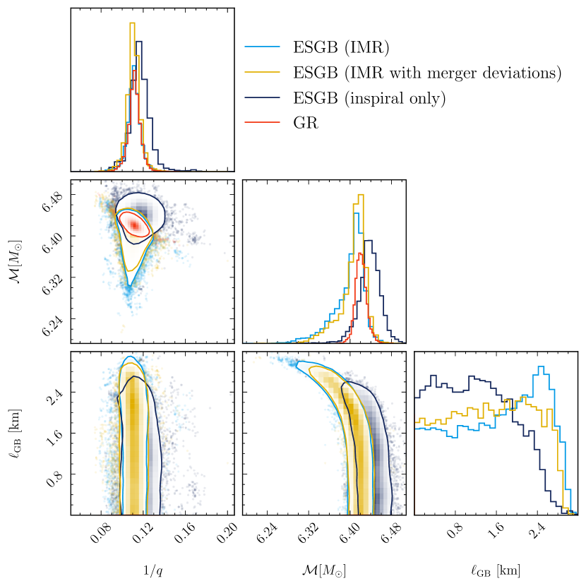
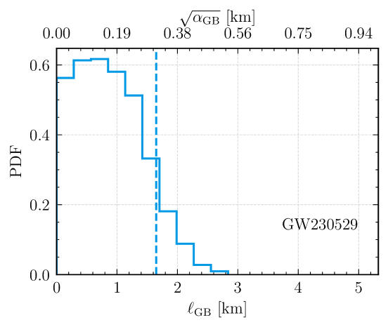
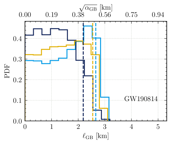
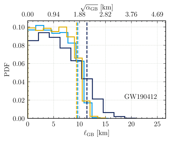
Figure 10 presents the 1-dimensional posteriors of (or, equivalently, ), marginalized over all other parameters, resulting from the analysis of GW230529, GW190814 and GW190412. The vertical dashed lines indicate the confidence bounds, also summarized in Table 3. We show the posteriors for the full IMR analyses, without adding corrections to the merger amplitude and frequency (light blue) and marginalized over parameterized merger deviations (yellow), and for inspiral-only analyses (dark blue). In all cases, the posteriors are compatible with .
For the NSBH event GW230529, we find a bound on of . Our bound is slightly less stringent than those of Refs. [171, 172] when relying on a BBH baseline model in GR, as they found and , respectively. However, our analysis differs in three ways: (i) we include ESGB corrections at higher PN orders. The references above indeed include corrections to the conservative sector at 2PN, and to the dissipative sector at 1.5PN and 1PN relatively to the quadrupolar order, respectively; (ii) our model resums these ESGB corrections within the EOB framework; (iii) the waveform models of these works are not the same as ours in the GR limit, i.e. SEOBNRv4HMROM [256] and IMRPhenomXPHM [148] respectively. This last point alone can induce comparable bound discrepancies between these works.
For GW190814, our results are also in agreement with those of Refs. [168, 170], with a bound on ranging from to . We notice that, for this event, the inspiral-only analysis provides a slightly better constraint compared to the IMR analyses. Figure 11 shows the posterior distribution of , inverse mass ratio and chirp mass inferred from GW190814, along with the mass values recovered assuming GR. We observe: (i) a slight anti-correlation between and the chirp mass, whether the plunge-merger-ringdown is included or not, as expected for inspiral-dominated signals [cf. Sec. VI.2]; and (ii) that neglecting the plunge-merger-ringdown signal results in a wider chirp mass posterior shifted towards larger values. These two points might contribute to the slightly better constraint from the inspiral-only analysis. Another factor could be that the merger-ringdown waveform is practically indistinguishable from GR for this event. Therefore, its inclusion reduces the mismatch of the waveform with its GR counterpart at fixed .
For the BBH event GW190412, we obtain a constraint from the inspiral-only analysis and a slightly tighter bound when including the plunge-merger-ringdown portions of the signal, thanks to the additional SNR. This is roughly a factor smaller compared to previous analyses [168]. The larger chirp mass of the source (, versus for GW190814 and for GW230529) results in a higher relative SNR in the late-inspiral stage, increasing the impact of higher order PN corrections and the EOB resummation. For GW190412 and GW190814, the bounds on are robust with respect to uncertainties in the merger morphology, with a slight decreas when marginalized over parameterized merger deviations.
Combining the constraints from individual events by multiplying the marginalized posteriors, we obtain a combined bound on ranging from (for the inspiral-only analyses) to (for the IMR analyses, with and without merger deviations respectively). The combined result is very similar to the one obtained by analyzing GW230529 alone, and if anything slightly worsened in the IMR analyses by the fact that the posterior for GW190814 peaks slightly away from 0.
We find, a posteriori, that our bounds are within the small-coupling limit. This justifies using the QNM expressions from Ref. [138], as well as employing the leading-order expressions (6) and (7) for the quantities in Eqs. (4) when analyzing GW230529 [cf. Sec. II.3]. For GW230529, we find at confidence. For GW190412 we obtain , while for GW190814 .
Table 4 summarizes the natural log-Bayes factors between the ESGB and GR hypotheses, inferred from the full IMR analyses of the signals. Without adding deviations to the merger amplitude and frequency, we find a log Bayes factor of for GW230529, of for GW190814 and of GW190412, indicating no substantial preference for either hypothesis [257]. When adding parametrized merger deviations, we obtain lower Bayes factors, of for GW190814 and of GW190412. This means that they do not improve how well our model fits the data, which is consistent with GW190412 and GW190814 being inspiral-dominated signals with low SNR in the merger-ringdown. The decrease in the Bayes factor is then the manifestation of the Occam penalty for introducing additional parameters. Accurate modeling of the merger phase with NR simulations in ESGB gravity would be valuable to improve this analysis.
We note that the computational cost of these runs is similar to the corresponding GR analyses with SEOBNRv5PHM, slightly higher due to additional parameters and a marginally longer waveform evaluation time. They took around 36 hours for GW190412 (256 cores), 3 days for GW190814 (384 cores) and 5 days for GW230529 (640 cores), with each analysis requiring waveform evaluations.
Our combined result could be further improved by also including the NSBH events GW200105, GW200115, which also place competitive bounds on this theory [170], as well as selected BBH events. Since the NSBHs are low-mass binaries, leading to inspiral-dominated signals, the constraints on ESGB gravity would likely be similar to those obtained by Ref. [170], which found the result to be robust with respect to the inclusion of higher-order PN corrections. On the other hand, slightly improved bounds could be obtained for heavier binaries when using SEOBNRv5PHMESGB . However, the result obtained by combining several events would likely improve only marginally, as GW230529 provides a much more stringent bound compared to other events. This is a computationally expensive but still feasible analysis that we leave for future work. Another way to improve the combined constraint we present here would be to incorporate information about the underlying astrophysical population following Ref. [258], by simultaneously inferring the astrophysical distribution to correctly account for correlations between intrinsic and beyond-GR parameters.
| Event | GW230529 | GW190814 | GW190412 |
| IMR | |||
| IMR with merger deviations | — |
VII Conclusions
Using the pySEOBNR code [167], we built the first IMR waveform model in a beyond-GR theory within the EOB approach, focusing on ESGB gravity for BBHs. The SEOBNRv5PHMESGB waveforms reduce to the SEOBNRv5PHM model [157] in the GR limit. The EOB Hamiltonian and fluxes in the pySEOBNR code can be used to build IMR waveforms for BBHs and inspiral waveforms for BNS and NSBHs in any ESGB (or ST) theory. The EOB Hamiltonian [cf. Sec. III] includes ESGB (and ST) corrections through 3PN order [68], while the metric modes in factorized form and the scalar flux entering the RR force contain ESGB (and ST) corrections through 2PN and 2.5PN (relative to the scalar dipolar) orders, respectively [cf. Sec. IV]. We recall that the factorized ESGB (and ST) metric modes [cf. Sec. V.1] are a new result of this paper. While the ESGB inspiral waveform is theory specific, the merger-ringdown waveform follows phenomenological ansätze used in GR [211, 210, 212, 156], augmented with an agnostic parameterization for the modes’ amplitude and frequency at merger, inspired by Refs. [25, 30, 166]. It also uses corrections to the QNMs frequencies and decay times derived in ESGB theory [138] and corrections to the remnant mass and spin, which we find can cause changes in the frequency of the ringdown waveform from one to two orders of magnitude larger than the ESGB corrections to the QNM spectrum. Although our model can be applied to different ESGB coupling functions, we focused our investigation to dilatonic ESGB gravity.
In Sec. VI.1, we analyzed the morphology of the dilatonic ESGB waveforms, and contrasted them with the GR ones, finding that the ESGB corrections in the conservative and dissipative dynamics cause a BBH to merge in a shorter time than in GR, when starting at the same orbital frequency (see Fig. 8). We provided measurability estimates of the ESGB coupling [cf. Sec. VI.2] based on the mismatch criterion for upcoming runs of the LVK collaboration and future ground-based detectors, such as the Einstein Telescope [cf. Fig. 9]. The bound from a single asymmetric () BBH observed with ET could be one order of magnitude better than current constraints using LVK data. Low-mass NSBHs could also be “golden” binary sources, as exemplified by GW230529. This indicates that stellar-mass binaries observed with next-generation ground-based detectors are ideal candidates to test this theory, also thanks to their high expected rates [259], and would likely provide better constraints than extreme-mass-ratio-inspirals seen with LISA [260].
We also used SEOBNRv5PHMESGB to place constraints on the coupling of the dilatonic ESGB theory using GW observations and performed Bayesian model selection between ESGB and GR [cf. Sec. VI.3]. We found that the GW events GW190412, GW190814 and GW230529 are consistent with GR, and we constrained the fundamental coupling of the theory to be () at 90 confidence. Among the events we analyzed, GW230529 provides the most stringent constraint, consistently with other recent analyses [171, 172].
It will be very beneficial to validate SEOBNRv5PHMESGB against NR simulations in ESGB gravity and to calibrate it using NR data, particularly by including NR information for the merger phase, and by guiding resummations of the PN scalar flux. Despite remarkable progress in NR evolutions of BBHs in ESGB gravity [80, 84, 85, 83, 87, 88, 91, 100, 99] and NSBH binaries [104], the number and length of current simulations, as well as their accuracy, have so far prevented us from carrying out these studies.
We limited our investigation to BHs that have already scalarized. However, ESGB gravity also allows for dynamical scalarization [135, 72]. Interesting work has been done to model dynamical scalarization [133, 134, 135, 136], and we plan to extend SEOBNRv5PHMESGB to include these nonperturbative effects, which can largely affect the waveforms toward merger, producing distinctive signatures that are absent in GR.
Furthermore, it should be straightforward to include in our waveform model ESGB corrections in the spinning sector, once they are available. Another extension of our model would involve describing complete waveforms for BNSs and NSBHs in both ST and ESGB theories, once these models have been finalized in GR within the SEOBNRv5 family.
On the data-analysis side, the simple forecast we presented for upcoming runs of the LVK collaboration and next-generation ground-based GW detectors can be extended to a broader region of the binary’s parameter space by using linear-signal approximation methods, such as the Fisher matrix formalism. Furthermore, they can be made more realistic by stacking many events and taking into account astrophysical populations [258]. Results for selected events can be validated by performing synthetic injection and analyzing them with Bayesian inference. Furthermore, our model can be used to validate results obtained with parametrized tests of GR [23, 31] and to test their effectiveness in different regions of the parameter space. It would also be interesting to analyze more LVK events, including the NSBHs GW200105, GW200115 and selected low-mass BBHs, to improve the combined constraints on . However, the results would likely only improve marginally, as GW230529 provides a much more stringent bound compared to other events.
Acknowledgments
It is a pleasure to thank Maxence Corman, Quentin Henry, Elisa Maggio, Elise Sänger, Hector Okada da Silva, and David Trestini for useful discussions. We also thank Raffi Enficiaud for his assistance with scientific computing.
The computational work for this manuscript was carried out on the Hypatia computer cluster at the Max Planck Institute for Gravitational Physics in Potsdam. This work made use of the python package pySEOBNR [167]. Stable versions of pySEOBNR are published through the Python Package Index (PyPI), and can be installed via pip install pyseobnr.
This research used data or software obtained from the Gravitational Wave Open Science Center (gwosc.org), a service of the LIGO Scientific Collaboration, the Virgo Collaboration, and KAGRA. This material is based upon work supported by NSF’s LIGO Laboratory, a major facility fully funded by the National Science Foundation, as well as the Science and Technology Facilities Council (STFC) of the United Kingdom, the Max-Planck-Society (MPS), and the State of Niedersachsen/Germany for support of the construction of Advanced LIGO and construction and operation of the GEO600 detector. Additional support for Advanced LIGO was provided by the Australian Research Council. Virgo is funded, through the European Gravitational Observatory (EGO), by the French Centre National de Recherche Scientifique (CNRS), the Italian Istituto Nazionale di Fisica Nucleare (INFN) and the Dutch Nikhef, with contributions by institutions from Belgium, Germany, Greece, Hungary, Ireland, Japan, Monaco, Poland, Portugal, Spain. KAGRA is supported by Ministry of Education, Culture, Sports, Science and Technology (MEXT), Japan Society for the Promotion of Science (JSPS) in Japan; National Research Foundation (NRF) and Ministry of Science and ICT (MSIT) in Korea; Academia Sinica (AS) and National Science and Technology Council (NSTC) in Taiwan.
Appendix A Einstein and Jordan frames
In Refs. [47, 57, 58], the ST two-body Lagrangian was derived up to 3PN order by adopting the Jordan-frame formulation of the theory:
| (79) |
using tildes for clarity. Here, , and is a function defining the theory. As for compact bodies, they were described by the point particle action
| (80) |
with . By contrast, we adopt here the Einstein-frame formulation of ST theories:
| (81) |
where , and we account for compact bodies by the substitution
| (82) |
with . The actions (79)-(80) and (81)-(82) are the same, modulo boundary terms and the following redefinitions:
| (83a) | ||||
| (83b) | ||||
| (83c) | ||||
where is obtained by inverting . We also introduce the notation:
| (84a) | ||||
| (84b) | ||||
| (84c) | ||||
| (84d) | ||||
where the subscript denotes a quantity evaluated at infinity, . The quantities above can be obtained by inserting Eq. (83c) into Eqs. (4) and taking the limit , in which case body is said to have negligible self-gravity.
Appendix B ESGB corrections to the EOB potentials
The coefficients , and entering Eqs. (14) were calculated in Refs. [52, 68]. They read:
| (85a) | ||||
| (85b) | ||||
| (85c) | ||||
| (86a) | ||||
and, finally,
| (87a) | ||||
| (87b) | ||||
Appendix C Factors of the metric modes
Here, we give the explicit factors that are nonzero at 2PN, with . Note that originates from memory effects [51]. It does not contribute to the metric flux on circular orbits (20) because , but it enters the metric waveform.
| (88a) | ||||
| (88b) | ||||
| (88c) | ||||
| (88d) | ||||
| (88e) | ||||
| (88f) | ||||
| (88g) | ||||
| (88h) | ||||
| (88i) | ||||
| (88j) | ||||
| (88k) | ||||
| (88l) | ||||
| (88m) | ||||
| (88n) | ||||
| (88o) | ||||
| (88p) | ||||
| (88q) | ||||
| (88r) | ||||
Appendix D Coefficients of the scalar flux
The coefficients entering the scalar flux (IV.2) read:
| (89a) | ||||
| (89b) | ||||
| (89c) | ||||
| (89d) | ||||
| (89e) | ||||
Appendix E Decomposition of the scalar waveform on spherical harmonics
The scalar waveform (33) can be decomposed in a similar fashion as its metric counterpart over spherical harmonics (of weight zero),
| (90) |
where the modes were calculated in Ref. [64] at 1.5PN relative to the dipolar order. We translate them following the steps detailed in Sec. IV.2 . In the radiative coordinate system (27), we find:
| (91) |
where and were defined in Eqs. (29) and (30), respectively. The nonzero, dimensionless factors then read, for :
| (92a) | ||||
| (92b) | ||||
| (92c) | ||||
| (92d) | ||||
| (92e) | ||||
| (92f) | ||||
| (92g) | ||||
The monopolar contribution does not contribute to the scalar flux (34) on circular orbits, because . Thus, the scalar flux is dominated by the dipolar mode . Note that the orbit being planar, we have by symmetry [196]
| (93) |
References
- [1] LIGO Scientific, Virgo collaboration, B. P. Abbott et al., Observation of Gravitational Waves from a Binary Black Hole Merger, Phys. Rev. Lett. 116 (2016) 061102 [1602.03837].
- [2] LIGO Scientific, Virgo collaboration, B. P. Abbott et al., GWTC-1: A Gravitational-Wave Transient Catalog of Compact Binary Mergers Observed by LIGO and Virgo during the First and Second Observing Runs, Phys. Rev. X 9 (2019) 031040 [1811.12907].
- [3] LIGO Scientific, VIRGO collaboration, R. Abbott et al., GWTC-2.1: Deep Extended Catalog of Compact Binary Coalescences Observed by LIGO and Virgo During the First Half of the Third Observing Run, 2108.01045.
- [4] KAGRA, VIRGO, LIGO Scientific collaboration, R. Abbott et al., GWTC-3: Compact Binary Coalescences Observed by LIGO and Virgo during the Second Part of the Third Observing Run, Phys. Rev. X 13 (2023) 041039 [2111.03606].
- [5] A. H. Nitz, S. Kumar, Y.-F. Wang, S. Kastha, S. Wu, M. Schäfer et al., 4-OGC: Catalog of Gravitational Waves from Compact Binary Mergers, Astrophys. J. 946 (2023) 59 [2112.06878].
- [6] A. K. Mehta, S. Olsen, D. Wadekar, J. Roulet, T. Venumadhav, J. Mushkin et al., New binary black hole mergers in the LIGO-Virgo O3b data, 2311.06061.
- [7] LIGO Scientific collaboration, J. Aasi et al., Advanced LIGO, Class. Quant. Grav. 32 (2015) 074001 [1411.4547].
- [8] VIRGO collaboration, F. Acernese et al., Advanced Virgo: a second-generation interferometric gravitational wave detector, Class. Quant. Grav. 32 (2015) 024001 [1408.3978].
- [9] LIGO Scientific, Virgo collaboration, B. P. Abbott et al., Tests of general relativity with GW150914, Phys. Rev. Lett. 116 (2016) 221101 [1602.03841].
- [10] LIGO Scientific, Virgo collaboration, B. P. Abbott et al., Tests of General Relativity with GW170817, Phys. Rev. Lett. 123 (2019) 011102 [1811.00364].
- [11] LIGO Scientific, Virgo collaboration, B. P. Abbott et al., Tests of General Relativity with the Binary Black Hole Signals from the LIGO-Virgo Catalog GWTC-1, Phys. Rev. D 100 (2019) 104036 [1903.04467].
- [12] LIGO Scientific, Virgo collaboration, R. Abbott et al., Tests of general relativity with binary black holes from the second LIGO-Virgo gravitational-wave transient catalog, Phys. Rev. D 103 (2021) 122002 [2010.14529].
- [13] LIGO Scientific, VIRGO, KAGRA collaboration, R. Abbott et al., Tests of General Relativity with GWTC-3, 2112.06861.
- [14] KAGRA collaboration, T. Akutsu et al., Overview of KAGRA: Detector design and construction history, PTEP 2021 (2021) 05A101 [2005.05574].
- [15] M. Punturo et al., The Einstein Telescope: A third-generation gravitational wave observatory, Class. Quant. Grav. 27 (2010) 194002.
- [16] M. Evans et al., A Horizon Study for Cosmic Explorer: Science, Observatories, and Community, 2109.09882.
- [17] LISA collaboration, P. Amaro-Seoane et al., Laser Interferometer Space Antenna, 1702.00786.
- [18] S. E. Perkins, N. Yunes and E. Berti, Probing Fundamental Physics with Gravitational Waves: The Next Generation, Phys. Rev. D 103 (2021) 044024 [2010.09010].
- [19] L. Blanchet and B. S. Sathyaprakash, Detecting the tail effect in gravitational wave experiments, Phys. Rev. Lett. 74 (1995) 1067.
- [20] K. G. Arun, B. R. Iyer, M. S. S. Qusailah and B. S. Sathyaprakash, Probing the non-linear structure of general relativity with black hole binaries, Phys. Rev. D 74 (2006) 024006 [gr-qc/0604067].
- [21] N. Yunes and F. Pretorius, Fundamental Theoretical Bias in Gravitational Wave Astrophysics and the Parameterized Post-Einsteinian Framework, Phys. Rev. D 80 (2009) 122003 [0909.3328].
- [22] T. G. F. Li, W. Del Pozzo, S. Vitale, C. Van Den Broeck, M. Agathos, J. Veitch et al., Towards a generic test of the strong field dynamics of general relativity using compact binary coalescence, Phys. Rev. D 85 (2012) 082003 [1110.0530].
- [23] M. Agathos, W. Del Pozzo, T. G. F. Li, C. Van Den Broeck, J. Veitch and S. Vitale, TIGER: A data analysis pipeline for testing the strong-field dynamics of general relativity with gravitational wave signals from coalescing compact binaries, Phys. Rev. D 89 (2014) 082001 [1311.0420].
- [24] E. Barausse, N. Yunes and K. Chamberlain, Theory-Agnostic Constraints on Black-Hole Dipole Radiation with Multiband Gravitational-Wave Astrophysics, Phys. Rev. Lett. 116 (2016) 241104 [1603.04075].
- [25] R. Brito, A. Buonanno and V. Raymond, Black-hole Spectroscopy by Making Full Use of Gravitational-Wave Modeling, Phys. Rev. D 98 (2018) 084038 [1805.00293].
- [26] V. Cardoso, M. Kimura, A. Maselli, E. Berti, C. F. B. Macedo and R. McManus, Parametrized black hole quasinormal ringdown: Decoupled equations for nonrotating black holes, Phys. Rev. D 99 (2019) 104077 [1901.01265].
- [27] R. McManus, E. Berti, C. F. B. Macedo, M. Kimura, A. Maselli and V. Cardoso, Parametrized black hole quasinormal ringdown. II. Coupled equations and quadratic corrections for nonrotating black holes, Phys. Rev. D 100 (2019) 044061 [1906.05155].
- [28] A. Maselli, P. Pani, L. Gualtieri and E. Berti, Parametrized ringdown spin expansion coefficients: a data-analysis framework for black-hole spectroscopy with multiple events, Phys. Rev. D 101 (2020) 024043 [1910.12893].
- [29] G. Carullo, W. Del Pozzo and J. Veitch, Observational Black Hole Spectroscopy: A time-domain multimode analysis of GW150914, Phys. Rev. D 99 (2019) 123029 [1902.07527].
- [30] A. Ghosh, R. Brito and A. Buonanno, Constraints on quasinormal-mode frequencies with LIGO-Virgo binary–black-hole observations, Phys. Rev. D 103 (2021) 124041 [2104.01906].
- [31] A. K. Mehta, A. Buonanno, R. Cotesta, A. Ghosh, N. Sennett and J. Steinhoff, Tests of general relativity with gravitational-wave observations using a flexible theory-independent method, Phys. Rev. D 107 (2023) 044020 [2203.13937].
- [32] S. A. Hughes and K. Menou, Golden binaries for LISA: Robust probes of strong-field gravity, Astrophys. J. 623 (2005) 689 [astro-ph/0410148].
- [33] A. Ghosh et al., Testing general relativity using golden black-hole binaries, Phys. Rev. D 94 (2016) 021101 [1602.02453].
- [34] A. Ghosh, N. K. Johnson-Mcdaniel, A. Ghosh, C. K. Mishra, P. Ajith, W. Del Pozzo et al., Testing general relativity using gravitational wave signals from the inspiral, merger and ringdown of binary black holes, Class. Quant. Grav. 35 (2018) 014002 [1704.06784].
- [35] S. S. Madekar, N. K. Johnson-McDaniel, A. Gupta and A. Ghosh, A meta inspiral-merger-ringdown consistency test of general relativity with gravitational wave signals from compact binaries, 2405.05884.
- [36] C. M. Will, The Confrontation between General Relativity and Experiment, Living Rev. Rel. 17 (2014) 4 [1403.7377].
- [37] E. Berti et al., Testing General Relativity with Present and Future Astrophysical Observations, Class. Quant. Grav. 32 (2015) 243001 [1501.07274].
- [38] N. Yunes, K. Yagi and F. Pretorius, Theoretical Physics Implications of the Binary Black-Hole Mergers GW150914 and GW151226, Phys. Rev. D 94 (2016) 084002 [1603.08955].
- [39] H. O. Silva, A. Ghosh and A. Buonanno, Black-hole ringdown as a probe of higher-curvature gravity theories, Phys. Rev. D 107 (2023) 044030 [2205.05132].
- [40] A. Maselli, S. Yi, L. Pierini, V. Vellucci, L. Reali, L. Gualtieri et al., Black hole spectroscopy beyond Kerr: agnostic and theory-based tests with next-generation interferometers, 2311.14803.
- [41] S. Datta, M. Saleem, K. G. Arun and B. S. Sathyaprakash, Multiparameter tests of general relativity using principal component analysis with next-generation gravitational wave detectors, 2208.07757.
- [42] Y. Xie, D. Chatterjee, G. Narayan and N. Yunes, Neural Post-Einsteinian Framework for Efficient Theory-Agnostic Tests of General Relativity with Gravitational Waves, 2403.18936.
- [43] T. Damour and G. Esposito-Farese, Tensor multiscalar theories of gravitation, Class. Quant. Grav. 9 (1992) 2093.
- [44] T. Damour and G. Esposito-Farese, Nonperturbative strong field effects in tensor - scalar theories of gravitation, Phys. Rev. Lett. 70 (1993) 2220.
- [45] P. Pani and V. Cardoso, Are black holes in alternative theories serious astrophysical candidates? The Case for Einstein-Dilaton-Gauss-Bonnet black holes, Phys. Rev. D 79 (2009) 084031 [0902.1569].
- [46] K. Yagi, L. C. Stein, N. Yunes and T. Tanaka, Post-Newtonian, Quasi-Circular Binary Inspirals in Quadratic Modified Gravity, Phys. Rev. D 85 (2012) 064022 [1110.5950].
- [47] S. Mirshekari and C. M. Will, Compact binary systems in scalar-tensor gravity: Equations of motion to 2.5 post-Newtonian order, Phys. Rev. D 87 (2013) 084070 [1301.4680].
- [48] R. N. Lang, Compact binary systems in scalar-tensor gravity. II. Tensor gravitational waves to second post-Newtonian order, Phys. Rev. D 89 (2014) 084014 [1310.3320].
- [49] R. N. Lang, Compact binary systems in scalar-tensor gravity. III. Scalar waves and energy flux, Phys. Rev. D 91 (2015) 084027 [1411.3073].
- [50] J. L. Blázquez-Salcedo, C. F. B. Macedo, V. Cardoso, V. Ferrari, L. Gualtieri, F. S. Khoo et al., Perturbed black holes in Einstein-dilaton-Gauss-Bonnet gravity: Stability, ringdown, and gravitational-wave emission, Phys. Rev. D 94 (2016) 104024 [1609.01286].
- [51] N. Sennett, S. Marsat and A. Buonanno, Gravitational waveforms in scalar-tensor gravity at 2PN relative order, Phys. Rev. D 94 (2016) 084003 [1607.01420].
- [52] F.-L. Julié and N. Deruelle, Two-body problem in Scalar-Tensor theories as a deformation of General Relativity : an Effective-One-Body approach, Phys. Rev. D 95 (2017) 124054 [1703.05360].
- [53] F.-L. Julié, Reducing the two-body problem in scalar-tensor theories to the motion of a test particle : a scalar-tensor effective-one-body approach, Phys. Rev. D 97 (2018) 024047 [1709.09742].
- [54] F.-L. Julié, On the motion of hairy black holes in Einstein-Maxwell-dilaton theories, JCAP 01 (2018) 026 [1711.10769].
- [55] M. Cárdenas, F.-L. Julié and N. Deruelle, Thermodynamics sheds light on black hole dynamics, Phys. Rev. D 97 (2018) 124021 [1712.02672].
- [56] F.-L. Julié, Gravitational radiation from compact binary systems in Einstein-Maxwell-dilaton theories, JCAP 10 (2018) 033 [1809.05041].
- [57] L. Bernard, Dynamics of compact binary systems in scalar-tensor theories: Equations of motion to the third post-Newtonian order, Phys. Rev. D 98 (2018) 044004 [1802.10201].
- [58] L. Bernard, Dynamics of compact binary systems in scalar-tensor theories: II. Center-of-mass and conserved quantities to 3PN order, Phys. Rev. D 99 (2019) 044047 [1812.04169].
- [59] L. Bernard, Dipolar tidal effects in scalar-tensor theories, Phys. Rev. D 101 (2020) 021501 [1906.10735].
- [60] M. Khalil, N. Sennett, J. Steinhoff, J. Vines and A. Buonanno, Hairy binary black holes in Einstein-Maxwell-dilaton theory and their effective-one-body description, Phys. Rev. D 98 (2018) 104010 [1809.03109].
- [61] F.-L. Julié and E. Berti, Post-Newtonian dynamics and black hole thermodynamics in Einstein-scalar-Gauss-Bonnet gravity, Phys. Rev. D 100 (2019) 104061 [1909.05258].
- [62] B. Shiralilou, T. Hinderer, S. M. Nissanke, N. Ortiz and H. Witek, Post-Newtonian gravitational and scalar waves in scalar-Gauss–Bonnet gravity, Class. Quant. Grav. 39 (2022) 035002 [2105.13972].
- [63] L. Pierini and L. Gualtieri, Quasi-normal modes of rotating black holes in Einstein-dilaton Gauss-Bonnet gravity: the first order in rotation, Phys. Rev. D 103 (2021) 124017 [2103.09870].
- [64] L. Bernard, L. Blanchet and D. Trestini, Gravitational waves in scalar-tensor theory to one-and-a-half post-Newtonian order, JCAP 08 (2022) 008 [2201.10924].
- [65] F.-L. Julié, H. O. Silva, E. Berti and N. Yunes, Black hole sensitivities in Einstein-scalar-Gauss-Bonnet gravity, Phys. Rev. D 105 (2022) 124031 [2202.01329].
- [66] L. Pierini and L. Gualtieri, Quasinormal modes of rotating black holes in Einstein-dilaton Gauss-Bonnet gravity: The second order in rotation, Phys. Rev. D 106 (2022) 104009 [2207.11267].
- [67] T. Jain, P. Rettegno, M. Agathos, A. Nagar and L. Turco, Effective-one-body Hamiltonian in scalar-tensor gravity at third post-Newtonian order, Phys. Rev. D 107 (2023) 084017 [2211.15580].
- [68] F.-L. Julié, V. Baibhav, E. Berti and A. Buonanno, Third post-Newtonian effective-one-body Hamiltonian in scalar-tensor and Einstein-scalar-Gauss-Bonnet gravity, Phys. Rev. D 107 (2023) 104044 [2212.13802].
- [69] T. Jain, Nonlocal-in-time effective one body Hamiltonian in scalar-tensor gravity at third post-Newtonian order, Phys. Rev. D 107 (2023) 084018 [2301.01070].
- [70] G. Creci, T. Hinderer and J. Steinhoff, Tidal properties of neutron stars in scalar-tensor theories of gravity, Phys. Rev. D 108 (2023) 124073 [2308.11323].
- [71] L. Bernard, E. Dones and S. Mougiakakos, Tidal effects up to next-to-next-to-leading post-Newtonian order in massless scalar-tensor theories, Phys. Rev. D 109 (2024) 044006 [2310.19679].
- [72] F.-L. Julié, Dynamical scalarization in Schwarzschild binary inspirals, 2312.16764.
- [73] J. Healy, T. Bode, R. Haas, E. Pazos, P. Laguna, D. Shoemaker et al., Late Inspiral and Merger of Binary Black Holes in Scalar-Tensor Theories of Gravity, Class. Quant. Grav. 29 (2012) 232002 [1112.3928].
- [74] E. Barausse, C. Palenzuela, M. Ponce and L. Lehner, Neutron-star mergers in scalar-tensor theories of gravity, Phys. Rev. D 87 (2013) 081506 [1212.5053].
- [75] E. Berti, V. Cardoso, L. Gualtieri, M. Horbatsch and U. Sperhake, Numerical simulations of single and binary black holes in scalar-tensor theories: circumventing the no-hair theorem, Phys. Rev. D 87 (2013) 124020 [1304.2836].
- [76] M. Shibata, K. Taniguchi, H. Okawa and A. Buonanno, Coalescence of binary neutron stars in a scalar-tensor theory of gravity, Phys. Rev. D 89 (2014) 084005 [1310.0627].
- [77] C. Palenzuela, E. Barausse, M. Ponce and L. Lehner, Dynamical scalarization of neutron stars in scalar-tensor gravity theories, Phys. Rev. D 89 (2014) 044024 [1310.4481].
- [78] M. Okounkova, L. C. Stein, M. A. Scheel and D. A. Hemberger, Numerical binary black hole mergers in dynamical Chern-Simons gravity: Scalar field, Phys. Rev. D 96 (2017) 044020 [1705.07924].
- [79] J. Cayuso, N. Ortiz and L. Lehner, Fixing extensions to general relativity in the nonlinear regime, Phys. Rev. D 96 (2017) 084043 [1706.07421].
- [80] H. Witek, L. Gualtieri, P. Pani and T. P. Sotiriou, Black holes and binary mergers in scalar Gauss-Bonnet gravity: scalar field dynamics, Phys. Rev. D 99 (2019) 064035 [1810.05177].
- [81] M. Okounkova, L. C. Stein, M. A. Scheel and S. A. Teukolsky, Numerical binary black hole collisions in dynamical Chern-Simons gravity, Phys. Rev. D 100 (2019) 104026 [1906.08789].
- [82] M. Okounkova, L. C. Stein, J. Moxon, M. A. Scheel and S. A. Teukolsky, Numerical relativity simulation of GW150914 beyond general relativity, Phys. Rev. D 101 (2020) 104016 [1911.02588].
- [83] M. Okounkova, Numerical relativity simulation of GW150914 in Einstein dilaton Gauss-Bonnet gravity, Phys. Rev. D 102 (2020) 084046 [2001.03571].
- [84] F.-L. Julié and E. Berti, formalism in Einstein-scalar-Gauss-Bonnet gravity, Phys. Rev. D 101 (2020) 124045 [2004.00003].
- [85] H. Witek, L. Gualtieri and P. Pani, Towards numerical relativity in scalar Gauss-Bonnet gravity: decomposition beyond the small-coupling limit, Phys. Rev. D 101 (2020) 124055 [2004.00009].
- [86] H. O. Silva, H. Witek, M. Elley and N. Yunes, Dynamical Descalarization in Binary Black Hole Mergers, Phys. Rev. Lett. 127 (2021) 031101 [2012.10436].
- [87] W. E. East and J. L. Ripley, Evolution of Einstein-scalar-Gauss-Bonnet gravity using a modified harmonic formulation, Phys. Rev. D 103 (2021) 044040 [2011.03547].
- [88] W. E. East and J. L. Ripley, Dynamics of Spontaneous Black Hole Scalarization and Mergers in Einstein-Scalar-Gauss-Bonnet Gravity, Phys. Rev. Lett. 127 (2021) 101102 [2105.08571].
- [89] P. Figueras and T. França, Black hole binaries in cubic Horndeski theories, Phys. Rev. D 105 (2022) 124004 [2112.15529].
- [90] G. Lara, M. Bezares and E. Barausse, UV completions, fixing the equations, and nonlinearities in k-essence, Phys. Rev. D 105 (2022) 064058 [2112.09186].
- [91] M. Corman, J. L. Ripley and W. E. East, Nonlinear studies of binary black hole mergers in Einstein-scalar-Gauss-Bonnet gravity, Phys. Rev. D 107 (2023) 024014 [2210.09235].
- [92] L. Aresté Saló, K. Clough and P. Figueras, Well-Posedness of the Four-Derivative Scalar-Tensor Theory of Gravity in Singularity Avoiding Coordinates, Phys. Rev. Lett. 129 (2022) 261104 [2208.14470].
- [93] D. D. Doneva, A. Vañó Viñuales and S. S. Yazadjiev, Dynamical descalarization with a jump during a black hole merger, Phys. Rev. D 106 (2022) L061502 [2204.05333].
- [94] M. Elley, H. O. Silva, H. Witek and N. Yunes, Spin-induced dynamical scalarization, descalarization, and stealthness in scalar-Gauss-Bonnet gravity during a black hole coalescence, Phys. Rev. D 106 (2022) 044018 [2205.06240].
- [95] N. Franchini, M. Bezares, E. Barausse and L. Lehner, Fixing the dynamical evolution in scalar-Gauss-Bonnet gravity, Phys. Rev. D 106 (2022) 064061 [2206.00014].
- [96] A. H. K. R, J. L. Ripley and N. Yunes, Where and why does Einstein-scalar-Gauss-Bonnet theory break down?, Phys. Rev. D 107 (2023) 044044 [2211.08477].
- [97] S. Ma, V. Varma, L. C. Stein, F. Foucart, M. D. Duez, L. E. Kidder et al., Numerical simulations of black hole-neutron star mergers in scalar-tensor gravity, Phys. Rev. D 107 (2023) 124051 [2304.11836].
- [98] R. Cayuso, P. Figueras, T. França and L. Lehner, Self-Consistent Modeling of Gravitational Theories beyond General Relativity, Phys. Rev. Lett. 131 (2023) 111403.
- [99] L. Aresté Saló, K. Clough and P. Figueras, Puncture gauge formulation for Einstein-Gauss-Bonnet gravity and four-derivative scalar-tensor theories in d+1 spacetime dimensions, Phys. Rev. D 108 (2023) 084018 [2306.14966].
- [100] D. D. Doneva, L. Aresté Saló, K. Clough, P. Figueras and S. S. Yazadjiev, Testing the limits of scalar-Gauss-Bonnet gravity through nonlinear evolutions of spin-induced scalarization, Phys. Rev. D 108 (2023) 084017 [2307.06474].
- [101] S. E. Brady, L. Aresté Saló, K. Clough, P. Figueras and A. P. S., Solving the initial conditions problem for modified gravity theories, Phys. Rev. D 108 (2023) 104022 [2308.16791].
- [102] G. Lara, H. P. Pfeiffer, N. A. Wittek, N. L. Vu, K. C. Nelli, A. Carpenter et al., Scalarization of isolated black holes in scalar Gauss-Bonnet theory in the fixing-the-equations approach, 2403.08705.
- [103] M. Corman, L. Lehner, W. E. East and G. Dideron, Nonlinear studies of modifications to general relativity: Comparing different approaches, 2405.15581.
- [104] M. Corman and W. E. East, Black hole-neutron star mergers in Einstein-scalar-Gauss-Bonnet gravity, 2405.18496.
- [105] P. J. Nee, G. Lara, H. P. Pfeiffer and N. L. Vu, Quasistationary hair for binary black hole initial data in scalar Gauss-Bonnet gravity, 2406.08410.
- [106] G. Schäfer and P. Jaranowski, Hamiltonian formulation of general relativity and post-Newtonian dynamics of compact binaries, Living Rev. Rel. 21 (2018) 7 [1805.07240].
- [107] L. Blanchet, Gravitational Radiation from Post-Newtonian Sources and Inspiralling Compact Binaries, Living Rev. Rel. 17 (2014) 2 [1310.1528].
- [108] A. Buonanno and T. Damour, Effective one-body approach to general relativistic two-body dynamics, Phys. Rev. D 59 (1999) 084006 [gr-qc/9811091].
- [109] L. Barack and A. Pound, Self-force and radiation reaction in general relativity, Rept. Prog. Phys. 82 (2019) 016904 [1805.10385].
- [110] F. Pretorius, Evolution of binary black hole spacetimes, Phys. Rev. Lett. 95 (2005) 121101 [gr-qc/0507014].
- [111] M. Campanelli, C. O. Lousto, P. Marronetti and Y. Zlochower, Accurate evolutions of orbiting black-hole binaries without excision, Phys. Rev. Lett. 96 (2006) 111101 [gr-qc/0511048].
- [112] J. G. Baker, J. Centrella, D.-I. Choi, M. Koppitz and J. van Meter, Gravitational wave extraction from an inspiraling configuration of merging black holes, Phys. Rev. Lett. 96 (2006) 111102 [gr-qc/0511103].
- [113] S. Mignemi and N. R. Stewart, Charged black holes in effective string theory, Phys. Rev. D 47 (1993) 5259 [hep-th/9212146].
- [114] T. Torii, H. Yajima and K.-i. Maeda, Dilatonic black holes with Gauss-Bonnet term, Phys. Rev. D 55 (1997) 739 [gr-qc/9606034].
- [115] N. Yunes and L. C. Stein, Non-Spinning Black Holes in Alternative Theories of Gravity, Phys. Rev. D 83 (2011) 104002 [1101.2921].
- [116] T. P. Sotiriou and S.-Y. Zhou, Black hole hair in generalized scalar-tensor gravity, Phys. Rev. Lett. 112 (2014) 251102 [1312.3622].
- [117] T. P. Sotiriou and S.-Y. Zhou, Black hole hair in generalized scalar-tensor gravity: An explicit example, Phys. Rev. D 90 (2014) 124063 [1408.1698].
- [118] P. Kanti, N. E. Mavromatos, J. Rizos, K. Tamvakis and E. Winstanley, Dilatonic black holes in higher curvature string gravity, Phys. Rev. D 54 (1996) 5049 [hep-th/9511071].
- [119] P. Pani, C. F. B. Macedo, L. C. B. Crispino and V. Cardoso, Slowly rotating black holes in alternative theories of gravity, Phys. Rev. D 84 (2011) 087501 [1109.3996].
- [120] D. Ayzenberg and N. Yunes, Slowly-Rotating Black Holes in Einstein-Dilaton-Gauss-Bonnet Gravity: Quadratic Order in Spin Solutions, Phys. Rev. D 90 (2014) 044066 [1405.2133].
- [121] A. Maselli, P. Pani, L. Gualtieri and V. Ferrari, Rotating black holes in Einstein-Dilaton-Gauss-Bonnet gravity with finite coupling, Phys. Rev. D 92 (2015) 083014 [1507.00680].
- [122] B. Kleihaus, J. Kunz, S. Mojica and E. Radu, Spinning black holes in Einstein–Gauss-Bonnet–dilaton theory: Nonperturbative solutions, Phys. Rev. D 93 (2016) 044047 [1511.05513].
- [123] G. Antoniou, A. Bakopoulos and P. Kanti, Evasion of No-Hair Theorems and Novel Black-Hole Solutions in Gauss-Bonnet Theories, Phys. Rev. Lett. 120 (2018) 131102 [1711.03390].
- [124] P. V. P. Cunha, C. A. R. Herdeiro and E. Radu, Spontaneously Scalarized Kerr Black Holes in Extended Scalar-Tensor–Gauss-Bonnet Gravity, Phys. Rev. Lett. 123 (2019) 011101 [1904.09997].
- [125] D. D. Doneva and S. S. Yazadjiev, New Gauss-Bonnet Black Holes with Curvature-Induced Scalarization in Extended Scalar-Tensor Theories, Phys. Rev. Lett. 120 (2018) 131103 [1711.01187].
- [126] H. O. Silva, J. Sakstein, L. Gualtieri, T. P. Sotiriou and E. Berti, Spontaneous scalarization of black holes and compact stars from a Gauss-Bonnet coupling, Phys. Rev. Lett. 120 (2018) 131104 [1711.02080].
- [127] M. Minamitsuji and T. Ikeda, Scalarized black holes in the presence of the coupling to Gauss-Bonnet gravity, Phys. Rev. D 99 (2019) 044017 [1812.03551].
- [128] H. O. Silva, C. F. B. Macedo, T. P. Sotiriou, L. Gualtieri, J. Sakstein and E. Berti, Stability of scalarized black hole solutions in scalar-Gauss-Bonnet gravity, Phys. Rev. D 99 (2019) 064011 [1812.05590].
- [129] C. F. B. Macedo, J. Sakstein, E. Berti, L. Gualtieri, H. O. Silva and T. P. Sotiriou, Self-interactions and Spontaneous Black Hole Scalarization, Phys. Rev. D 99 (2019) 104041 [1903.06784].
- [130] M. Minamitsuji and T. Ikeda, Spontaneous scalarization of black holes in the Horndeski theory, Phys. Rev. D 99 (2019) 104069 [1904.06572].
- [131] A. Dima, E. Barausse, N. Franchini and T. P. Sotiriou, Spin-induced black hole spontaneous scalarization, Phys. Rev. Lett. 125 (2020) 231101 [2006.03095].
- [132] D. D. Doneva, F. M. Ramazanoğlu, H. O. Silva, T. P. Sotiriou and S. S. Yazadjiev, Spontaneous scalarization, Rev. Mod. Phys. 96 (2024) 015004 [2211.01766].
- [133] N. Sennett and A. Buonanno, Modeling dynamical scalarization with a resummed post-Newtonian expansion, Phys. Rev. D 93 (2016) 124004 [1603.03300].
- [134] N. Sennett, L. Shao and J. Steinhoff, Effective action model of dynamically scalarizing binary neutron stars, Phys. Rev. D 96 (2017) 084019 [1708.08285].
- [135] M. Khalil, N. Sennett, J. Steinhoff and A. Buonanno, Theory-agnostic framework for dynamical scalarization of compact binaries, Phys. Rev. D 100 (2019) 124013 [1906.08161].
- [136] M. Khalil, R. F. P. Mendes, N. Ortiz and J. Steinhoff, Effective-action model for dynamical scalarization beyond the adiabatic approximation, Phys. Rev. D 106 (2022) 104016 [2206.13233].
- [137] I. van Gemeren, B. Shiralilou and T. Hinderer, Dipolar tidal effects in gravitational waves from scalarized black hole binary inspirals in quadratic gravity, Phys. Rev. D 108 (2023) 024026 [2302.08480].
- [138] A. K.-W. Chung and N. Yunes, Ringing out General Relativity: Quasi-normal mode frequencies for black holes of any spin in modified gravity, 2405.12280.
- [139] A. K.-W. Chung and N. Yunes, Quasi-normal mode frequencies and gravitational perturbations of black holes with any subextremal spin in modified gravity through METRICS: the scalar-Gauss-Bonnet gravity case, 2406.11986.
- [140] W. E. East and F. Pretorius, Binary neutron star mergers in Einstein-scalar-Gauss-Bonnet gravity, Phys. Rev. D 106 (2022) 104055 [2208.09488].
- [141] H.-J. Kuan, A. T.-L. Lam, D. D. Doneva, S. S. Yazadjiev, M. Shibata and K. Kiuchi, Dynamical scalarization during neutron star mergers in scalar-Gauss-Bonnet theory, Phys. Rev. D 108 (2023) 063033 [2302.11596].
- [142] J. Blackman, S. E. Field, C. R. Galley, B. Szilágyi, M. A. Scheel, M. Tiglio et al., Fast and Accurate Prediction of Numerical Relativity Waveforms from Binary Black Hole Coalescences Using Surrogate Models, Phys. Rev. Lett. 115 (2015) 121102 [1502.07758].
- [143] V. Varma, S. E. Field, M. A. Scheel, J. Blackman, L. E. Kidder and H. P. Pfeiffer, Surrogate model of hybridized numerical relativity binary black hole waveforms, Phys. Rev. D 99 (2019) 064045 [1812.07865].
- [144] V. Varma, S. E. Field, M. A. Scheel, J. Blackman, D. Gerosa, L. C. Stein et al., Surrogate models for precessing binary black hole simulations with unequal masses, Phys. Rev. Research. 1 (2019) 033015 [1905.09300].
- [145] Y. Pan, A. Buonanno, J. G. Baker, J. Centrella, B. J. Kelly, S. T. McWilliams et al., A Data-analysis driven comparison of analytic and numerical coalescing binary waveforms: Nonspinning case, Phys. Rev. D 77 (2008) 024014 [0704.1964].
- [146] P. Ajith et al., Phenomenological template family for black-hole coalescence waveforms, Class. Quant. Grav. 24 (2007) S689 [0704.3764].
- [147] M. Hannam, P. Schmidt, A. Bohé, L. Haegel, S. Husa, F. Ohme et al., Simple Model of Complete Precessing Black-Hole-Binary Gravitational Waveforms, Phys. Rev. Lett. 113 (2014) 151101 [1308.3271].
- [148] G. Pratten et al., Computationally efficient models for the dominant and subdominant harmonic modes of precessing binary black holes, Phys. Rev. D 103 (2021) 104056 [2004.06503].
- [149] H. Estellés, M. Colleoni, C. García-Quirós, S. Husa, D. Keitel, M. Mateu-Lucena et al., New twists in compact binary waveform modeling: A fast time-domain model for precession, Phys. Rev. D 105 (2022) 084040 [2105.05872].
- [150] J. E. Thompson, E. Hamilton, L. London, S. Ghosh, P. Kolitsidou, C. Hoy et al., PhenomXO4a: a phenomenological gravitational-wave model for precessing black-hole binaries with higher multipoles and asymmetries, 2312.10025.
- [151] A. Buonanno and T. Damour, Transition from inspiral to plunge in binary black hole coalescences, Phys. Rev. D 62 (2000) 064015 [gr-qc/0001013].
- [152] T. Damour, P. Jaranowski and G. Schaefer, On the determination of the last stable orbit for circular general relativistic binaries at the third postNewtonian approximation, Phys. Rev. D 62 (2000) 084011 [gr-qc/0005034].
- [153] T. Damour, Coalescence of two spinning black holes: an effective one-body approach, Phys. Rev. D 64 (2001) 124013 [gr-qc/0103018].
- [154] A. Buonanno, Y. Chen and T. Damour, Transition from inspiral to plunge in precessing binaries of spinning black holes, Phys. Rev. D 74 (2006) 104005 [gr-qc/0508067].
- [155] T. Damour, B. R. Iyer and A. Nagar, Improved resummation of post-Newtonian multipolar waveforms from circularized compact binaries, Phys. Rev. D 79 (2009) 064004 [0811.2069].
- [156] L. Pompili et al., Laying the foundation of the effective-one-body waveform models SEOBNRv5: Improved accuracy and efficiency for spinning nonprecessing binary black holes, Phys. Rev. D 108 (2023) 124035 [2303.18039].
- [157] A. Ramos-Buades, A. Buonanno, H. Estellés, M. Khalil, D. P. Mihaylov, S. Ossokine et al., Next generation of accurate and efficient multipolar precessing-spin effective-one-body waveforms for binary black holes, Phys. Rev. D 108 (2023) 124037 [2303.18046].
- [158] M. van de Meent, A. Buonanno, D. P. Mihaylov, S. Ossokine, L. Pompili, N. Warburton et al., Enhancing the SEOBNRv5 effective-one-body waveform model with second-order gravitational self-force fluxes, Phys. Rev. D 108 (2023) 124038 [2303.18026].
- [159] M. Khalil, A. Buonanno, H. Estelles, D. P. Mihaylov, S. Ossokine, L. Pompili et al., Theoretical groundwork supporting the precessing-spin two-body dynamics of the effective-one-body waveform models SEOBNRv5, Phys. Rev. D 108 (2023) 124036 [2303.18143].
- [160] A. Ramos-Buades, A. Buonanno, M. Khalil and S. Ossokine, Effective-one-body multipolar waveforms for eccentric binary black holes with nonprecessing spins, Phys. Rev. D 105 (2022) 044035 [2112.06952].
- [161] A. Nagar et al., Time-domain effective-one-body gravitational waveforms for coalescing compact binaries with nonprecessing spins, tides and self-spin effects, Phys. Rev. D 98 (2018) 104052 [1806.01772].
- [162] A. Nagar, G. Pratten, G. Riemenschneider and R. Gamba, Multipolar effective one body model for nonspinning black hole binaries, Phys. Rev. D 101 (2020) 024041 [1904.09550].
- [163] A. Nagar, G. Riemenschneider, G. Pratten, P. Rettegno and F. Messina, Multipolar effective one body waveform model for spin-aligned black hole binaries, Phys. Rev. D 102 (2020) 024077 [2001.09082].
- [164] R. Gamba, S. Akçay, S. Bernuzzi and J. Williams, Effective-one-body waveforms for precessing coalescing compact binaries with post-Newtonian twist, Phys. Rev. D 106 (2022) 024020 [2111.03675].
- [165] A. Nagar, P. Rettegno, R. Gamba, S. Albanesi, A. Albertini and S. Bernuzzi, Analytic systematics in next generation of effective-one-body gravitational waveform models for future observations, Phys. Rev. D 108 (2023) 124018 [2304.09662].
- [166] E. Maggio, H. O. Silva, A. Buonanno and A. Ghosh, Tests of general relativity in the nonlinear regime: a parametrized plunge-merger-ringdown gravitational waveform model, 2212.09655.
- [167] D. P. Mihaylov, S. Ossokine, A. Buonanno, H. Estelles, L. Pompili, M. Pürrer et al., pySEOBNR: a software package for the next generation of effective-one-body multipolar waveform models, 2303.18203.
- [168] H.-T. Wang, S.-P. Tang, P.-C. Li, M.-Z. Han and Y.-Z. Fan, Tight constraints on Einstein-dilation-Gauss-Bonnet gravity from GW190412 and GW190814, Phys. Rev. D 104 (2021) 024015 [2104.07590].
- [169] S. E. Perkins, R. Nair, H. O. Silva and N. Yunes, Improved gravitational-wave constraints on higher-order curvature theories of gravity, Phys. Rev. D 104 (2021) 024060 [2104.11189].
- [170] Z. Lyu, N. Jiang and K. Yagi, Constraints on Einstein-dilation-Gauss-Bonnet gravity from black hole-neutron star gravitational wave events, Phys. Rev. D 105 (2022) 064001 [2201.02543].
- [171] E. M. Sänger et al., Tests of General Relativity with GW230529: a neutron star merging with a lower mass-gap compact object, 2406.03568.
- [172] B. Gao, S.-P. Tang, H.-T. Wang, J. Yan and Y.-Z. Fan, Constraints on Einstein-dilation-Gauss-Bonnet Gravity and electric charge of black hole from GW230529, 2405.13279.
- [173] W. Del Pozzo, J. Veitch and A. Vecchio, Testing General Relativity using Bayesian model selection: Applications to observations of gravitational waves from compact binary systems, Phys. Rev. D 83 (2011) 082002 [1101.1391].
- [174] R. C. Myers, Higher Derivative Gravity, Surface Terms and String Theory, Phys. Rev. D 36 (1987) 392.
- [175] D. M. Eardley, Observable effects of a scalar gravitational field in a binary pulsar, Astrophys. J. Lett (1975) .
- [176] T. Damour and G. Esposito-Farese, Testing gravity to second postNewtonian order: A Field theory approach, Phys. Rev. D53 (1996) 5541 [gr-qc/9506063].
- [177] H. W. Zaglauer, Neutron stars and gravitational scalars, Astrophys. J. 393 (1992) 685.
- [178] J. Zhao, P. C. C. Freire, M. Kramer, L. Shao and N. Wex, Closing a spontaneous-scalarization window with binary pulsars, Class. Quant. Grav. 39 (2022) 11LT01 [2201.03771].
- [179] K. Yagi, L. C. Stein and N. Yunes, Challenging the Presence of Scalar Charge and Dipolar Radiation in Binary Pulsars, Phys. Rev. D 93 (2016) 024010 [1510.02152].
- [180] T. Damour and A. Nagar, Faithful effective-one-body waveforms of small-mass-ratio coalescing black-hole binaries, Phys. Rev. D 76 (2007) 064028 [0705.2519].
- [181] Y. Pan, A. Buonanno, L. T. Buchman, T. Chu, L. E. Kidder, H. P. Pfeiffer et al., Effective-one-body waveforms calibrated to numerical relativity simulations: coalescence of non-precessing, spinning, equal-mass black holes, Phys. Rev. D 81 (2010) 084041 [0912.3466].
- [182] D. Bini, T. Damour and A. Geralico, Novel approach to binary dynamics: application to the fifth post-Newtonian level, Phys. Rev. Lett. 123 (2019) 231104 [1909.02375].
- [183] D. Bini, T. Damour and A. Geralico, Binary dynamics at the fifth and fifth-and-a-half post-Newtonian orders, Phys. Rev. D 102 (2020) 024062 [2003.11891].
- [184] D. Bini, T. Damour and A. Geralico, Sixth post-Newtonian nonlocal-in-time dynamics of binary systems, Phys. Rev. D 102 (2020) 084047 [2007.11239].
- [185] A. Buonanno, Y. Pan, J. G. Baker, J. Centrella, B. J. Kelly, S. T. McWilliams et al., Toward faithful templates for non-spinning binary black holes using the effective-one-body approach, Phys. Rev. D 76 (2007) 104049 [0706.3732].
- [186] T. Damour and A. Nagar, Comparing Effective-One-Body gravitational waveforms to accurate numerical data, Phys. Rev. D 77 (2008) 024043 [0711.2628].
- [187] A. Nagar and P. Rettegno, Next generation: Impact of high-order analytical information on effective one body waveform models for noncircularized, spin-aligned black hole binaries, Phys. Rev. D 104 (2021) 104004 [2108.02043].
- [188] S. Balmelli and T. Damour, New effective-one-body Hamiltonian with next-to-leading order spin-spin coupling, Phys. Rev. D 92 (2015) 124022 [1509.08135].
- [189] M. Khalil, J. Steinhoff, J. Vines and A. Buonanno, Fourth post-Newtonian effective-one-body Hamiltonians with generic spins, Phys. Rev. D 101 (2020) 104034 [2003.04469].
- [190] Y. Pan, A. Buonanno, R. Fujita, E. Racine and H. Tagoshi, Post-Newtonian factorized multipolar waveforms for spinning, non-precessing black-hole binaries, Phys. Rev. D 83 (2011) 064003 [1006.0431].
- [191] A. Buonanno, Y.-b. Chen and M. Vallisneri, Detecting gravitational waves from precessing binaries of spinning compact objects: Adiabatic limit, Phys. Rev. D 67 (2003) 104025 [gr-qc/0211087].
- [192] P. Schmidt, M. Hannam, S. Husa and P. Ajith, Tracking the precession of compact binaries from their gravitational-wave signal, Phys. Rev. D 84 (2011) 024046 [1012.2879].
- [193] M. Boyle, R. Owen and H. P. Pfeiffer, A geometric approach to the precession of compact binaries, Phys. Rev. D 84 (2011) 124011 [1110.2965].
- [194] R. O’Shaughnessy, B. Vaishnav, J. Healy, Z. Meeks and D. Shoemaker, Efficient asymptotic frame selection for binary black hole spacetimes using asymptotic radiation, Phys. Rev. D 84 (2011) 124002 [1109.5224].
- [195] P. Schmidt, M. Hannam and S. Husa, Towards models of gravitational waveforms from generic binaries: A simple approximate mapping between precessing and non-precessing inspiral signals, Phys. Rev. D 86 (2012) 104063 [1207.3088].
- [196] G. Faye, S. Marsat, L. Blanchet and B. R. Iyer, The third and a half post-Newtonian gravitational wave quadrupole mode for quasi-circular inspiralling compact binaries, Class. Quant. Grav. 29 (2012) 175004 [1204.1043].
- [197] Q. Henry, S. Marsat and M. Khalil, Spin contributions to the gravitational-waveform modes for spin-aligned binaries at the 3.5PN order, Phys. Rev. D 106 (2022) 124018 [2209.00374].
- [198] B. Shiralilou, T. Hinderer, S. Nissanke, N. Ortiz and H. Witek, Nonlinear curvature effects in gravitational waves from inspiralling black hole binaries, Phys. Rev. D 103 (2021) L121503 [2012.09162].
- [199] L. Blanchet, T. Damour, B. R. Iyer, C. M. Will and A. G. Wiseman, Gravitational radiation damping of compact binary systems to second postNewtonian order, Phys. Rev. Lett. 74 (1995) 3515 [gr-qc/9501027].
- [200] N. Deruelle and J.-P. Uzan, Relativity in Modern Physics, Oxford Graduate Texts. Oxford University Press, 8, 2018.
- [201] J. M. Bardeen, W. H. Press and S. A. Teukolsky, Rotating black holes: Locally nonrotating frames, energy extraction, and scalar synchrotron radiation, Astrophys. J. 178 (1972) 347.
- [202] X. Jiménez-Forteza, D. Keitel, S. Husa, M. Hannam, S. Khan and M. Pürrer, Hierarchical data-driven approach to fitting numerical relativity data for nonprecessing binary black holes with an application to final spin and radiated energy, Phys. Rev. D 95 (2017) 064024 [1611.00332].
- [203] F. Hofmann, E. Barausse and L. Rezzolla, The final spin from binary black holes in quasi-circular orbits, Astrophys. J. Lett. 825 (2016) L19 [1605.01938].
- [204] T. Damour, B. R. Iyer, P. Jaranowski and B. S. Sathyaprakash, Gravitational waves from black hole binary inspiral and merger: The Span of third postNewtonian effective one-body templates, Phys. Rev. D 67 (2003) 064028 [gr-qc/0211041].
- [205] L. Blanchet, Gravitational wave tails of tails, Class. Quant. Grav. 15 (1998) 113 [gr-qc/9710038].
- [206] A. Taracchini, Y. Pan, A. Buonanno, E. Barausse, M. Boyle, T. Chu et al., Prototype effective-one-body model for nonprecessing spinning inspiral-merger-ringdown waveforms, Phys. Rev. D 86 (2012) 024011 [1202.0790].
- [207] A. Taracchini et al., Effective-one-body model for black-hole binaries with generic mass ratios and spins, Phys. Rev. D 89 (2014) 061502 [1311.2544].
- [208] N. Warburton, A. Pound, B. Wardell, J. Miller and L. Durkan, Gravitational-Wave Energy Flux for Compact Binaries through Second Order in the Mass Ratio, Phys. Rev. Lett. 127 (2021) 151102 [2107.01298].
- [209] B. Wardell, A. Pound, N. Warburton, J. Miller, L. Durkan and A. Le Tiec, Gravitational waveforms for compact binaries from second-order self-force theory, 2112.12265.
- [210] A. Bohé et al., Improved effective-one-body model of spinning, nonprecessing binary black holes for the era of gravitational-wave astrophysics with advanced detectors, Phys. Rev. D 95 (2017) 044028 [1611.03703].
- [211] T. Damour and A. Nagar, A new analytic representation of the ringdown waveform of coalescing spinning black hole binaries, Phys. Rev. D 90 (2014) 024054 [1406.0401].
- [212] R. Cotesta, A. Buonanno, A. Bohé, A. Taracchini, I. Hinder and S. Ossokine, Enriching the Symphony of Gravitational Waves from Binary Black Holes by Tuning Higher Harmonics, Phys. Rev. D 98 (2018) 084028 [1803.10701].
- [213] A. Buonanno, G. B. Cook and F. Pretorius, Inspiral, merger and ring-down of equal-mass black-hole binaries, Phys. Rev. D 75 (2007) 124018 [gr-qc/0610122].
- [214] B. J. Kelly and J. G. Baker, Decoding mode mixing in black-hole merger ringdown, Phys. Rev. D 87 (2013) 084004 [1212.5553].
- [215] J. G. Baker, W. D. Boggs, J. Centrella, B. J. Kelly, S. T. McWilliams and J. R. van Meter, Mergers of non-spinning black-hole binaries: Gravitational radiation characteristics, Phys. Rev. D 78 (2008) 044046 [0805.1428].
- [216] T. Damour and A. Nagar, New effective-one-body description of coalescing nonprecessing spinning black-hole binaries, Phys. Rev. D 90 (2014) 044018 [1406.6913].
- [217] E. Berti, V. Cardoso and M. Casals, Eigenvalues and eigenfunctions of spin-weighted spheroidal harmonics in four and higher dimensions, Phys. Rev. D 73 (2006) 024013 [gr-qc/0511111].
- [218] A. Kumar Mehta, P. Tiwari, N. K. Johnson-McDaniel, C. K. Mishra, V. Varma and P. Ajith, Including mode mixing in a higher-multipole model for gravitational waveforms from nonspinning black-hole binaries, Phys. Rev. D 100 (2019) 024032 [1902.02731].
- [219] E. Berti and A. Klein, Mixing of spherical and spheroidal modes in perturbed Kerr black holes, Phys. Rev. D 90 (2014) 064012 [1408.1860].
- [220] L. C. Stein, qnm: A Python package for calculating Kerr quasinormal modes, separation constants, and spherical-spheroidal mixing coefficients, J. Open Source Softw. 4 (2019) 1683 [1908.10377].
- [221] S. Chandrasekhar, The mathematical theory of black holes. 1985.
- [222] P. A. Cano, A. Deich and N. Yunes, Accuracy of the slow-rotation approximation for black holes in modified gravity in light of astrophysical observables, 2305.15341.
- [223] P. A. Cano, K. Fransen, T. Hertog and S. Maenaut, Quasinormal modes of rotating black holes in higher-derivative gravity, 2307.07431.
- [224] D. Li, P. Wagle, Y. Chen and N. Yunes, Perturbations of Spinning Black Holes beyond General Relativity: Modified Teukolsky Equation, Phys. Rev. X 13 (2023) 021029 [2206.10652].
- [225] A. Hussain and A. Zimmerman, Approach to computing spectral shifts for black holes beyond Kerr, Phys. Rev. D 106 (2022) 104018 [2206.10653].
- [226] P. A. Cano, K. Fransen, T. Hertog and S. Maenaut, Universal Teukolsky equations and black hole perturbations in higher-derivative gravity, Phys. Rev. D 108 (2023) 024040 [2304.02663].
- [227] D. Li, A. Hussain, P. Wagle, Y. Chen, N. Yunes and A. Zimmerman, Isospectrality breaking in the Teukolsky formalism, 2310.06033.
- [228] P. Wagle, D. Li, Y. Chen and N. Yunes, Perturbations of spinning black holes in dynamical Chern-Simons gravity I. Slow rotation equations, 2311.07706.
- [229] A. K.-W. Chung, P. Wagle and N. Yunes, Spectral method for metric perturbations of black holes: Kerr background case in general relativity, Phys. Rev. D 109 (2024) 044072 [2312.08435].
- [230] A. K.-W. Chung, P. Wagle and N. Yunes, Spectral method for the gravitational perturbations of black holes: Schwarzschild background case, Phys. Rev. D 107 (2023) 124032 [2302.11624].
- [231] A. Buonanno, L. E. Kidder and L. Lehner, Estimating the final spin of a binary black hole coalescence, Phys. Rev. D 77 (2008) 026004 [0709.3839].
- [232] Z. Carson and K. Yagi, Probing string-inspired gravity with the inspiral–merger–ringdown consistency tests of gravitational waves, Class. Quant. Grav. 37 (2020) 215007 [2002.08559].
- [233] Z. Carson and K. Yagi, Probing Einstein-dilaton Gauss-Bonnet Gravity with the inspiral and ringdown of gravitational waves, Phys. Rev. D 101 (2020) 104030 [2003.00286].
- [234] B. Bertotti, L. Iess and P. Tortora, A test of general relativity using radio links with the Cassini spacecraft, Nature 425 (2003) 374.
- [235] L. S. Finn and D. F. Chernoff, Observing binary inspiral in gravitational radiation: One interferometer, Phys. Rev. D 47 (1993) 2198 [gr-qc/9301003].
- [236] B. S. Sathyaprakash and S. V. Dhurandhar, Choice of filters for the detection of gravitational waves from coalescing binaries, Phys. Rev. D 44 (1991) 3819.
- [237] LIGO Collaboration collaboration, L. Barsotti, P. Fritschel, M. Evans and S. Gras, Updated advanced ligo sensitivity design curve, 2018.
- [238] A. Nitz, I. Harry, D. Brown, C. M. Biwer, J. Willis, T. D. Canton et al., gwastro/pycbc: v2.3.2 release of pycbc, Nov., 2023. 10.5281/zenodo.10137381.
- [239] E. E. Flanagan and S. A. Hughes, Measuring gravitational waves from binary black hole coalescences: 2. The Waves’ information and its extraction, with and without templates, Phys. Rev. D 57 (1998) 4566 [gr-qc/9710129].
- [240] L. Lindblom, B. J. Owen and D. A. Brown, Model Waveform Accuracy Standards for Gravitational Wave Data Analysis, Phys. Rev. D 78 (2008) 124020 [0809.3844].
- [241] K. Chatziioannou, A. Klein, N. Yunes and N. Cornish, Constructing Gravitational Waves from Generic Spin-Precessing Compact Binary Inspirals, Phys. Rev. D 95 (2017) 104004 [1703.03967].
- [242] M. Pürrer and C.-J. Haster, Gravitational waveform accuracy requirements for future ground-based detectors, Phys. Rev. Res. 2 (2020) 023151 [1912.10055].
- [243] A. Toubiana and J. R. Gair, Indistinguishability criterion and estimating the presence of biases, 2401.06845.
- [244] A. Toubiana, L. Pompili, A. Buonanno, J. R. Gair and M. L. Katz, Measuring source properties and quasi-normal-mode frequencies of heavy massive black-hole binaries with LISA, 2307.15086.
- [245] C. Cutler and E. E. Flanagan, Gravitational waves from merging compact binaries: How accurately can one extract the binary’s parameters from the inspiral wave form?, Phys. Rev. D 49 (1994) 2658 [gr-qc/9402014].
- [246] M. Isi, K. Chatziioannou and W. M. Farr, Hierarchical test of general relativity with gravitational waves, Phys. Rev. Lett. 123 (2019) 121101 [1904.08011].
- [247] LIGO Scientific, Virgo collaboration, R. Abbott et al., GW190814: Gravitational Waves from the Coalescence of a 23 Solar Mass Black Hole with a 2.6 Solar Mass Compact Object, Astrophys. J. Lett. 896 (2020) L44 [2006.12611].
- [248] LIGO Scientific, Virgo collaboration, R. Abbott et al., GW190412: Observation of a Binary-Black-Hole Coalescence with Asymmetric Masses, Phys. Rev. D 102 (2020) 043015 [2004.08342].
- [249] LIGO Scientific, VIRGO, KAGRA collaboration, Observation of Gravitational Waves from the Coalescence of a Compact Object and a Neutron Star, 2404.04248.
- [250] E. Thrane and C. Talbot, An introduction to Bayesian inference in gravitational-wave astronomy: parameter estimation, model selection, and hierarchical models, Publ. Astron. Soc. Austral. 36 (2019) e010 [1809.02293].
- [251] R. J. E. Smith, G. Ashton, A. Vajpeyi and C. Talbot, Massively parallel Bayesian inference for transient gravitational-wave astronomy, Mon. Not. Roy. Astron. Soc. 498 (2020) 4492 [1909.11873].
- [252] G. Ashton et al., BILBY: A user-friendly Bayesian inference library for gravitational-wave astronomy, Astrophys. J. Suppl. 241 (2019) 27 [1811.02042].
- [253] I. M. Romero-Shaw et al., Bayesian inference for compact binary coalescences with bilby: validation and application to the first LIGO–Virgo gravitational-wave transient catalogue, Mon. Not. Roy. Astron. Soc. 499 (2020) 3295 [2006.00714].
- [254] J. S. Speagle, dynesty: a dynamic nested sampling package for estimating Bayesian posteriors and evidences, Mon. Not. Roy. Astron. Soc. 493 (2020) 3132 [1904.02180].
- [255] LIGO Scientific, Virgo collaboration, R. Abbott et al., Open data from the first and second observing runs of Advanced LIGO and Advanced Virgo, SoftwareX 13 (2021) 100658 [1912.11716].
- [256] R. Cotesta, S. Marsat and M. Pürrer, Frequency domain reduced order model of aligned-spin effective-one-body waveforms with higher-order modes, Phys. Rev. D 101 (2020) 124040 [2003.12079].
- [257] R. E. Kass and A. E. Raftery, Bayes factors, Journal of the American Statistical Association 90 (1995) 773 [https://www.tandfonline.com/doi/pdf/10.1080/01621459.1995.10476572].
- [258] E. Payne, M. Isi, K. Chatziioannou and W. M. Farr, Fortifying gravitational-wave tests of general relativity against astrophysical assumptions, Phys. Rev. D 108 (2023) 124060 [2309.04528].
- [259] S. Borhanian and B. S. Sathyaprakash, Listening to the Universe with Next Generation Ground-Based Gravitational-Wave Detectors, 2202.11048.
- [260] L. Speri, S. Barsanti, A. Maselli, T. P. Sotiriou, N. Warburton, M. van de Meent et al., Probing fundamental physics with Extreme Mass Ratio Inspirals: a full Bayesian inference for scalar charge, 2406.07607.