Controlling Forgetting with Test-Time Data in Continual Learning
Abstract
Foundational vision-language models have shown impressive performance on various downstream tasks. Yet, there is still a pressing need to update these models later as new tasks or domains become available. Ongoing Continual Learning (CL) research provides techniques to overcome catastrophic forgetting of previous information when new knowledge is acquired. To date, CL techniques focus only on the supervised training sessions. This results in significant forgetting yielding inferior performance to even the prior model zero shot performance. In this work, we argue that test-time data hold great information that can be leveraged in a self supervised manner to refresh the model’s memory of previous learned tasks and hence greatly reduce forgetting at no extra labelling cost. We study how unsupervised data can be employed online to improve models’ performance on prior tasks upon encountering representative samples. We propose a simple yet effective student-teacher model with gradient based sparse parameters updates and show significant performance improvements and reduction in forgetting, which could alleviate the role of an offline episodic memory/experience replay buffer.
1 Introduction
Foundation models in computer vision have shown impressive performance on various down stream tasks and domains which renders them a key building block of various solutions including generative vision language models [26, 9, 3]. In spite of these models’ generality, carefully fine-tuning them on specific tasks and domains usually results in significant performance gains. However, naively adapting pretrained models to changes in data distribution or new tasks faces the well-known catastrophic forgetting phenomena [32] where new learning sessions interfere with what a model has previously acquired. To overcome catastrophic forgetting, Continual Learning (CL) has emerged as a branch of machine learning to enable models to continuously adapt to evolving distributions of training samples or supervision signals over time. A variety of approaches have been proposed to mitigate catastrophic forgetting, such as regularization-based methods [22, 31, 44], external memory approaches [29, 27], and dynamic model architecture techniques [45]. Most of these works typically focus on models trained from scratch and might fail when applied to large pretrained models. The rise of large foundation models has sparked increased interest in merging CL with the benefits offered by potent pre-trained models [16, 41, 43, 7, 35, 40].
Despite the increased attempts to efficiently improve foundational models performance on new streams of data [12, 38, 61, 60, 46, 20, 67, 63, 58, 11, 15], forgetting is still a significant problem in applications of continual learning[55, 39].
Importantly continual learning systems are often deployed throughout their lifecycle, performing inference on large amounts of unsupervised data. We argue that an important factor is to continuously learn irrespective of whether supervision is provided or not. Despite the promise of continual learning, most works focus solely on training in distinct supervised sessions, while the model remain passive and frozen at test-time.
Consider an embodied agent equipped with a Vision Language model (VLM) and can recognize various objects in its environment, and answers users queries, upon introducing new types of objects, layouts, or skills, it is still expected to encounter instances of previously learned objects or tasks at evaluation time. We suggest that a main ingredient of overcoming catastrophic forgetting and the successful accumulation of information lies in leveraging test-time data to refresh the model knowledge on previously learned tasks. Furthermore, the data encountered during test time represents the distribution of interest that directly impacts the agent’s tasks. We propose that data learned in the past but never encountered during test time is of lesser importance and can indeed be forgotten to enhance performance on data frequently encountered during deployment.
We thus consider a scenario where a model is continually trained on supervised datasets, while in-between receiving the supervised datasets, unsupervised data becomes available during the model deployment that can be used for controlling forgetting. In this work we constrain the unsupervised adaptation to be online, to allow a practical computational overhead. In particular data privacy constraints with test data encountered in deployment are often more rigid [51] necessitating online algorithms for this phase that discard samples after they are processed.
Test-Time Adaptation (TTA) [49] and Continual Test-Time Adaptation (CoTTA) [56] are related research areas that focus on leveraging test-time data for dynamic model adaptation. These areas focus on adapting the model towards unknown distribution shifts using test-time data, while our formulation aims to use test-time data to control the model forgetting, without any assumption of distribution shifts from training to test data.
To the best of our knowledge, we are the first to explore how test-time data can be leveraged in a continual learning setting to reduce forgetting. We consider the foundation model CLIP [40] for our experiments since it has been shown to encompass an extensive knowledge base and offer remarkable transferability[42, 37]. It undergoes through supervised and unsupervised sessions, leveraging the unsupervised data to control forgetting.
We propose an effective approach based on student-teacher models with sparse parameters selection based on gradient values. Student and teacher models suggest labels for test-data and the predictions from the most confident model is used to update the student model, where the teacher is updated in an exponential moving average adding a stability component to the learning process. We show that such a simple approach achieves significant improvements on all studied sequences. Our approach is stable in class incremental learning(CIL) especially in the challenging setting where no replay buffers are used, which in many cases can be a critical bottleneck.
Our contributions are as follows: 1) We propose a new setting for continual learning where test-time data can be leveraged especially in the challenging scenario of CIL-CL. 2) We investigate different baselines for this setting. 3) We propose a novel approach that illustrates the utility of test-time data in supervised continual learning and the significant reduction in forgetting without any external replay buffer.
In the following we discussed the closely related work, Section 2 and present our setting, and our approach, Section 3 we evaluate our approach on various CL sequences, Section 4, perform ablations on different components of our approach, Section 5, put forth some limitations of our work, Section 6 and conclude in Section 7.
2 Related Work
Continual Learning considers learning in an incremental manner where training data is received at various time-steps (sessions). The typical problem is catastrophic forgetting [32] of previously learned information. We refer to [10] for a survey on class incremental learning where different classes are learned at distinct sessions, a setting we consider in this work. Weight regularization methods [1, 21] and functional regularization [28, 2] direct the training to stay optimal for tasks of previous sessions via various regularization terms. Experience Replay[13] is usually deployed where samples of previous training sessions data are replayed during new sessions to reduce forgetting. In this work, we consider continual learning with limited or no replay. Our work is orthogonal to other continual learning methods and can be combined with any CL method in the supervised training sessions.
Continual Learning from Pre-trained Models Due to the abundance of powerful pre-trained models [40, 35, 5] continual learning that begins with a pre-trained model is becoming a popular paradigm. Recent methods [23, 4] have utilised a Teacher-Student framework for knowledge distillation on previous seen tasks. But, these methods utilise an additional buffer to mitigate catastrophic forgetting. This often entails significant memory [66, 39]. Additionally, such methods often face an outdated logit problem, as the memory-stored logits are not updated to preserve information on previous tasks. Boschini et al. [4] addresses this issue by updating logits stored in the past using task boundary information (e.g., input’s task identity) during training, but it may not always be available, especially in task-free CL setups. However, foundation models [40, 35] often have a reasonable initial performance on novel tasks, indicating some pre-existing knowledge relevant to these tasks. Zhang et al. [64] utilises this property and preservers generic knowledge by modifying only a small set of parameters based on gradient scoring mechanism. But this method also suffers from recency bias since the gradient scores are computed for current task and only those sparse parameters are updated based on current task scores. Moreover, none of the methods utilise test data in continual learning scenario, and leave a strong potential for self supervised techniques to capture robust feature representations.
Test-Time Adaptation where a pre-trained model is adapted based on the test data has been heavily studied in recent years. Typically the goal is to improve performance on the test data being used for adaptation itself, while we focus on using this data to control forgetting of past tasks. A number of methods have been proposed for TTA including those that leverage self-supervised learning [49], batch normalization [33, 52], entropy minimization [54, 34], as well as pseudo labeling [8, 27].
Continual Test-Time Adaptation Recent work has studied the setting of performing Online Test-Time Adaptation where the distribution of test-time data is changing over time [57]. This is distinct from the proposed setting as we focus on the setting where the model is updated with supervised data, while the test-time data is leveraged to control forgetting on the supervised tasks.
3 Methodology
3.1 Setting
We consider a setting where a sequence of supervised datasets drawn from different distributions are observed at incremental training sessions ranging from to , where is the incremental session with instances. Here the training instance belongs to class , where is the label space of task/dataset at step. for , where is any other training session. During a given training session data samples only from can be accessed. The aim of CIL is to progressively build a unified model encompassing all previously encountered classes. This involves gaining insights from new classes while retaining knowledge from previous ones. Model’s performance is evaluated over all the seen classes after each incremental task/dataset. Formally, the target is to fit a model that achieves a minimal loss across all testing datasets :
| (1) |
where measures the difference between prediction and groundtruth label. denotes a testing set of task . Finally denotes the model parameters.
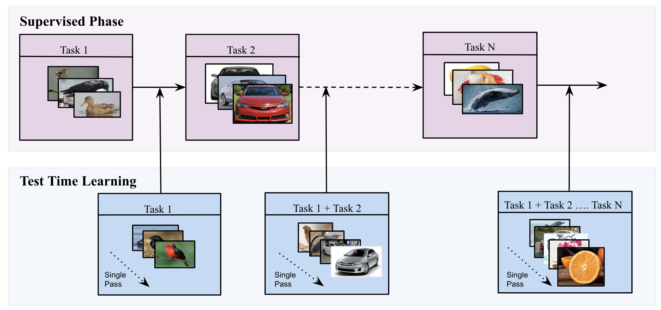
After training is complete on each the model is put into production until becomes available for supervised training. Between supervised phases an unsupervised dataset, , is observed corresponding to test-time data encountered in production. Note that this unsupervised data can be drawn from a different distribution than the supervised data, including the distributions of old supervised datasets/tasks. Our goal is to leverage this data to control forgetting of the model by allowing online unsupervised adaptation. Figure 1 depicts our setting. Note that we evaluate our models on test datasets that are distinct in terms of instances from those used during the self-supervised online adaptation phase to adequately measure models generalization.
We further note that although supervised phases may permit multiple passes through the data until convergence, it would be impractical to collect unsupervised data in production and then perform adaptation on it, we thus restrict the unsupervised phase to be in the online setting [48, 19, 6]. This is especially important in cases were data privacy is important e.g., assistant robot in a private smart home environment.
3.2 DoSAPP: Double Smoothing via Affine Projected Parameters
We propose a simple yet effective method for continual test-time learning, Double Smoothing via Affine Projected Parameters aka DoSAPP. Our approach combines two key components: 1) sparse and local updates: to reduce forgetting, maintain generalization, and ensure efficient updates, and 2) teacher-student framework to promote stability in online updates and minimizes forgetting. In the continual test time learning we can identify two distinct phases of learning as outlined in the following.
Phase 1: Continual Learning Supervised Training with Sparse Selected Parameters
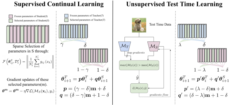
Our primary objective is to swiftly accumulate new knowledge without catastrophically forgetting the generic knowledge both at training and test-time. To achieve this, we opt for updating only a small subset of selected parameters. It has been suggested by Zhang et al. [64] that for a generic prertrained model like CLIP and a given task, relevant parameters can be identified before training, and updating only those parameters would result in a reduced forgetting of previous knowledge. Further Geva et al. [14]suggested that MLP blocks in a transformer model emulate key-value neural memories, where the first layer of MLP acts as memory keys operating as pattern detectors. This suggests that for updating knowledge of previously known ”patterns”, it might be sufficient to update only first MLP layer parameters. Thus we limit candidate parameters to the first MLP layer parameters of each transformer block in the CLIP model [64]. From these candidate parameters of the first MLP layer of each transformer, we select top-K(K=) parameters. This results in efficient training without loss of previously acquired knowledge as all other layers remain frozen.
Following [64] we use the gradient magnitude of the loss w.r.t. the incoming data as a score of how relevant a parameter is, the larger the gradient magnitude the larger the expected decrease in loss after small changes to that parameter. We refer to the model being optimized as . Upon recieving supervised data, we first estimate the most relevant parameters, such that ().
| (2) |
where is the gradient of the loss function() regarding the parameter evaluated at the data point and its label . The loss function is the same CLIP loss, and the entire data is iterated once to compute the gradient score as given in Eq 2. Specifying the sparsity threshold(), top-K(K=) most relevant parameters are selected. We set as shown in [64]. This results in a binary mask m where only selected parameters are updated and others are masked out and kept frozen.
Teacher Student Framework
To insure stability later during online updates and reduce forgetting, we utilise a Student-Teacher framework [50, 23, 4] where the student model is denoted by and the teacher model is denoted by .
During both train and test time, teacher model parameters move with exponentially moving average (EMA) of student model parameters . Normally in a teacher student framework, all teacher model parameters move similarly towards the student parameters with a single smoothing parameter (momentum). However, in tables 1 and 4 we show that a single smoothing parameter is insufficient and yields poor performance. Indeed, in our case most of student model parameters remain frozen and only a small portion is updated, we propose that teacher model’s parameters corresponding to the student frozen parameters should move at a different pace than those selected for updates. Therefore we use dual smoothing parameters (referred as momentum parameters) based on affine transformation of the binary mask m to adapt the teacher parameters .
Weighted exponential smoothing with dual momentum
After each gradient update step() for , parameters of are updated by EMA of the student model parameters. Typically, EMA is governed by
| (3) |
where is the smoothing parameter. Further it has been shown in ([50, 35, 23]) that setting to a high value(eg 0.9999), maintains a stable teacher model that can be considered as a strong reference for past tasks . But updating the teacher model with single smoothing parameter in case where parameters are masked creates a dissonance and increases forgetting because all the parameters are updated with equal importance, disregarding those parameters which are selected by the gradient scoring function(where ). To account for masking, we modify Eq 3 as
| (4) |
where and denote the smoothing parameters for the teacher and student model respectively, and can be computed as
| (5) | |||
where . This means that the selected parameters of the teacher model ([]), move little bit faster towards the student model as compared to the frozen parameters(where []). As such, parameters where [] will move at a slow rate of and unmasked parameters would be updated with . When , the weighted scheme becomes EMA with single smoothing parameter. A detailed proof is given in appendix A.1.
Phase 2: Unsupervised Test Time Learning(TTL)
After supervised training is completed, both and are deployed for Test Time Learning(TTL). We consider teacher() and student() models as two experts on different data distributions, the on the most recent and the on previous sessions distributions.
We take inspiration from Out Of Distribution (ODD) literature [17], where a sample has to be identified as In Distribution (ID) for a given predictor with a score function predicting high values for ID samples as opposed to OOD samples. Recently it has been shown that using the un-normalized maximum logit output of a given predictor as an ID score is significantly more robust than softmax probability [18]. Indeed the softmax probability is shown to provide high probability predictions even for unknown samples [62], which we want to avoid in our case. Note that for CLIP the logit corresponds to the cosine similarity of image batch with given text features.
Following [18], we use maximum logit value of each expert as an ID score, and select for each test sample the expert with the highest ID score indicating that the sample is likely to be better represented by said expert. We then accept the pseudo label of the selected expert. Formally the pseudo label can be calculated as follows:
| (6) |
where is the accepted pseudo label and and are the maximum logit score for teacher and student model respectively,
| Momentum(, ) | Aircraft | ||
| Acc. () | F.() | FTA. () | |
| 0.9999, 0.9999 | 23.99 | 18.36 | 12.15 |
| 0.5, 0.9 | 38.41 | 3.27 | 37.64 |
| 0.7, 0.9 | 37.22 | 3.05 | 37.72 |
| 0.8, 0.9* | 39.40 | 2.61 | 38.13 |
| 0.8, 0.6 | 37.06 | 5.12 | 29.63 |
| 0.8, 0.5 | 32.95 | 3.40 | 26.33 |
and similarly and are the pseudo labels by teacher and student models respectively. During test-time training the student model is updated by minimising CLIP contrastive loss given pseudo label . In realistic settings, often multiple iterations on test data is not always possible, for eg, a streaming data pipeline. We too mimic this setting, where the entire data is processed only once during TTL phase.
Similar to the above mentioned supervised phase, we also here apply sparse local updates to . However, estimation of masks based on the online data might be noisy, and largely reduce the efficiency as gradients of all parameters must be estimated for each mini batch of test samples. To overcome this, and following the assumption that test data are drawn from the distributions of all previous tasks, we leverage the masks estimated for previous tasks. We accumulate a union of the binary masks () over all the previously seen tasks such that . To maintain the same sparsity level () of performed updates, we further select the same top-K (K=) most relevant parameters, from these new masked parameters based on their previously computed gradient scores.
Finally is updated using the same dual momentum scheme, but with different smoothing vectors as:
| (7) |
where and . In TTL phase, the momentum parameter is kept such that . This means that moves more slowly in direction of during TTL phase as compared to the supervised phase. As we encounter frequent, and possibly noisy, online updates, stability is better insured by a slower pace of movements towards student parameters. We show the sensitivity of our method on choice of momentum values in table 1. A high has been chosen to keep the Teacher model stable as shown in [50, 35, 23]. It can be clearly seen that when (single momentum EMA), the performance significantly drops. DoSAPP is less sensitive to on chocie of , but it highly depends on . We can also see that as , the performance again drops. The algorithm can be fully understood as given in 1
4 Experiments
4.1 Setup
Architecture: We apply DoSAPP to vision-language classification tasks, given their relatively robust knowledge measurement in such tasks. CLIP-ViT/B-16 [40], is used as backbone. We report the accuracies recorded by the Teacher model. We refer to [64] for hyperparameters selection other than dual momentums, which are given in Appendix A.2.
Datasets: We consider five different vision datasets, three fine-grained(Aircraft[30], CUB[53], Stanford Cars[24], Oxford Pets[36], one coarse dataset(CIFAR100 [25]) and one out-of-distribution dataset(GSTRB[47]). These datasets are chosen primarily based on their initially low zero-shot performance with CLIP pre-trained models. To form the continual learning sequences, we split each dataset into 10 subsets with disjoint classes composing 10 tasks. For all the datasets, the training data is used in supervised learning phase. The test data is divided into 2 splits, namely where is utilised for test-time unsupervised learning and is used for evaluation.
Evaluation Metrics: After each supervised session and the following test-time adaptation session, we evaluate the model test performance on holdout datasets from all tasks. In order to do this, we construct the matrix , where is the test classification accuracy of the model on task after observing the last sample from task . Thus, we compute Average Accuracy(Acc. = ) and Average Forgetting(F. = ) [29]. Taken together, these two metrics allow us to assess how well a continual learner solves a classification problem while overcoming forgetting. All experiments have been done on NVIDIA A100 GPU and each one takes approximately 1 hour for completion.
| Method | Aircraft | Cars | CIFAR100 | CUB | GTSRB | |||||
|---|---|---|---|---|---|---|---|---|---|---|
| Acc. () | F.() | Acc. () | F.() | Acc. () | F.() | Acc. () | F.() | Acc. () | F.() | |
| CLIP-Zeroshot [40] | 24.45 | - | 64.63 | - | 68.25 | - | 55.13 | - | 43.38 | - |
| Finetune [15] | 18.63 | 39.93 | 51.64 | 25.65 | 46.26 | 37.78 | 45.74 | 26.62 | 21.76 | 55.48 |
| SL | 10.81 | 50.81 | 23.49 | 30.42 | 38.03 | 42.67 | 28.60 | 33.82 | 5.14 | 62.31 |
| MAS [1] | 33.69 | 27.50 | 69.43 | 9.18 | 63.88 | 21.16 | 61.72 | 12.05 | 42.04 | 25.38 |
| L2P[61] | 32.20 | 21.73 | 67.04 | 11.22 | 67.71 | 18.81 | 64.04 | 6.82 | 75.45 | 2.68 |
| DualPrompt [60] | 26.61 | 17.20 | 63.30 | 18.67 | 61.72 | 19.87 | 64.38 | 12.94 | 69.65 | 8.43 |
| SLCA [63] | 29.40 | 11.45 | 62.65 | 4.42 | 70.03 | 0.19 | 53.87 | 7.75 | 46.01 | 0.83 |
| ZSCL [65] | 30.96 | 15.65 | 67.79 | 8.27 | 80.50 | 1.05 | 61.09 | 7.69 | 62.92 | 13.54 |
| SparseCL [59] | 31.95 | 19.77 | 71.57 | 5.38 | 69.35 | 15.23 | 62.50 | 9.66 | 48.99 | 24.91 |
| SPU [64] | 30.94 | 28.36 | 69.41 | 16.91 | 58.80 | 26.37 | 62.31 | 7.2 | 43.06 | 19.16 |
| DoSAPP | 39.14 | 12.55 | 74.87 | -0.74 | 79.16 | 7.73 | 68.17 | 2.15 | 72.33 | 1.02 |
| ER methods | ||||||||||
| ER[13] | 41.42 | 31.38 | 69.08 | 16.42 | 82.86 | 3.41 | 64.07 | 17.72 | 96.28 | -7.48 |
| ER + LWF[28] | 36.08 | 18.12 | 72.56 | 4.04 | 74.32 | 8.16 | 65.11 | 5.90 | 53.56 | 11.86 |
| ER + PRD [2] | 37.11 | 17.35 | 74.08 | 3.75 | 79.66 | 3.10 | 65.92 | 6.55 | 63.00 | 12.44 |
| SPU + ER=1000 | 44.43 | 14.42 | 77.51 | 3.26 | 83.99 | -0.39 | 71.51 | 4.84 | 94.25 | -7.87 |
| DoSAPP + ER=200 | 47.32 | 8.10 | 79.17 | 3.92 | 88.41 | -1.96 | 74.39 | 2.77 | 83.67 | 1.92 |
4.2 Results
We compare variety of baselines with our proposed method in table. 2. Along with the methods mentioned in table. 2, we also compare our method with self labeling(SL) where the groundtruth pseudo label comes from the trained model itself(without any student-teacher framework). When comparing methods without ER, DoSAPP achieves state of the art results in all the five datasets used in the experiments. This highlights the fact that test time data can be utilised for improving transferability as well as preserving previously learned knowledge. Even when comparing methods with ER, DoSAPP(without ER) gives a comparable performance in almost all the datasets. We note that SPU+ER employs a very high buffer of 1000, which attributes to such a high performance in some datasets like Cifar100 and GTSRB. Although our method is robust enough to be used without ER and our primary motivation is to circumvent the usage of buffer, but we still present results with a small buffer(DoSAPP+ER, ER=200), for a comparison to the baselines using ER. DoSAPP + ER outperforms all other baselines except on GTSRB by significant margin.
4.3 Class Incremental Long Sequence scenario with domain shift
We also consider the case where we have a long sequence of tasks each to be trained in a class incremental fashion. For these experiments, we combined the 10 tasks of Aircraft data[30] and 10 tasks of Cars data[24]. This firstly creates a long sequence of tasks in a class incremental scenario, and secondly causes a domain shift after 10 tasks of aircraft. From table 3, it can be clearly seen that our proposed method DoSAPP outperforms SPU without ER and Finetune(without any TTL phase). Further it can be inferred that in other baselines, there is a recency bias towards the current task, whereas in DoSAPP, with a marginal decrease of on current task accuracy(CTA), there is an overall increase in the average accuracy and the first task accuracy. This shows that our approach retains the knowledge on first task as well adapts well on the current task, with strong generalisation performance.
| Method(CLIP) | Avg Acc | FTA | CTA |
|---|---|---|---|
| Finetune(no TTL) | 35.24 0.87 | 5.90 1.20 | 75.44 0.52 |
| SPU | 39.62 1.62 | 24.31 0.30 | 74.94 2.43 |
| DoSAPP | 45.01 0.31 | 30.63 0. 76 | 71.13 1.17 |
5 Ablation Study
In this section we quantitatively analyse the effect of different components of our proposed method DoSAPP. We evaluate the effects of each component in an incremental fashion as seen in table. 4. Starting with only a student and teacher model setup only, we subject it to TTL data and this forms our baseline. Next we compare with localised sparse updates for the first MLP layer of each of the transformer blocks. This gives an increase in performance in 4 out of 5 datasets. It is to be noted that the momentum used to update the teacher model is according to Eq. 3. We then take the union of supervised task masks to use them at TTL phase, but this deteriorates performance since the masked parameters and unmasked parameters are updated with a single momentum. Finally we add our dual momentum approach which gives best performance. We also subject our approach to a more challenging scenario where the tasks in TTL phases are class-imbalanced. Here we sample each task from a symmetric Dirichlet distribution whose concentration parameter is the length of each task. This causes a high imbalance of classes within each task, and sometimes, even absence of certain classes. This imbalanced case is of particular importance since in real settings, test suites are often skewed.This is done by randomly sampling classes from a Dirichlet’s distribution. Although the performance is inferior to the balanced case, it should not be interpreted as a drawback. This is because, the model should adapt more to the classes that are seen often in TTL phases and loss of performance on rarely seen classes is but natural.
| Components of DoSAPP | Aircraft | Cars | CIFAR100 | CUB | GTSRB | |||||
|---|---|---|---|---|---|---|---|---|---|---|
| Acc. () | F.() | Acc. () | F.() | Acc. () | F.() | Acc. () | F.() | Acc. () | F.() | |
| Only Teacher-Student | 30.12 | 3.50 | 67.72 | 3.66 | 77.82 | 5.17 | 62.67 | 4.11 | 53.57 | 5.38 |
| + sparse params | 34.16 | 8.61 | 69.42 | 3.41 | 71.93 | 8.24 | 66.32 | 3.98 | 55.32 | 5.81 |
| + union of mask | 32.99 | 10.36 | 67.48 | 6.91 | 76.77 | 10.11 | 65.70 | 26.62 | 56.82 | 3.21 |
| +dual momentum* | 39.14 | 2.55 | 74.87 | -0.74 | 79.16 | 7.73 | 68.17 | 2.15 | 72.33 | 1.02 |
| + imbalanced TTL | 35.99 | 5.22 | 72.68 | 6.38 | 75.70 | 9.81 | 64.84 | 3.73 | 68.17 | 5.63 |
6 Limitation
DoSAPP is a robust algorithm which can be potentially applied to any CL technique for unsupervised adaptation of Test Time Data. However, since it utilises the test data, its primary bottleneck becomes the quality of test data especially if its highyly skewed. Another limitation is the increase in the computational budget due to two deployed models: Student-Teacher framework. We address this by leveraging efficient sparse parameter selection method.
7 Discussion and Conclusion
In this work, we discuss how to leverage test-time data to improve models’ representation of previous tasks, mimicking human learning and striving for real intelligent agents. In summary, to the best of our knowledge we are the first to explore test-time learning to control forgetting. We show that test-time data can provide a great source of information when leveraged correctly. Our method, DoSAPP, was able to significantly improve over the zero-shot performance of CLIP when continually learning a dataset without any replay and with no specific CL method applied at the supervised training session. DoSAPP is stable due to sparse parameter updates and the weighted EMA teacher-student framework. Further during TTL, the max-logit in distribution scores makes it more robust to class imbalance than other strategies.
8 Acknowledgements
E.B. and V.S. acknowledge funding from NSERC Discovery Grant RGPIN- 2021-04104. This research was enabled in part by compute resources provided by Digital Research Alliance of Canada (the Alliance) and Calcul Québec.
References
- Aljundi et al. [2018] R. Aljundi, F. Babiloni, M. Elhoseiny, M. Rohrbach, and T. Tuytelaars. Memory aware synapses: Learning what (not) to forget. In European Conference on Computer Vision (ECCV), 2018.
- Asadi et al. [2023] N. Asadi, M. Davari, S. Mudur, R. Aljundi, and E. Belilovsky. Prototype-sample relation distillation: towards replay-free continual learning. In International Conference on Machine Learning, pages 1093–1106. PMLR, 2023.
- Bommasani et al. [2021] R. Bommasani, D. A. Hudson, E. Adeli, R. Altman, S. Arora, S. von Arx, M. S. Bernstein, J. Bohg, A. Bosselut, E. Brunskill, et al. On the opportunities and risks of foundation models. arXiv preprint arXiv:2108.07258, 2021.
- Boschini et al. [2022] M. Boschini, L. Bonicelli, A. Porrello, G. Bellitto, M. Pennisi, S. Palazzo, C. Spampinato, and S. Calderara. Transfer without forgetting. In European Conference on Computer Vision, pages 692–709. Springer, 2022.
- Brown et al. [2020] T. B. Brown, B. Mann, N. Ryder, M. Subbiah, J. Kaplan, P. Dhariwal, A. Neelakantan, P. Shyam, G. Sastry, A. Askell, S. Agarwal, A. Herbert-Voss, G. Krueger, T. Henighan, R. Child, A. Ramesh, D. M. Ziegler, J. Wu, C. Winter, C. Hesse, M. Chen, E. Sigler, M. Litwin, S. Gray, B. Chess, J. Clark, C. Berner, S. McCandlish, A. Radford, I. Sutskever, and D. Amodei. Language models are few-shot learners. In Proceedings of the 34th International Conference on Neural Information Processing Systems, NIPS’20, 2020.
- Cai et al. [2021] Z. Cai, O. Sener, and V. Koltun. Online continual learning with natural distribution shifts: An empirical study with visual data. In Proceedings of the IEEE/CVF international conference on computer vision, pages 8281–8290, 2021.
- Caron et al. [2021] M. Caron, H. Touvron, I. Misra, H. J’egou, J. Mairal, P. Bojanowski, and A. Joulin. Emerging properties in self-supervised vision transformers. 2021 ieee. In CVF International Conference on Computer Vision (ICCV), volume 3, 2021.
- Chen et al. [2022] D. Chen, D. Wang, T. Darrell, and S. Ebrahimi. Contrastive test-time adaptation. In Proceedings of the IEEE/CVF Conference on Computer Vision and Pattern Recognition, pages 295–305, 2022.
- Chen et al. [2023] J. Chen, D. Zhu, X. Shen, X. Li, Z. Liu, P. Zhang, R. Krishnamoorthi, V. Chandra, Y. Xiong, and M. Elhoseiny. Minigpt-v2: large language model as a unified interface for vision-language multi-task learning. arXiv preprint arXiv:2310.09478, 2023.
- De Lange et al. [2021] M. De Lange, R. Aljundi, M. Masana, S. Parisot, X. Jia, A. Leonardis, G. Slabaugh, and T. Tuytelaars. A continual learning survey: Defying forgetting in classification tasks. IEEE transactions on pattern analysis and machine intelligence, 44(7):3366–3385, 2021.
- Ding et al. [2022] Y. Ding, L. Liu, C. Tian, J. Yang, and H. Ding. Don’t stop learning: Towards continual learning for the clip model. arXiv preprint arXiv:2207.09248, 2022.
- Ermis et al. [2022] B. Ermis, G. Zappella, M. Wistuba, A. Rawal, and C. Archambeau. Memory efficient continual learning with transformers. Advances in Neural Information Processing Systems, 35:10629–10642, 2022.
- French [1999] R. French. Catastrophic forgetting in connectionist networks. Trends in cognitive sciences, 3:128–135, 1999.
- Geva et al. [2020] M. Geva, R. Schuster, J. Berant, and O. Levy. Transformer feed-forward layers are key-value memories. arXiv preprint arXiv:2012.14913, 2020.
- Goyal et al. [2023] S. Goyal, A. Kumar, S. Garg, Z. Kolter, and A. Raghunathan. Finetune like you pretrain: Improved finetuning of zero-shot vision models. In Proceedings of the IEEE/CVF Conference on Computer Vision and Pattern Recognition, pages 19338–19347, 2023.
- Han et al. [2021] X. Han, Z. Zhang, N. Ding, Y. Gu, X. Liu, Y. Huo, J. Qiu, Y. Yao, A. Zhang, L. Zhang, et al. Pre-trained models: Past, present and future. AI Open, 2:225–250, 2021.
- Hendrycks and Gimpel [2016] D. Hendrycks and K. Gimpel. A baseline for detecting misclassified and out-of-distribution examples in neural networks. arXiv preprint arXiv:1610.02136, 2016.
- Hendrycks et al. [2019] D. Hendrycks, S. Basart, M. Mazeika, A. Zou, J. Kwon, M. Mostajabi, J. Steinhardt, and D. Song. Scaling out-of-distribution detection for real-world settings. arXiv preprint arXiv:1911.11132, 2019.
- Jang et al. [2022] M. Jang, S.-Y. Chung, and H. W. Chung. Test-time adaptation via self-training with nearest neighbor information. arXiv preprint arXiv:2207.10792, 2022.
- Janson et al. [2022] P. Janson, W. Zhang, R. Aljundi, and M. Elhoseiny. A simple baseline that questions the use of pretrained-models in continual learning. arXiv preprint arXiv:2210.04428, 2022.
- Kirkpatrick et al. [2017a] J. Kirkpatrick, R. Pascanu, N. Rabinowitz, J. Veness, G. Desjardins, A. A. Rusu, K. Milan, J. Quan, T. Ramalho, A. Grabska-Barwinska, et al. Overcoming catastrophic forgetting in neural networks. Proceedings of the national academy of sciences, 114(13):3521–3526, 2017a.
- Kirkpatrick et al. [2017b] J. Kirkpatrick, R. Pascanu, N. Rabinowitz, J. Veness, G. Desjardins, A. A. Rusu, K. Milan, J. Quan, T. Ramalho, A. Grabska-Barwinska, et al. Overcoming catastrophic forgetting in neural networks. Proceedings of the national academy of sciences, 114(13):3521–3526, 2017b.
- Koh et al. [2022] H. Koh, M. Seo, J. Bang, H. Song, D. Hong, S. Park, J.-W. Ha, and J. Choi. Online boundary-free continual learning by scheduled data prior. In The Eleventh International Conference on Learning Representations, 2022.
- Krause et al. [2013] J. Krause, M. Stark, J. Deng, and L. Fei-Fei. 3d object representations for fine-grained categorization. In Proceedings of the IEEE international conference on computer vision workshops, pages 554–561, 2013.
- Krizhevsky [2012] A. Krizhevsky. Learning multiple layers of features from tiny images. University of Toronto, 05 2012.
- Li et al. [2022] J. Li, D. Li, C. Xiong, and S. Hoi. Blip: Bootstrapping language-image pre-training for unified vision-language understanding and generation. In International Conference on Machine Learning, pages 12888–12900. PMLR, 2022.
- Li and Hoiem [2017a] Z. Li and D. Hoiem. Learning without forgetting. IEEE transactions on pattern analysis and machine intelligence, 40(12):2935–2947, 2017a.
- Li and Hoiem [2017b] Z. Li and D. Hoiem. Learning without forgetting. IEEE transactions on pattern analysis and machine intelligence, 40(12):2935–2947, 2017b.
- Lopez-Paz and Ranzato [2017] D. Lopez-Paz and M. Ranzato. Gradient episodic memory for continual learning. Advances in neural information processing systems, 30, 2017.
- Maji et al. [2013] S. Maji, J. Kannala, E. Rahtu, M. Blaschko, and A. Vedaldi. Fine-grained visual classification of aircraft. Technical report, 2013.
- Maltoni and Lomonaco [2019] D. Maltoni and V. Lomonaco. Continuous learning in single-incremental-task scenarios. Neural Networks, 116:56–73, 2019.
- McCloskey and Cohen [1989] M. McCloskey and N. J. Cohen. Catastrophic interference in connectionist networks: The sequential learning problem. In Psychology of learning and motivation, volume 24, pages 109–165. Elsevier, 1989.
- Nado et al. [2020] Z. Nado, S. Padhy, D. Sculley, A. D’Amour, B. Lakshminarayanan, and J. Snoek. Evaluating prediction-time batch normalization for robustness under covariate shift. arXiv preprint arXiv:2006.10963, 2020.
- Niu et al. [2023] S. Niu, J. Wu, Y. Zhang, Z. Wen, Y. Chen, P. Zhao, and M. Tan. Towards stable test-time adaptation in dynamic wild world. arXiv preprint arXiv:2302.12400, 2023.
- Oquab et al. [2023] M. Oquab, T. Darcet, T. Moutakanni, H. Vo, M. Szafraniec, V. Khalidov, P. Fernandez, D. Haziza, F. Massa, A. El-Nouby, et al. Dinov2: Learning robust visual features without supervision. arXiv preprint arXiv:2304.07193, 2023.
- Parkhi et al. [2012] O. M. Parkhi, A. Vedaldi, A. Zisserman, and C. Jawahar. Cats and dogs. In 2012 IEEE conference on computer vision and pattern recognition, pages 3498–3505. IEEE, 2012.
- Pei et al. [2023] R. Pei, J. Liu, W. Li, B. Shao, S. Xu, P. Dai, J. Lu, and Y. Yan. Clipping: Distilling clip-based models with a student base for video-language retrieval. In Proceedings of the IEEE/CVF Conference on Computer Vision and Pattern Recognition, pages 18983–18992, 2023.
- Pelosin [2022] F. Pelosin. Simpler is better: off-the-shelf continual learning through pretrained backbones. arXiv preprint arXiv:2205.01586, 2022.
- Prabhu et al. [2023] A. Prabhu, H. A. Al Kader Hammoud, P. K. Dokania, P. H. Torr, S.-N. Lim, B. Ghanem, and A. Bibi. Computationally budgeted continual learning: What does matter? In Proceedings of the IEEE/CVF Conference on Computer Vision and Pattern Recognition, pages 3698–3707, 2023.
- Radford et al. [2021a] A. Radford, J. W. Kim, C. Hallacy, A. Ramesh, G. Goh, S. Agarwal, G. Sastry, A. Askell, P. Mishkin, J. Clark, et al. Learning transferable visual models from natural language supervision. In International conference on machine learning, pages 8748–8763. PMLR, 2021a.
- Radford et al. [2021b] A. Radford, J. W. Kim, C. Hallacy, A. Ramesh, G. Goh, S. Agarwal, G. Sastry, A. Askell, P. Mishkin, J. Clark, et al. Learning transferable visual models from natural language supervision. In International conference on machine learning, pages 8748–8763. PMLR, 2021b.
- Rasheed et al. [2023] H. Rasheed, M. U. Khattak, M. Maaz, S. Khan, and F. S. Khan. Fine-tuned clip models are efficient video learners. In Proceedings of the IEEE/CVF Conference on Computer Vision and Pattern Recognition, pages 6545–6554, 2023.
- Ridnik et al. [2021] T. Ridnik, E. Ben-Baruch, A. Noy, and L. Zelnik-Manor. Imagenet-21k pretraining for the masses. arXiv preprint arXiv:2104.10972, 2021.
- Schwarz et al. [2018] J. Schwarz, W. Czarnecki, J. Luketina, A. Grabska-Barwinska, Y. W. Teh, R. Pascanu, and R. Hadsell. Progress & compress: A scalable framework for continual learning. In International Conference on Machine Learning, pages 4528–4537. PMLR, 2018.
- Shin et al. [2017] H. Shin, J. K. Lee, J. Kim, and J. Kim. Continual learning with deep generative replay. Advances in neural information processing systems, 30, 2017.
- Smith et al. [2023] J. S. Smith, L. Karlinsky, V. Gutta, P. Cascante-Bonilla, D. Kim, A. Arbelle, R. Panda, R. Feris, and Z. Kira. Coda-prompt: Continual decomposed attention-based prompting for rehearsal-free continual learning. In Proceedings of the IEEE/CVF Conference on Computer Vision and Pattern Recognition, pages 11909–11919, 2023.
- Stallkamp et al. [2012] J. Stallkamp, M. Schlipsing, J. Salmen, and C. Igel. Man vs. computer: Benchmarking machine learning algorithms for traffic sign recognition. Neural networks, 32:323–332, 2012.
- Sun et al. [2020a] Y. Sun, X. Wang, Z. Liu, J. Miller, A. Efros, and M. Hardt. Test-time training with self-supervision for generalization under distribution shifts. In International conference on machine learning, pages 9229–9248. PMLR, 2020a.
- Sun et al. [2020b] Y. Sun, X. Wang, Z. Liu, J. Miller, A. Efros, and M. Hardt. Test-time training with self-supervision for generalization under distribution shifts. In International conference on machine learning, pages 9229–9248. PMLR, 2020b.
- Tarvainen and Valpola [2017] A. Tarvainen and H. Valpola. Mean teachers are better role models: Weight-averaged consistency targets improve semi-supervised deep learning results. Advances in neural information processing systems, 30, 2017.
- Verwimp et al. [2023] E. Verwimp, S. Ben-David, M. Bethge, A. Cossu, A. Gepperth, T. L. Hayes, E. Hüllermeier, C. Kanan, D. Kudithipudi, C. H. Lampert, et al. Continual learning: Applications and the road forward. arXiv preprint arXiv:2311.11908, 2023.
- Vianna et al. [2024] P. Vianna, M. Chaudhary, P. Mehrbod, A. Tang, G. Cloutier, G. Wolf, M. Eickenberg, and E. Belilovsky. Channel-selective normalization for label-shift robust test-time adaptation. arXiv preprint arXiv:2402.04958, 2024.
- Wah et al. [2011] C. Wah, S. Branson, P. Welinder, P. Perona, and S. Belongie. The caltech-ucsd birds-200-2011 dataset. Technical report, California Institute of Technology, 2011.
- Wang et al. [2020] D. Wang, E. Shelhamer, S. Liu, B. Olshausen, and T. Darrell. Tent: Fully test-time adaptation by entropy minimization. arXiv preprint arXiv:2006.10726, 2020.
- Wang et al. [2024] L. Wang, X. Zhang, H. Su, and J. Zhu. A comprehensive survey of continual learning: Theory, method and application. IEEE Transactions on Pattern Analysis and Machine Intelligence, 2024.
- Wang et al. [2022a] Q. Wang, O. Fink, L. Van Gool, and D. Dai. Continual test-time domain adaptation. In Proceedings of the IEEE/CVF Conference on Computer Vision and Pattern Recognition, pages 7201–7211, 2022a.
- Wang et al. [2022b] Q. Wang, O. Fink, L. Van Gool, and D. Dai. Continual test-time domain adaptation. In Proceedings of the IEEE/CVF Conference on Computer Vision and Pattern Recognition, pages 7201–7211, 2022b.
- Wang et al. [2022c] Y. Wang, Z. Huang, and X. Hong. S-prompts learning with pre-trained transformers: An occam’s razor for domain incremental learning. Advances in Neural Information Processing Systems, 35:5682–5695, 2022c.
- Wang et al. [2022d] Z. Wang, Z. Zhan, Y. Gong, G. Yuan, W. Niu, T. Jian, B. Ren, S. Ioannidis, Y. Wang, and J. Dy. Sparcl: Sparse continual learning on the edge. Advances in Neural Information Processing Systems, 35:20366–20380, 2022d.
- Wang et al. [2022e] Z. Wang, Z. Zhang, S. Ebrahimi, R. Sun, H. Zhang, C.-Y. Lee, X. Ren, G. Su, V. Perot, J. Dy, et al. Dualprompt: Complementary prompting for rehearsal-free continual learning. In European Conference on Computer Vision, pages 631–648. Springer, 2022e.
- Wang et al. [2022f] Z. Wang, Z. Zhang, C.-Y. Lee, H. Zhang, R. Sun, X. Ren, G. Su, V. Perot, J. Dy, and T. Pfister. Learning to prompt for continual learning. In Proceedings of the IEEE/CVF Conference on Computer Vision and Pattern Recognition, pages 139–149, 2022f.
- Yang et al. [2021] J. Yang, K. Zhou, Y. Li, and Z. Liu. Generalized out-of-distribution detection: A survey. arXiv preprint arXiv:2110.11334, 2021.
- Zhang et al. [2023a] G. Zhang, L. Wang, G. Kang, L. Chen, and Y. Wei. Slca: Slow learner with classifier alignment for continual learning on a pre-trained model. arXiv preprint arXiv:2303.05118, 2023a.
- Zhang et al. [2023b] W. Zhang, P. Janson, R. Aljundi, and M. Elhoseiny. Overcoming generic knowledge loss with selective parameter update. arXiv preprint arXiv:2308.12462, 2023b.
- Zheng et al. [2023] Z. Zheng, M. Ma, K. Wang, Z. Qin, X. Yue, and Y. You. Preventing zero-shot transfer degradation in continual learning of vision-language models. In Proceedings of the IEEE/CVF International Conference on Computer Vision, pages 19125–19136, 2023.
- Zhou et al. [2022] D.-W. Zhou, Q.-W. Wang, H.-J. Ye, and D.-C. Zhan. A model or 603 exemplars: Towards memory-efficient class-incremental learning. arXiv preprint arXiv:2205.13218, 2022.
- Zhou et al. [2023] D.-W. Zhou, H.-J. Ye, D.-C. Zhan, and Z. Liu. Revisiting class-incremental learning with pre-trained models: Generalizability and adaptivity are all you need. arXiv preprint arXiv:2303.07338, 2023.
Appendix A Appendix / supplemental material
A.1 Derivation for dual momentum
In section 3, the teacher model parameters undergo exponential moving average as
| (8) |
where and denote the smoothing parameters for the teacher and student model respectively, and can be computed as
| (9) | |||
where and for are the coefficients for affine transformation of the boolean mask vector m.
To account for masked parameters, two momentum values are introduced for teacher and student models respectively, such that for the teacher model, affine coefficients are computed by solving the equations:
| (10) |
and are computed by solving the equations
| (11) |
This gives
| (12) | |||
This gives
| (13) | |||
A.2 Hyperparameters
tablele 5 shows different hyperparameters that have been used for all the experiments using CLIP backbones. The hyperparameters were selected based on the performance of the first task of Stanford Cars dataset. All the results have been gathered over experiments averaged over 5 random seeds.
| Hparams | CLIP model |
|---|---|
| Batch Size | 64 |
| Optimizer | AdamW |
| Learning Rate | |
| CL Epochs | 10 |
| Buffer | 0 |
| TTL batch size | 64 |
| Momentum-EMA() | 0.9999, 0.8, 0.9 |
| sparsity() | 0.1 |