Improving GFlowNets with Monte Carlo Tree Search
Abstract
Generative Flow Networks (GFlowNets) treat sampling from distributions over compositional discrete spaces as a sequential decision-making problem, training a stochastic policy to construct objects step by step. Recent studies have revealed strong connections between GFlowNets and entropy-regularized reinforcement learning. Building on these insights, we propose to enhance planning capabilities of GFlowNets by applying Monte Carlo Tree Search (MCTS). Specifically, we show how the MENTS algorithm (Xiao et al., 2019) can be adapted for GFlowNets and used during both training and inference. Our experiments demonstrate that this approach improves the sample efficiency of GFlowNet training and the generation fidelity of pre-trained GFlowNet models.
1 Introduction
Generative Flow Networks (GFlowNets, Bengio et al., 2021) are models designed to sample compositional discrete objects, such as graphs, from distributions defined by unnormalized probability mass functions. They achieve this by training a stochastic policy to generate objects through a sequence of constructive actions to match the desired distribution. GFlowNets have been successfully applied in various areas, including biological sequence design (Jain et al., 2022), large language model (LLM) fine-tuning (Hu et al., 2023), combinatorial optimization (Zhang et al., 2023), neural architecture search (Chen & Mauch, 2023), and causal discovery (Atanackovic et al., 2024).
GFlowNets incorporate many concepts and techniques from reinforcement learning (RL). Recent works (Tiapkin et al., 2024; Mohammadpour et al., 2024; Deleu et al., 2024) have shown that the GFlowNet learning problem can be reformulated as an RL problem with entropy regularization (Neu et al., 2017; Geist et al., 2019). These findings opened a direct way to apply many existing RL algorithms (Schulman et al., 2017; Haarnoja et al., 2017, 2018) to GFlowNets, and our work follows this path.
Monte Carlo Tree Search (MCTS) is a well-known method for solving planning problems (Coulom, 2006; Kocsis & Szepesvári, 2006). Prominent examples of RL algorithms utilizing MCTS include AlphaGo (Silver et al., 2016) and AlphaZero (Silver et al., 2018), which combine MCTS with deep neural networks to achieve superhuman performance in games like Go, chess, and Shogi. MCTS algorithms typically require knowledge of the environment’s underlying dynamics or can be paired with a neural network-based simulator, as seen in MuZero-type approaches (Schrittwieser et al., 2020), resulting in a complicated algorithm. Fortunately, GFlowNets fall into the first category because the directed acyclic graph (DAG) environments they operate in are integral to the algorithm’s design and, moreover, deterministic. Thus, the ability to simulate any trajectory in a deterministic DAG environment makes the idea of enhancing the planning abilities of GFlowNets with MCTS very natural.
We focus on the Maximum Entropy for Tree Search (MENTS, Xiao et al., 2019) algorithm, an MCTS algorithm that estimates entropy-regularized Q-values. This entropy-regularized nature of this algorithm allows it to be directly applied to the framework of GFlowNets. We outline our contributions as follows: i) We show how MENTS coupled with SoftDQN (Haarnoja et al., 2017) can be applied to GFlowNets at both training and inference stages, ii) we experimentally demonstrate how improved planning capabilities can benefit GFlowNets.
2 Background
2.1 GFlowNets
Suppose we have a finite space and a black-box non-negative function , which we will call the GFlowNet reward. Our goal is to sample objects from with probabilities , where is an unknown normalizing constant.
Consider a finite directed acyclic graph (DAG) , where is a state space and is a set of edges. Non-terminal states correspond to ”incomplete” objects, with an empty object denoted as , and edges represent adding new components to these objects. Every state can be reached from , which has no incoming edges. Terminal states are ”complete” objects and coincide with . Let denote the set of all complete trajectories in the graph, where is a sequence of transitions from to some terminal state .
Next, we introduce probability distributions over the children of each state and the parents of each state , called the forward policy and the backward policy, respectively. The main goal is to find a pair of policies such that the induced distributions over complete trajectories in the forward and backward directions coincide:
| (1) |
This is known as the trajectory balance constraint (Malkin et al., 2022). If this constraint is satisfied for all complete trajectories, sampling a trajectory in the forward direction using will result in a terminal state being sampled with probability .
In practice, GFlowNet is a model that parameterizes the forward policy (and possibly other components) trained to minimize an objective function that enforces the constraint (1) or an equivalent one. Among existing training objectives, Subtrajectory Balance (SubTB, Madan et al., 2023) has been shown experimentally to have superior performance across various tasks. Notably, the backward policy can either be trained alongside the forward policy or fixed, for example, to be uniform over the parents of each state. For any fixed backward policy, there exists a unique forward policy that satisfies (1) (Malkin et al., 2022). For further details on GFlowNets, we refer to (Bengio et al., 2023).
2.2 GFlowNets as Soft RL
In contrast to the classical RL formulation of reward maximization, entropy-regularized RL (Neu et al. 2017; Geist et al. 2019; Haarnoja et al. 2017, also known as soft RL) augments the value function by Shannon entropy :
| (2) |
where is a regularization coefficient. Similarly, we can define regularized Q-values as an expected (discounted) sum of rewards augmented by Shannon entropy given a fixed initial state and action . A regularized optimal policy is a policy that maximizes for any initial state .
Let and be the value and the Q-value of the optimal policy correspondingly. Then Theorem 1 and 2 by (Haarnoja et al., 2017) imply the following system relations for any state-action pair for a deterministic environment
| (3) | ||||
where is a next state after taking an action in a state , . Then the optimal policy can be computed as
(Tiapkin et al., 2024) showed that the problem of GFlowNet forward policy training given a fixed backward policy can be equivalently formulated as an entropy-regularized RL problem. This reduction involves adding an absorbing state to the GFlowNet DAG, with edges from terminal states to and a loop . A deterministic Markov Decision Process (MDP) is then constructed from the DAG, where states correspond to DAG states and actions correspond to edges (or, equivalently, to next possible states). RL rewards are set for all edges as follows:
| (4) |
Theorem 1 of (Tiapkin et al., 2024) states that the optimal policy in this MDP, with set to 1 and , coincides with the GFlowNet forward policy (which is uniquely defined by and ).
This reduction enables the direct application of soft RL algorithms to GFlowNet training. (Tiapkin et al., 2024) applied the classical SoftDQN algorithm (Haarnoja et al., 2017) and demonstrated its efficiency. Essentially, a neural network is trained to predict optimal regularized Q-values for all transitions using the following objective:
| (5) |
where is replaced with if , and are parameters of a target network that is updated with weights from time to time. The corresponding policy is computed as . The model can be either trained on-policy by optimizing the loss over complete trajectories sampled from or utilize a replay buffer.
3 Method
In RL planning, the agent needs to determine the optimal action to maximize future rewards in a large state space. The simplest method is to train a Q-network to predict the expected future rewards for each action and choose the one with the highest predicted Q-value. However, this approach depends heavily on the Q-network’s approximation capabilities and may not fully leverage the problem’s structure. In contrast, MCTS algorithms look multiple steps ahead to evaluate the future state of the environment better. MCTS incrementally builds a look-ahead tree, balancing the exploration-exploitation trade-off during navigation in the tree (Kocsis & Szepesvári, 2006). Each new node added to the tree is evaluated either through a Monte Carlo simulation or neural network prediction, and this information is backpropagated along the path to the root.
In GFlowNets, the planning problem differs because we need to determine not just a single optimal action but the optimal distribution over possible actions (forward policy). This can be achieved by training a Q-network, as the optimal policy is the softmax of optimal entropy-regularized Q-values. However, using look-ahead information from MCTS can provide better estimates of Q-values in a similar fashion to the RL setting. Therefore, we propose a direct adaptation of the MENTS algorithm (Xiao et al., 2019), which aims to improve the estimation of optimal entropy-regularized Q-values. Below, we describe how MENTS can be applied to GFlowNet inference and training on top of SoftDQN, following the paradigm described in Section 2.2.
3.1 MENTS for GFlowNets
Inference stage. Suppose we have a pre-trained neural network that predicts soft Q-values. The root of the look-ahead tree corresponds to the current DAG state . For each node of the tree, we store a visit count , and for each edge , we store an estimate of the regularized Q-value.
During each round of MCTS, we sample a path from the root to some leaf of the tree by sequentially sampling a child from the tree policy, that is, a softmax policy with respect to with an additional -greedy exploration:
| (6) |
where is a uniform distribution over the children of denoted by , and , where is an exploration hyperparameter.
Let be the sampled path, where and is a leaf. Then, we add new nodes and edges to the tree corresponding to the children of in the GFlowNet DAG . For each added child , we initialize and . Then, for each node in the path, we update , and for each edge in the path from last to first, we update the Q-value estimate, following the optimality condition (3)
| (7) |
A special case arises when is a terminal state of . No nodes will be added to the tree in this case, and as for updating , there are two options. The first option is to replace with (since coincides with , see Tiapkin et al., 2024). However, in potential scenarios with no access to GFlowNet reward during inference or its calculation being very expensive (e.g., drug discovery, see Jain et al., 2023), this option may not be very practical. The second option is to skip the update of , leaving it as it was initialized by . Then the algorithm only requires access to , , and the structure of , making it applicable in all practical cases. All experiments in Section 4 are carried out with this option.
After all rounds of MCTS, we have an estimate for each child of the root, and the resulting forward policy can be obtained as . The next state is sampled from this policy, and the tree’s root is changed to the corresponding child, possibly already having a non-empty subtree. Note that the number of times is evaluated is upper bounded by the number of MCTS rounds (assuming takes a state as an input and outputs predictions for all possible actions). In practice, we fix the maximum visit count of the root as a hyperparameter; thus, the number of rounds can vary depending on the number of visits to the state before it becomes the root.
An important point is that the presented algorithm does not require itself to be a tree and can work in arbitrary GFlowNet environments. If a state in is reached by a number of different paths during MCTS, there will be multiple nodes in the tree corresponding to the same state. Appendix A presents a detailed pseudocode of the algorithm and its connection to GFlowNet flow functions.
Training stage. Consider SoftDQN training objective (5). It can be viewed as fitting on a one-step MENTS estimate calculated using the current target network . However, one can run multiple rounds of MCTS to obtain better targets for fitting the Q-network, which allows us to utilize MCTS for training . The training objective becomes
| (8) |
where is obtained by applying MENTS with the current target network instead of a fixed pre-trained one. Since we do not provide access to GFlowNet rewards during MCTS, an exception is a loss for transitions into terminal states , which we take to be
| (9) |
Such a choice also allows for a more straightforward comparison with other methods in terms of the number of calls to made during training.
4 Experiments
We carry out experimental evaluation on hypegrid (Bengio et al., 2021) and bit sequence (Malkin et al., 2022) environments following similar experimental setups to (Tiapkin et al., 2024). Along with SoftDQN and MENTS, we provide SubTB (Madan et al., 2023) as a baseline. In all experiments, is fixed to be uniform. Appendix B contains additional experimental details and runtime measurements for the compared algorithms.
4.1 Hypergrid Environment
The set of states corresponds to two copies of points (non-terminal and terminal) with integer coordinates inside a 4-dimensional hypercube with side length . The allowed actions are to increase on coordinate by without exiting the grid and to move to a terminal copy of the state. Initial state is . The reward has modes near the corners of the grid, separated by wide troughs with a very small reward. All models are parameterized by MLP with one-hot encoded inputs.
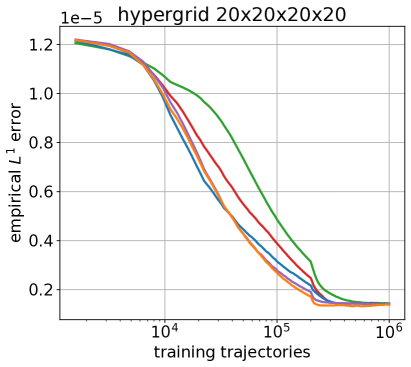
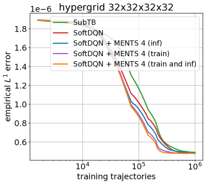
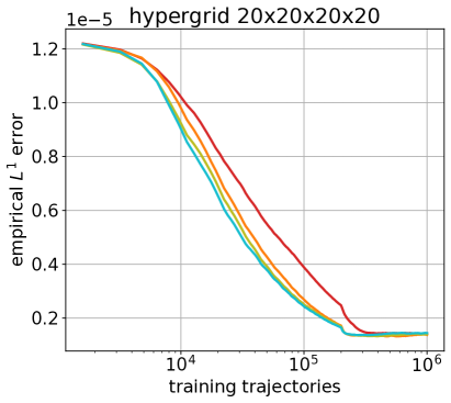
We study 3 setups: 1) a model is trained with vanilla SoftDQN and evaluated with MENTS; 2) a model is trained with MENTS targets, but the trained policy is evaluated without MCTS; 3) MENTS is applied for both training and evaluation. In contrast to (Tiapkin et al., 2024), we do not use replay buffers for training, instead optimizing the loss across trajectories sampled from the current model. As a metric we use distance between the true reward distribution ( can be computed exactly since environments are small) and an empirical distribution of GFlowNet samples.
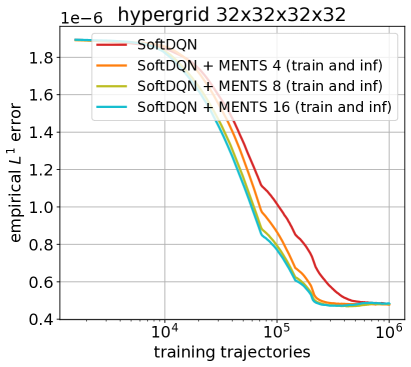
Figure 1 presents the results. We can see that in all setups MENTS offers a stable improvement to the speed of convergence in comparison to vanilla SoftDQN in terms of number of sampled trajectories, which coincides with the number of calls to . The best results are obtained when MENTS is applied for both training and inference of the model. Remarkably, using MENTS to compute targets for the training of provides a noticeable boost even when the model is evaluated without MCTS (setup number 2). Increasing the number of MCTS rounds is also beneficial.
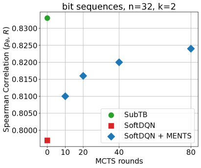

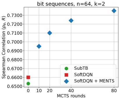
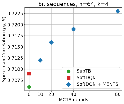
4.2 Bit Sequence Generation
The goal is to generate binary strings of some fixed length . Hyperparameter is introduced, and the string is split into segments of length . Each state corresponds to a sequence of words; each word is either an empty word or one of possible -bit words. corresponds to a sequence of empty words. Possible actions are to take any position with an empty word and replace it with any -bit word. Terminal states contain no empty words and coincide with binary strings of length . , where is a set of modes and is Hamming distance. We use this environment to examine the performance of MCTS in a more challenging setup with larger state and action spaces (up to states and actions in our experiments).
Here we train with SoftDQN paremeterized by Transformer (Vaswani et al., 2017) and utilize MENTS only during inference. Following (Tiapkin et al., 2024) we compute Spearman correlation on a test set of strings between and an estimate of sampling probability . The results are presented in Figure 2. In all configurations, enhancing SoftDQN with MENTS improves the reward correlation in comparison to vanilla SoftDQN, although the improvement is relatively small in some cases. It also outperforms SubTB in 3 out of 4 cases. The metric steadily rises with the increase of the number of MCTS rounds.
5 Conclusion
In this paper, we proposed to apply MENTS (Xiao et al., 2019) algorithm with SoftDQN (Haarnoja et al., 2017) to GFlowNet training and inference. Our experimental results demonstrated the benefits of incorporating MCTS planning for amortized sampling, suggesting new research directions. Future work could explore other MCTS-type approaches, validate them in other domains, and apply MCTS on top of other GFlowNet algorithms, e.g. SubTB (Madan et al., 2023).
Acknowledgements
The work of Nikita Morozov, Sergey Samsonov and Alexey Naumov was supported by the grant for research centers in the field of AI provided by the Analytical Center for the Government of the Russian Federation (ACRF) in accordance with the agreement on the provision of subsidies (identifier of the agreement 000000D730321P5Q0002) and the agreement with HSE University No. 70-2021-00139. The work of Daniil Tiapkin was supported by the Paris Île-de-France Région in the framework of DIM AI4IDF. This research was supported in part through computational resources of HPC facilities at HSE University (Kostenetskiy et al., 2021).
References
- Atanackovic et al. (2024) Atanackovic, L., Tong, A., Wang, B., Lee, L. J., Bengio, Y., and Hartford, J. S. Dyngfn: Towards bayesian inference of gene regulatory networks with gflownets. Advances in Neural Information Processing Systems, 36, 2024.
- Bengio et al. (2021) Bengio, E., Jain, M., Korablyov, M., Precup, D., and Bengio, Y. Flow network based generative models for non-iterative diverse candidate generation. Advances in Neural Information Processing Systems, 34:27381–27394, 2021.
- Bengio et al. (2023) Bengio, Y., Lahlou, S., Deleu, T., Hu, E. J., Tiwari, M., and Bengio, E. Gflownet foundations. Journal of Machine Learning Research, 24(210):1–55, 2023.
- Chen & Mauch (2023) Chen, Y. and Mauch, L. Order-preserving gflownets. In The Twelfth International Conference on Learning Representations, 2023.
- Coulom (2006) Coulom, R. Efficient selectivity and backup operators in monte-carlo tree search. In International conference on computers and games, pp. 72–83. Springer, 2006.
- Deleu et al. (2024) Deleu, T., Nouri, P., Malkin, N., Precup, D., and Bengio, Y. Discrete probabilistic inference as control in multi-path environments. arXiv preprint arXiv:2402.10309, 2024.
- Geist et al. (2019) Geist, M., Scherrer, B., and Pietquin, O. A theory of regularized markov decision processes. In International Conference on Machine Learning, pp. 2160–2169. PMLR, 2019.
- Haarnoja et al. (2017) Haarnoja, T., Tang, H., Abbeel, P., and Levine, S. Reinforcement learning with deep energy-based policies. In International conference on machine learning, pp. 1352–1361. PMLR, 2017.
- Haarnoja et al. (2018) Haarnoja, T., Zhou, A., Abbeel, P., and Levine, S. Soft actor-critic: Off-policy maximum entropy deep reinforcement learning with a stochastic actor. In International conference on machine learning, pp. 1861–1870. PMLR, 2018.
- Hu et al. (2023) Hu, E. J., Jain, M., Elmoznino, E., Kaddar, Y., Lajoie, G., Bengio, Y., and Malkin, N. Amortizing intractable inference in large language models. In The Twelfth International Conference on Learning Representations, 2023.
- Jain et al. (2022) Jain, M., Bengio, E., Hernandez-Garcia, A., Rector-Brooks, J., Dossou, B. F., Ekbote, C. A., Fu, J., Zhang, T., Kilgour, M., Zhang, D., et al. Biological sequence design with gflownets. In International Conference on Machine Learning, pp. 9786–9801. PMLR, 2022.
- Jain et al. (2023) Jain, M., Deleu, T., Hartford, J., Liu, C.-H., Hernandez-Garcia, A., and Bengio, Y. Gflownets for ai-driven scientific discovery. Digital Discovery, 2(3):557–577, 2023.
- Kocsis & Szepesvári (2006) Kocsis, L. and Szepesvári, C. Bandit based monte-carlo planning. In European conference on machine learning, pp. 282–293. Springer, 2006.
- Kostenetskiy et al. (2021) Kostenetskiy, P., Chulkevich, R., and Kozyrev, V. Hpc resources of the higher school of economics. In Journal of Physics: Conference Series, volume 1740, pp. 012050. IOP Publishing, 2021.
- Madan et al. (2023) Madan, K., Rector-Brooks, J., Korablyov, M., Bengio, E., Jain, M., Nica, A. C., Bosc, T., Bengio, Y., and Malkin, N. Learning gflownets from partial episodes for improved convergence and stability. In International Conference on Machine Learning, pp. 23467–23483. PMLR, 2023.
- Malkin et al. (2022) Malkin, N., Jain, M., Bengio, E., Sun, C., and Bengio, Y. Trajectory balance: Improved credit assignment in gflownets. Advances in Neural Information Processing Systems, 35:5955–5967, 2022.
- Mnih et al. (2015) Mnih, V., Kavukcuoglu, K., Silver, D., Rusu, A. A., Veness, J., Bellemare, M. G., Graves, A., Riedmiller, M., Fidjeland, A. K., Ostrovski, G., et al. Human-level control through deep reinforcement learning. nature, 518(7540):529–533, 2015.
- Mohammadpour et al. (2024) Mohammadpour, S., Bengio, E., Frejinger, E., and Bacon, P.-L. Maximum entropy gflownets with soft q-learning. In International Conference on Artificial Intelligence and Statistics, pp. 2593–2601. PMLR, 2024.
- Neu et al. (2017) Neu, G., Jonsson, A., and Gómez, V. A unified view of entropy-regularized markov decision processes. arXiv preprint arXiv:1705.07798, 2017.
- Paszke et al. (2019) Paszke, A., Gross, S., Massa, F., Lerer, A., Bradbury, J., Chanan, G., Killeen, T., Lin, Z., Gimelshein, N., Antiga, L., et al. Pytorch: An imperative style, high-performance deep learning library. Advances in neural information processing systems, 32, 2019.
- Schaul et al. (2016) Schaul, T., Quan, J., Antonoglou, I., and Silver, D. Prioritized experience replay. In Bengio, Y. and LeCun, Y. (eds.), 4th International Conference on Learning Representations, ICLR 2016, San Juan, Puerto Rico, May 2-4, 2016, Conference Track Proceedings, 2016. URL http://arxiv.org/abs/1511.05952.
- Schrittwieser et al. (2020) Schrittwieser, J., Antonoglou, I., Hubert, T., Simonyan, K., Sifre, L., Schmitt, S., Guez, A., Lockhart, E., Hassabis, D., Graepel, T., et al. Mastering atari, go, chess and shogi by planning with a learned model. Nature, 588(7839):604–609, 2020.
- Schulman et al. (2017) Schulman, J., Chen, X., and Abbeel, P. Equivalence between policy gradients and soft q-learning. arXiv preprint arXiv:1704.06440, 2017.
- Silver et al. (2016) Silver, D., Huang, A., Maddison, C. J., Guez, A., Sifre, L., Van Den Driessche, G., Schrittwieser, J., Antonoglou, I., Panneershelvam, V., Lanctot, M., et al. Mastering the game of go with deep neural networks and tree search. nature, 529(7587):484–489, 2016.
- Silver et al. (2018) Silver, D., Hubert, T., Schrittwieser, J., Antonoglou, I., Lai, M., Guez, A., Lanctot, M., Sifre, L., Kumaran, D., Graepel, T., Lillicrap, T., Simonyan, K., and Hassabis, D. A general reinforcement learning algorithm that masters chess, shogi, and go through self-play. Science, 362(6419):1140–1144, 2018. doi: 10.1126/science.aar6404.
- Tiapkin et al. (2024) Tiapkin, D., Morozov, N., Naumov, A., and Vetrov, D. P. Generative flow networks as entropy-regularized rl. In International Conference on Artificial Intelligence and Statistics, pp. 4213–4221. PMLR, 2024.
- Vaswani et al. (2017) Vaswani, A., Shazeer, N., Parmar, N., Uszkoreit, J., Jones, L., Gomez, A. N., Kaiser, Ł., and Polosukhin, I. Attention is all you need. Advances in neural information processing systems, 30, 2017.
- Xiao et al. (2019) Xiao, C., Huang, R., Mei, J., Schuurmans, D., and Müller, M. Maximum entropy monte-carlo planning. Advances in Neural Information Processing Systems, 32, 2019.
- Zhang et al. (2023) Zhang, D., Dai, H., Malkin, N., Courville, A. C., Bengio, Y., and Pan, L. Let the flows tell: Solving graph combinatorial problems with gflownets. In Advances in Neural Information Processing Systems, volume 36, pp. 11952–11969, 2023.
Appendix A Algorithm Details
Algorithm 1 presents a detailed pseudo-code for sampling a trajectory with MENTS applied on top of a GFlowNet pre-trained with SoftDQN.
A.1 Connection to GFlowNet State and Edge Flows
Suppose we have forward and backward policies that satisfy trajectory balance constraints (1). Then, we have a fixed distribution over complete trajectories
| (10) |
GFlowNet literature often operates with flows functions (Bengio et al., 2023). Markovian flow in this case is a function that coincides with unnormalized probability of sampling a trajectory . Since for any fixed and there exists a unique satisfying (1), any fixed and also define a unique Markovian flow. State flows and edge flows are defined as , correspondingly, and coincide with unnormalized probabilities that a trajectory passes through some state/edge.
Flow matching constraint states that for any state that is not or terminal
| (11) |
while for and terminal states, only one of the two equalities holds.
and can be computed in terms of state and edge flows
| (12) |
Let us go back to the RL interpretation. In addition to the optimal policy, Theorem 1 of (Tiapkin et al., 2024) connects state and edge flows with optimal entropy-regularized values and Q-values, stating
| (13) |
In this interpretation, (3) transforms into
| (14) | ||||
which can also be obtained from (12). The equation on the optimal policy transforms into
| (15) |
which also coincides with the equation on from (12).
Appendix B Experimental Details
We utilize PyTorch (Paszke et al., 2019), and our implementations are based upon the published code of (Tiapkin et al., 2024). We implement MENTS in C++ for better performance.
B.1 Hypergrid
The reward at a terminal state with coordinates is defined as
We use similar hyperparameters to previous works (Bengio et al., 2021; Malkin et al., 2022; Madan et al., 2023; Tiapkin et al., 2024). All models are parameterized by MLP with 2 hidden layers and 256 hidden units. We use Adam optimizer with a learning rate of and a batch size of 16 trajectories. We take SubTB hyperparameter . The difference from (Tiapkin et al., 2024) is that for SoftDQN, we do not use a replay buffer and use MSE loss instead of Huber. We use hard updates for the target network (Mnih et al., 2015) with a frequency of iterations. For MENTS we take . We perform hypergrid experiments on CPUs.
In Table 1, we measure the runtime of the algorithms during training and inference. As expected, the speed of MENTS decreases with the increase of the number of rounds due to additional evaluations. However, we note that training with MENTS (4 rounds) runs faster than with SubTB and has better convergence than both SubTB and vanilla SoftDQN (see Figure 1).
| Method | Training | Inference |
|---|---|---|
| SubTB | 8.5 it/s | 35.6 it/s |
| SoftDQN | 20.5 it/s | 35.8 it/s |
| SoftDQN + MENTS 4 | 12.3 it/s | 14.0 it/s |
| SoftDQN + MENTS 8 | 8.1 it/s | 9.2 it/s |
| SoftDQN + MENTS 16 | 5.3 it/s | 6.3 it/s |
B.2 Bit Sequences
The set of modes is constructed as defined in (Malkin et al., 2022), and we use the same size . Take . Then, each sequence in is constructed by randomly taking elements from with replacement and concatenating them. The test set for computing reward correlations is constructed by taking a mode and flipping random bits in it, which is done for each mode and each .
We use the same Monte Carlo estimate for as in (Tiapkin et al., 2024):
All models are parameterized by Transformer (Vaswani et al., 2017) with 2 hidden layers, 8 attention heads and 64 hidden dimension. We use Adam optimizer with a learning rate of and a batch size of . For SubTB we tune from . For training SoftDQN, we use hard updates for the target network with a frequency of iterations and use Huber loss following (Tiapkin et al., 2024). We also utilize a prioritized replay buffer (Schaul et al., 2016) with the same hyperparameters as in (Tiapkin et al., 2024). For MENTS we take . We use NVIDIA A100 GPUs for bit sequence experiments.
In this case the runtime cost of tree manipulation in MCTS is dominated by the cost of forward passes, thus the inference speed decreases proportionally to the number of MCTS rounds.