Intrinsic Modeling of Shape-Constrained Functional Data, With Applications to Growth Curves and Activity Profiles

Abstract

Shape-constrained functional data encompass a wide array of application fields especially in the life sciences, such as activity profiling, growth curves, healthcare and mortality. Most existing methods for general functional data analysis often ignore that such data are subject to inherent shape constraints, while some specialized techniques rely on strict distributional assumptions. We propose an approach for modeling such data that harnesses the intrinsic geometry of functional trajectories by decomposing them into size and shape components. We focus on the two most prevalent shape constraints, positivity and monotonicity, and develop individual-level estimators for the size and shape components. Furthermore, we demonstrate the applicability of our approach by conducting subsequent analyses involving Fréchet mean and Fréchet regression and establish rates of convergence for the empirical estimators. Illustrative examples include simulations and data applications for activity profiles for Mediterranean fruit flies during their entire lifespan and for data from the Zürich longitudinal growth study.

Keywords: Fréchet regression, functional data analysis, longitudinal studies, monotonicity, positivity, size-shape decomposition.

1 Introduction

Functional data contain sample of time-indexed trajectories are often encountered in the life sciences (Ramsay and Silverman, 2005; Hsing and Eubank, 2015; Wang et al., 2016), where such data may be susceptible to shape constraints, with positivity and monotonicity as the most common constraints. Examples that we will study in this paper include activity profile data and data on human growth and development. But many other functional data such as data on mortality, temperature and biomarkers or longitudinal blood pressure are subject to such constraints. Standard approaches like functional principal component analysis (FPCA) commonly employed for functional data (Kleffe, 1973; Dauxois et al., 1982; Castro et al., 1986; Hall et al., 2006; Chen and Lei, 2015) typically do not respect these constraints, due to the non-linearity of the space of shape-constrained functional data, as for example linear combinations of positive functions are not necessarily positive. Consequently, the estimated trajectories obtained through the Karhunen-Loève decomposition (Karhunen, 1947; Loève, 1978) generally will not reside in the constrained space.

For functional data that are constrained to be positive, a potential remedy is to employ FPCA as a dimension reduction tool on the log-transformed observed data, which are situated in the unconstrained space $L^{2}([0,1])$. Subsequently, we can map the estimates obtained for transformed data to the original space by exponentiating (Ramsay and Silverman, 2005; Petersen and Müller, 2016). However, this transformation approach introduces a transformation bias, which can be challenging to address. An analogous transformation approach can be applied for monotone functional data; see Section 5.

Some noteworthy recent works in shape-constrained regression models impose restrictions on the regression coefficient functions modeled using Bernstein polynomial basis expansions (Ghosal et al., 2023), where again shape restrictions are not directly imposed on the underlying stochastic process. On the other hand, shape-constrained generalized additive models (Pya and Wood, 2015; Chen and Samworth, 2016) impose restrictions on each component of the additive prediction function and derive likelihood-based non-parametric estimators using iterative optimization methods, where likelihood based methods have the downside that they are sensitive to model misspecification.

To address these limitations, we propose a decomposition-based approach for shape-constrained functional data. A related decomposition approach has been used for Cox point process regression models (Gajardo and Müller, 2021). The specific definition and interpretation of the components of the proposed decomposition depends on the nature of the constraint. Generally, the size component represents an overall amplitude feature of the trajectory, while the shape component captures temporal (or age-related) variations. This individual-level size-shape decomposition analysis not only offers flexibility but also explores the intrinsic geometry of functional data, enhancing interpretability. The proposed approach is novel and does not rely on narrow distributional or structural assumptions, making it applicable to all positive or monotone constrained functional data. It is nonparametric, does not involve the use of functional principal components and respects the shape-constraints in the data without introducing data distortion or loss of interpretability. We establish uniform rates of convergence for the proposed estimates, uniform over subjects as well as the time domain. In the presence of covariates, the proposed approach utilizes Fréchet regression (Petersen and Müller, 2019) for the decomposition components and it will be illustrated with data on medfly lifetime activity profiles and data from the Zürich longitudinal growth study.

The rest of the paper is organized as follows. Section 2 introduces the decomposition approach for shape-constrained functional data, which is tied to local and global Fréchet regression for the size-shape decomposition components in Section 3. In Section 4, we introduce the proposed estimates and establish their rates of convergence. Simulation studies and data applications are discussed in Sections 5 and 6 respectively, followed by a brief discussion in Section 7. Proofs, auxiliary results and additional data illustrations are in the Supplement.

2 Modeling Shape-Constrained Functional Data

2.1 Positive functional data

Let $Y:\mathcal{T}\rightarrow\mathcal{S}\subset(0,\infty)$ be a strictly positive-valued stochastic process defined on a compact time domain $\mathcal{T}$. Without loss of generality, we assume $\mathcal{T}=\left[0,1\right]$. Denoting by

$$\Omega=\{Y\in L^{2}([0,1]):\,Y(t)>0,t\in[0,1]\}$$

the space of strictly positive functions, for each $Y\in\Omega$, we consider the decomposition into two components, size and shape, defined as

1. Size component: A scalar $\tau=\int_{0}^{1}Y(t)dt\ .$

2. Shape component: A shape function $f:[0,1]\rightarrow(0,\infty)$, defined as
   $f(t):=\frac{Y(t)}{\tau}$, where $\int_{0}^{1}f(t)dt=1.$

We use the symbols $\Omega_{\mathcal{T}}$ and $\Omega_{\mathcal{F}}$ to represent the space where the size and shape components reside, respectively, where $\Omega_{\mathcal{T}}=\mathbb{R}^{+}$ and $\Omega_{\mathcal{F}}$ is the space of density functions that belong to probability measures on $[0,1]$, which can also be represented in terms of their corresponding quantile functions. Specifically, we use $\mathcal{Q}\left(\Omega_{F}\right)$ to denote the space of quantile functions for $\Omega_{\mathcal{F}}$, where each shape function $f\in\Omega_{\mathcal{F}}$ has a unique associated probability measure $\nu(f)$ that can be quantified in terms of its cumulative distribution function $\nu(F)$ or its quantile function $\nu(Q)$. The decomposition $Y=\tau f$ naturally defines a one-to-one correspondence between $Y$ and $(\tau,f)$ through a $1:1$ map $\Psi:\Omega\rightarrow\Omega_{\mathcal{T}}\times\Omega_{\mathcal{F}}$. Endowing $\Omega_{\mathcal{T}}$ and $\Omega_{\mathcal{F}}$ with metrics $d_{\mathcal{T}}$ and $d_{\mathcal{F}}$, respectively, $(\Omega,d)$ can be regarded as a product metric space $\left(\Omega_{\mathcal{T}},d_{\mathcal{T}}\right)\times\left(\Omega_{\mathcal{F}},d_{\mathcal{F}}\right)$, with metric $d$ defined as

$$d\left(Y_{1},Y_{2}\right)=d\left(\Psi^{-1}\left(\tau_{1},f_{1}\right),\Psi^{-1}\left(\tau_{2},f_{2}\right)\right):=\sqrt{d_{\mathcal{T}}^{2}\left(\tau_{1},\tau_{2}\right)+d_{\mathcal{F}}^{2}\left(f_{1},f_{2}\right)}\ ,Y_{1},Y_{2}\in\Omega.$$ (1)

In some cases one can also consider more general metrics given by $d(Y_{1},Y_{2})=\\ \sqrt{w_{1}\ d_{\mathcal{T}}^{2}\left(\tau_{1},\tau_{2}\right)+w_{2}\ d_{\mathcal{F}}^{2}\left(f_{1},f_{2}\right)}$ with weights $w_{1},w_{2}\geq 0$. The theoretical results in Section 4 can be easily extended to this general case.

We select the Euclidean metric $d_{E}$ as a natural choice for $d_{\mathcal{T}}$ and the 2-Wasserstein metric for $d_{\mathcal{F}}$. While other choices might also be of interest, the Wasserstein metric $d_{W}$ has proved to be useful in practical applications involving samples of distributions (Bolstad et al., 2003; Zhang and Müller, 2011). Let $\nu(f)$, $\nu(Q)$, $\nu(F)$ denote the probability measure associated with a given probability density function $f$, quantile function $Q$, and cumulative distribution function $F$. For two probability measures $\nu_{1}$ and $\nu_{2}$ with quantile functions $Q_{\nu_{1}}$ and $Q_{\nu_{2}}$, the 2-Wasserstein distance for univariate distributions is

$$d_{W}^{2}\left(\nu_{1},\nu_{2}\right)=\int_{0}^{1}\left(Q_{\nu_{1}}(t)-Q_{\nu_{2}}(t)\right)^{2}dt.$$

For any two densities $f_{1},f_{2}\in\Omega_{\mathcal{F}}$, we write $d_{W}^{2}\left(f_{1},f_{2}\right):=d_{W}^{2}\left(\nu(f_{1}),\nu(f_{2})\right)$ and analogously $d_{W}^{2}\left(F_{1},F_{2}\right):=d_{W}^{2}\left(\nu(F_{1}),\nu(F_{2})\right)$ for any two cumulative distribution functions $F_{1}$ and $F_{2}$. The Fréchet mean of $Y$ is defined as $Y_{\oplus}=\underset{\omega\in\Omega}{\operatorname{argmin}}\ V(\omega)$, which denotes the potentially multiple minimizers of the Fréchet function

$$V(\omega):=\mathbb{E}\left(d^{2}\left(Y,\omega\right)\right)=\mathbb{E}\left(d_{E}^{2}\left(\tau,\tau(\omega)\right)\right)+\mathbb{E}\left(d_{W}^{2}\left(f,f(\omega)\right)\right),$$

where $\left(\tau(\omega),f(\omega)\right)=\Psi\left(\omega\right)$ and $(\tau,f)=\Psi\left(Y\right)$. Thus,

$$\Psi\left(Y_{\oplus}\right)=\underset{\tau(\omega)\in\Omega_{\mathcal{T}},f(\omega)\in\Omega_{\mathcal{F}}}{\operatorname{argmin}}\left(\mathbb{E}\left[d_{E}^{2}\left(\tau,\tau(\omega)\right)\right]+\mathbb{E}\left[d_{W}^{2}\left(f,f(\omega)\right)\right]\right)=\left(\tau_{\oplus},f_{\oplus}\right),$$

where $\tau_{\oplus}=\underset{\tau(\omega)\in\Omega_{\mathcal{T}}}{\operatorname{argmin}}\ \mathbb{E}\left(d_{E}^{2}\left(\tau,\tau(\omega)\right)\right)$ and $f_{\oplus}=\underset{f(\omega)\in\Omega_{\mathcal{F}}}{\operatorname{argmin}}\ \mathbb{E}\left(d_{W}^{2}\left(f,f(\omega)\right)\right)$ is the density corresponding to the quantile function $Q_{\oplus}=\underset{Q(\omega)\in{\mathcal{Q}}\left(\Omega_{\mathcal{F}}\right)}{\operatorname{argmin}}\mathbb{E}\left(d_{L^{2}}^{2}\left(Q,Q(\omega)\right)\right)$. The optimization problem is thus separable and has a unique solution $Y_{\oplus}=\Psi^{-1}\left(\left(\tau_{\oplus},f_{\oplus}\right)\right)=\tau_{\oplus}\cdot f_{\oplus}.$

2.2 Monotone functional data

Let $Y:[0,1]\rightarrow\mathcal{R}$ be a stochastic process with smooth and srictly monotone increasing (non-constant) trajectories. We write $\Omega\subset L^{2}([0,1])$ to denote the corresponding function space. We focus here on monotone increasing functional data and our considerations apply analogously to processes with monotone decreasing trajectories. We decompose each monotone trajectory $Y\in\Omega$ into

1. Size component: A two-dimensional vector $\xi=\left(\rho,\lambda\right)$ denoting the range and the minimum value of the monotone function, with $\rho=Y(1)-Y(0)>0\ \text{and }\ \lambda=Y(0).$

2. Shape component: A cumulative distribution function $F:[0,1]\rightarrow[0,1]$, defined as $F(t):=\left(Y(t)-Y(0)\right)/\rho\ .$

With similar notations as in the case of positive functions, $Y=\lambda+\rho F$ defines a correspondence between $Y$ and $(\xi,F)=(\rho,\lambda,F)$ through the $1:1$ map $\Psi:\Omega\rightarrow\Omega_{\mathcal{T}}\times\Omega_{\mathcal{F}}$. Again, if we endow spaces $\Omega_{\mathcal{T}}$ and $\Omega_{\mathcal{F}}$ with metrics $d_{\mathcal{T}}$ and $d_{\mathcal{F}}$ respectively, $(\Omega,d)$ can be regarded as a product metric space $\left(\Omega_{\mathcal{T}},d_{\mathcal{T}}\right)\times\left(\Omega_{\mathcal{F}},d_{\mathcal{F}}\right)$. With metric choices $d_{\mathcal{T}}\left(\xi_{1},\xi_{2}\right):=d_{E}\left(\xi_{1},\xi_{2}\right)=\sqrt{(\rho_{1}-\rho_{2})^{2}+(\lambda_{1}-\lambda_{2})^{2}}$ for $\xi_{1},\xi_{2}\in\Omega_{\mathcal{T}}$ and $d_{\mathcal{F}}\left(F_{1},F_{2}\right):=d_{\mathbb{L}^{2}\left(\left[0,1\right]\right)}\left(Q_{1},Q_{2}\right)=d_{W}\left(\nu(F_{1}),\nu(F_{2})\right)$, the metric $d$ in $\Omega$ as

$$d\left(Y_{1},Y_{2}\right)=\sqrt{d_{E}^{2}\left(\xi_{1},\xi_{2}\right)+d_{W}^{2}\left(F_{1},F_{2}\right)}=\sqrt{(\rho_{1}-\rho_{2})^{2}+(\lambda_{1}-\lambda_{2})^{2}+d^{2}_{\mathbb{L}^{2}\left(\left[0,1\right]\right)}\left(Q_{1},Q_{2}\right)}.$$ (2)

Fréchet means are $\xi_{\oplus}=\underset{\xi(\omega)\in\Omega_{\mathcal{T}}}{\operatorname{argmin}}\ \mathbb{E}\left(d_{E}^{2}\left(\xi,\xi(\omega)\right)\right):=\left(\rho_{\oplus},\lambda_{\oplus}\right)$ and
$F_{\oplus}=\underset{F(\omega)\in\Omega_{\mathcal{F}}}{\operatorname{argmin}}\ \mathbb{E}\left(d_{W}^{2}\right.$ $\left.\left(F,F(\omega)\right)\right)$, with $Q_{\oplus}=F^{-1}_{\oplus}=\underset{Q(\omega)\in{\mathcal{Q}}\left(\Omega_{\mathcal{F}}\right)}{\operatorname{argmin}}\mathbb{E}\left(d_{L^{2}}^{2}\left(Q,Q(\omega)\right)\right)$.
Combining these minimizers, we obtain $Y_{\oplus}=\lambda_{\oplus}+\rho_{\oplus}\cdot F_{\oplus}$.

3 Functional regression under shape-constraints

We now extend our discussion beyond Fréchet means and regress the decomposition components on Euclidean predictors. Considering positive functional data, the local Fréchet regression function of $Y$ on $X\in\mathcal{X}\subset\mathcal{R}^{p}$ is

$$Y_{\oplus}(x)=\underset{Y_{0}\in\Omega}{\operatorname{argmin}}\ \mathbb{E}\left(d^{2}\left(Y,Y_{0}\right)\mid X=x\right) =\underset{(\tau_{0},f_{0})\in\Omega_{\mathcal{T}}\times\Omega_{\mathcal{F}}}{\operatorname{argmin}}\mathbb{E}\left(d_{E}^{2}\left(\tau,\tau_{0}\right)+d_{W}^{2}\left(f,f_{0}\right)\mid X=x\right)$$

$$=\Psi^{-1}(\tau_{\oplus}(x),f_{\oplus}(x))=\tau_{\oplus}(x)\cdot f_{\oplus}(x),$$ (3)

where $\tau_{\oplus}(x)$ and $f_{\oplus}(x)$ are defined as

$$\tau_{\oplus}(x) =\underset{\tau_{0}\in\Omega_{\tau}}{\operatorname{argmin}}\ \mathbb{E}\left[d_{E}^{2}\left(\tau,\tau_{0}\right)\mid X=x\right]=\mathbb{E}\left[\tau\mid X=x\right]\text{ and }$$

$$f_{\oplus}(x) =\underset{f_{0}\in\Omega_{F}}{\operatorname{argmin}}\ \mathbb{E}\left[d_{W}^{2}\left(f,f_{0}\right)\mid X=x\right],$$ (4)

Extending this approach to monotone functional data, analogous to $\tau_{\oplus}(x)$ in (3), define $\xi_{\oplus}(x)=\left(\rho_{\oplus}(x),\lambda_{\oplus}(x)\right)$ where $\rho_{\oplus}(x)=\mathbb{E}\left[\rho\mid X=x\right]$ and $\lambda_{\oplus}(x)=\mathbb{E}\left[\lambda\mid X=x\right]$. Analogous to $f_{\oplus}(x)$ in (3), the localized Fréchet mean for shape is

$$F_{\oplus}(x)=\underset{F(\omega)\in\Omega_{F}}{\operatorname{argmin}}\ \mathbb{E}\left(d_{W}^{2}\left(F,F(\omega)\right)\mid X=x\right)$$

and can alternatively be obtained through quantile function representations

$$Q_{\oplus}(x)=F^{-1}_{\oplus}(x)=\underset{Q(\omega)\in\mathcal{Q}\left(\Omega_{F}\right)}{\operatorname{argmin}}\mathbb{E}\left(d_{L^{2}([0,1])}^{2}\left(Q,Q(\omega)\right)\mid X=x\right).$$

Using $Y=\lambda+\rho F$ in (2),

$$Y_{\oplus}(x)=\lambda_{\oplus}(x)+\rho_{\oplus}(x)F_{\oplus}(x).$$ (5)

To facilitate inclusion of categorical predictors into our model, we use a global Fréchet regression function $Y_{\mathrm{G_{\oplus}}}(x):=\underset{w\in\Omega}{\operatorname{argmin}}\ \mathbb{E}\left(s(X,x)\ d^{2}(Y,w)\right),\text{with}\ s(X,x):=1+(X-\mu)^{T}\Sigma^{-1}(x-\mu)$. We assume $\mu:=\mathbb{E}(X)$ and $\Sigma:=\operatorname{Var}(X)$ exist, with positive definite $\Sigma$. The key idea involves characterization of multiple linear regression as a weighted sum of the responses, which can then be generalized to the case of weighted Fréchet means (Petersen and Müller, 2019), wherein the global weights $s(X,x)$ do not depend on tuning parameters, unlike local methods. Using metric decomposition for positive functional $Y$,

$$Y_{\mathrm{G_{\oplus}}}(x)=\tau_{\mathrm{G_{\oplus}}}(x)\cdot f_{\mathrm{G_{\oplus}}}(x),\text{ where }\tau_{\mathrm{G_{\oplus}}}(x)=\underset{\tau_{0}\in\Omega_{\mathcal{T}}}{\operatorname{argmin}}\ \mathbb{E}\left(s(X,x)\ d_{E}^{2}\left(\tau,\tau_{0}\right)\right)\text{ and }$$

$$f_{\mathrm{G_{\oplus}}}(x)=\underset{f_{0}\in\Omega_{\mathcal{F}}}{\operatorname{argmin}}\ \mathbb{E}\left(s(X,x)\ d_{W}^{2}\left(f,f_{0}\right)\right).$$ (6)

Analogous to $\tau_{\mathrm{G_{\oplus}}}(x)$ in (3) for monotone functional data,

$$\xi_{G_{\oplus}}(x)=\underset{\xi_{0}\in\Omega_{\mathcal{T}}\subset\mathcal{R}^{2}}{\operatorname{argmin}}\ \mathbb{E}\left(s(X,x)\ d_{E}^{2}\left(\xi,\xi_{0}\right)\right)\newline =\left(\rho_{G_{\oplus}}(x),\lambda_{G_{\oplus}}(x)\right).$$

For shape, ${F}_{G_{\oplus}}(x)=\underset{F(\omega)\in\Omega_{\mathcal{F}}}{\operatorname{argmin}}\ \mathbb{E}(s(X,x)\ d_{W}^{2}(F,F(\omega))$ with

$${Q}_{G_{\oplus}}(\cdot,x)={F}^{-1}_{G_{\oplus}}(x)=\underset{Q(\omega)\in\mathcal{Q}\left(\Omega_{F}\right)}{\operatorname{argmin}}\mathbb{E}\left(s(X,x)\ d_{L^{2}([0,1])}^{2}\left(Q,Q(\omega)\right)\right).$$

Using $Y=\lambda+\rho F$ in (2), the final representation of the fitted monotone function, regressed on the predictor level $X$, is as follows,

$$Y_{G_{\oplus}}(x)=\lambda_{G_{\oplus}}(x)+\rho_{G_{\oplus}}(x)F_{G_{\oplus}}(x).$$ (7)

4 Estimation and Convergence

4.1 Recovery of individual trajectories

Recall that $Y:\mathcal{T}\rightarrow\mathcal{S}$ are the underlying smooth random trajectories. We observe $n$ data trajectories $\left\{Z_{i}\right\}_{i=1}^{n}$ at $N_{i}$ equidistant time points $\{t_{ij}\}_{j=1}^{N_{i}}$ and assume that the available measurements are noisy. The data model is then $Z_{ij}=Z_{i}\left(t_{ij}\right)=Y_{i}\left(t_{ij}\right)+\varepsilon_{ij}$, $j=1,\dots,N_{i}$. A first step is to recover the individual-level true (unobserved) trajectories $Y_{i}$ nonparametrically as follows. We divide $\mathcal{T}=\left[0,1\right]$ into $L$ bins of equal width. To establish a uniform rate of convergence over all the subjects, we use a common bin size $\gamma$, resulting in $\ell=\gamma^{-1}$ bins $\left\{B_{\ell}\right\}_{\ell=1}^{L}$, where $B_{\ell}=[(\ell-1)\gamma,\ell\gamma]$. Then the underlying trajectory $Y_{i}$ is estimated by

$$\widehat{Y}_{i}(t)=\frac{\sum_{j=1}^{N_{i}}\ Z_{ij}\mathds{1}_{\{t_{ij}\in B_{\ell}\}}}{\sum_{j=1}^{N_{i}}\ \mathds{1}_{\{t_{ij}\in B_{\ell}\}}},\ \text{for}\ t\in B_{\ell}.$$ (8)

To establish rates of convergence, we require a few additional assumptions.

1. The measurement noise $\varepsilon$ is independent of the underlying stochastic process $Y$. We assume $\varepsilon_{ij}\stackrel{{\scriptstyle\text{i.i.d.}}}{{\sim}}\varepsilon$ with $E(\varepsilon)=0$ and $\text{var}(\varepsilon)=\sigma^{2}<\infty$.

2. There exists a sequence of positive integers $N:=N(n)$ such that $N<\underset{1\leq i\leq n}{\inf}N_{i}$ and $\log n\big{/}N\rightarrow 0$ as $n\rightarrow\infty$.

3. $Y(t)$ is twice continuously differentiable and there exist real constants $c_{1},c_{2}>0$ such that $\left|Y^{{}^{\prime}}(0)\right|\leq c_{1}$ and ${\sup}_{t\in[0,1]}\ \left|Y^{{}^{\prime\prime}}(t)\right|\leq c_{2}$ with probability 1.

Assumption (A1) is a standard assumption when functional data are measured with noise. Assumption (A2) provides a uniform lower bound on the number of observations for each subject, which is necessary to obtain rates uniform over subjects. Assumption (A3) imposes a smoothness constraint on the trajectories. With these assumptions in place, we obtain a rate of convergence $O_{p}\left(\left(\log n\big{/}N\right)^{1/3}\right)$, where this rate is uniform over both all subjects and also the time domain (see the Supplement for details).

4.2 Estimation and theory

We use the individual level estimated trajectories defined in (8) to obtain the following estimates of the latent shape and size components for positive functional data,

$$\widehat{\tau}_{i}:=\frac{1}{N}\sum_{j=1}^{N}Z_{ij}\quad\text{and}\quad\widehat{f}_{i}(t):=\frac{\widehat{Y}_{i}(t)}{\int_{0}^{1}\widehat{Y}_{i}(t)dt},\quad\text{ for all }t\in[0,1]\quad\text{and each }i.$$ (9)

We additionally require assumption (S0) below to ensure that the trajectories are bounded away from zero, to guarantee that the shape estimates well-defined.

1. There exist constants $\kappa_{0},\kappa_{1}>0$ such that realizations of the underlying stochastic process $Y$ satisfy $0<\kappa_{0}\leq\inf_{t\in[0,1]}{Y(t)}\leq\sup_{t\in[0,1]}{Y(t)}\leq\kappa_{1}<\infty$.

Theorem 1.

Under (A1)$-$(A3) the size estimates $\widehat{\tau}_{i}$ defined in (9) satisfy

$$n^{-1}\sum_{i=1}^{n}\ \left|\widehat{\tau}_{i}-\tau_{i}\right|=O_{p}\left(N^{-1/2}\right)\text{ and }\sup_{1\leq i\leq n}\ \left|\widehat{\tau}_{i}-\tau_{i}\right|=O_{p}\left(\left(\log n\big{/}N\right)^{1/2}\right).$$

Under (S0), with bin sizes $\gamma\sim\left(\log n\big{/}N\right)^{1/3}$, the shape estimates $\widehat{f}_{i}(t)$ in (9) satisfy

$$\sup_{1\leq i\leq n}\ \sup_{t\in[0,1]}\ \left|\widehat{f}_{i}(t)-f_{i}(t)\right|=O_{p}\left(\left(\log n\big{/}N\right)^{1/3}\right)\,\,\text{and}\,\,\sup_{1\leq i\leq n}\ d_{W}\left(\widehat{f}_{i},f_{i}\right)=O_{p}\left(\left(\log n\big{/}N\right)^{1/6}\right).$$

The first part of Theorem 1 provides convergence rates for the size components, both on average and uniformly over subjects. The second part illustrates individual-level (uniform) convergence for the shape components, again uniformly over subjects.

Concerning estimation of the corresponding Fréchet means defined in Section 2.1, $\tau_{\oplus}$ is unique by definition and Lemma 1 (see Supplement) guarantees the unique existence of $f_{\oplus}$. Therefore, the minimizer $Y_{\oplus}$ exists uniquely. The estimate for $\tau_{\oplus}$ is given by $\widehat{\tau}_{\oplus}=n^{-1}\sum_{i=1}^{n}\widehat{\tau}_{i}$ and $f_{\oplus}$ is estimated by the density $\widehat{f}_{\oplus}$, corresponding to the quantile function $\widehat{Q}_{\oplus}=\underset{q\in{\mathcal{Q}}\left(\Omega_{\mathcal{F}}\right)}{\operatorname{argmin}}\ \left\|q-n^{-1}\sum_{i=1}^{n}\widehat{Q}_{i}\right\|_{L^{2}([0,1])}^{2}$.

Corollary 1.

Under assumptions (A1)$-$(A3), $\left|\widehat{\tau}_{\oplus}-\tau_{\oplus}\right|=O_{p}\left({N}^{-1/2}+n^{-1/2}\right).$ Under (S0), with $\gamma\sim\left(\log n\big{/}N\right)^{1/3}$, furthermore $d_{W}\left(f_{\oplus},\widehat{f}_{\oplus}\right)=O_{p}\left(\left(\log n\big{/}N\right)^{1/6}+n^{-1/2}\right),$ so that

$$d\left(Y_{\oplus},\widehat{Y}_{\oplus}\right)=O_{p}\left(\left(\log n\big{/}N\right)^{1/6}+n^{-1/2}\right).$$

To facilitate the inclusion of categorical predictors in the regression model, we primarily focus on estimating the global Fréchet regression functions $\tau_{G_{\oplus}}(x)$ and $f_{G_{\oplus}}(x)$. We obtain regression estimates adopting the empirical global weights in Petersen and Müller (2019), defined as $s_{in}(x):=1+\left(X_{i}-\bar{X}\right)^{T}\hat{\Sigma}^{-1}(x-\bar{X})$, where $\bar{X}:=n^{-1}\sum_{i=1}^{n}X_{i}$ and $\hat{\Sigma}:=n^{-1}\sum_{i=1}^{n}\left(X_{i}-\bar{X}\right)\left(X_{i}-\bar{X}\right)^{T}$. The resulting estimate for the scalar size factor $\tau_{G_{\oplus}}(x)$ is the usual least squares estimator $\widehat{\tau}_{G_{\oplus}}(x)=\operatorname{max}\{\kappa_{0},\frac{1}{n}\sum_{i=1}^{n}s_{in}(x)\widehat{\tau}_{i}\}$, constrained to be positive. To obtain the resulting regression for the shape function on Euclidean predictors, we use quantile functions $Q_{i}$ and $\widehat{Q}_{i}$ of $f_{i}$ and $\widehat{f}_{i}$. Deploying empirical global weights $s_{in}(x)$ then leads to the global Fréchet regression estimator

$$\widehat{Q}_{G_{\oplus}}(\cdot,x)=\underset{Q_{0}\in\mathcal{Q}\left(\Omega_{F}\right)}{\operatorname{argmin}}\hskip 5.69054pt\left\|Q_{0}-\frac{1}{n}\sum_{i=1}^{n}s_{in}(x)\widehat{Q}_{i}\right\|^{2}_{L^{2}([0,1])},$$ (10)

with corresponding density function $\widehat{f}_{G_{\oplus}}(x)$. Then (3) leads to the final estimate $\widehat{Y}_{G_{\oplus}}(x)=\widehat{f}_{G_{\oplus}}(x)\cdot\widehat{\tau}_{G_{\oplus}}(x)$ of $Y_{G_{\oplus}}(x)$.

Theorem 2.

Under assumptions (A1)$-$(A3), it holds that

$$\left|\tau_{G_{\oplus}}(x)-\widehat{\tau}_{G_{\oplus}}(x)\right|=O_{p}\left(N^{-1/2}+n^{-1/2}\right).$$ (11)

Additionally under assumption (S0) and with bin size $\gamma\sim\left(\log n\big{/}N\right)^{1/3}$,

$$d_{W}\left(f_{G_{\oplus}}(x),\widehat{f}_{G_{\oplus}}(x)\right)=O_{p}\left(\left(\log n\big{/}N\right)^{1/6}+n^{-1/2}\right).$$ (12)

Using Theorem 2, it is easy to see that $\widehat{Y}_{G_{\oplus}}$ enjoys the same convergence rate as $\widehat{f}_{G_{\oplus}}$.

The remainder of this section pertains to monotone functional data. Based on $\widehat{Y}_{i}$, the individual level estimates for size and shape components are

$$\widehat{\xi}_{i}:=\left(\widehat{\rho}_{i},\widehat{\lambda}_{i}\right)=\left(\widehat{Y}_{i}(1)-\widehat{Y}_{i}(0),\widehat{Y}_{i}(0)\right)\quad\text{and}\quad\widehat{F}_{i}(t):=\frac{\widehat{Y}_{i}(t)-\widehat{Y}_{i}(0)}{\widehat{Y}_{i}(1)-\widehat{Y}_{i}(0)},\quad\text{for all }t\in[0,1].$$ (13)

Under suitable assumptions, one can establish uniform rates of convergence for the decomposition components associated with monotone trajectories, similar to the case of positive trajectories. For the size component $\xi$, one can obtain a $O_{p}\left(\left(\log n\big{/}N\right)^{1/3}\right)$ (uniform) convergence rate and for the shape component $F$ the same convergence rate as for the case of positive trajectories. Following arguments similar to positive functional data, we then obtain convergence rates for Fréchet means and Fréchet regression functions. The results are provided in the Supplement (Section 8.3).

5 Simulation Study

We demonstrate the applicability of our proposed method in recovering the latent decomposition components through simulation studies conducted in a number of setups. To generate positive functional trajectories, we adopt a model that adheres to the positivity constraint. We simulate the sample path $Y_{i}$ on a regular time grid $\{t_{ij}\}_{j=1}^{N}\subset\mathcal{T}$, for $i=1,2,\dots,n$. The underlying trajectory is modeled as $Y_{ij}:=Y_{i}(t_{ij})=\tau_{i}\cdot f_{i}(t_{ij})$, where the shape component $f_{i}$ denotes the density of $\mathcal{N}(\mu_{i},\sigma^{2})$ truncated on time interval $\mathcal{T}$, the size component $\tau_{i}\stackrel{{\scriptstyle\text{i.i.d.}}}{{\sim}}\mathcal{U}(a_{\tau},b_{\tau})$, and $\mu_{i}\stackrel{{\scriptstyle\text{i.i.d.}}}{{\sim}}\mathcal{U}(a_{\mu},b_{\mu})$. We use $a_{\tau}>0$ to ensure the positivity constraint of the underlying trajectories. A similar approach is used for simulating monotone functional data. Instead of $\tau_{i}$, we now generate the size component $\xi_{i}=(\rho_{i},\lambda_{i})$ with $\rho_{i}\stackrel{{\scriptstyle\text{i.i.d.}}}{{\sim}}\mathcal{U}(a_{\rho},b_{\rho})$ and $\lambda_{i}\stackrel{{\scriptstyle\text{i.i.d.}}}{{\sim}}\mathcal{U}(a_{\lambda},b_{\lambda})$. We then simulate the sample path $Y_{i}$ at $\{t_{ij}\}_{j=1}^{N}$ as $Y_{ij}:=Y_{i}(t_{ij})=\rho_{i}\cdot F_{i}(t_{ij})+\lambda_{i}$, where the shape component $F_{i}$ is the cumulative distribution function of $\mathcal{N}(\mu_{i},\sigma^{2})$ truncated on $\mathcal{T}$, which guarantees the monotonicity of the sample path $Y_{i}$. To mimic real-life data and illustrate the effect of noise, we contaminate the true trajectories with white noise $\varepsilon_{ij}\stackrel{{\scriptstyle\text{i.i.d.}}}{{\sim}}\mathcal{N}(0,\nu_{0}^{2})$, resulting in observed values $z_{ij}=Y_{ij}+\varepsilon_{ij}$. Consequently, our simulated dataset on the time domain $\mathcal{T}$ comprises the pairs $(t_{ij},z_{ij})$, where $j=1,\dots,N$ and $i=1,\dots,n$.

We studied the performance of the proposed approach for $N=100,200,500,1000$ observations per subject and noise levels $\nu_{0}=0.05,0.1,0.15$, setting $a_{\tau}=0,b_{\tau}=2,a_{\mu}=0,b_{\mu}=1,\sigma=1,a_{\rho}=0,b_{\rho}=4,a_{\lambda}=-2,b_{\lambda}=2,\text{ and time interval }\mathcal{T}=[0,1]$. For each $(N,\nu_{0})$, the simulation study was performed for $n=500$ independent units and was repeated $B=1000$ times. For the $b$th replicate, the error in estimating the quantity of interest was measured by root-mean-square error (RMSE) based on the corresponding metric defined in Sections 2.1 and 2.2. Note that we are interested in estimating the underlying trajectory, size and shape components. For positive functional data, for the $b$th replicate, ${\text{RMSE}}_{b}^{Y}:={\left(n^{-1}\sum_{i=1}^{n}d^{2}(Y_{i},\widehat{Y_{i}})\right)}^{1/2},\quad\quad{\text{RMSE}}_{b}^{\tau}:={\left(n^{-1}\sum_{i=1}^{n}d_{E}^{2}(\tau_{i},\widehat{\tau_{i}})\right)}^{1/2},\quad\text{and}\\ {\text{RMSE}}_{b}^{f}:={\left(n^{-1}\sum_{i=1}^{n}d_{W}^{2}(f_{i},\widehat{f_{i}})\right)}^{1/2}.$ Analogously, for monotone functional data,
${\text{RMSE}}_{b}^{Y}:={\left(n^{-1}\sum_{i=1}^{n}d^{2}(Y_{i},\widehat{Y_{i}})\right)}^{1/2},\quad\quad{\text{RMSE}}_{b}^{\xi}:={\left(n^{-1}\sum_{i=1}^{n}d_{E}^{2}(\xi_{i},\widehat{\xi_{i}})\right)}^{1/2},\quad\text{and}\\ {\text{RMSE}}_{b}^{F}:={\left(n^{-1}\sum_{i=1}^{n}d_{W}^{2}(F_{i},\widehat{F_{i}})\right)}^{1/2}$.

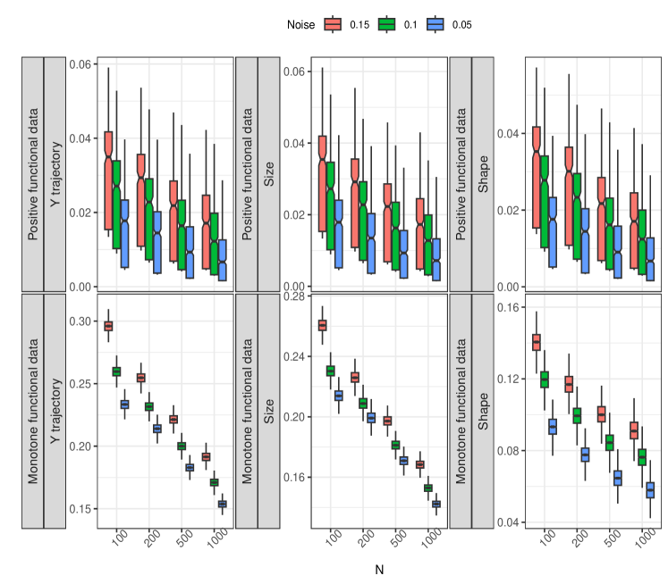
Figure 1: RMSE for the estimation of underlying trajectories $Y_{i}$ with the proposed size-shape decomposition method in dependence on the number of observations $N$ available per subject and the noise variance, both for positive and monotone functional data.

As illustrated in Figure 1, estimation errors are overall quite small and reflect the noise levels; errors decrease as the number of observations per subject increases for a given number of subjects. For positive functional data, the Fréchet mean estimate using the transformation method is $\widehat{\omega}_{\oplus}=\underset{\omega\in\Omega}{\operatorname{argmin}}\ \exp{{n}^{-1}\sum_{i=1}^{n}\left(d^{2}\left(\log Y_{i},\omega\right)\right)}$, and for monotone data it is $\widehat{\omega}_{\oplus}=\underset{\omega\in\Omega}{\operatorname{argmin}}\ \left(\frac{\int_{0}^{t}\exp{{n}^{-1}\sum_{i=1}^{n}\left(d^{2}\left(\log Y_{i}(s),\omega(s)\right)\right)}ds}{\int_{0}^{1}\exp{{n}^{-1}\sum_{i=1}^{n}\left(d^{2}\left(\log Y_{i}(s),\omega(s)\right)\right)}ds}\right)$, with estimation error determined by $d_{L^{2}}\left(Y_{\oplus},\widehat{\omega}_{\oplus}\right)$. For the proposed decomposition method the estimation error is determined by $d_{L^{2}}\left(Y_{\oplus},\widehat{Y}_{\oplus}\right)$, where $Y_{\oplus}$ is the true Fréchet mean. Relative RMSEs are given in Figure 2 and decrease as the number of observation time points increases.

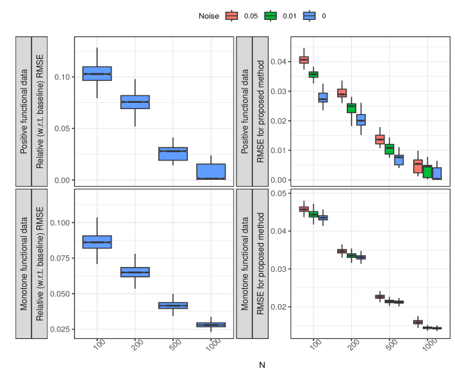
Figure 2: Simulation study for underlying Fréchet mean estimation based on positive and monotone functional data. (Left) Relative RMSE (relative to the transformation approach), for different number of observations ($N$) per subject. (Right) RMSE for different number of observations per subject and varying noise level ($\nu$).

To assess the finite sample performance of global (and local) Fréchet regression estimates, we use the following data generating mechanism for positive functional data. We generate the covariate $X\sim U(0,2)$ and the shape component (density) $f$ corresponds to a truncated normal distribution with support $[0,1]$, mean $\mu(x)=a_{1}+b_{1}x+\varepsilon_{1}$, and standard deviation $\sigma(x)=a_{2}+b_{2}x+\varepsilon_{2}$, where $\varepsilon_{1},\varepsilon_{2}$ are independent (of other random variables too) truncated Normal $(0,\sigma_{0})$ on support $[l_{1},u_{1}]$ and $[l_{2},u_{2}]$ respectively. The size component $\tau=b_{3}x+\varepsilon_{3}$, where $\varepsilon_{3}$ is an i.i.d. copy of $\varepsilon_{2}$. The positive trajectory is thus generated using the decomposition mapping (1). We choose $a_{1}=0.1,b_{1}=0.3,a_{2}=0.1,b_{2}=0.1,b_{3}=0.5,\sigma_{0}=0.5,l_{1}=-0.1,u_{1}=0.1,l_{2}=-0.01,u_{2}=0.01$. A similar generation method is utilized for monotone functional data (see Supplement Section 9.1). Figure 3 shows “oracle” global Fréchet regression functions and their estimated counterparts for one simulation run over a dense grid of predictor values for $n=500$ and $N=500$.

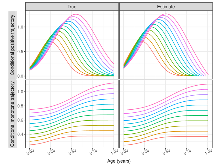
Figure 3: Conditional global Fréchet regression functions in the simulation setting over a dense grid of predictor levels $x$, displayed in red when $x=0.5$ to magenta when $x=1.5$. The left panel displays the “oracle” functions and the right panel illustrates their estimated counterparts, for both positive and monotone functional data.

6 Data Applications

6.1 Medfly Activity Study

The study of patterns of activity across the life sciences has become increasingly popular. We illustrate our method for medfly activity profile data, with a lifetime activity profile available for each of $96$ female Mediterranean fruit flies (medflies). Daily locomotory activity counts were recorded for each medfly until its death (so there is no data censoring) using Monitor-LAM25 systems. The experiment involved three agar-based gel diets C10, C20 and C50 (based on sugar and yeast hydrolysate content: $10\%$, $20\%$ and $50\%$, respectively), each given to $32$ medflies. Further details on the experimental setup can be found in Chen et al. (2024). The activity profiles are positive functional trajectories and the proposed decomposition approach allows us to focus separately on the overall activity count (size component) and the variation of activity over the life cycle (shape component). Age is measured in days, and our Our focus is on flies that survive through a common age window $\left[0,30\right]$ days, where age is measured in days. One goal of the study was to investigate differences between diets and the impact of reproduction, which is quantified through the number of eggs laid by the flies (Chen et al., 2024; Chen et al., 2017).

We first explore the individual-level activity pattern variations in dependence on diet, where Figure 4 shows the distribution of subject-specific size estimates. Median size is seen to increase with higher sugar and protein concentration in diet. Next we use global Fréchet regression model to regress the shape trajectories; to remove boundary effects near age $30$, we use data over a slightly longer age span, where Figure 4 displays conditional shape function estimates.

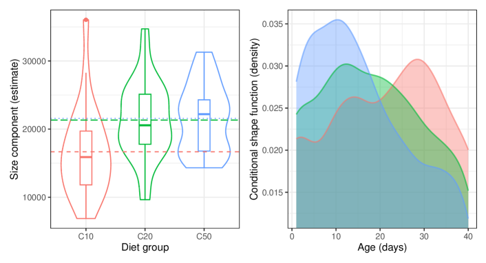
Figure 4: Medfly activity profile study with daily locomotory activity count trajectories viewed as positive functional data. (Left) Distribution of individual-level size estimates, for different diet groups, with horizontal dashed lines representing the respective means. (Right) Conditional shape trajectories obtained for different diet groups using decomposition-based global Fréchet regression model.

To investigate the effects of reproduction on activity, we fit a global Fréchet regression model with shape trajectories as functional responses and total egg counts (obtained over the entire lifespan) as predictors. To illustrate the model, we fit conditional shape functions at five equidistant sample quantiles for total egg counts. Figure 5 highlights that female medflies with higher total egg counts tend to have relatively higher locomotory activity until around age $15$ and lower activity after that. This shows the impact of reproduction on activity; most of the flies begin to lay eggs around age $10$.

Using a similar model to understand the association with lifespan, quantified as age-at-death, we present estimated conditional shape functions for five different quantile levels of age-at-death in Figure 6. For longer lifespans, the shape function tends to have lower initial values, followed by a sharper and higher peak within the age range $[10,20]$, and a sharper decline after that. Including diet as an additional predictor leads to estimated conditional shape components as depicted in Figure 6 for each diet group. Although the overall pattern is similar to that in Figure 5 there is a discernible effect of diet.

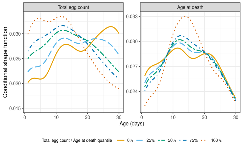
Figure 5: Medfly activity profile study with daily locomotory activity count trajectories viewed as positive functional data. Decomposition-based conditional shape functions across varying quantiles of total egg count and age at death.

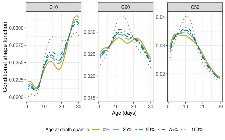
Figure 6: Medfly activity profile study with daily locomotory activity count trajectories viewed as positive functional data. Conditional shape functions across varying quantiles of age at death, and for diet groups with varying glucose-protein concentration, namely, C10 (10$\%$), C20 (20$\%$), and C50 (50$\%$).

6.2 Zürich Longitudinal Study

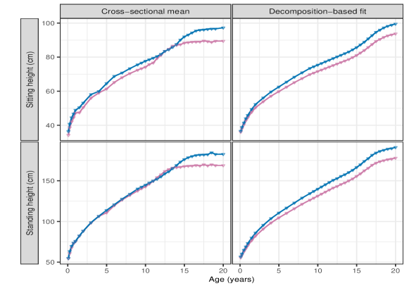
Figure 15: (Top panel) sitting height and (bottom panel) standing height. Cross-sectional mean height trajectories (left) and conditional height trajectories (right) for females (pink) and males (blue), where the latter are obtained using decomposition-based global Fréchet regression model.

A longitudinal study on human growth and development was conducted at the University Children’s Hospital in Zürich from 1954 to 1978. The growth study involved $n=232$ participants comprising $120$ males and $112$ females . Different aspects of growth, including arm length, leg length, sitting height, and standing height, were longitudinally measured at ages 1 month, 3 months, 6 months, 9 months, 1 year, 1.5 years and 2 years; thereafter once every year until age 9 years , and then every 6 months until age 20 years (Bayley and Schaefer, 1964; Ramsay et al., 1995; Chen and Müller, 2012; Carroll et al., 2021). The arm length trajectories correspond to monotone functional data. We fitted a decomposition-based global Fréchet regression model with estimated height trajectories (standing or sitting) as functional responses and sex as predictor, using the estimation approach described in Section 4. The conditional height trajectories illustrate distinct differences in growth patterns with respect to sex, which is not evident in the basic comparison of cross-sectional mean trajectories (See Supplement, Figure 15).

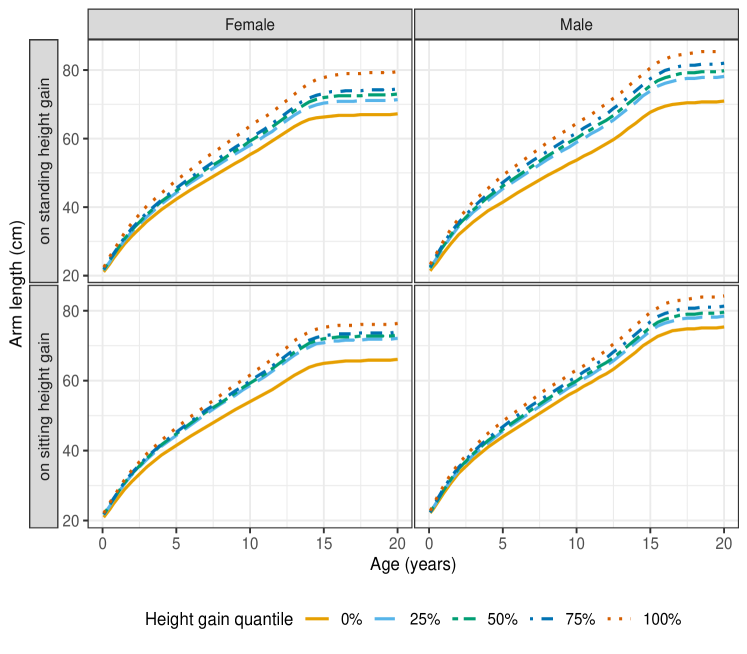
Figure 7: Zürich longitudinal growth study with age-varying arm length trajectories viewed as monotone functional data. Conditional arm length trajectories across varying quantiles of standing (or sitting) height gain for females and males.

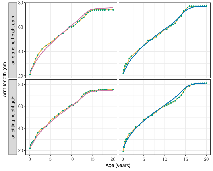
Figure 8: Zürich longitudinal growth study with age-varying arm length trajectories viewed as monotone functional data. Observed arm length measurements (solid green circles, with connecting lines) and predicted arm length trajectories (solid lines) for four randomly selected participants, two females (left) and two males (right). The randomly selected participants are not used in fitting the decomposition-based Fréchet regression model.

We further regress estimated arm length trajectories on standing (or sitting) height gain in the age interval 0 to 20 years. Figure 7 displays conditional arm length trajectories at different sample quantiles of standing (or sitting) height gain for each sex groups. Both the sex groups illustrate a distinct pattern, with expected difference in magnitude between males and females.

To assess model’s predictive accuracy, we randomly select male and female participants. The predicted trajectories for the selected individuals are obtained through a leave-one-out decomposition-based Fréchet regression, using standing (or sitting) height gain as predictor. Note that the randomly selected individuals are not used in model fitting. The predicted arm length trajectories, reported in Figure 8, exhibit a close alignment with the observed arm length measurements.

7 Discussion

In this article, we propose a decomposition-based approach for modeling shape-constrained functional data. Specifically, we decompose functional trajectories into size and shape components, while preserving the inherent constraints, such as positivity and monotonicity, without introducing undesirable data distortions. Importantly, the proposed methodology does not rely on specific distributional or parametric model assumptions, hence offering enhanced applicability. The effectiveness of the proposed decomposition approach is further supported through rates of convergence and simulation studies. The proposed framework also furthers an understanding of the intrinsic geometry of shape-constrained functional data, by separating an overall size feature from the pattern of variation over time or age.

Several other extensions will be of interest for future research. For instance, to further ensure applicability in functional valued stochastic process (Chen et al., 2017), one may extend the proposed decomposition model for modeling functional data subject to other shape restrictions such as convexity or to scenarios with repeated functional data in future research, which may also entail alternative metric choices for the decomposition components.

Funding

This research was supported in part by NSF grants DMS-2014626 and DMS-2310450.

Appendix

8 Additional Results

8.1 Recovery of individual trajectories

The proofs of all additional results are in the Supplement Section LABEL:Proof:Supp. The underlying trajectory $Y_{i}$ for the $i$th subject is estimated by

$$\widehat{Y_{i}}(t)=\frac{\sum_{j=1}^{N_{i}}Z_{ij}\mathds{1}_{\{t_{ij}\in B_{\ell}\}}}{\sum_{j=1}^{N_{i}}\mathds{1}_{\{t_{ij}\in B_{\ell}\}}},\>\text{for}\ t\in B_{\ell}\ \text{and}\ \ell=1,\dots,L,$$

where the $l$th bin $B_{\ell}:=[(\ell-1)\gamma,\ell\gamma]$ with common width $\gamma$.

Theorem 3.

Under assumptions (A1)-(A3) and with $\gamma\sim\left(\log n\big{/}N\right)^{1/3}$,

$$\sup_{1\leq i\leq n}\sup_{t\in[0,1]}\left|\widehat{Y_{i}}(t)-Y_{i}(t)\right|=O_{p}\left((\log n\big{/}N)^{1/3}\right).$$

Note that the rate of convergence $\alpha_{N,n}:=\left(\log n\big{/}N\right)^{1/3}$ in Theorem 3 is uniform over all the subjects and the time domain.

8.2 Estimation and theory for positive functional data

In the local Fréchet regression framework, we use the empirical weights from local linear regression (Fan and Gijbels, 1996), as adopted in Petersen and Müller (2019), where this concept is introduced. The empirical local weights are $s_{in}(x,h)=\widehat{\sigma_{0}}^{-2}K_{h}(X_{i}-x)[\widehat{u}_{2}-\widehat{u}_{1}(X_{i}-x)]$, where $\widehat{u}_{l}=n^{-1}\sum_{i=1}^{n}K_{h}(X_{i}-x)\left(X_{i}-x\right)^{l}$ with $l\in\{0,1,2\},\ \widehat{\sigma}_{0}^{2}=\widehat{u}_{0}\widehat{u}_{2}-\widehat{u}_{1}^{2}$, and $K_{h}(\cdot)=$ $h^{-1}K(\cdot/h)$. Here the kernel $K$ satisfies Assumption (K0) and $h:=h_{n}$ is a sequence of bandwidths.

1. The kernel $K$ is a bounded continuous density function, symmetric around zero.

We further use estimated size $\widehat{\tau}_{i}$ and shape $\widehat{f}_{i}$ as surrogates for the latent (unobservable) decomposition components. For the regression function $\tau_{\oplus}(x)=\arg\min_{\tau_{0}\in\Omega_{\mathcal{T}}=[\kappa_{0},\infty)}\mathbb{E}[(\tau_{0}-\tau)^{2}\mid X=x]$, the intermediate estimate is $\widetilde{\tau}_{\oplus}(x)=\operatorname{max}\{\kappa_{0},n^{-1}\sum_{i=1}^{n}s_{in}(x,h){\tau}_{i}\}$. Replacing $\tau_{i}$ with $\widehat{\tau}_{i}$, the final estimate is $\widehat{\tau}_{\oplus}(x)=\operatorname{max}\{\kappa_{0},n^{-1}\sum_{i=1}^{n}s_{in}(x,h)\widehat{\tau}_{i}\}$. Here $\kappa_{0}$ is any reasonably small positive number satisfying Assumption (S0). To show the convergence of $\widehat{\tau}_{\oplus}(x)$ to $\tau_{\oplus}(x)$, we use the triangle inequality $\left|\widehat{\tau}_{\oplus}(x)-\tau_{\oplus}(x)\right|\leq\left|\tau_{\oplus}(x)-\widetilde{\tau}_{\oplus}(x)\right|+\left|\widetilde{\tau}_{\oplus}(x)-\widehat{\tau}_{\oplus}(x)\right|$. For the first part, $\left|\widehat{\tau}_{\oplus}(x)-\widetilde{\tau}_{\oplus}(x)\right|=\left|n^{-1}\sum_{i=1}^{n}s_{in}(x,h)\left(\tau_{i}-\widehat{\tau}_{i}\right)\right|\leq n^{-1}\sum_{i=1}^{n}\left|s_{in}(x,h)\right|\left|\widehat{\tau}_{i}-\tau_{i}\right|$. Therefore the convergence hinges on the consistent estimation of $\tau_{i}$. Using Theorem 1 from the main paper (first part) on $\left|\widehat{\tau}_{i}-\tau_{i}\right|$, we have Proposition 1.

Proposition 1.

Suppose that the marginal density $f_{X}$ of $X$ satisfies $f_{X}(\cdot)$ $>0$ and is also twice continuously differentiable. Under assumptions (A1)-(A3) and (K0), it holds that

$$\quad\left|\widehat{\tau}_{\oplus}(x)-\widetilde{\tau}_{\oplus}(x)\right|=O_{p}(N^{-1/2}).$$

We further make the following assumption for predictors $X$.

1. The regression function $m(x)=\mathbb{E}[\tau\mid X=x]$ and the marginal density $f_{X}(x)$ of $X$ are twice continuously differentiable in $x$. The conditional variance $\sigma^{2}(x)=\mathbb{E}[{(\tau-m(x))}^{2}\mid X=x]$ is bounded and continuous.

Under regularity conditions (L1) and (K0), $\left|\tau_{\oplus}(x)-\widetilde{\tau}_{\oplus}(x)\right|=O_{P}\left(n^{-2/5}\right)$ with $h\sim{n^{-1/5}}$, using the optimal convergence rate for local linear regression (Fan, 1993; Fan and Gijbels, 1996). We thus have the following result.

Theorem 4.

Suppose that the marginal density $f_{X}$ of $X$ satisfies $f_{X}(\cdot)$ $>0$ and $h\sim n^{-1/5}$. Under assumptions (A1)-(A3), (K0), and (L1), it holds that

$$\left|\tau_{\oplus}(x)-\widehat{\tau}_{\oplus}(x)\right|=O_{p}\left(N^{-1/2}+n^{-2/5}\right).$$

Next, we consider regressing the shape function on Euclidean predictors. Let $Q_{i}$ and $\widehat{Q}_{i}$ denote the quantile functions for the distributions associated with $f_{i}$ and $\widehat{f}_{i}$, respectively. Using the empirical local weights,

$$\widetilde{f}_{\oplus}(x)=\underset{f_{0}\in\Omega_{F}}{\operatorname{argmin}}\hskip 5.69054pt\frac{1}{n}\sum_{i=1}^{n}s_{in}(x,h)d_{W}^{2}\left(f_{i},f_{0}\right).$$ (14)

Let $\widetilde{Q}_{\oplus}(x):\left[0,1\right]\rightarrow\left[0,1\right]$ denote the quantile function corresponding to $\widetilde{f}_{\oplus}(x)$.

$$\widetilde{Q}_{\oplus}(\cdot,x)=\underset{q\in\mathcal{Q}\left(\Omega_{F}\right)}{\operatorname{argmin}}\hskip 5.69054pt\frac{1}{n}\sum_{i=1}^{n}s_{in}(x,h)\left\|Q_{i}-q\right\|^{2}_{L^{2}([0,1])}=\underset{q\in\mathcal{Q}\left(\Omega_{F}\right)}{\operatorname{argmin}}\hskip 5.69054pt\left\|q-\frac{1}{n}\sum_{i=1}^{n}s_{in}(x,h)Q_{i}\right\|^{2}_{L^{2}([0,1])}.$$ (15)

The last step follows from the standard properties of the $L^{2}([0,1])$ inner product (Proposition 1 in Petersen and Müller (2019)). Thus $\widetilde{Q}_{\oplus}(\cdot,x)$ is the orthogonal projection of ${n}^{-1}\sum_{i=1}^{n}s_{in}(x,h)Q_{i}$ onto the closed and convex subspace $\mathcal{Q}\left(\Omega_{F}\right)\subset L^{2}([0,1])$. Hence the optimizers in (15) and thus in (14) exist uniquely by Lemma 1.

Lemma 1.

$\mathcal{Q}\left(\Omega_{F}\right)$ is a closed and convex subset of the Hilbert space $\mathbb{L}^{2}\left(\left[0,1\right]\right)$, where $\mathcal{Q}\left(\Omega_{F}\right)$ is the space of quantile functions corresponding to the densities in $\Omega_{F}$.

However $f_{i}$ (and hence $Q_{i}$) are not observed. Thus replacing $Q_{i}$ with $\widehat{Q}_{i}$ in $\widetilde{Q}_{\oplus}(\cdot,x)$,

$$\widehat{Q}_{\oplus}(\cdot,x)=\underset{q\in\mathcal{Q}\left(\Omega_{F}\right)}{\operatorname{argmin}}\hskip 5.69054pt\left\|q-\frac{1}{n}\sum_{i=1}^{n}s_{in}(x,h)\widehat{Q}_{i}\right\|^{2}_{L^{2}([0,1])}.$$ (16)

Let $\widehat{f}_{\oplus}(x)$ denote the density function corresponding to $\widehat{Q}_{\oplus}(\cdot,x)$. We now consider the convergence of $\widehat{f}_{\oplus}(x)$ to ${f}_{\oplus}(x)$, for which we first consider the triangle inequality,

$$d_{W}\left(f_{\oplus}(x),\widehat{f}_{\oplus}(x)\right)\leq d_{W}\left(f_{\oplus}(x),\widetilde{f}_{\oplus}(x)\right)+d_{W}\left(\widetilde{f}_{\oplus}(x),\widehat{f}_{\oplus}(x)\right).$$

Using properties of orthogonal projection on a closed and convex subset in Hilbert space $L^{2}([0,1])$, the second term $d_{W}\left(\widehat{f}_{\oplus}(x),\widetilde{f}_{\oplus}(x)\right)$ is bounded as follows.

$$d_{W}\left(\widetilde{f}_{\oplus}(x),\widehat{f}_{\oplus}(x)\right)\leq\frac{1}{n}\sum_{i=1}^{n}\left|s_{in}(x,h)\right|\left\|Q_{i}-\widehat{Q}_{i}\right\|_{L^{2}([0,1])}.$$ (17)

Therefore the convergence hinges on consistent estimation of $Q_{i}$ and hence of $f_{i}$. Using Theorem 1 from the main paper (second part) on $\left\|Q_{i}-\widehat{Q}_{i}\right\|_{L^{2}([0,1])}$ in (17), we have

Proposition 2.

Suppose that the marginal density $f_{X}$ of $X$ satisfies $f_{X}(\cdot)$ $>0$ and is also twice continuously differentiable. With bin size $\gamma\sim\left(\log n\big{/}N\right)^{1/3}$, under assumptions (A1)-(A3), (S0) and (K0),

$$d_{W}\left(\widetilde{f}_{\oplus}(x),\widehat{f}_{\oplus}(x)\right)=O_{p}\left((\log n\big{/}N)^{1/6}\right).$$

Analogous to (L1), we assume

1. The marginal density of $X$ and the conditional densities of $X$, given $\widetilde{Y}=y$, denoted by $f_{X}$ and $g_{y}$ respectively, exist for $\widetilde{Y}\in\Omega_{\mathcal{F}}$ and are twice continuously differentiable. The latter holds for all $y\in\Omega_{\mathcal{F}}$, with $\sup_{x,y}\left|g_{y}^{\prime\prime}(x)\right|<\infty$. Additionally, for any open $U\subset\Omega_{\mathcal{F}},\int_{U}\mathrm{~{}d}F_{\widetilde{Y}\mid X}(x,y)$ is continuous as a function of $x$.

Under regularity condition (L2), $d_{W}\left(f_{\oplus}(x),\widetilde{f}_{\oplus}(x)\right)=O_{P}\left(n^{-2/5}\right)$ (Petersen and Müller, 2019). Therefore,

Theorem 5.

Suppose that the density function satisfies $f_{X}(\cdot)>0$ and that $h=h_{n}\sim n^{-1/5}$. With bin sizes $\gamma\sim\left(\log n\big{/}N\right)^{1/3}$, under assumptions (A1)-(A3), (S0), (K0), and (L2),

$$d_{W}\left(f_{\oplus}(x),\widehat{f}_{\oplus}(x)\right)=O_{p}\left((\log n\big{/}N)^{1/6}+n^{-2/5}\right).$$

By definition $Y_{\oplus}(x)=f_{\oplus}(x)\cdot\tau_{\oplus}(x)$. Therefore, a natural estimate of $Y_{\oplus}(x)$ is $\widehat{Y}_{\oplus}(x)=\widehat{f}_{\oplus}(x)\cdot\widehat{\tau}_{\oplus}(x)$. The convergence rate for $\widehat{Y}_{\oplus}(x)$ follows directly from Theorems 4 and 5.

Corollary 2.

Suppose that the density function satisfies $f_{X}(\cdot)>0$ and that $h=h_{n}\sim n^{-1/5}$. With bin size $\gamma\sim(\log n\big{/}N)^{1/3}$ and under assumptions (A1)-(A3), (S0), (K0) and (L1)$-$(L2), $d\left(Y_{\oplus}(x),\widehat{Y}_{\oplus}(x)\right)=O_{p}\left((\log n\big{/}N)^{1/6}+n^{-2/5}\right).$

8.3 Estimation and theory for monotone functional data

The individual level estimates for size and shape components of a monotone trajectory $\widehat{Y}_{i}$ are respectively given by,

$$\widehat{\xi}_{i}:=\left(\widehat{\rho}_{i},\widehat{\lambda}_{i}\right)=\left(\widehat{Y}_{i}(1)-\widehat{Y}_{i}(0),\widehat{Y}_{i}(0)\right)\quad\text{and}\quad\widehat{F}_{i}(t):=\frac{\widehat{Y}_{i}(t)-\widehat{Y}_{i}(0)}{\widehat{Y}_{i}(1)-\widehat{Y}_{i}(0)},\quad\text{for all }t\in[0,1].$$

Theorem 6.

Under assumptions (A1)-(A3) and with bin size $\gamma\sim\left(\log n\big{/}N\right)^{1/3}$, the size component estimate $\widehat{\xi}_{i}$ satisfies

$$\sup_{1\leq i\leq n}\left|\widehat{\rho}_{i}-\rho_{i}\right|=O_{p}\left((\log n\big{/}N)^{1/3}\right),\ \sup_{1\leq i\leq n}\left|\widehat{\lambda}_{i}-\lambda_{i}\right|=O_{p}\left((\log n\big{/}N)^{1/3}\right),$$

$$\text{and therefore,}\ \sup_{1\leq i\leq n}d_{E}\left(\widehat{\xi}_{i},\xi_{i}\right)=O_{p}\left((\log n\big{/}N)^{1/3}\right).$$

For the shape component $F$, we additionally assume

1. There exists a scalar $\kappa_{2}>0$ such that all realizations of the underlying stochastic process $Y(t)$ satisfy $\left|Y_{i}(1)-Y_{i}(0)\right|\geq\kappa_{2}$.

Assumption (S1) ensures that the range component $\rho$ is bounded away from 0, since $\rho=0$ corresponds to a constant trajectory and is not of much interest. Thus (S1) in turn ensures that $F(t)=(Y(t)-Y(0))\big{/}\rho$ is well defined.

Theorem 7.

Under assumptions (A1)-(A3) and (S1), and with bin size $\gamma\sim\left(\log n\big{/}N\right)^{1/3}$, the shape component estimate $\widehat{F}_{i}(t)$ satisfies

$$\sup_{1\leq i\leq n}\sup_{t\in[0,1]}\left|\widehat{F}_{i}(t)-F_{i}(t)\right|=O_{p}\left((\log n\big{/}N)^{1/3}\right)\ \text{and}\$$

$$\sup_{1\leq i\leq n}d_{\mathbb{L}^{2}\left(\left[0,1\right]\right)}\left(\widehat{Q}_{i},Q_{i}\right)=O_{p}\left((\log n\big{/}N)^{1/6}\right),$$

where $\widehat{Q}_{i}$ and ${Q}_{i}$ are quantile functions associated with the CDFs $\widehat{F}_{i}$ and $F_{i}$, respectively.

Next, we address estimation of the Fréchet means for the decomposition components. For the size components, we propose $\widehat{\xi}_{\oplus}=\left(\widehat{\rho}_{\oplus},\widehat{\lambda}_{\oplus}\right)$, with $\widehat{\rho}_{\oplus}=n^{-1}\sum_{i=1}^{n}\widehat{\rho}_{i}$ and $\widehat{\lambda}_{\oplus}=n^{-1}\sum_{i=1}^{n}\widehat{\lambda}_{i}$. For $F_{\oplus}(x)$, the estimator $\widehat{F}_{\oplus}$ is defined as the distribution function corresponding to $\widehat{Q}_{\oplus}:=\underset{q\in{\mathcal{Q}}\left(\Omega_{\mathcal{F}}\right)}{\operatorname{argmin}}\ \left\|q-n^{-1}\sum_{i=1}^{n}\widehat{Q}_{i}\right\|_{L^{2}([0,1])}^{2}$. Consequently, $\widehat{Y}_{\oplus}=\widehat{\lambda}_{\oplus}+\widehat{\rho}_{\oplus}\widehat{F}_{\oplus}$.

Corollary 3.

Under assumptions (A1)-(A3) and bin size $\gamma\sim(\log n\big{/}N)^{1/3}$,

$$\left|\widehat{\rho}_{\oplus}-\rho_{\oplus}\right|=O_{p}\left((\log n\big{/}N)^{1/3}+n^{-1/2}\right),\ \left|\widehat{\lambda}_{\oplus}-\lambda_{\oplus}\right|=O_{p}\left((\log n\big{/}N)^{1/3}+n^{-1/2}\right),$$

$$\text{and therefore, }d_{E}\left(\widehat{\xi}_{\oplus}-\xi_{\oplus}\right)=O_{p}\left((\log n\big{/}N)^{1/3}+n^{-1/2}\right).$$

Additionally with assumption (S1), $d_{W}\left(F_{\oplus},\widehat{F}_{\oplus}\right)=O_{p}\left((\log n\big{/}N)^{1/6}+n^{-1/2}\right).$ Combining both, $d\left(Y_{\oplus},\widehat{Y}_{\oplus}\right)=O_{p}\left((\log n\big{/}N)^{1/6}+n^{-1/2}\right)$.

Subsequently in local Fréchet regression, the estimators for $\rho_{\oplus}(x)=\arg\min_{\rho_{0}\in\Omega_{\mathcal{T}}=[\kappa_{2},\infty)}\mathbb{E}[$ $(\rho_{0}-\rho)^{2}\mid X=x],\ \lambda_{\oplus}(x)=\mathbb{E}[\lambda\mid X=x]$, and $\xi_{\oplus}(x)=({\rho}_{\oplus}(x),{\lambda}_{\oplus}(x))$ are respectively given by $\widehat{\rho}_{\oplus}(x)=\max\{\kappa_{2},n^{-1}\sum_{i=1}^{n}s_{in}(x,h)\widehat{\rho}_{i}\}$, $\widehat{\lambda}_{\oplus}(x)=n^{-1}\sum_{i=1}^{n}s_{in}(x,h)\widehat{\lambda}_{i}$, and $\widehat{\xi}_{\oplus}(x)=(\widehat{\rho}_{\oplus}(x),\widehat{\lambda}_{\oplus}(x))$. Here $\kappa_{2}$ is any reasonably small positive number satisfying Assumption (S1). The distribution function $\widehat{F}_{\oplus}(x)$ corresponding to $\widehat{Q}_{\oplus}(\cdot,x)$, defined in (16), is proposed as an estimator for $F_{\oplus}(x)$. Following the definition of $Y_{\oplus}(x)$, we define the estimator $\widehat{Y}_{\oplus}(x)=\widehat{\lambda}_{\oplus}(x)+\widehat{\rho}_{\oplus}(x)\cdot\widehat{F}_{\oplus}(x)$. We thus have the following convergence result.

Theorem 8.

Suppose that the marginal density $f_{X}$ of $X$ satisfies $f_{X}(\cdot)$ $>0$ and that $h\sim n^{-1/5}$. With bin size $\gamma\sim(\log n\big{/}N)^{1/3}$, and under assumptions (A1)-(A3), (K0), (L1),

$$\left|\rho_{\oplus}(x)-\widehat{\rho}_{\oplus}(x)\right|=O_{p}((\log n\big{/}N)^{1/3}+n^{-2/5}),\ \left|\lambda_{\oplus}(x)-\widehat{\lambda}_{\oplus}(x)\right|=O_{p}((\log n\big{/}N)^{1/3}+n^{-2/5}),$$

$$\text{and}\ d_{E}\left(\xi_{\oplus}(x),\widehat{\xi}_{\oplus}(x)\right)=O_{p}((\log n\big{/}N)^{1/3}+n^{-2/5}).$$

Additionally, under assumptions (S1) and (L2) (instead of (L1)),

$$d_{W}\left(F_{\oplus}(x),\widehat{F}_{\oplus}(x)\right)=O_{p}((\log n\big{/}N)^{1/6}+n^{-2/5}).$$

Under all the above assumptions, we have

$$d\left(Y_{\oplus}(x),\widehat{Y}_{\oplus}(x)\right)=O_{p}((\log n\big{/}N)^{1/6}+n^{-2/5}).$$

Again, to enable the inclusion of categorical predictors in the model, we consider estimating the global Fréchet regression function for the decomposition components. Let $\widehat{\rho}_{G_{\oplus}}(x)=\max\{\kappa_{2},\frac{1}{n}\sum_{i=1}^{n}s_{in}(x)\widehat{\rho}_{i}\}$, $\widehat{\lambda}_{G_{\oplus}}(x)=\frac{1}{n}\sum_{i=1}^{n}s_{in}(x)\widehat{\lambda}_{i}$, and $\widehat{\xi}_{G_{\oplus}}(x)=(\widehat{\rho}_{G_{\oplus}}(x),\widehat{\lambda}_{G_{\oplus}}(x))$ be the proposed estimators for $\rho_{G_{\oplus}}(x)$, $\lambda_{G_{\oplus}}(x)$, and $\xi_{G_{\oplus}}(x)=(\rho_{G_{\oplus}}(x),\lambda_{G_{\oplus}}(x))$, respectively. The proposed estimator for ${F}_{G_{\oplus}}(x)$ is the distribution function $\widehat{F}_{G_{\oplus}}(x)$, corresponding to $\widehat{Q}_{G_{\oplus}}(\cdot,x)$ defined main paper. Consequently, we estimate $Y_{G_{\oplus}}(x)$ using the estimator $\widehat{Y}_{G_{\oplus}}(x)=\widehat{\lambda}_{G_{\oplus}}(x)+\widehat{\rho}_{G_{\oplus}}(x)\cdot\widehat{F}_{G_{\oplus}}(x)$. The theorem below gives the relevant rate of convergence.

Theorem 9.

Under assumptions (A1)-(A3) and with bin size $\gamma\sim(\log n\big{/}N)^{1/3}$,

$$\left|\rho_{G_{\oplus}}(x)-\widehat{\rho}_{G_{\oplus}}(x)\right|=O_{p}((\log n\big{/}N)^{1/3}+n^{-1/2}),\ \left|\lambda_{G_{\oplus}}(x)-\widehat{\lambda}_{G_{\oplus}}(x)\right|=O_{p}((\log n\big{/}N)^{1/3}+n^{-1/2}),$$

$$\text{and }d_{E}\left(\xi_{G_{\oplus}}(x),\widehat{\xi}_{G_{\oplus}}(x)\right)=O_{p}((\log n\big{/}N)^{1/3}+n^{-1/2}).$$

$$\text{Additionally under assumption {\color[rgb]{.75,0,.25}\ref{ass:S1}},}\ d_{W}\left(F_{G_{\oplus}}(x),\widehat{F}_{G_{\oplus}}(x)\right)=O_{p}((\log n\big{/}N)^{1/6}+n^{-1/2})\ \text{and}$$

$$\ d\left(Y_{G_{\oplus}}(x),\widehat{Y}_{G_{\oplus}}(x)\right)=O_{p}((\log n\big{/}N)^{1/6}+n^{-1/2}).$$

9 Additional Plots

9.1 Simulation for Fréchet regression

We assess the finite sample performance of local Fréchet regression estimates for both the positive trajectories and their associated shape components. We use the following data generating mechanism. We generate the continuous covariate $X$ from truncated normal $(\mu_{X},\sigma_{X})$ with support $[l_{X},u_{X}]$. The shape component (density) $f$ corresponds to a truncated normal distribution with support $[0,1]$, mean $\mu(x)=a_{1}+b_{1}x+c_{1}x^{2}+\varepsilon_{1}$, and standard deviation $\sigma(x)=a_{2}+b_{2}x+c_{2}x^{2}+\varepsilon_{2}$, where $\varepsilon_{1},\varepsilon_{2}$ are independent (of other random variables too) truncated Normal $(0,\sigma_{0})$ on support $[l_{1},u_{1}]$ and $[l_{2},u_{2}]$ respectively. The size component is $\tau=b_{3}x+\varepsilon_{3}$, where $\varepsilon_{3}$ is an i.i.d. copy of $\varepsilon_{2}$. The positive trajectory is generated using the decomposition mapping in equation (1) of the main paper. We choose $a_{1}=0.1,b_{1}=0.3,c_{1}=0.05,a_{2}=0.1,b_{2}=0.1,c_{2}=0.01,b_{3}=0.5,\sigma_{0}=0.5,\mu_{X}=1,\sigma_{X}=0.5,l_{X}=0,u_{X}=2,l_{1}=-0.1,u_{1}=0.1,l_{2}=-0.01,u_{2}=0.01$. Figure 10 shows the “oracle” local Fréchet regression function and their estimated counterparts for one simulation run over a dense grid of predictor values, for $n=500$ and $N=500$.

For monotone functional data, we use a similar simulation setup as in the case of positive functional data. The shape component $F$ is the cumulative distribution function of a truncated normal distribution with support $[0,1]$, mean $\mu(x)=a_{1}+b_{1}x+c_{1}x^{2}+\varepsilon_{1}$, and standard deviation $\sigma(x)=a_{2}+b_{2}x+c_{2}x^{2}+\varepsilon_{2}$. The notations and parameter values are consistent with the previous setup. The size components are $\lambda=b_{3}x+\varepsilon_{3}$ and $\rho=b_{4}x+\varepsilon_{4}$ with $b_{3}=0.5,b_{4}=0.25$, where $\varepsilon_{3},\varepsilon_{4}$ are i.i.d. copies of $\varepsilon_{2}$. The monotone trajectory is then generated using the decomposition mapping in equation (2) of the main paper.

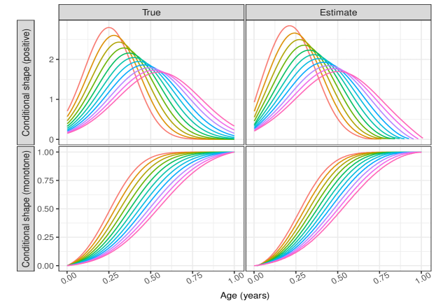
Figure 9: Conditional global Fréchet regression functions for shape trajectories over a dense grid of predictor levels $x$, displayed in red when $x=0.5$ to magenta when $x=1.5$. The left panel displays the “oracle” functions and the right panel illustrates their estimated counterparts, for both positive and monotone functional data.

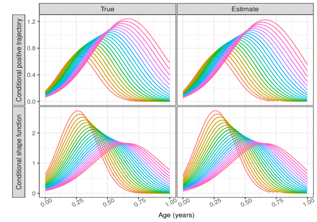
Figure 10: Conditional local Fréchet regression functions in the simulation setting over a dense grid of predictor levels $x$, displayed in red when $x=0.5$ to magenta when $x=1.5$. The left panel displays the “oracle” functions and the right panel illustrates their estimated counterparts, for positive trajectories and their shape components.

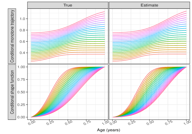
Figure 11: Conditional local Fréchet regression functions in the simulation setting over a dense grid of predictor levels $x$, displayed in red when $x=0.5$ to magenta when $x=1.5$. The left panel displays the “oracle” functions and the right panel illustrates their estimated counterparts, for monotone trajectories and their shape components.

9.2 Decomposition-based Fréchet regression for medfly activity profile data

To explore the effect of survival duration and diet on locomotory activity patterns, we fit a decomposition-based global Fréchet regression model with (estimated) activity trajectories as functional response. We use the decomposition metric $d$ defined in equation (1) of the main paper. The resulting conditional activity trajectories, obtained at five equidistant sample quantiles of age at death, are illustrated in Figure 12. Within each diet group, flies with longer lifespan tend to demonstrate relatively lower daily activity counts. The trajectories overlap at some point between $10$ to $20$ days. This minimal divergence is likely associated with egg-laying activity of the flies, since the flies start laying eggs typically after $10$ days. However, a conventional global Fréchet regression model with functional response fails to elucidate the pattern.

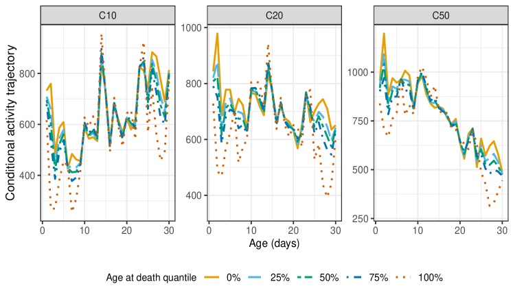
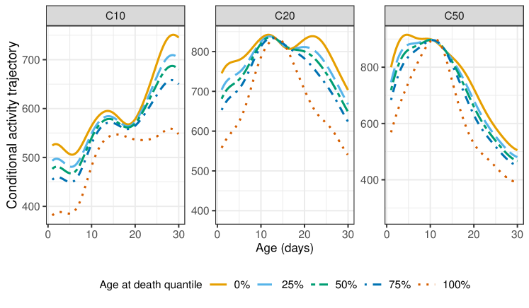
Figure 12: Conditional activity trajectories across varying quantiles of age at death, based on regular (top panel) and decomposition-based (bottom panel) global Fréchet regression model.

9.3 Decomposition-based Fréchet regression for Zürich growth study data

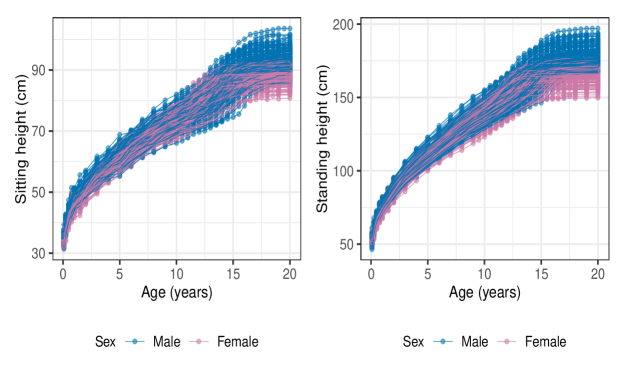
Figure 13: (Left) Sitting height and (right) standing height. Observed height measurements, with connecting lines, for females (pink) and males (blue).

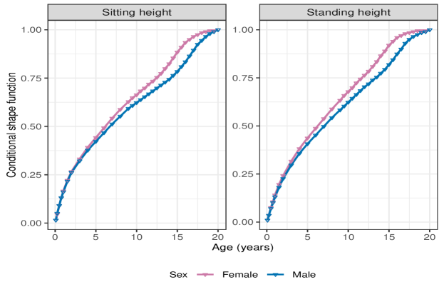
Figure 14: Zürich longitudinal growth study with age-varying sitting (left) and standing height trajectories viewed as monotone functional data. Conditional shape trajectories (CDF) obtained for females (pink) and males (blue), using decomposition-based global Fréchet regression model.

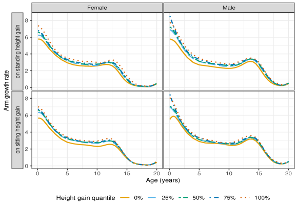
Figure 16: Zürich longitudinal growth study with age-varying arm length trajectories viewed as monotone functional data. Derivatives of fitted arm length trajectories representing corresponding age-varying arm growth rates. Conditional arm growth rate trajectories across varying quantiles of standing (or sitting) height gain for females and males.

REFERENCES

• Bayley and Schaefer (1964) Bayley, N. and E. S. Schaefer (1964). Correlations of maternal and child behaviors with the development of mental abilities: Data from the Berkeley Growth Study. Monographs of the Society for Research in Child Development 29, 1–80.
• Bolstad et al. (2003) Bolstad, B. M., R. A. Irizarry, M. Åstrand, and T. P. Speed (2003). A comparison of normalization methods for high density oligonucleotide array data based on variance and bias. Bioinformatics 19(2), 185–193.
• Carroll et al. (2021) Carroll, C., H.-G. Müller, and A. Kneip (2021). Cross-component registration for multivariate functional data, with application to growth curves. Biometrics 77(3), 839–851.
• Castro et al. (1986) Castro, P. E., W. H. Lawton, and E. Sylvestre (1986). Principal modes of variation for processes with continuous sample curves. Technometrics 28(4), 329–337.
• Chen et al. (2024) Chen, H., H.-G. Müller, V. G. Rodovitis, N. T. Papadopoulos, and J. R. Carey (2024). Daily activity profiles over the lifespan of female medflies as biomarkers of aging and longevity. Aging Cell 23, e14080.
• Chen et al. (2017) Chen, K., P. Delicado, and H.-G. Müller (2017). Modelling function-valued stochastic processes, with applications to fertility dynamics. Journal of the Royal Statistical Society Series B: Statistical Methodology 79(1), 177–196.
• Chen and Lei (2015) Chen, K. and J. Lei (2015). Localized functional principal component analysis. Journal of the American Statistical Association 110(511), 1266–1275.
• Chen and Müller (2012) Chen, K. and H.-G. Müller (2012). Conditional quantile analysis when covariates are functions, with application to growth data. Journal of the Royal Statistical Society Series B: Statistical Methodology 74(1), 67–89.
• Chen et al. (2017) Chen, K., X. Zhang, A. Petersen, and H.-G. Müller (2017). Quantifying infinite-dimensional data: Functional data analysis in action. Statistics in Biosciences 9, 582–604.
• Chen and Samworth (2016) Chen, Y. and R. J. Samworth (2016). Generalized additive and index models with shape constraints. Journal of the Royal Statistical Society Series B: Statistical Methodology 78(4), 729–754.
• Dauxois et al. (1982) Dauxois, J., A. Pousse, and Y. Romain (1982). Asymptotic theory for the principal component analysis of a vector random function: some applications to statistical inference. Journal of Multivariate Analysis 12(1), 136–154.
• Fan (1993) Fan, J. (1993). Local linear regression smoothers and their minimax efficiencies. The Annals of Statistics 21, 196–216.
• Fan and Gijbels (1996) Fan, J. and I. Gijbels (1996). Local Polynomial Modelling and Its Applications: Monographs on Statistics and Applied Probability 66, Volume 66. CRC Press.
• Gajardo and Müller (2021) Gajardo, Á. and H.-G. Müller (2021). Cox Point Process Regression. IEEE Transactions on Information Theory 68(2), 1133–1156.
• Ghosal et al. (2023) Ghosal, R., S. Ghosh, J. Urbanek, J. A. Schrack, and V. Zipunnikov (2023). Shape-constrained estimation in functional regression with Bernstein polynomials. Computational Statistics & Data Analysis 178, 107614.
• Hall et al. (2006) Hall, P., H.-G. Müller, and J.-L. Wang (2006). Properties of principal component methods for functional and longitudinal data analysis. The Annals of Statistics 34(3), 1493 – 1517.
• Hsing and Eubank (2015) Hsing, T. and R. Eubank (2015). Theoretical Foundations of Functional Data Analysis, with an Introduction to Linear Operators, Volume 997. John Wiley & Sons.
• Karhunen (1947) Karhunen, K. (1947). Under lineare methoden in der wahr scheinlichkeitsrechnung. Annales Academiae Scientiarun Fennicae Series A1: Mathematia Physica 47, 1–79.
• Kleffe (1973) Kleffe, J. (1973). Principal components of random variables with values in a seperable hilbert space. Mathematische Operationsforschung und Statistik 4(5), 391–406.
• Loève (1978) Loève, M. (1978). Probability Theory. Vol. II, Graduate Texts in Mathematics. Springer-Verlag.
• Petersen and Müller (2016) Petersen, A. and H.-G. Müller (2016). Functional data analysis for density functions by transformation to a Hilbert space. The Annals of Statistics 44(1), 183–218.
• Petersen and Müller (2019) Petersen, A. and H.-G. Müller (2019). Fréchet regression for random objects with Euclidean predictors. The Annals of Statistics 47(2), 691–719.
• Pya and Wood (2015) Pya, N. and S. N. Wood (2015). Shape constrained additive models. Statistics and Computing 25, 543–559.
• Ramsay et al. (1995) Ramsay, J., R. Bock, and T. Gasser (1995). Comparison of height acceleration curves in the Fels, Zurich, and Berkeley growth data. Annals of Human Biology 22(5), 413–426.
• Ramsay and Silverman (2005) Ramsay, J. and B. Silverman (2005). Functional Data Analysis. Springer.
• Wang et al. (2016) Wang, J.-L., J.-M. Chiou, and H.-G. Müller (2016). Functional Data Analysis. Annual Review of Statistics and Its Application 3, 257–295.
• Zhang and Müller (2011) Zhang, Z. and H.-G. Müller (2011). Functional density synchronization. Computational Statistics & Data Analysis 55(7), 2234–2249.