Neural Approximate Mirror Maps for
Constrained Diffusion Models

Abstract

Diffusion models excel at creating visually-convincing images, but they often struggle to meet subtle constraints inherent in the training data. Such constraints could be physics-based (e.g., satisfying a PDE), geometric (e.g., respecting symmetry), or semantic (e.g., including a particular number of objects). When the training data all satisfy a certain constraint, enforcing this constraint on a diffusion model not only improves its distribution-matching accuracy but also makes it more reliable for generating valid synthetic data and solving constrained inverse problems. However, existing methods for constrained diffusion models are inflexible with different types of constraints. Recent work proposed to learn mirror diffusion models (MDMs) in an unconstrained space defined by a mirror map and to impose the constraint with an inverse mirror map, but analytical mirror maps are challenging to derive for complex constraints. We propose neural approximate mirror maps (NAMMs) for general constraints. Our approach only requires a differentiable distance function from the constraint set. We learn an approximate mirror map that pushes data into an unconstrained space and a corresponding approximate inverse that maps data back to the constraint set. A generative model, such as an MDM, can then be trained in the learned mirror space and its samples restored to the constraint set by the inverse map. We validate our approach on a variety of constraints, showing that compared to an unconstrained diffusion model, a NAMM-based MDM substantially improves constraint satisfaction. We also demonstrate how existing diffusion-based inverse-problem solvers can be easily applied in the learned mirror space to solve constrained inverse problems.

1 Introduction

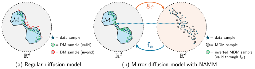
Figure 1: Conceptual illustration. (a) Despite being trained on a data distribution constrained to $\mathcal{M}$, a regular diffusion model (DM) may generate samples that violate the constraint due to learning and/or sampling error. (b) We propose to learn a neural approximate mirror map (NAMM) that entails both a forward map $\mathbf{g}_{\phi}$ and inverse map $\mathbf{f}_{\psi}$. The forward map transforms the constrained space into an unconstrained (“mirror”) space. Once $\mathbf{g}_{\phi}$ and $\mathbf{f}_{\psi}$ are learned, a mirror diffusion model (MDM) can be trained on the pushforward of the data distribution through $\mathbf{g}_{\phi}$. The approximate inverse map $\mathbf{f}_{\psi}$ maps MDM samples back to the constrained space.

Many data distributions follow a rule that is not visually obvious. For example, videos of fluid flow obey a partial differential equation (PDE), but a human may find it difficult to discern whether a given video truly agrees with the prescribed PDE. We can characterize such distributions as constrained distributions. Theoretically, a generative model trained on a constrained image distribution should satisfy the constraint, but in practice, it may generate visually-convincing images that break the rules. Constraint violation is caused by learning error and sampling error [20]. Ensuring constraint satisfaction in spite of learning and sampling errors would make generative models more reliable for applications such as solving inverse problems with physics-informed deep-learned priors.

Diffusion models in particular are popular types of generative models, but existing approaches for incorporating constraints either restrict the type of constraint or do not scale well. Equivariant score-based models [51], Riemannian diffusion models [21, 36], reflected diffusion models [48, 26], log-barrier methods [26], and mirror diffusion models (as originally proposed) [47] are restricted to certain types of constraints, such as symmetry groups [51], Riemannian manifolds [21, 36], or convex sets [26, 47]. Generally speaking, these restrictions are in the service of guaranteeing a hard constraint, whereas a soft constraint offers flexibility and may be sufficient in many scenarios. One could, for example, introduce a guidance term to encourage constraint satisfaction during sampling [32, 6, 71], but so far there does not exist a principled framework to do so. Previous work suggested imposing a soft constraint during training [20] by estimating the clean image at every noisy diffusion step and evaluating its constraint satisfaction. However, approximation [23] of the clean image is extremely crude at high noise levels and thus unsuitable for constraints that are sensitive to approximation error and noise, such as a PDE constraint. Finally, it is always possible to impose the constraint on samples generated by the diffusion model, such as by rejecting invalid samples, either during or after training [37]. However, these approaches rely on computationally-expensive simulation steps. Instead, we aim for a flexible approach to impose general constraints by construction.

Our goal is to find an invertible function that maps constrained images into an unconstrained space so that a regular generative model can be trained in the unconstrained space and automatically satisfy the constraint through the inverse function. We propose neural approximate mirror maps (NAMMs), which bring the flexibility of soft constraints into the principled framework of mirror diffusion models [47]. A mirror diffusion model (MDM) allows for training a completely unconstrained diffusion model in a “mirror” space defined by a mirror map. Unconstrained samples from the trained diffusion model are mapped back to the constrained space via an inverse mirror map. However, invertible mirror maps are challenging to derive in closed form for general (e.g., non-convex) constraints.

A NAMM encompasses a (forward) mirror map $\mathbf{g}_{\phi}$ and its approximate inverse map $\mathbf{f}_{\psi}$, which are trained to offer the desired benefits of an analytical mirror map. In particular, $\mathbf{f}_{\psi}\approx\mathbf{g}_{\phi}^{-1}$, and $\mathbf{f}_{\psi}$ maps unconstrained points to the constrained space (see Fig. 1 for a conceptual illustration). Our method works for any constraint that has a differentiable function to quantify the distance from an image to the constraint set. We parameterize $\mathbf{g}_{\phi}$ as the gradient of a strongly input-convex neural network (ICNN) [4] to satisfy invertibility. We train the NAMM with a cycle-consistency loss [73] to ensure $\mathbf{f}_{\psi}\approx{\mathbf{g}_{\phi}}^{-1}$ and train the inverse map with a constraint loss to ensure $\mathbf{f}_{\psi}(\tilde{\mathbf{x}})$ is close to the constraint set for all $\tilde{\mathbf{x}}$ that we are interested in (we will define this more formally). An MDM can be trained on the pushforward of the data distribution through $\mathbf{g}_{\phi}$, and its generated samples can be mapped to the constraint set via $\mathbf{f}_{\psi}$. Although not inherently restricted to diffusion models, our approach maintains the many advantages of diffusion models, including expressive generation, simulation-free training [62], and tractable computation of probability densities [47]. One can also adapt existing diffusion-based inverse solvers for the mirror space and enforce constraints with the inverse map.

Through our experiments, we show improved constraint satisfaction for various physics-based, geometric, and semantic constraints. We demonstrate how a NAMM can be used to solve constrained inverse problems, such as data assimilation. Finally, we validate the soundness of the method through several ablation studies, in particular finding that modeling the mirror map as the gradient of a strongly-convex function brings not just theoretical, but also practical, benefits.

2 Background

2.1 Constrained generative models

Explicitly incorporating a data constraint into a generative model poses benefits such as data efficiency [28, 8], generalization capabilities [45], and feasibility of samples [31]. Some methods leverage equivariant neural networks [57, 30, 66] for symmetry [3, 51, 43, 64, 11, 55, 29, 45, 50, 22, 69, 34, 70] but do not generalize to other types of constraints and are often restricted to a certain type of generative model (e.g., flow-based or score-based models) [43, 64, 11, 55, 29, 45, 50, 51, 69, 34, 70, 22, 3]. Recent work has studied constrained diffusion models, including Riemannian diffusion models [21, 36], log-barrier methods [26], reflected diffusion models [48], and mirror diffusion models [47]. However, these methods make strong assumptions about the constraint, such as being characterized as a Riemannian manifold [21, 36], having a well-defined reflection operator [48], or corresponding to a convex constraint set [26, 47]. Fishman et al. [27] proposed a diffusion model that incorporates Metropolis-Hastings steps to be compatible with a general constraint, but impractically high rejection rates may occur with constraints that are challenging to satisfy, such as a PDE constraint.

An alternative approach is to introduce a soft constraint penalty when training the generative model [28, 49, 15, 31, 20]. However, evaluating the constraint loss of generated samples during training may be prohibitively expensive. Instead, one could add constraint-violating training examples [31], but it is often difficult to procure useful negative examples. In contrast to previous soft approaches, our approach does not alter the training objective of the generative model.

2.2 Mirror maps

For any convex constraint set $\mathcal{C}\subseteq\mathbb{R}^{d}$, one can define a mirror map that maps from the constraint set to all of $\mathbb{R}^{d}$. This is done by first defining a mirror potential $\phi:\mathcal{C}\to\mathbb{R}$ that is continuously-differentiable and strongly-convex [12, 65]. The mirror map is defined as the gradient $\nabla\phi:\mathcal{C}\to\mathbb{R}^{d}$ [47]. Importantly, every mirror map has an inverse $(\nabla\phi)^{-1}:\mathbb{R}^{d}\to\mathcal{C}$. Unlike the forward mirror map, the inverse map is not necessarily the gradient of a strongly-convex function [72, 65]. Mirror maps have been used for constrained optimization [9] and constrained sampling [35, 46, 47].

Although true mirror maps exist only for convex constraint sets, we seek to generalize the concept to learn approximate mirror maps that handle more complex constraint sets. Recent work suggested learning mirror maps for purposes such as convex optimization [65] and reinforcement learning [2] but did not tackle constrained generative modeling.

2.3 Diffusion models

A diffusion model is a type of generative model that learns to generate new data samples through a gradual denoising process [58, 33, 60, 62, 42]. The diffusion, or noising, process can be modeled as a stochastic differential equation (SDE) [62]. The diffusion SDE induces a time-dependent image distribution $p_{t}$, where $p_{0}=p_{\text{data}}$ (the target image distribution) and $p_{T}\approx\mathcal{N}(\mathbf{0},\mathbf{I})$. The goal of a diffusion model is to generate new images by reversing the diffusion process. This can be done with the score function of $p_{t}$, defined as $\nabla_{\mathbf{x}}\log p_{t}(\mathbf{x})$. In the context of imaging problems, the score function is often parameterized using a convolutional neural network (CNN) with parameters $\theta$, which we denote by $\mathbf{s}_{\theta}$. The score model is trained with a “denoising score matching” objective [38, 67, 62] that allows the time-dependent score to be learned in a simulation-free manner (i.e., it does not require simulating the forward noising process during training). The score function appears in a reverse-time SDE [62, 5] that can be used to sample from the clean image distribution $p_{0}$ by first sampling an image of pure noise from $\mathcal{N}(\mathbf{0},\mathbf{I})$ and then gradually denoising it.

3 Method

We will now describe neural approximate mirror maps (NAMMs) for constrained diffusion models. While we focus on diffusion models, any generative model can be trained in the learned mirror space. We denote the constrained image distribution by $p_{\text{data}}$ and the (not necessarily convex) constraint set by $\mathcal{M}\subseteq\mathbb{R}^{d}$. Images in the constrained space and mirror space are denoted by $\mathbf{x}$ and $\tilde{\mathbf{x}}$, respectively.

3.1 Learning the forward and inverse mirror maps

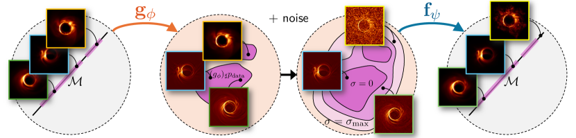
Figure 2: NAMM training illustration. Given data that lie on a constraint manifold $\mathcal{M}$ (e.g., the hyperplane of images with the same total brightness), we jointly train an approximate mirror map $\mathbf{g}_{\phi}$ and its approximate inverse $\mathbf{f}_{\psi}$. After mapping data $\mathbf{x}\sim p_{\text{data}}$ to the mirror space as $\mathbf{g}_{\phi}(\mathbf{x})$, we perturb them with additive Gaussian noise whose std. dev. can be anywhere between $0$ and $\sigma_{\text{max}}$. The inverse map $\mathbf{f}_{\psi}$ is trained to map these perturbed samples back onto $\mathcal{M}$.

Let $\mathbf{g}_{\phi}$ and $\mathbf{f}_{\psi}$ be the neural networks modeling the forward and inverse mirror maps, respectively, where $\phi$ and $\psi$ are their parameters. We formulate the following learning problem:

$$\phi^{*},\psi^{*}\in\operatorname*{arg\,min}_{\phi,\psi}\bigg{\{}\mathcal{L}_{\text{cycle}}(\mathbf{g}_{\phi},\mathbf{f}_{\psi})+\lambda_{\text{constr}}\mathcal{L}_{\text{constr}}(\mathbf{g}_{\phi},\mathbf{f}_{\psi})+\lambda_{\text{reg}}\mathcal{R}(\mathbf{g}_{\phi})\bigg{\}},$$ (1)

where $\mathcal{L}_{\text{cycle}}$ encourages $\mathbf{g}_{\phi}$ and $\mathbf{f}_{\psi}$ to be inverses of each other; $\mathcal{L}_{\text{constr}}$ encourages $\mathbf{f}_{\psi}$ to map unconstrained points back to the constraint set; and $\mathcal{R}$ is a regularization term to ensure there is a unique solution for the maps. Here $\lambda_{\text{constr}},\lambda_{\text{reg}}\in\mathbb{R}_{>0}$ are scalar hyperparameters.

A true inverse mirror map satisfies cycle consistency and constraint satisfaction on all of $\mathbb{R}^{d}$, so ideally $\mathbf{f}_{\psi}(\tilde{\mathbf{x}})=\mathbf{g}_{\phi}^{-1}(\tilde{\mathbf{x}})$ and $\mathbf{f}_{\psi}(\tilde{\mathbf{x}})\in\mathcal{M}$ for all $\tilde{\mathbf{x}}\in\mathbb{R}^{d}$. But since it would be computationally infeasible to optimize $\mathbf{f}_{\psi}$ over all possible points in $\mathbb{R}^{d}$, we instead optimize it over distributions that we would expect the inverse map to face in practice in the context of diffusion models. That is, we only need $\mathbf{f}_{\psi}$ to be valid for samples from an MDM trained on ${(\mathbf{g}_{\phi})}_{\sharp}p_{\text{data}}$, which we refer to as the mirror distribution. To make $\mathbf{f}_{\psi}$ robust to learning/sampling error of the MDM, we consider a sequence of noisy distributions in the mirror space, each corresponding to adding Gaussian noise to samples from ${(\mathbf{g}_{\phi})}_{\sharp}p_{\text{data}}$, which, given a maximum perturbation level $\sigma_{\text{max}}$, we denote by

$$\left({(\mathbf{g}_{\phi})}_{\sharp}p_{\text{data}}\ast\mathcal{N}(\mathbf{0},\sigma^{2}\mathbf{I})\right)_{\sigma\in[0,\sigma_{\text{max}}]}.$$ (2)

We train $\mathbf{f}_{\psi}$ to be a valid inverse mirror map only for points from these noisy mirror distributions. Since we do not know a priori how much noise the MDM samples will contain, we consider all possible noise levels up to $\sigma_{\text{max}}$ for robustness (see Appendix A.2 for an ablation study of this choice).

We define the following cycle-consistency loss [73], which covers both the forward and inverse directions and evaluates the inverse direction for the entire sequence of distributions defined in Eq. 2:

$$\mathcal{L}_{\text{cycle}}(\mathbf{g}_{\phi},\mathbf{f}_{\psi}):=\mathbb{E}_{\mathbf{x}\sim p_{\text{data}}}\bigg{[}\left\lVert\mathbf{x}-\mathbf{f}_{\psi}\left(\mathbf{g}_{\phi}(\mathbf{x})\right)\right\rVert_{1}\\ +\int_{0}^{\sigma_{\text{max}}}\mathbb{E}_{\mathbf{z}\sim\mathcal{N}(\mathbf{0},\mathbf{I})}\left[\left\lVert\mathbf{g}_{\phi}(\mathbf{x})+\sigma\mathbf{z}-\mathbf{g}_{\phi}\left(\mathbf{f}_{\psi}(\mathbf{g}_{\phi}(\mathbf{x})+\sigma\mathbf{z})\right)\right\rVert_{1}\right]\bigg{]}.$$ (3)

Let $\ell_{\text{constr}}:\mathbb{R}^{d}\to\mathbb{R}_{\geq 0}$ be a differentiable constraint distance that measures the distance from an input image to the constraint set. We define the following constraint loss to encourage $\mathbf{f}_{\psi}$ to map points from the noisy mirror distributions (Eq. 2) to the constraint set:

$$\mathcal{L}_{\text{constr}}(\mathbf{g}_{\phi},\mathbf{f}_{\psi}):=\mathbb{E}_{\mathbf{x}\sim p_{\text{data}}}\left[\int_{0}^{\sigma_{\text{max}}}\mathbb{E}_{\mathbf{z}\sim\mathcal{N}(\mathbf{0},\mathbf{I})}\left[\ell_{\text{constr}}\left(\mathbf{f}_{\psi}(\mathbf{g}_{\phi}(\mathbf{x})+\sigma\mathbf{z})\right)\right]\mathrm{d}\sigma\right].$$ (4)

To ensure a unique solution, we regularize $\mathbf{g}_{\phi}$ to be close to the identity function:

$$\mathcal{R}(\mathbf{g}_{\phi}):=\mathbb{E}_{\mathbf{x}\sim p_{\text{data}}}\left[\left\lVert\mathbf{x}-\mathbf{g}_{\phi}(\mathbf{x})\right\rVert_{1}\right].$$ (5)

We use Monte-Carlo to approximate the expectations in the objective over the noisy mirror distributions with $\sigma\sim\mathcal{U}([0,\sigma_{\text{max}}])$ and approximately solve Eq. 1 with stochastic gradient descent.

Architecture

We parameterize $\mathbf{g}_{\phi}$ as the gradient of an input-convex neural network (ICNN) following the implementation of Tan et al. [65], thus satisfying the requirement of being the gradient of a strongly-convex function. We note that $\mathbf{g}_{\phi}$ is not a true mirror map since $\mathcal{M}$ is not assumed to be convex, and $\mathbf{g}_{\phi}$ is defined on all of $\mathbb{R}^{d}$ instead of just on $\mathcal{M}$. We parameterize $\mathbf{f}_{\psi}$ as a ResNet-based CNN similar to the one used in CycleGAN [73]. Note that $\mathbf{f}_{\psi}$ is also the gradient of a strongly-convex function if the cycle-consistency loss is $0$ (i.e., $\mathbf{f}_{\psi}=\mathbf{g}_{\phi}^{-1}$).

3.2 Learning the mirror diffusion model

Similarly to Liu et al. [47], we train an MDM on the mirror distribution ${(\mathbf{g}_{\phi})}_{\sharp}p_{\text{data}}$ and map its samples to the constrained space through $\mathbf{f}_{\psi}$. In particular, we train a score model $\mathbf{s}_{\theta}$ with the following denoising score matching objective in the learned mirror space (defined as the range of $\mathbf{g}_{\phi}$):

$$\theta^{*}\in\operatorname*{arg\,min}_{\theta}\mathbb{E}_{t}\left\{\lambda(t)\mathbb{E}_{\tilde{\mathbf{x}}(0)\sim{(\mathbf{g}_{\phi})}_{\sharp}p_{\text{data}}}\mathbb{E}_{\tilde{\mathbf{x}}(t)\mid\tilde{\mathbf{x}}(0)}\left[\left\lVert\tilde{\mathbf{s}}_{\theta}\left(\tilde{\mathbf{x}}(t),t\right)-\nabla_{\tilde{\mathbf{x}}(t)}\log p_{0t}\left(\tilde{\mathbf{x}}(t)\mid\tilde{\mathbf{x}}(0)\right)\right\rVert_{2}^{2}\right]\right\},$$ (6)

where $\tilde{\mathbf{x}}(0)\sim{(\mathbf{g}_{\phi})}_{\sharp}p_{\text{data}}$ is obtained as $\tilde{\mathbf{x}}(0):=\mathbf{g}_{\phi}(\mathbf{x}(0))$ for $\mathbf{x}(0)\sim p_{\text{data}}$. Here $p_{0t}$ denotes the transition kernel from $\tilde{\mathbf{x}}(0)$ to $\tilde{\mathbf{x}}(t)$ under the diffusion SDE, and $\lambda(t)\in\mathbb{R}_{>0}$ is a time-dependent weight. To sample new images, we sample $\tilde{\mathbf{x}}(T)\sim\mathcal{N}(\mathbf{0},\mathbf{I})$, run reverse diffusion in the mirror space, and map the resulting $\tilde{\mathbf{x}}(0)$ to the constrained space via $\mathbf{f}_{\psi}$.

3.3 Finetuning the inverse mirror map

The inverse map $\mathbf{f}_{\psi}$ is trained with samples from the noisy mirror distributions in Eq. 2, but we ultimately wish to evaluate $\mathbf{f}_{\psi}$ with samples from the MDM. To reduce the distribution shift, it may be helpful to finetune $\mathbf{f}_{\psi}$ with MDM samples. In the following finetuning objective, we replace $\tilde{\mathbf{x}}\sim{(\mathbf{g}_{\phi})}_{\sharp}p_{\text{data}}$ with $\tilde{\mathbf{x}}\sim p_{\theta}$, where $p_{\theta}$ is the distribution of MDM samples in the mirror space:

$$\psi^{*}=\operatorname*{arg\,min}_{\psi}\Bigg{\{}\mathbb{E}_{\mathbf{x}\sim p_{\text{data}}}\left\lVert\mathbf{x}-\mathbf{f}_{\psi}(\mathbf{g}_{\phi}(\mathbf{x}))\right\rVert_{1}\\ +\mathbb{E}_{\tilde{\mathbf{x}}\sim p_{\theta}}\Bigg{[}\int_{0}^{\sigma_{\text{max}}}\mathbb{E}_{\mathbf{z}\sim\mathcal{N}(\mathbf{0},\mathbf{I})}\big{[}\left\lVert\tilde{\mathbf{x}}+\sigma\mathbf{z}-\mathbf{g}_{\phi}(\mathbf{f}_{\psi}(\tilde{\mathbf{x}}+\sigma\mathbf{z}))\right\rVert_{1}+\lambda_{\text{constr}}\ell_{\text{constr}}\left(\mathbf{f}_{\psi}(\tilde{\mathbf{x}}+\sigma\mathbf{z})\right)\big{]}\mathrm{d}\sigma\Bigg{]}\Bigg{\}}.$$ (7)

Finetuning essentially tailors $\mathbf{f}_{\psi}$ to the MDM. The original objective assumes that the MDM will sample Gaussian-perturbed images from the mirror distribution, but in reality it samples from a slightly different distribution. We generate a training dataset of samples $\tilde{\mathbf{x}}$ from the MDM and then finetune the inverse map to deal with such samples specifically.

4 Results

We present experiments with constraints ranging from physics-based to semantic, finding improved constraint satisfaction with greater training efficiency. Appendices A.1 and B provide implementation and constraint details, respectively. The following paragraphs introduce the demonstrated constraints $\ell$. For each constraint, we consider an image dataset for which the constraint is physically meaningful.

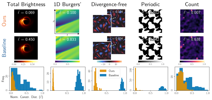
Figure 3: Improved constraint satisfaction. Samples from our approach are nearly indistinguishable from baseline samples, yet there is a significant difference in their distances from the constraint set. The baseline is a DM trained on the original constrained dataset. Our approach is to train a NAMM and then an MDM in the mirror space induced by $\mathbf{g}_{\phi}$. Samples are obtained by sampling from the MDM and then passing samples through $\mathbf{f}_{\psi}$. The histograms show normalized constraint distances $\bar{\ell}$ of $128$ samples (normalized so that each constraint has a maximum of $1$ across the samples from both methods). Our results are from the finetuned NAMM. For each constraint, we made sure that the DM was trained for at least as long as the NAMM, MDM, and finetuned NAMM combined.

Total brightness

In astronomical imaging, even if the structure of a source is unknown a priori, often the total brightness, or total flux, is well constrained [24, 25]. We define $\ell_{\text{flux}}(\mathbf{x})$ as the absolute difference between the sum of the pixel values in $\mathbf{x}$ and the true total brightness. For demonstration, we use a dataset of $64\times 64$ images of black-hole simulations [68] whose pixel values sum to $120$.

1D Burgers’

We consider Burgers’ equation [7, 13] for a 1D viscous fluid, representing the discretized solution as an $n_{x}\times n_{t}$ image $\mathbf{x}$, where $n_{x}$ and $n_{t}$ are the numbers of grid points in space and time, respectively. The distance $\ell_{\text{burgers}}(\mathbf{x})$ compares each 1D state in the image to the PDE solver’s output given the previous state (based on Crank-Nicolson time-discretization [19, 41]). The dataset consists of $64\times 64$ images with Gaussian random fields as initial conditions.

Divergence-free

A time-dependent 2D velocity field $\mathbf{u}=\mathbf{u}(x,y,t)$ is called divergence-free or incompressible if $\nabla\cdot\mathbf{u}=0$. We define the constraint distance $\ell_{\text{div}}$ as the $\ell^{1}$-norm of the divergence and demonstrate this constraint with 2D Kolmogorov flows [14, 10, 56]. We represent the trajectory of the 2D velocity, discretized in space-time, as a two-channel (for both velocity components) image $\mathbf{x}$ with the states appended sequentially. We used jax-cfd [44] to generate trajectories of eight $64\times 64$ states and appended them in a $2\times 4$ pattern to create $128\times 256$ images.

Periodic

To demonstrate a symmetry constraint, we consider images $\mathbf{x}$ that are periodic tilings of a unit cell. This type of symmetry appears in materials science, such as when constructing metamaterials out of unit cells [52]. We use a distance function $\ell_{\text{periodic}}$ that compares all pairs of tiles in the image and computes the average $\ell^{1}$-norm of their differences. We created a dataset of $64\times 64$ images (composed of $32\times 32$ unit cells tiled in a $2\times 2$ fashion) using the code of Ogren et al. [52].

Count

Generative models are known to sometimes generate the incorrect number of objects [53]. We formulate a differentiable count constraint by relying on a CNN to estimate the count of a particular object in an image $\mathbf{x}$. Note that using a neural network leads to a non-analytical and highly non-convex constraint. Letting $f_{\text{CNN}}:\mathbb{R}^{d}\to\mathbb{R}$ be the trained counting CNN, we use the distance function $\ell_{\text{count}}(\mathbf{x}):=\left\lvert f_{\text{CNN}}(\mathbf{x})-\bar{c}\right\rvert$ for a target count $\bar{c}$. The constraint dataset consists of $128\times 128$ simulated images of exactly eight (8) radio galaxies with background noise [18].

4.1 Improved constraint satisfaction and training efficiency

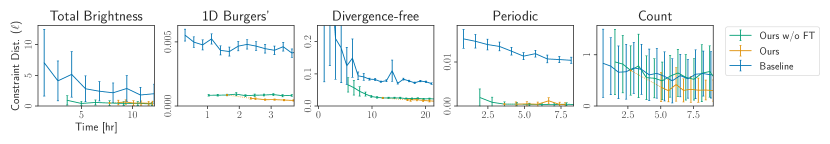
Figure 4: Training efficiency. For each method, we clocked the total compute time during training (ignoring validation and I/O operations) and here plot the mean $\pm$ std. dev. of the constraint distances $\ell$ of $128$ generated samples at each checkpoint. The MDM training curve (“Ours w/o FT”) is offset by the time it took to train the NAMM. The finetuning curve (“Ours”) is offset by the time it took to train the NAMM and MDM and generate finetuning data. For most constraints, the DM has consistently higher constraint distance without any sign of converging to the same performance as that of the MDM. For the count constraint, the MDM performs on par with the DM, but finetuning noticeably accelerates constraint satisfaction. Each run was done on the same hardware ($4\times$ A100 GPUs).

First and foremost, we verify that our approach leads to better constraint satisfaction than a vanilla diffusion model (DM). We evaluate constraint satisfaction by computing the average constraint distance of generated samples. We note that since the constraint distance is non-negative, an average constraint distance of $0$ implies that the constraint is satisfied almost surely.

For each constraint, we trained a NAMM on the corresponding dataset and then trained an MDM on the pushforward of the dataset through the learned $\mathbf{g}_{\phi}$. We show results from a finetuned NAMM, but as we discuss in Sec. 4.3, finetuning is often not necessary. For a baseline, we trained a DM on the original dataset. Fig. 3 highlights that our MDM samples inverted through $\mathbf{f}_{\psi}$ are closer to the constraint set than DM samples. Our samples and the DM samples are visually indistinguishable, yet their constraint distances can be drastically different. For the total brightness, 1D Burgers’, divergence-free, and periodic constraints, there is a significant gap between our distribution of constraint distances and the baseline distribution. The gap is smaller, although still notable, for the count constraint, which may be due to difficulty of optimizing a highly non-convex constraint.

Furthermore, our approach achieves better constraint satisfaction in less training time. In Fig. 4, we plot constraint satisfaction as a function of compute time, comparing our approach (with and without finetuning) to the DM. Accounting for the time it takes to train the NAMM, our NAMM-based MDM achieves much lower constraint distances than the DM for the three physics-based constraints and the periodic constraint, often reaching a level that the DM struggles to achieve. For the count constraint, we find that finetuning is essential for improving constraint satisfaction, and it is more time-efficient to finetune the inverse map than to continue training the MDM.

4.2 Solving constrained inverse problems with mirror DPS

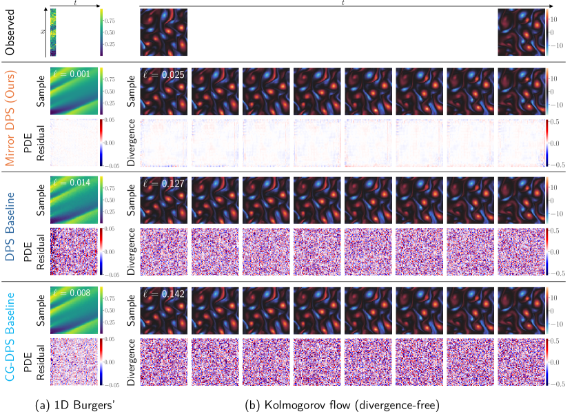
Figure 5: Data assimilation. We used the same finetuned NAMM, MDM, and DM checkpoints as in Fig. 3. (a) Given noisy observations of the first eight states, we sampled possible full trajectories of a 1D Burgers’ system. Our solutions have smaller deviation from the PDE than samples obtained with DPS, even those of constraint-guided DPS (CG-DPS). (b) The task is to infer the full Kolmogorov flow from noisy observations of the first and last states. Our solution has significantly less divergence.

Many methods have been proposed to use a pretrained diffusion model to sample images from the posterior distribution $p(\mathbf{x}\mid\mathbf{y})\propto p(\mathbf{y}\mid\mathbf{x})p(\mathbf{x})$ [16, 32, 63, 39, 40, 59], given measurements $\mathbf{y}\in\mathbb{R}^{m}$ and a diffusion-model prior $p(\mathbf{x})$. One of the most popular methods is diffusion posterior sampling (DPS) [17]. To adapt DPS for the mirror space, we simply evaluate the measurement likelihood on inverted mirror images $\mathbf{f}_{\psi}(\tilde{\mathbf{x}})$ instead of on images $\mathbf{x}$ in the original space.

We demonstrate mirror DPS on data assimilation, an inverse problem that aims to recover the hidden state of a dynamical system given imperfect observations of the state. In Fig. 5, we show results for data assimilation of a 1D Burgers’ system and a divergence-free Kolmogorov flow given a few noisy state observations, which can be essentially formulated as a denoise-and-inpaint problem. For each case, we used mirror DPS with the corresponding NAMM-based MDM. We include two baselines: (1) vanilla DPS with the DM and (2) constraint-guided DPS (CG-DPS) with the DM. The latter incorporates the constraint distance as an additional likelihood term. As Fig. 5 shows, our approach leads to notably less constraint violation (i.e., less deviation from the PDE or less divergence) than both baselines. Appendix A.3 shows that our method consistently outperforms the baselines for different measurement-likelihood and constraint-guidance weights used in DPS and CG-DPS.

4.3 Ablation studies

Finetuning

Tab. 1 shows the improvement in constraint satisfaction after finetuning $\mathbf{f}_{\psi}$. We also verify that the resulting image distribution does not become drastically different from the true distribution by using average cosine distance between PCA components as a proxy for the similarity of the true and generated distributions. We find that finetuning does not significantly change the distribution-matching accuracy and in some cases improves it while improving constraint satisfaction.

		Total Brightness	1D Burgers’	Divergence-free	Periodic	Count
Before FT	Constr. dist. ($\downarrow$)	$0.49\pm 0.38$	$0.09\pm 0.01$	$2.52\pm 0.20$	$0.05\pm 0.06$	$0.73\pm 0.53$
	PCA dist. ($\downarrow$)	$\mathbf{0.99}$	$\mathbf{0.98}$	$0.98$	$\mathbf{1.03}$	$1.00$
After FT	Constr. dist. ($\downarrow$)	$\mathbf{0.49\pm 0.30}$	$\mathbf{0.04\pm 0.00}$	$\mathbf{1.42\pm 0.32}$	$\mathbf{0.04\pm 0.06}$	$\mathbf{0.36\pm 0.26}$
	PCA dist. ($\downarrow$)	$1.01$	$1.00$	$\mathbf{0.97}$	$\mathbf{1.03}$	$\mathbf{0.96}$

Table 1: Effect of finetuning. Constr. dist. (mean $\pm$ std. dev. of $128$ inverted MDM samples) is computed as $10\lambda_{\text{constr}}\ell$. PCA dist. is the average cosine distance between the learned distribution’s principal components and the true distribution’s principal components. PCA was done with $50$ components and approximated with $128$ inverted MDM samples and all the samples from the true test data. PCA dist. is a rough proxy that we use to confirm that finetuning does not significantly change the MDM’s distribution-matching accuracy while improving the constraint distance. For relatively simple constraints (e.g., total brightness and periodic), finetuning is not critical.

Constraint loss hyperparameters

There are two hyperparameters for the constraint loss in Eq. 1: $\sigma_{\text{max}}$ determines how much noise to add to samples from the mirror distribution, and $\lambda_{\text{constr}}$ is the weight of the constraint loss. Intuitively, a higher $\sigma_{\text{max}}$ means that the inverse map $\mathbf{f}_{\psi}$ must map larger regions of $\mathbb{R}^{d}$ back to the constraint set, making its learning objective more challenging. We would expect the forward map $\mathbf{g}_{\phi}$ to cooperate by maintaining a reasonable SNR in the noisy mirror distributions. For example, Fig. 6 shows how increasing $\sigma_{\text{max}}$ causes $\mathbf{g}_{\phi}(\mathbf{x})$ for $\mathbf{x}\sim p_{\text{data}}$ to have larger magnitudes so that the added noise will not hide the signal. However, setting $\sigma_{\text{max}}$ too high can worsen constraint satisfaction, perhaps due to the challenge of finding an inverse map that effectively maps the larger sequence of noisy distributions back to the constraint set. On the flip side, setting $\sigma_{\text{max}}$ too low can also worsen constraint satisfaction because of poor robustness of $\mathbf{f}_{\psi}$. Meanwhile, increasing $\lambda_{\text{constr}}$ for the same $\sigma_{\text{max}}$ leads to lower constraint distance, although there is a tradeoff between constraint distance and cycle-consistency inherent in the NAMM objective (Eq. 1).

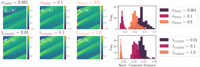
Figure 6: Effect of $\sigma_{\text{max}}$ and $\lambda_{\text{constr}}$, demonstrated with 1D Burgers’. First row: as $\sigma_{\text{max}}$ increases (keeping $\lambda_{\text{constr}}=1.0$), the mirror image $\mathbf{g}_{\phi}(\mathbf{x})$ for $\mathbf{x}\sim p_{\text{data}}$ increases in magnitude to maintain a similar SNR. Histograms show constraint distances of $128$ inverted MDM samples, normalized to have a maximum of 1 across the samples from all three settings. Decreasing $\sigma_{\text{max}}$ from $0.5$ to $0.1$ improves the constraint distances, but further lowering it to $0.001$ causes the constraint distances to go back up. This indicates a tradeoff between robustness and performance of $\mathbf{f}_{\psi}$. Second row: as $\lambda_{\text{constr}}$ increases (keeping $\sigma_{\text{max}}=0.1$), $\mathbf{g}_{\phi}(\mathbf{x})$ does not change as much as when increasing $\sigma_{\text{max}}$, but the constraint distances decrease (with a tradeoff in cycle consistency). For all three settings, the same number of NAMM and MDM epochs was used as in Fig. 3 but without finetuning.

Mirror map parameterization

Fig. 7 compares parameterizing $\mathbf{g}_{\phi}$ as the gradient of an ICNN versus as a ResNet-based CNN. We find that the ICNN approach has practical benefits in addition to being theoretically justified. For the 1D Burgers’ and divergence-free constraints, we demonstrate how the mirror space changes when instead parameterizing the forward map as a ResNet-based CNN. The mirror space becomes less regularized, leading to worse constraint satisfaction of the MDM. A possible explanation is that the MDM struggles to learn a less-regularized mirror space.

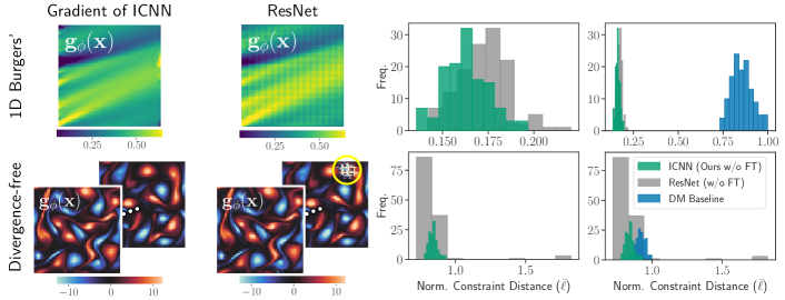
Figure 7: Parameterizing $\mathbf{g}_{\phi}$ as gradient of ICNN vs. as ResNet-based CNN. Both types of mirror maps preserve some visual similarity, but using an ICNN better regularizes the mirror space. The ResNet mirror images include irregularities, such as the patch circled in yellow in the divergence-free example. The histograms show the normalized constraint distances $\bar{\ell}$ of $128$ inverted MDM samples (without finetuning). The rightmost histograms include the DM results from Fig. 3 for comparison. As the histograms show, an ICNN leads to better constraint satisfaction with fewer outliers. We followed the number of NAMM and MDM epochs used in Fig. 3 for both constraints without finetuning. We found that even with finetuning, a ResNet-based forward map still leads to inverted MDM samples of worse constraint satisfaction or noticeably worse visual quality.

5 Conclusion

Limitations

Our approach does not guarantee exact constraint satisfaction. The advantage is greater flexibility with the constraint, as we only require a differentiable constraint distance. As we saw with the count constraint, the constraint loss may not always be easy to optimize via gradient-based methods. Finally, there are many fruitful theoretical questions to pursue, such as formulating guarantees on the quality of the learned mirror map in relation to different classes of constraints.

Summary

We have proposed a method for constrained diffusion models that minimally restricts the generative model and constraint. A NAMM consists of a mirror map $\mathbf{g}_{\phi}$ and its approximate inverse $\mathbf{f}_{\psi}$, which is robust to noise added to samples in the mirror space induced by $\mathbf{g}_{\phi}$. One can train a mirror diffusion model in this mirror space to generate samples that are constrained by construction via the inverse map. We have validated that our method provides significantly better constraint satisfaction than a vanilla diffusion model on various constraints and have shown its utility for solving constrained inverse problems. Our work establishes that neural approximate mirror maps effectively rein in generative models according to visually-subtle yet physically-meaningful constraints.

Appendix A Experiment details

A.1 Implementation

MDM score model

For training the score model $s_{\theta}$ in the learned mirror space, we followed the implementation of Song et al. [61]. We used the NCSN++ architecture with $64$ filters in the first layer and the VP SDE with $\beta_{\min}=0.1$ and $\beta_{\max}=20$. Training was done using the Adam optimizer with a learning rate of $0.0002$ and gradient norm clipping with a threshold of $1$.

NAMM

For $\mathbf{g}_{\phi}$, we followed the implementation of the gradient of a strongly-convex ICNN of Tan et al. [65], configuring the ICNN to be $0.9$-strongly convex. Following the settings of CycleGAN [73], $\mathbf{f}_{\psi}$ was implemented as a ResNet-based generator with $6$ residual blocks and $32$ filters in the last convolutional layer. For all constraints except the divergence-free constraint, we had the ResNet-based generator output the residual image (i.e., $\mathbf{f}_{\psi}(\tilde{\mathbf{x}})=\text{ResNet}(\tilde{\mathbf{x}})+\tilde{\mathbf{x}}$). We found that for the divergence-free constraint, a non-residual-based inverse map (i.e., $\mathbf{f}_{\psi}(\tilde{\mathbf{x}})=\text{ResNet}(\tilde{\mathbf{x}})$) achieves better constraint loss. The NAMM was trained using Adam optimizer with a learning rate of $0.001$ for the divergence-free constraint and a learning rate of $0.0002$ for all other demonstrated constraints.

Tab. 2 shows the hyperparameter choices for each constraint. The regularization weight $\lambda_{\text{reg}}$ in the NAMM objective (Eq. 1) was fixed at $0.001$. We used $3$ ICNN layers for images $64\times 64$ or smaller and $2$ ICNN layers for images $128\times 128$ or larger for the sake of efficiency. These hyperparameter values do not need to be heavily tuned, as we chose these settings through a coarse parameter search (e.g., trying $\lambda_{\text{constr}}=0.01$ or $\lambda=1$ to see which would lead to reasonable loss curves).

	Num. ICNN layers	$\sigma_{\text{max}}$	$\lambda_{\text{constr}}$
Total Flux	$3$	$0.1$	$0.01$
1D Burgers’	$3$	$0.1$	$1$
Divergence-free	$2$	$0.5$	$1$
Periodic	$3$	$0.1$	$1$
Count	$2$	$0.1$	$0.01$

Table 2: NAMM hyperparameter values for each constraint in our experiments.

The main results shown in Fig. 3 were taken from the finetuned NAMM, ensuring that the total training time of the NAMM, MDM, and finetuning did not exceed the total training time of the baseline DM. While we kept track of the validation loss, this was not used to determine stopping time. We found that the NAMM training and MDM training were not prone to overfitting, so we chose the total number of epochs based on observing a reasonable level of convergence of the loss curves. We found that some overfitting is possible during finetuning but did not perform early stopping. All results were obtained from unseen test data because we fed random samples from the MDM into the inverse map and made sure not to use the same random seed as the one used to generate finetuning data. For all constraints, we generated $12800$ training examples from the MDM for finetuning.

Tab. 3 details the exact number of training epochs for each constraint. Fig. 4 in the main results compares the constraint distances of our method without finetuning, our method with finetuning, and the baseline DM as a function of compute time.

	NAMM epochs
	(before FT)	MDM epochs	FT epochs	DM epochs
Total Flux	$30$	$200$	$970$	$450$
1D Burgers’	$100$	$300$	$600$	$1500$
Divergence-free	$100$	$300$	$400$	$2000$
Periodic	$50$	$300$	$9050$	$1000$
Count	$50$	$300$	$650$	$1500$

Table 3: Number of training epochs of the NAMM, MDM, finetuning, and DM used for the results in Fig. 3. These were chosen so that our method (including the NAMM training, MDM training, finetuning data generation, and finetuning) did not take longer to train than the DM.

Mirror map parameterization ablation study

For the comparison of parameterizing the mirror map as the gradient of an ICNN versus as a ResNet-based generator (Fig. 7), we used a ResNet-based generator that outputs the residual image. This means that the inverse mirror map was parameterized as a residual-based network ($\mathbf{f}_{\psi}(\tilde{\mathbf{x}})=\text{ResNet}(\tilde{\mathbf{x}};\psi)+\tilde{\mathbf{x}}$) and so was the ResNet-based forward mirror map ($\mathbf{g}_{\phi}(\mathbf{x})=\text{ResNet}(\mathbf{x};\phi)+\mathbf{x}$).

A.2 Ablation of sequence of noisy mirror distributions

Recall that the NAMM training objective involves optimizing $\mathbf{f}_{\psi}$ over the sequence of noisy mirror distributions defined in Eq. 2. Thus instead of considering a single noisy mirror distribution ${(\mathbf{g}_{\phi})}_{\sharp}p_{\text{data}}\ast\mathcal{N}(\mathbf{0},\sigma^{2}\mathbf{I})$ with a fixed noise level $\sigma$, we perturb samples from ${(\mathbf{g}_{\phi})}_{\sharp}p_{\text{data}}$ with varying levels of Gaussian noise with variances ranging from $0$ to $\sigma_{\text{max}}^{2}$. In Fig. 8, we compare this choice, which involves integrating over $\sigma\in[0,\sigma_{\text{max}}]$, to the use of a fixed $\sigma=\sigma_{\text{max}}$.

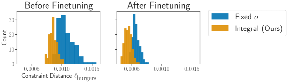
Figure 8: Fixed $\sigma$ vs. integrating over $[0,\sigma_{\text{max}}]$. The NAMM objective involves optimizing $\mathbf{f}_{\psi}$ over the sequence of noisy mirror distributions defined in Eq. 2. We compare this approach of integrating over $\sigma\in[0,\sigma_{\text{max}}]$ to setting a fixed noise std. dev. $\sigma=\sigma_{\text{max}}$ in the context of the 1D Burgers’ constraint (here $\sigma_{\text{max}}=0.1$). Both before and after finetuning, the constraint distances $\ell_{\text{burgers}}$ of inverted MDM samples are smaller if the NAMM was trained with varying $\sigma$. The histograms show the constraint distances of $128$ samples from each method.

A.3 Data assimilation with mirror DPS

Following the original DPS [17], we use a measurement-weight hyperparameter $\zeta\in\mathbb{R}_{>0}$ to re-weight the time-dependent measurement likelihood. At diffusion time $t$, the measurement weight is given by

$$\zeta(t):=\zeta/\left\lVert\mathbf{y}-\mathbf{\mathcal{A}}(\hat{\mathbf{x}}_{0})\right\rVert_{\mathbf{\Gamma}},$$ (8)

where $\hat{\mathbf{x}}_{0}:=\mathbf{f}_{\psi}\left(\mathbb{E}[\tilde{\mathbf{x}}(0)\mid\tilde{\mathbf{x}}(t)]\right)$. Here we assume that the measurement process has the form

$$\mathbf{y}=\mathbf{\mathcal{A}}(\mathbf{x}^{*})+\mathbf{n},\quad\mathbf{n}\sim\mathcal{N}(\mathbf{0}_{m},\mathbf{\Gamma})$$ (9)

for some unknown source image $\mathbf{x}^{*}\in\mathbb{R}^{d}$, where $\mathbf{\mathcal{A}}:\mathbb{R}^{d}\to\mathbb{R}^{m}$ is a known forward operator, and $m\times m$ is the known noise covariance matrix $\mathbf{\Gamma}$. Higher values of $\zeta$ impose greater measurement consistency, but setting $\zeta$ too high can cause instabilities and artifacts. The data assimilation results in Fig. 5 used $\zeta=0.1$ and constraint-guidance weight equal to $200$. Fig. 9 shows results for the same tasks but different values of $\zeta$ in DPS and the constraint-guidance weight in CG-DPS.

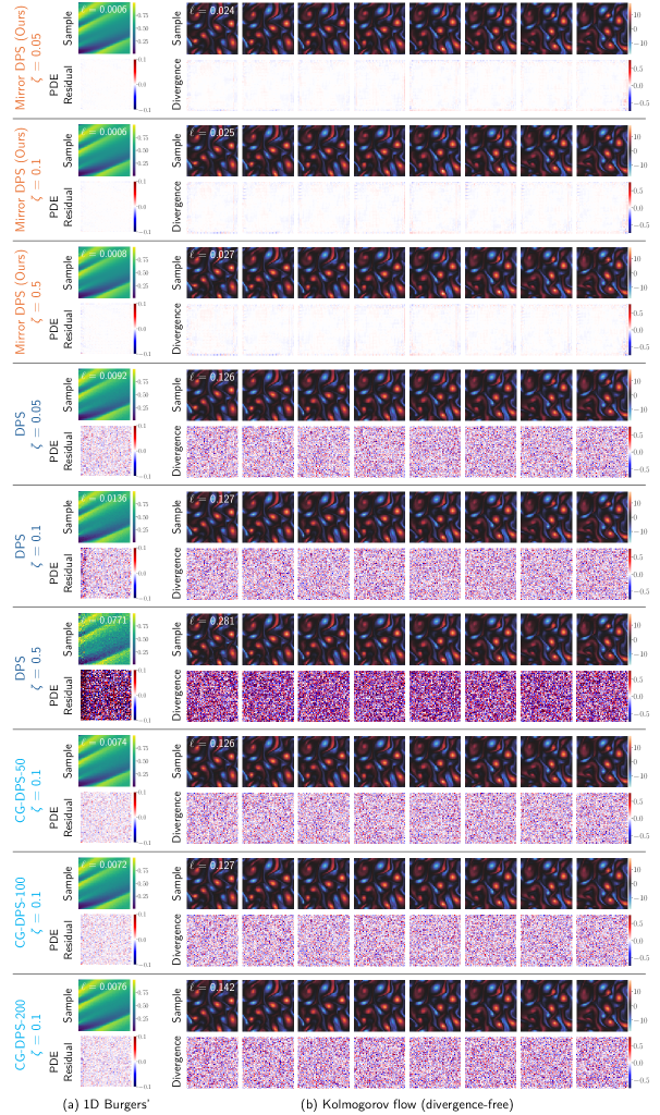
Figure 9: Data assimilation results for different values of $\zeta$ and constraint-guidance strengths. E.g., “CG-DPS-50” refers to CG-DPS with a constraint-guidance weight of $50$. These highlight that even for different values of $\zeta$, the constraint errors (i.e., PDE residual or absolute divergence) of our solutions are much smaller than those of the baseline solutions. Furthermore, changing the constraint-guidance weight of CG-DPS does not meaningfully change the level of constraint satisfaction.

Appendix B Constraint details

Here we provide details about each demonstrated constraint and its corresponding dataset.

Total brightness

The total brightness, or flux, of a discrete image $\mathbf{x}\in\mathbb{R}^{d}$ is simply the sum of its pixel values: $V(\mathbf{x}):=\sum_{i=1}^{d}\mathbf{x}_{i}$. We use the constraint distance function

$$\ell_{\text{flux}}(\mathbf{x}):=\left\lvert V(\mathbf{x})-\bar{V}\right\rvert,$$

where $\bar{V}\in\mathbb{R}_{\geq 0}$ is the target total brightness. The dataset used for this constraint contains images from general relativistic magneto-hydrodynamic (GRMHD) simulations [68] of SgrA* with a fixed field of view. The images (originally $400\times 400$) were resized to $64\times 64$ pixels and rescaled to have a total flux of $120$. The dataset consists of $100000$ training images and $100$ validation images.

1D Burgers’

Burgers’ equation [7, 13] is a nonlinear PDE that is a useful model for fluid mechanics. We consider the equation for a viscous fluid $u=u(t,x)$ in one-dimensional space:

$$\frac{\partial u}{\partial t}+u\frac{\partial u}{\partial x} =\nu\frac{\partial^{2}u}{\partial x^{2}},$$ (10)

where $u(0,x)$ is some initial condition $u_{0}(x)$, and $\nu\in\mathbb{R}_{\geq 0}$ is the viscosity coefficient. We use Crank-Nicolson [19] to discretize and approximately solve Eq. 10 by representing the solution on an $n_{x}\times n_{t}$ grid, where $n_{x}$ is the spatial discretization, and $n_{t}$ is the number of snapshots in time. Given an $n_{x}\times n_{t}$ image, we wish to verify that it could be a solution to Eq. 10 with the Crank-Nicolson discretization. Letting $\mathbf{x}\in\mathbb{R}^{n_{x}\times n_{t}}$ denote the 2D image, we formulate the following distance function for evaluating agreement with the Crank-Nicolson solver:

$$\ell_{\text{burgers}}(\mathbf{x}):=\frac{1}{n_{t}-1}\sum_{t=0}^{n_{t}-2}\left\lVert\mathbf{x}[:,t+1]-f_{\text{C-N}}(\mathbf{x}[:,t])\right\rVert_{1},$$

where $f_{\text{C-N}}:\mathbb{R}^{n_{x}}\to\mathbb{R}^{n_{x}}$ outputs the snapshot at the next time using Crank-Nicolson, and Pythonic notation is used for simplicity. Note that a finite-differences loss à la physics-informed neural networks (PINNs) [54] would also work, but then our data would have non-negligible constraint distances since Crank-Nicolson solutions do not strictly follow a low-order finite-differences approximation.

Using a Crank-Nicolson solver [19] implemented with Diffrax [41], we numerically solved the 1D Burgers’ equation (Eq. 10) with viscosity coefficient $\nu=0.5$. The initial conditions were sampled from a Gaussian process based on a Matérn kernel with smoothness parameter $1.5$ and length scale equal to $1.0$. We discretized the spatiotemporal domain into a $64\times 64$ grid covering the spatial extent $x\in[0,10]$ and time interval $t\in[0,8]$. We ran Crank-Nicolson with a time step of $\Delta t=0.025$ and saved every fifth step for a total of $64$ snapshots. We followed this process to create our 1D Burgers’ dataset of $10000$ training images and $1000$ validation images.

Divergence-free

The study of fluid dynamics often involves incompressible, or divergence-free, fluids. Letting $\mathbf{u}=\mathbf{u}(x,y,t)$ be the time-dependent trajectory of a 2D velocity field, the divergence-free constraint says that $\nabla\cdot\mathbf{u}=\frac{\partial\mathbf{u}_{x}}{\partial x}+\frac{\partial\mathbf{u}_{y}}{\partial y}=0$. We assume an $n_{x}\times n_{y}$ spatial grid and represent trajectories as two-channel (for the two velocity components) images showing each $n_{x}\times n_{y}$ snapshot for a total of $n_{t}$ snapshots. Such an image $\mathbf{x}$ has a corresponding image of the divergence field $\text{div}(\mathbf{x})$, which has the same size as $\mathbf{x}$ and represents the divergence of the trajectory. We formulate the following distance function that penalizes non-zero divergence:

$$\ell_{\text{div}}(\mathbf{x}):=\left\lVert\text{div}(\mathbf{x})\right\rVert_{1}.$$

We created a dataset of Kolmogorov flows, which satisfy a Navier-Stokes PDE, to demonstrate the divergence-free constraint. The Navier-Stokes PDEs are ubiquitous in fields including fluid dynamics, mathematics, and climate modeling and have the following form:

$$\frac{\partial\mathbf{u}}{\partial t}=-\mathbf{u}\nabla\mathbf{u}+\frac{1}{Re}\nabla^{2}\mathbf{u}-\frac{1}{\rho}\nabla p+\mathbf{f}\\ \nabla\cdot\mathbf{u}=0,$$

where $\mathbf{u}=\mathbf{u}(x,y,t)$ is the 2D velocity field at spatial location $(x,y)$ and time $t$, $Re$ is the Reynolds number, $\rho$ is the density, $p$ is the pressure field, and $\mathbf{f}$ is the external forcing. Following Kochkov et al. [44] and Rozet and Louppe [56], we set $Re=10^{3}$, $\rho=1$, and $\mathbf{f}$ corresponding to Kolmogorov forcing [14, 10] with linear damping. We consider the spatial domain $[0,2\pi]^{2}$ with periodic boundary conditions and discretize it into a $64\times 64$ uniform grid. We used jax-cfd [44] to randomly sample divergence-free, spectrally filtered initial conditions and then solve the Navier-Stokes equations with the forward Euler integration method with $\Delta t=0.01$ time units. We saved a snapshot every $20$ time units for a total of $8$ snapshots in the time interval $[3,4.6]$. We represent the solution as a two-channel $128\times 256$ image showing the snapshots in left-to-right order. In total, the dataset consists of $10000$ training images and $1000$ validation images.

Periodic

Assuming the constraint that every image is a periodic tiling of $n_{\text{tiles}}$ unit cells, we formulate the following constraint distance for a given image $\mathbf{x}$:

$$\ell_{\text{periodic}}(\mathbf{x}):=\sum_{i=1}^{n_{\text{tiles}}}\frac{1}{n_{\text{tiles}}}\sum_{j=1}^{n_{\text{tiles}}}\left\lVert\mathbf{t}_{i}(\mathbf{x})-\mathbf{t}_{j}(\mathbf{x})\right\rVert_{1},$$

which compares each pair of tiles, where $\mathbf{t}_{i}(\mathbf{x})$ denotes the $i$-th tile in the image. For our experiments, we consider $32\times 32$ unit cells that are tiled in a $2\times 2$ pattern to create $64\times 64$ images. Using the unit-cell generation code of Ogren et al. [52], we created a dataset of $30000$ training images and $300$ validation images.

Count

For the count constraint, we rely on a CNN to estimate the count of a particular object. Letting $f_{\text{CNN}}:\mathbb{R}^{d}\to\mathbb{R}$ be the trained counting CNN, we turn to the following constraint distance function for a target count $\bar{c}$:

$$\ell_{\text{count}}(\mathbf{x}):=\left\lvert f_{\text{CNN}}(\mathbf{x})-\bar{c}\right\rvert.$$

We demonstrate this constraint with astronomical images that contain a certain number of galaxies. In particular, we simulated $128\times 128$ images of radio galaxies with background noise [18], each of which has exactly eight ($\bar{c}=8$) galaxies with an SNR $\geq 15$ dB. The dataset consists of $10000$ training images and $1000$ validation images.

To train the counting CNN, we created a mixed dataset with images of $6,7,8,9,$ or $10$ galaxies that includes $10000$ training images and $1000$ validation images for each of the five labels. The CNN architecture was adapted from a simple MNIST classifier [1] with two convolutional layers followed by two dense layers with ReLU activations. The CNN was trained to minimize the mean squared error between the real-valued estimated count and the ground-truth count.

References

- 8bitmp3 [2023] 8bitmp3. Jax-flax-tutorial-image-classification-with-linen. https://github.com/8bitmp3/JAX-Flax-Tutorial-Image-Classification-with-Linen, 2023.
- Alfano et al. [2024] Carlo Alfano, Sebastian Towers, Silvia Sapora, Chris Lu, and Patrick Rebeschini. Meta-learning the mirror map in policy mirror descent. arXiv preprint arXiv:2402.05187, 2024.
- Allingham et al. [2022] James Urquhart Allingham, Javier Antoran, Shreyas Padhy, Eric Nalisnick, and José Miguel Hernández-Lobato. Learning generative models with invariance to symmetries. In NeurIPS 2022 Workshop on Symmetry and Geometry in Neural Representations, 2022.
- Amos et al. [2017] Brandon Amos, Lei Xu, and J Zico Kolter. Input convex neural networks. In International Conference on Machine Learning, pages 146–155. PMLR, 2017.
- Anderson [1982] Brian DO Anderson. Reverse-time diffusion equation models. Stochastic Processes and their Applications, 12(3):313–326, 1982.
- Bansal et al. [2023] Arpit Bansal, Hong-Min Chu, Avi Schwarzschild, Soumyadip Sengupta, Micah Goldblum, Jonas Geiping, and Tom Goldstein. Universal guidance for diffusion models. In Proceedings of the IEEE/CVF Conference on Computer Vision and Pattern Recognition, pages 843–852, 2023.
- Bateman [1915] Harry Bateman. Some recent researches on the motion of fluids. Monthly Weather Review, 43(4):163–170, 1915.
- Batzner et al. [2022] Simon Batzner, Albert Musaelian, Lixin Sun, Mario Geiger, Jonathan P Mailoa, Mordechai Kornbluth, Nicola Molinari, Tess E Smidt, and Boris Kozinsky. E (3)-equivariant graph neural networks for data-efficient and accurate interatomic potentials. Nature communications, 13(1):2453, 2022.
- Beck and Teboulle [2003] Amir Beck and Marc Teboulle. Mirror descent and nonlinear projected subgradient methods for convex optimization. Operations Research Letters, 31(3):167–175, 2003.
- Boffetta and Ecke [2012] Guido Boffetta and Robert E Ecke. Two-dimensional turbulence. Annual review of fluid mechanics, 44:427–451, 2012.
- Boyda et al. [2021] Denis Boyda, Gurtej Kanwar, Sébastien Racanière, Danilo Jimenez Rezende, Michael S Albergo, Kyle Cranmer, Daniel C Hackett, and Phiala E Shanahan. Sampling using su (n) gauge equivariant flows. Physical Review D, 103(7):074504, 2021.
- Bubeck et al. [2015] Sébastien Bubeck et al. Convex optimization: Algorithms and complexity. Foundations and Trends® in Machine Learning, 8(3-4):231–357, 2015.
- Burgers [1948] Johannes Martinus Burgers. A mathematical model illustrating the theory of turbulence. Advances in applied mechanics, 1:171–199, 1948.
- Chandler and Kerswell [2013] Gary J Chandler and Rich R Kerswell. Invariant recurrent solutions embedded in a turbulent two-dimensional kolmogorov flow. Journal of Fluid Mechanics, 722:554–595, 2013.
- Chang et al. [2007] Ming-Wei Chang, Lev Ratinov, and Dan Roth. Guiding semi-supervision with constraint-driven learning. In Proceedings of the 45th annual meeting of the association of computational linguistics, pages 280–287, 2007.
- Choi et al. [2021] Jooyoung Choi, Sungwon Kim, Yonghyun Jeong, Youngjune Gwon, and Sungroh Yoon. Ilvr: Conditioning method for denoising diffusion probabilistic models. In ICCV. IEEE, 2021.
- Chung et al. [2022] Hyungjin Chung, Jeongsol Kim, Michael T Mccann, Marc L Klasky, and Jong Chul Ye. Diffusion posterior sampling for general noisy inverse problems. arXiv preprint arXiv:2209.14687, 2022.
- Connor et al. [2022] Liam Connor, Katherine L Bouman, Vikram Ravi, and Gregg Hallinan. Deep radio-interferometric imaging with polish: Dsa-2000 and weak lensing. Monthly Notices of the Royal Astronomical Society, 514(2):2614–2626, 2022.
- Crank and Nicolson [1947] John Crank and Phyllis Nicolson. A practical method for numerical evaluation of solutions of partial differential equations of the heat-conduction type. In Mathematical proceedings of the Cambridge philosophical society, volume 43, pages 50–67. Cambridge University Press, 1947.
- Daras et al. [2024] Giannis Daras, Yuval Dagan, Alex Dimakis, and Constantinos Daskalakis. Consistent diffusion models: Mitigating sampling drift by learning to be consistent. Advances in Neural Information Processing Systems, 36, 2024.
- De Bortoli et al. [2022] Valentin De Bortoli, Emile Mathieu, Michael Hutchinson, James Thornton, Yee Whye Teh, and Arnaud Doucet. Riemannian score-based generative modelling. Advances in Neural Information Processing Systems, 35:2406–2422, 2022.
- Dey et al. [2020] Neel Dey, Antong Chen, and Soheil Ghafurian. Group equivariant generative adversarial networks. arXiv preprint arXiv:2005.01683, 2020.
- Efron [2011] Bradley Efron. Tweedie’s formula and selection bias. Journal of the American Statistical Association, 106(496):1602–1614, 2011.
- et al. [2019] The Event Horizon Telescope Collaboration et al. First m87 event horizon telescope results. iv. imaging the central supermassive black hole. The Astrophysical Journal Letters, 875(1):L4, apr 2019. doi: 10.3847/2041-8213/ab0e85. URL https://dx.doi.org/10.3847/2041-8213/ab0e85.
- et al. [2022] The Event Horizon Telescope Collaboration et al. First sagittarius a* event horizon telescope results. iii. imaging of the galactic center supermassive black hole. The Astrophysical Journal Letters, 930(2):L14, may 2022. doi: 10.3847/2041-8213/ac6429. URL https://dx.doi.org/10.3847/2041-8213/ac6429.
- Fishman et al. [2023a] Nic Fishman, Leo Klarner, Valentin De Bortoli, Emile Mathieu, and Michael Hutchinson. Diffusion models for constrained domains. arXiv preprint arXiv:2304.05364, 2023a.
- Fishman et al. [2023b] Nic Fishman, Leo Klarner, Emile Mathieu, Michael Hutchinson, and Valentin De Bortoli. Metropolis sampling for constrained diffusion models. Advances in Neural Information Processing Systems, 36, 2023b.
- Ganchev et al. [2010] Kuzman Ganchev, Joao Graça, Jennifer Gillenwater, and Ben Taskar. Posterior regularization for structured latent variable models. The Journal of Machine Learning Research, 11:2001–2049, 2010.
- Garcia Satorras et al. [2021] Victor Garcia Satorras, Emiel Hoogeboom, Fabian Fuchs, Ingmar Posner, and Max Welling. E (n) equivariant normalizing flows. Advances in Neural Information Processing Systems, 34:4181–4192, 2021.
- Geiger and Smidt [2022] Mario Geiger and Tess Smidt. e3nn: Euclidean neural networks. arXiv preprint arXiv:2207.09453, 2022.
- Giannone et al. [2023] Giorgio Giannone, Lyle Regenwetter, Akash Srivastava, Dan Gutfreund, and Faez Ahmed. Learning from invalid data: On constraint satisfaction in generative models. arXiv preprint arXiv:2306.15166, 2023.
- Graikos et al. [2022] Alexandros Graikos, Nikolay Malkin, Nebojsa Jojic, and Dimitris Samaras. Diffusion models as plug-and-play priors. Advances in Neural Information Processing Systems, 35:14715–14728, 2022.
- Ho et al. [2020] Jonathan Ho, Ajay Jain, and Pieter Abbeel. Denoising diffusion probabilistic models. Advances in Neural Information Processing Systems, 33:6840–6851, 2020.
- Hoogeboom et al. [2022] Emiel Hoogeboom, Vıctor Garcia Satorras, Clément Vignac, and Max Welling. Equivariant diffusion for molecule generation in 3d. In International conference on machine learning, pages 8867–8887. PMLR, 2022.
- Hsieh et al. [2018] Ya-Ping Hsieh, Ali Kavis, Paul Rolland, and Volkan Cevher. Mirrored langevin dynamics. Advances in Neural Information Processing Systems, 31, 2018.
- Huang et al. [2022] Chin-Wei Huang, Milad Aghajohari, Joey Bose, Prakash Panangaden, and Aaron C Courville. Riemannian diffusion models. Advances in Neural Information Processing Systems, 35:2750–2761, 2022.
- Huang et al. [2024] Yujia Huang, Adishree Ghatare, Yuanzhe Liu, Ziniu Hu, Qinsheng Zhang, Chandramouli S Sastry, Siddharth Gururani, Sageev Oore, and Yisong Yue. Symbolic music generation with non-differentiable rule guided diffusion. arXiv preprint arXiv:2402.14285, 2024.
- Hyvärinen and Dayan [2005] Aapo Hyvärinen and Peter Dayan. Estimation of non-normalized statistical models by score matching. Journal of Machine Learning Research, 6(4), 2005.
- Jalal et al. [2021] Ajil Jalal, Marius Arvinte, Giannis Daras, Eric Price, Alexandros G Dimakis, and Jonathan I Tamir. Robust compressed sensing mri with deep generative priors. NeurIPS, 2021.
- Kawar et al. [2022] Bahjat Kawar, Michael Elad, Stefano Ermon, and Jiaming Song. Denoising diffusion restoration models. In Advances in Neural Information Processing Systems, 2022.
- Kidger [2022] Patrick Kidger. On neural differential equations. arXiv preprint arXiv:2202.02435, 2022.
- Kingma et al. [2021] Diederik P. Kingma, Tim Salimans, Ben Poole, and Jonathan Ho. Variational diffusion models. arXiv preprint arXiv:2107.00630, 2021.
- Klein et al. [2024] Leon Klein, Andreas Krämer, and Frank Noé. Equivariant flow matching. Advances in Neural Information Processing Systems, 36, 2024.
- Kochkov et al. [2021] Dmitrii Kochkov, Jamie A Smith, Ayya Alieva, Qing Wang, Michael P Brenner, and Stephan Hoyer. Machine learning–accelerated computational fluid dynamics. Proceedings of the National Academy of Sciences, 118(21):e2101784118, 2021.
- Köhler et al. [2020] Jonas Köhler, Leon Klein, and Frank Noé. Equivariant flows: exact likelihood generative learning for symmetric densities. In International conference on machine learning, pages 5361–5370. PMLR, 2020.
- Li et al. [2022] Ruilin Li, Molei Tao, Santosh S Vempala, and Andre Wibisono. The mirror langevin algorithm converges with vanishing bias. In International Conference on Algorithmic Learning Theory, pages 718–742. PMLR, 2022.
- Liu et al. [2024] Guan-Horng Liu, Tianrong Chen, Evangelos Theodorou, and Molei Tao. Mirror diffusion models for constrained and watermarked generation. Advances in Neural Information Processing Systems, 36, 2024.
- Lou and Ermon [2023] Aaron Lou and Stefano Ermon. Reflected diffusion models. ICML, 2023.
- Mann and McCallum [2007] Gideon S Mann and Andrew McCallum. Simple, robust, scalable semi-supervised learning via expectation regularization. In Proceedings of the 24th international conference on Machine learning, pages 593–600, 2007.
- Midgley et al. [2024] Laurence Midgley, Vincent Stimper, Javier Antorán, Emile Mathieu, Bernhard Schölkopf, and José Miguel Hernández-Lobato. Se (3) equivariant augmented coupling flows. Advances in Neural Information Processing Systems, 36, 2024.
- Niu et al. [2020] Chenhao Niu, Yang Song, Jiaming Song, Shengjia Zhao, Aditya Grover, and Stefano Ermon. Permutation invariant graph generation via score-based generative modeling. In International Conference on Artificial Intelligence and Statistics, pages 4474–4484. PMLR, 2020.
- Ogren et al. [2024] Alexander C Ogren, Berthy T Feng, Katherine L Bouman, and Chiara Daraio. Gaussian process regression as a surrogate model for the computation of dispersion relations. Computer Methods in Applied Mechanics and Engineering, 420:116661, 2024.
- Paiss et al. [2023] Roni Paiss, Ariel Ephrat, Omer Tov, Shiran Zada, Inbar Mosseri, Michal Irani, and Tali Dekel. Teaching clip to count to ten. In Proceedings of the IEEE/CVF International Conference on Computer Vision, pages 3170–3180, 2023.
- Raissi et al. [2019] Maziar Raissi, Paris Perdikaris, and George E Karniadakis. Physics-informed neural networks: A deep learning framework for solving forward and inverse problems involving nonlinear partial differential equations. Journal of Computational Physics, 378:686–707, 2019.
- Rezende et al. [2019] Danilo Jimenez Rezende, Sébastien Racanière, Irina Higgins, and Peter Toth. Equivariant hamiltonian flows. arXiv preprint arXiv:1909.13739, 2019.
- Rozet and Louppe [2024] François Rozet and Gilles Louppe. Score-based data assimilation. Advances in Neural Information Processing Systems, 36, 2024.
- Satorras et al. [2021] Vıctor Garcia Satorras, Emiel Hoogeboom, and Max Welling. E (n) equivariant graph neural networks. In International conference on machine learning, pages 9323–9332. PMLR, 2021.
- Sohl-Dickstein et al. [2015] Jascha Sohl-Dickstein, Eric Weiss, Niru Maheswaranathan, and Surya Ganguli. Deep unsupervised learning using nonequilibrium thermodynamics. In Int. Conf. Machine Learning, pages 2256–2265. PMLR, 2015.
- Song et al. [2023] Jiaming Song, Arash Vahdat, Morteza Mardani, and Jan Kautz. Pseudoinverse-guided diffusion models for inverse problems. In International Conference on Learning Representations, 2023. URL https://openreview.net/forum?id=9_gsMA8MRKQ.
- Song and Ermon [2019] Yang Song and Stefano Ermon. Generative modeling by estimating gradients of the data distribution. In NeurIPS, pages 11895–11907, 2019.
- Song et al. [2021a] Yang Song, Conor Durkan, Iain Murray, and Stefano Ermon. Maximum likelihood training of score-based diffusion models. Advances in neural information processing systems, 34:1415–1428, 2021a.
- Song et al. [2021b] Yang Song, Jascha Sohl-Dickstein, Diederik P Kingma, Abhishek Kumar, Stefano Ermon, and Ben Poole. Score-based generative modeling through stochastic differential equations. In ICLR, 2021b. URL https://openreview.net/forum?id=PxTIG12RRHS.
- Song et al. [2022] Yang Song, Liyue Shen, Lei Xing, and Stefano Ermon. Solving inverse problems in medical imaging with score-based generative models. In ICLR, 2022. URL https://openreview.net/forum?id=vaRCHVj0uGI.
- Song et al. [2024] Yuxuan Song, Jingjing Gong, Minkai Xu, Ziyao Cao, Yanyan Lan, Stefano Ermon, Hao Zhou, and Wei-Ying Ma. Equivariant flow matching with hybrid probability transport for 3d molecule generation. Advances in Neural Information Processing Systems, 36, 2024.
- Tan et al. [2023] Hong Ye Tan, Subhadip Mukherjee, Junqi Tang, and Carola-Bibiane Schönlieb. Data-driven mirror descent with input-convex neural networks. SIAM Journal on Mathematics of Data Science, 5(2):558–587, 2023.
- Thomas et al. [2018] Nathaniel Thomas, Tess Smidt, Steven Kearnes, Lusann Yang, Li Li, Kai Kohlhoff, and Patrick Riley. Tensor field networks: Rotation-and translation-equivariant neural networks for 3d point clouds. arXiv preprint arXiv:1802.08219, 2018.
- Vincent [2011] Pascal Vincent. A connection between score matching and denoising autoencoders. Neural computation, 23(7):1661–1674, 2011.
- Wong et al. [2022] George N Wong, Ben S Prather, Vedant Dhruv, Benjamin R Ryan, Monika Mościbrodzka, Chi-kwan Chan, Abhishek V Joshi, Ricardo Yarza, Angelo Ricarte, Hotaka Shiokawa, et al. Patoka: Simulating electromagnetic observables of black hole accretion. The Astrophysical Journal Supplement Series, 259(2):64, 2022.
- Xu et al. [2022] Minkai Xu, Lantao Yu, Yang Song, Chence Shi, Stefano Ermon, and Jian Tang. Geodiff: A geometric diffusion model for molecular conformation generation. arXiv preprint arXiv:2203.02923, 2022.
- Yim et al. [2023] Jason Yim, Brian L Trippe, Valentin De Bortoli, Emile Mathieu, Arnaud Doucet, Regina Barzilay, and Tommi Jaakkola. Se (3) diffusion model with application to protein backbone generation. arXiv preprint arXiv:2302.02277, 2023.
- Zhang et al. [2023] Lvmin Zhang, Anyi Rao, and Maneesh Agrawala. Adding conditional control to text-to-image diffusion models. In Proceedings of the IEEE/CVF International Conference on Computer Vision, pages 3836–3847, 2023.
- Zhou [2018] Xingyu Zhou. On the fenchel duality between strong convexity and lipschitz continuous gradient. arXiv preprint arXiv:1803.06573, 2018.
- Zhu et al. [2017] Jun-Yan Zhu, Taesung Park, Phillip Isola, and Alexei A Efros. Unpaired image-to-image translation using cycle-consistent adversarial networks. In Proceedings of the IEEE international conference on computer vision, pages 2223–2232, 2017.