GA-NIFS: JWST/NIRSpec IFS view of the $z\sim 3.5$ galaxy GS5001 and
its close environment at the core of a large-scale overdensity

We present JWST Near-Infrared Spectrograph (NIRSpec) observations in Integral Field Spectroscopic (IFS) mode of the galaxy GS5001 at redshift z=3.47, the brightest member of a candidate protocluster in the GOODS-S field. The data cover a field of view (FoV) of $4\arcsec\times 4\arcsec$ ($\sim 30\times 30$ kpc²) and were obtained as part of the Galaxy Assembly with NIRSpec IFS (GA-NIFS) GTO program.

The observations include both high (R$\sim$2700) and low (R$\sim$100) spectral resolution data, spanning the rest-frame wavelength ranges 3700-6780 Å and 1300-11850 Å, respectively. These observations enable the detection and mapping of the main optical emission lines from [O ii]$\lambda\lambda 3726,29$ to [S iii]$\lambda 9531$. We analyse the spatially resolved ionised gas kinematics and interstellar medium properties, including obscuration, gas metallicity, excitation, ionisation parameter, and electron density. In addition to the central galaxy, the NIRSpec FoV covers three components in the south (corresponding to the source GS4921, previously identified by HST imaging), with velocities blue-shifted by $\sim-150$ km s^-1 with respect to the main galaxy, and another source in the north redshifted by $\sim 200$ km s^-1. The emission line ratios in the BPT diagram are consistent with star formation for all the sources in the FoV. We measure electron densities of $\sim 500$ cm^-3 in the different sources. The gas-phase metallicity in the main galaxy is 12+log(O/H) $=8.45\pm 0.04$, and slightly lower in the companions (12+log(O/H)$=8.34-8.42$), consistent with the mass-metallicity relation at $z\sim 3$. We find peculiar line ratios (high $\log$[N ii]/H$\alpha$$=[-0.45,-0.3]$, low $\log$[O iii]/H$\beta$$=[0.06,0.10]$) in the northern part of the main galaxy (GS5001). These could be attributed to either higher metallicity, or to shocks resulting from the interaction of the main galaxy with the northern source. We identify a spatially resolved outflow in the main galaxy, traced by a broad symmetric component in H$\alpha$ and [O iii], with an extension of about 3 kpc. We find maximum outflow velocities of $\sim 400$ km s^-1, an outflow mass of $(1.7\pm 0.4)\times 10^{8}$ M_⊙, a mass outflow rate of $23\pm 5$ M_⊙ yr^-1and a mass loading factor of 0.23. These properties are compatible with star formation being the driver of the outflow. Our analysis of these JWST NIRSpec IFS data therefore provides valuable, unprecedented insights into the interplay between star formation, galactic outflows and interactions in the core of a $z\sim 3.5$ candidate protocluster.

1 Introduction

Understanding the complex processes governing galaxy formation and evolution in the early Universe requires detailed observations of their interstellar medium (ISM) properties and kinematics. Several studied have investigated how the ISM properties evolve with time, focusing for instance on the ionisation parameter, electron density and temperature, and metallicity (e.g. Nakajima & Ouchi, 2014; Kaasinen et al., 2017, 2018; Curti et al., 2024; Reddy et al., 2023a, b; Sanders et al., 2016, 2021, 2024).

Spatially resolved studies of low- and intermediate-redshift ($z<3$) galaxies have found spatial variations of these properties within galaxies (e.g. Cresci et al., 2010; Troncoso et al., 2014; Stott et al., 2016; Curti et al., 2020a; Gillman et al., 2022). These studies highlighted the importance of resolving the inner structure of the ISM properties in order to understand galaxy evolution. Spatially resolved observations of optical emission lines allowed the study of the internal kinematics of galaxies up to high-redshift (e.g. Wisnioski et al., 2015, 2019; Harrison et al., 2016, 2017; Förster Schreiber et al., 2018; Förster Schreiber & Wuyts, 2020; van Houdt et al., 2021; Übler et al., 2024a). These studies have also identified and characterised outflows powered by active galactic nuclei or star-bursts (e.g. Förster Schreiber et al., 2014, 2019). At cosmic noon ($z=1-2$), these types of studies have been performed using ground-based facilities with NIR integral field spectroscopy (IFS) instruments. However, from the ground the H$\alpha$ line can only be observed up to $z\sim 2.5$ and H$\beta$+[O iii] up to $z\sim 3.5$.

The IFS capabilities of the NIRSpec instrument (Jakobsen et al., 2022; Böker et al., 2022) on board the James Webb Space Telescope (JWST) enable for the first time to map the optical lines at $z>3$ with a spatial resolution $\sim 0.1$”. Several works have demonstrated the capability of JWST/NIRSpec integral field units to study the ISM properties and gas kinematics in star-forming galaxies and active galactic nuclei (AGN) host galaxies at $z>3$ (e.g. Wylezalek et al., 2022; Übler et al., 2023, 2024b; Perna et al., 2023; Parlanti et al., 2024; Vayner et al., 2024; Wang et al., 2024; Roy et al., 2024; Saxena et al., 2024).

In this work, we present JWST/NIRSpec IFS observation of the galaxy GS5001 and its close companions. GS5001 (also known as Candels-5001 and as ID 4417 in the GOODS-MUSIC catalog, Grazian et al., 2006) is a Lyman-break selected galaxy in the GOODS-S field at z=3.473 (Maiolino et al., 2008) at coordinates R.A.= 03:32:23.35, Dec = -27:51:57.13. Two other galaxies detected in the HST/UV images lie in close projected separation (1-2$\arcsec$, 7-15 kpc): GS4921 to the south (ID 4414 in the GOODS-MUSIC catalog) and GS4923 to the north (see central panel in Fig. 1). GS4921 was confirmed to be at a similar redshift ($z=3.471$), based on VLT/SINFONI observations (Maiolino et al., 2008). GS4923 has a photometric redshift of 0.2 (Pérez-González et al., 2005), but some [O iii] emission at a similar redshift of 3.47 was tentatively identified at its location using VLT/SINFONI data (Ginolfi et al., 2017).

GS5001 is the brightest member of a system classified as a candidate protocluster, as it lies in a large-scale overdensity of galaxies (Franck & McGaugh, 2016). Ginolfi et al. (2017) detect a large reservoir of molecular gas, traced by CO(4–3), which extends up to 40 kpc around this system. Additionally, they detect several CO(4–3) emitting systems within a radius of 250 kpc, mostly distributed along the same NE-SW direction as the CO(4–3) reservoir (see their Fig. 9); they suggest that these systems are tracing the inner and densest regions of a large-scale accreting stream feeding the central massive galaxy GS5001.

GS5001 has a star-formation rate (SFR) in the range 150-240 M_⊙ yr^-1 (Troncoso et al., 2014; Pacifici et al., 2016; Pérez-González et al., 2005; Guo et al., 2013), derived from spectral energy distribution (SED) fitting of the UV to FIR photometry, and a stellar mass in the range $M_{\star}=1-4\times 10^{10}$ M_⊙ (Maiolino et al., 2008; Pérez-González et al., 2005; Guo et al., 2013; Santini et al., 2015; Pacifici et al., 2016). The southern companion, GS4921, has SFR = $35-70$ M_⊙ yr^-1 and stellar mass $M_{\star}=0.5-2.3\times 10^{10}$ M_⊙ (Maiolino et al., 2008; Pérez-González et al., 2005; Guo et al., 2013). All values reported here have been homogenised to a Chabrier (2003) IMF. GS5001 is also detected in the X-ray, although with a small number of counts (20 counts), and has an aperture corrected X-ray luminosity of $L_{0.5-7\,\mathrm{keV}}=9.5\times 10^{42}$ erg s^-1 (Fiore et al., 2012; Luo et al., 2017). Despite the high X-ray luminosity, it is not clear whether this object hosts an AGN, because its very high SFR could be responsible for most of the X-ray flux (Fiore et al., 2012).

The goal of this work is the detailed characterisation of the physical and kinematic properties of GS5001 and its close environment. Other recent studies characterising dense environments in the early universe using JWST/NIRSpec IFS include those by Perna et al. (2023, LBQS 0302-0019; a dual AGN with multiple companions at $z\sim 3.3$), Rodríguez Del Pino et al. (2024, GS4891; a galaxy group at $z\sim 3.7$), Jones et al. (2024a, HZ10; a galaxy group at $z\sim 5.7$), Jones et al. (2024b, HFLS3; an overdensity at $z\sim 6.3$), and Arribas et al. (2023, SPT0311-58; a protocluster core at $z\sim 6.9$). This paper is organised as follows. Section 2 presents the JWST/NIRSpec observations and the data reduction. In Section 3 we describe the method used for the emission line fitting. In Section 4 we present the results. First, we show the ionised gas kinematics (Sec. 4.2) and then the properties of the ISM (attenuation, BPT, metallicity, ionisation parameter, electron density, Sec. 4.3). The Discussion is in Section 5 and the Conclusions in Section 6.

Throughout this work, we assume a cosmological model with $\Omega_{\lambda}=0.7$, $\Omega_{\text{M}}=0.3$ , and $H_{0}=70$ km s^-1 Mpc^-1, that results in a scale of 7.34 kpc/arcsec at $z=3.47$. In this work, we assume a Chabrier (2003) initial mass function (IMF).

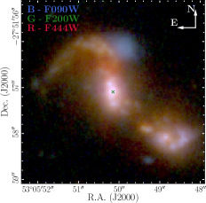
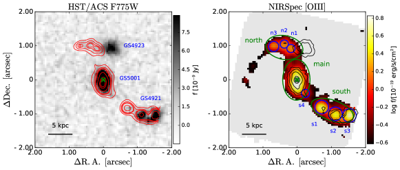
Figure 1: Identification of galaxies and structures around GS5001. Left: NIRCam three-color image of GS5001. Middle: HST/ACS F775W band image with contours of the NIRSpec [O iii] emission in red. In blue are the names of the sources identified in CANDELS. Right: NIRSpec [O iii] flux map with contours of the HST ACS/F775W emission in black. Blue and green regions mark the different components identified in the [O iii] map. The green crosses show the center of the continuum emission in the HST/WFC3 F125W filter, used for astrometric registration.

2 Observations and data reduction

2.1 JWST/NIRSpec observations

We present observations of GS5001 obtained on Dec. 10th 2022 as part of the Galaxy Assembly with NIRSpec Integral Field Spectroscopy (GA-NIFS) GTO program (PIs: S. Arribas, R. Maiolino), contained within program #1216 (PI: N. Lützgendorf). The main goal of GA-NIFS is to study the internal structure and the close environment of a sample of 55 galaxies and AGN at $z=2-11$ (Perna, 2023).

GS5001 was observed with NIRSpec IFS (Böker et al., 2022; Rigby et al., 2023) both with the high-resolution ($R\sim 2700$) and with the low-resolution ($R\sim 100$) mode. The R2700 observations use the grating/filter pair G235H/F170LP, covering the wavelength range $1.66-3.16$ $\mu$m  with a spectral resolution R$\sim 1900-3500$ (Jakobsen et al., 2022). The R100 PRISM/CLEAR data covers the range $0.6-5.3$ $\mu$m  with R$\sim 30-300$. Both observations were taken using an IRS² detector readout pattern (NRSIRS2 for R2700 and NRSIRS2RAPID for R100; Rauscher et al., 2017), which significantly reduces the detector noise with respect to the standard procedure. The R2700 observations have an exposure time of 4.1 hours, while the R100 observations an exposure time of 1.1 hours. We use an 8-point medium cycling dither pattern, which provides a total observed field of view (FoV) of $\sim 4"\times 4"$ ($\sim 29\times 29$ kpc² at the redshift of the target).

2.2 Data reduction

The raw data were reduced with the JWST calibration pipeline version 1.8.2, using the CRDS context file jwst_1068.pmap. The default reduction pipeline was modified to improve the data quality, as explained in detail in Perna et al. (2023) and D’Eugenio et al. (2023). We build the final cubes with a spaxel size of 0.05” using the ‘drizzle’ method.

For the subtraction of the background emission from the R100 data cube, we extract spectra from spaxels in regions of the FoV where no galaxy emission is present and calculate a median spectrum. Then, we subtract this median spectrum from the data cube. The background subtraction is not needed for the R2700 data, as the background contribution is not significant and it is accounted for during the line fitting procedure. We note that the noise given in the data cube (‘ERR’ extension) is underestimated compared to the actual noise in the data. Therefore, we re-scale the ‘error’ vector in each spaxel by a factor of $1.4-3.1$ (median 1.6) to match the noise estimated from the standard deviation of the continuum in spectral regions free of line emission (following the method used by e.g. Übler et al., 2023; Rodríguez Del Pino et al., 2024). Specifically, we selected the continuum spectral regions $4700-4800$ Å, $5050-5200$ Å, and $6000-6400$ Å (rest-frame wavelength).

Fig. 2 shows the R2700 and R100 spectra extracted from the central $3\times 3$ spaxels of the main galaxy. This figure illustrates the wavelength range spanned by the two spectra, the main emission lines and the quality of the data.

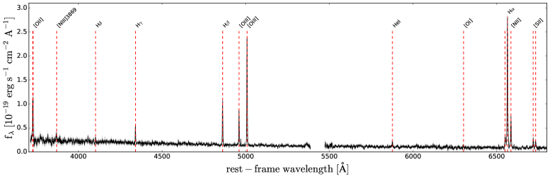
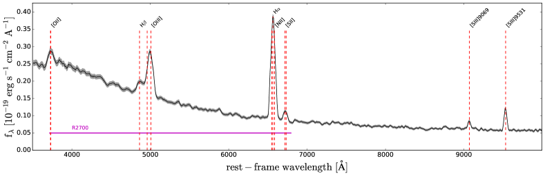
Figure 2: Average rest-frame spectrum of the main galaxy central $3\times 3$ spaxels ($0.15\arcsec\times 0.15\arcsec$), from the high-resolution ($R\sim 2700$, upper) and low-resolution ($R\sim 100$, lower) NIRSpec data. Vertical dashed lines mark the position of the detected emission lines. The grey shaded area shows the error on the fluxes. The magenta line in the lower panel shows the wavelength range covered by the R2700 data.

2.3 Ancillary data

In addition to the NIRSpec data, we also consider other observations of GS5001. In particular, we use images from HST and JWST/NIRCam, and ALMA observations of the CO(4–3) emission line.

The HST/ACS WFC F755W and HST/WFC3 F125W images of GS5001 have been downloaded from the Rainbow Cosmological Survey database. The astrometric alignment is explained in the following section. We also download publicly available JWST/NIRCam images (F090W, F200W, F444W) of GS5001 from the multi-object JWST Deep Extragalactic Survey (JADES; Eisenstein et al., 2023; Rieke et al., 2023). The astrometric alignment of the NIRCam images is described in Rieke et al. (2023).

In this work, we also use ALMA observations of the CO(4–3) emission (project ID 2012.1.00423.S, P.I. T. Nagao), which have been presented in Ginolfi et al. (2017). We obtain the calibrated measurement sets (MS) from the European ALMA Regional Centre (ARC). We create a data cube of the CO(4–3) spectral window using the ALMA data reduction software CASA v6.2.1 (CASA Team et al., 2022). We use the CASA task tclean applying natural weighting to generate a data cube with synthesised beam FWHM $1.9\times 1.3$ arcsec². The CO(4–3) intensity map (moment 0) is produced by integrating the continuum subtracted data cube in the spectral channels within $\pm 800$ km s^-1 from the CO(4–3) emission frequency at $z=3.47$.

2.4 Astrometry

We register the astrometry of the NIRSpec data by matching the central position of the target GS5001 in the NIRSpec data cube and in the HST/WFC3 F125W band image, after aligning the HST image to the Gaia coordinates frame. To derive the absolute astrometry of the HST image, we used the two stars present in a $90^{\prime\prime}\times 90^{\prime\prime}$ FoV around GS5001 and calculated the mean offset of their position from the coordinates reported in the Gaia DR3 catalogue (Gaia Collaboration et al., 2016; Gaia Collaboration et al., 2023). The derived offset (coord(HST)-coord(Gaia)) is $\Delta\text{R.A.}=-0.1969\pm 0.0430$ arcsec and $\Delta\text{Dec.}=-0.27479\pm 0.0081$ arcsec. The uncertainties, calculated from the standard deviation of the offsets of the two stars, are 43mas in R.A. and 8mas in Dec.

Then, we align the position of the peak emission of our target (GS5001) in the HST/WFC3 125W band, derived with a 2D Gaussian fit, and in an image created by collapsing the NIRSpec R100 data cube over a similar wavelength range ($1.1-1.4\mu$m observed wavelength). In this way, we derive a correction of $\Delta\text{R.A.}=-0.1291$ arcsec and $\Delta\text{Dec.}=-0.1554$ arcsec for the astrometry of the NIRSpec data cubes. This offset is consistent with the expected accuracy of JWST pointing without a dedicated target acquisition procedure (Böker et al., 2023). We check that the positions of the other sources in the FoV are well aligned in the HST and NIRSpec image, so no rotation term is considered.

3 Analysis: Emission line fitting

3.1 R2700 data

In this section, we describe the method used to derive the emission line properties by fitting the R2700 data cube. We first measure the continuum level by taking the mean of the flux in two continuum spectral windows free from emission lines on the two sides of the H$\alpha$ line. In the cases where the continuum is detected (i.e. the mean flux is larger than zero), we model it by interpolating the flux across the entire wavelength range, excluding the spectral regions within $\pm 10$ Å  from the position of the emission lines. We interpolate the flux using a Savitzky-Golay filter (Savitzky & Golay, 1964) and first-order polynomials.

After subtracting the continuum, we fit the following emission lines: H$\alpha$, H$\beta$, H$\gamma$, [O iii]$\lambda\lambda$4959,5007, [N ii]$\lambda\lambda$6548,6583, [S ii]$\lambda\lambda$6716,6731, [O ii]$\lambda\lambda$3726,3729, [O i]$\lambda$6300. We fit all these lines simultaneously using a combination of Gaussian profiles. We force the kinematic parameters (velocity centroid and line velocity width) of all lines to be the same. We fix the flux ratio of the [N ii]$\lambda$6583/[N ii]$\lambda$6548 and [O iii]$\lambda$5007/[O iii]$\lambda$4959 lines to the theoretical value 2.99 (Osterbrock & Ferland, 2006). The relative flux of the [O ii] and [S ii] doublets is allowed to vary between 0.384 ¡ [O ii]$\lambda$3729/ [O ii]$\lambda$3726 ¡ 1.456 and 0.438 ¡ [S ii]$\lambda$6716/[S ii]$\lambda$6731 ¡ 1.448, which correspond to the theoretical limits for densities in the range $1-10^{5}$ cm^-3 (Sanders et al., 2016). To retrieve the intrinsic line width, we convolve the Gaussian profiles with the line spread function at the corresponding wavelength during the fitting procedure, using the resolving power as a function of wavelength presented in Jakobsen et al. (2022).

We consider two models: one with a single Gaussian and one with two Gaussian components (narrow+broad) for each emission line. For the one-component model, we constrain the width of the line to be $20$ km s^-1$<\sigma<300$ km s^-1. We set the lower limit due to the spectral resolution, and the higher value to guide the fit and avoid fitting noise. For the two-component model, we constrain the width of the narrow component to be $20$ km s^-1$<\sigma_{n}<120$ km s^-1 and the width of the broad component to be $140$ km s^-1¡ $\sigma_{b}<300$ km s^-1. We use as initial guess for the redshift the value $z=3.473$ (Maiolino et al., 2008).

- Spatially integrated spectral fit:
We fit the integrated R2700 spectra of the different components of the system identified in Figure 1. Specifically, we extract integrated spectra of the main galaxy, the south component and its three clumps in the south (s1,s2,s3), the north component and its three sub-structures (n1,n2,n3). The positions and sizes of the apertures are reported in Table 1 and shown in Figure 1.

We fit the spectra using the Markov chain Monte Carlo (MCMC) program emcee (Foreman-Mackey et al., 2013). We assume a Gaussian likelihood and use uniform priors within the velocity ranges specified above. We derive the best-fit parameters by taking the median values from the marginal posterior distributions. The uncertainties are given as the average of the differences between the median and the 16th and 84th percentiles of the posterior distributions. To decide whether a two-component model is needed, we use the Bayesian Information Criterion (BIC, Schwarz, 1978), and require that BIC(2comp) is smaller than the BIC(1comp) by $>20\%$. The two-component model is needed only for the spectrum of the main galaxy.

- Spaxel-by-spaxel spectral fit:
We also fit the emission lines across the FoV of the data cube to derive spatially resolved properties. In order to increase the S/N, we calculate the average of the spectrum in the selected spaxel and in the eight adjacent spaxels ($3\times 3$). We fit the emission lines using the Python routine ‘scipy.optimize.curve$\_$fit’. We do not use the MCMC approach for the spatially resolved fit because it is too computationally expensive. We fit the data cube with the one-component and two-component models, and then we select the number of components to use in each spaxel based on the BIC. We select the two-component model if it causes an improvement in the BIC larger than 20$\%$.

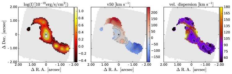
Figure 14: Maps of the observed H$\alpha$ emission obtained from the spatially resolved emission line fit with one Gaussian component. From left to right: integrated observed flux (not corrected for obscuration), 50th percentile velocity ($v50$), velocity dispersion $\sigma$. Contours in the flux map show the [20,40, 60, 80, 90] percentiles, contours in the $v50$ map start at -150 km s^-1and increase every 50 km s^-1, contours in the velocity dispersion map are every 25 km s^-1 at [75, 100, 125, 150, 175] km s^-1.

Fig. 4 shows the maps of the H$\alpha$ emission and kinematics obtained with the best-fit model. For comparison, we also report in the appendix (Fig. 14) the velocity maps obtained with the one-component Gaussian fit, showing no significant differences from those in Fig. 4. The S/N in each line is calculated by taking the ratio of the amplitude of the best-fit model over the noise, estimated by taking the standard deviation of a close spectral region free of line emission.

3.2 R100 data

We fit the R100 data cube to extract the [S iii]$\lambda\lambda 9069,9531$ line fluxes, since this wavelength range is not covered by the R2700 data (see Fig. 2). These fluxes, together with the [S ii]$\lambda\lambda 6717,6731$ fluxes, will be used to estimate the ionisation parameter, as described in Sec. 4.3.5. We use the same methodology as for the fit of the R2700 data cube. In this case, we do not convolve the line width with the line spread function of the NIRSpec PRISM, as we note that in some regions the emission lines are narrower than the values expected according to the spectral resolution curve reported in Jakobsen et al. (2022). This does not affect our results as we are only interested in extracting the line fluxes from the R100 data and not the kinematics.

The continuum is modelled and subtracted before the emission line fit using the same method described above for the R2700 data. Given the low spectral resolution, we just employ one Gaussian to model each line. We model simultaneously the two [S iii] lines, using a single Gaussian component for each line with the same width (in velocity space). We also fit the H$\alpha$, [N ii] and [S ii] complex in a separate fit, forcing the line width to be the same for all the lines. The spectral resolution is too low to resolve the [S ii] doublet, but for the purpose of deriving the ionisation parameter, we only need the sum of the fluxes of the two lines. As specified above, we use the [S iii] fluxes together with the [S ii] fluxes to estimate the ionisation parameter. For this aim, we use [S iii] and [S ii] fluxes derived from the same cube (R100) to avoid potential discrepancies in the flux calibration of the R100 and R2700 observations (e.g. Arribas et al., 2023).

4 Results

4.1 Description of the GS5001 system

The right panel of Figure 1 shows the map of the integrated [O iii] flux of the system (obtained from the emission line fit of the R2700 NIRSpec data cube), together with the HST/ACS F755W image and a NIRCam three-color image (F090W filter in blue, F200W filter in green and F444W filter in red). The ionised gas emission extends over more than 20 kpc and is divided in different structures: a central galaxy, and several components in the south-west and north.

In the south, we identify three sources (s1, s2, s3), two of which are well detected in the HST/ACS image (s1 and s2). These two components were previously identified in the CANDELS catalogue as the source GS4921 (Guo et al., 2013, see Fig. 1). In the north, the [O iii] emission is concentrated in a region to the east of the UV-bright galaxy detected in the HST/ACS image, with CANDELS identifier 4923. This galaxy has a photometric redshift of $z=0.2$ (Pérez-González et al., 2005). Given the lack of emission lines in the NIRSpec data cubes, it is indeed compatible with being a low-redshift foreground galaxy. The [O iii] emission in the north shows three peaks (n1, n2, n3) and a long tail elongated towards the south-east. The [O iii] emission detected in the SINFONI data to the north of GS5001, with a similar redshift and attributed to GS4923 (Ginolfi et al., 2017), is probably coming from this ‘north’ region (see Fig. 1).

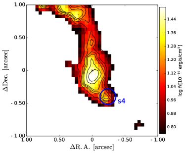
Figure 15: Map of the H$\alpha$ emission in the velocity channels [130, 150] km s^-1with respect to the systemic velocity. The clump on the south-west of the central target (s4) is indicated with a blue circle.

We identify an additional clump (s4) to the south-west of the main source, which is clearly visible in the velocity channels $[130-150]$ km s^-1  (see Fig. 15). Considering that this clump is likely situated between the main galaxy and us (because otherwise, it would be obscured by the main galaxy), and that its emission is redshifted with respect to the main target (by $\sim 70$ km s^-1), we speculate that this clump is moving towards the main galaxy and it is probably in the process of merging. Its relatively low luminosity suggests a minor merger event.

We also detect diffuse ionised gas emission in the regions in between the three components (called ‘main’, ‘south’ and ‘north’ from now on). The peak of the [O iii] (and H$\alpha$) line emission in the main galaxy is shifted to the south by $\sim 0.1"$ (0.7 kpc ) with respect to the peak of the continuum emission in the HST/ACS F775W band (marked with a cross in the figure). This may be due to obscuration (see Sec. 4.3.1).

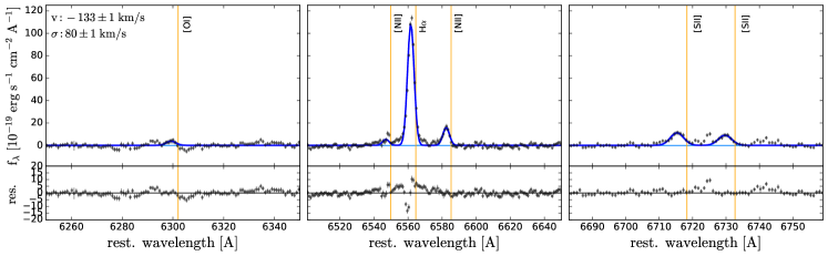
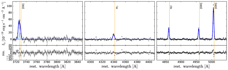
Figure 19: Integrated spectrum of source ‘south’. The total best fit is shown in blue. The uncertainties on the fit are illustrated with grey curves. The vertical lines mark the wavelength positions of the emission lines at the systemic redshift of the main source ($z=3.47046)$. The fitting residuals are shown in the bottom panel.

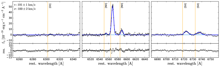
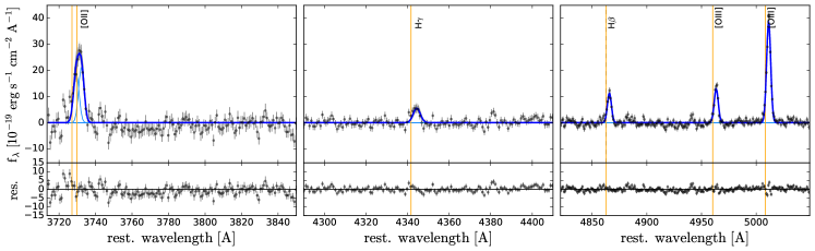
Figure 19: Integrated spectrum of source ‘north’.

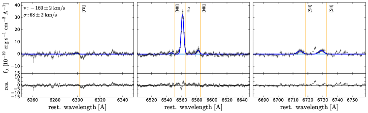
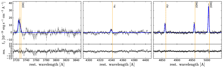
Figure 19: Integrated spectrum of source ‘s1’.

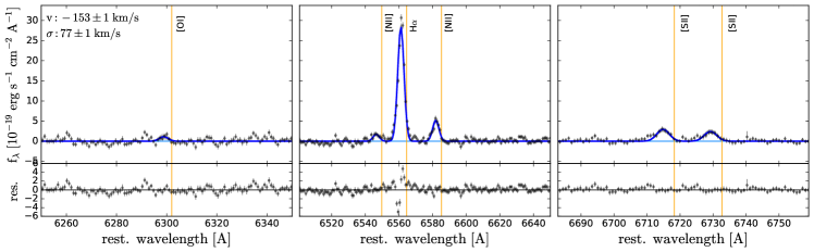
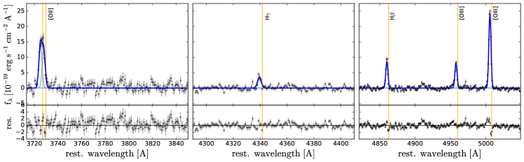
Figure 19: Integrated spectrum of source ‘s2’.

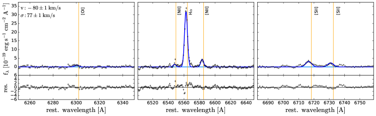
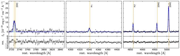
Figure 19: Integrated spectrum of source ‘s3’.

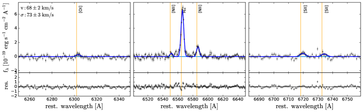
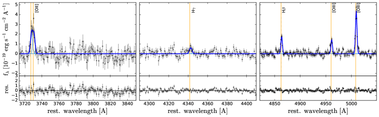
Figure 19: Integrated spectrum of source ‘s4’.

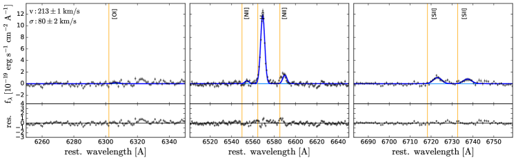
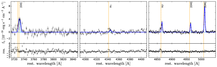
Figure 19: Integrated spectrum of source ‘n1’.

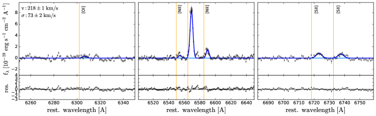
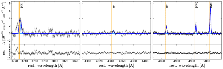
Figure 19: Integrated spectrum of source ‘n2’.

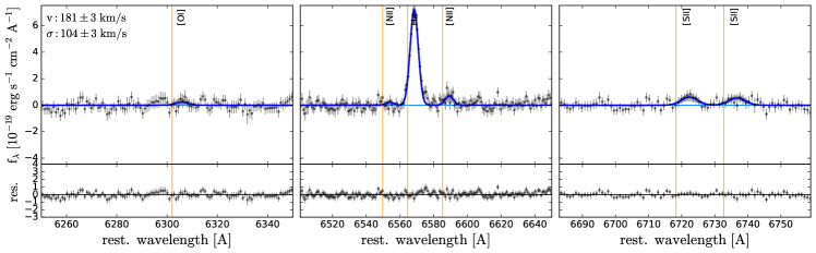
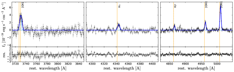
Figure 19: Integrated spectrum of source ‘n3’.

The integrated spectrum of the main galaxy is shown in Fig. 3, and Fig 19 in the appendix shows the integrated spectra of the other components (s1, s2, s3, s4, n1, n2, n3, north). The physical properties of the different components of the system, derived from the modelling of these integrated spectra, are reported in Table 1.

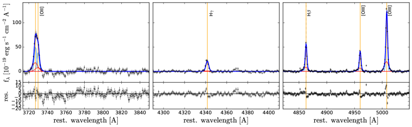
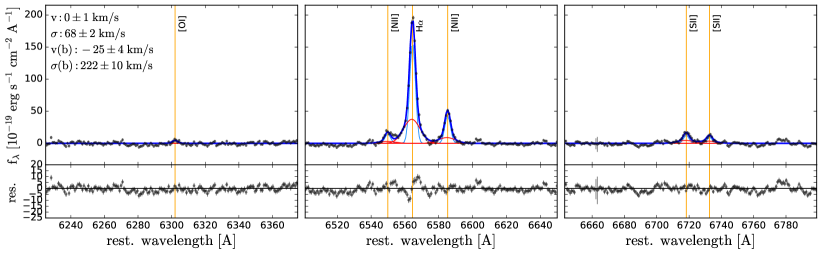
Figure 3: Integrated spectrum of GS5001 (‘main’ source in Fig. 1). Data are shown in black, the total best fit in blue, the narrow and broad components are shown in lightblue and red, respectively. The vertical lines mark the wavelength positions of the emission lines at the systemic redshift of the source ($z=3.47046)$. The fitting residuals are shown in the bottom panel.

Table 1: Physical properties of the different components of the system.

region	$\Delta$RA	$\Delta$Dec	apert.	SFR	AV	12+log(O/H)	log U	ne	$v$	$\sigma$
	[arcsec]	[arcsec]	[arcsec]	[M⊙ yr-1]	[mag.]			[cm-3]	[km s-1]	[km s-1]
(1)	(2)	(3)	(4)	(5)	(6)	(7)	(8)	(9)	(10)	(11)
main∗	0	0	0.25$\times$0.45	180$\pm$1	1.54$\pm$0.07	8.45$\pm$0.04	–2.9$\pm$0.1	540${}^{+120}_{-100}$	–1$\pm$1	93$\pm$1
main narrow				100$\pm$2	1.37$\pm$0.14	8.45$\pm$0.04	-	-	0$\pm$1	68$\pm$2
main broad				-	2.29$\pm$0.53	8.47$\pm$0.07	-	-	–25$\pm$4	222$\pm$10
south	–1.29	–1.00	0.55$\times$0.30	76$\pm$1	1.31$\pm$0.09	8.39$\pm$0.04	–3.1$\pm$0.1	750${}^{+220}_{-180}$	–133$\pm$1	80$\pm$1
north	0.40	0.95	0.45$\times$0.25	106$\pm$1	2.44$\pm$0.16	8.39$\pm$0.06	–2.8$\pm$0.1	150${}^{+130}_{-90}$	191$\pm$1	100$\pm$2
s1	–1.75	–1.05	0.20$\times$0.20	12$\pm$1	0.63$\pm$0.20	8.36$\pm$0.07	–2.7$\pm$0.2	-	–160$\pm$2	68$\pm$2
s2	–1.29	–1.00	0.20$\times$0.20	19$\pm$1	1.34$\pm$0.13	8.41$\pm$0.04	–3.2$\pm$0.1	630${}^{+210}_{-180}$	–153$\pm$1	77$\pm$1
s3	–0.84	–0.80	0.20$\times$0.20	30$\pm$1	1.75$\pm$0.10	8.37$\pm$0.05	–2.7$\pm$0.2	200${}^{+130}_{-100}$	–80$\pm$1	77$\pm$1
s4	–0.30	–0.40	0.12$\times$0.12	6$\pm$1	1.75$\pm$0.25	8.44$\pm$0.07	–3.2$\pm$0.2	-	68$\pm$2	73$\pm$3
n1	0.18	0.92	0.12$\times$0.12	12$\pm$1	1.82$\pm$0.16	8.42$\pm$0.05	–2.9$\pm$0.2	260${}^{+200}_{-150}$	213$\pm$1	80$\pm$2
n2	0.40	1.05	0.12$\times$0.12	13$\pm$1	2.43$\pm$0.22	8.36$\pm$0.07	–3.0$\pm$0.2	510${}^{+320}_{-220}$	218$\pm$1	73$\pm$2
n3	0.75	0.98	0.15$\times$0.15	27$\pm$1	3.20$\pm$0.48	8.34$\pm$0.11	–3.1$\pm$0.1	-	181$\pm$3	104$\pm$3

Table 2: Emission line fluxes of the different components of the system, in units of [$\times 10^{-18}$ erg s^-1 cm^-2].

region	[O ii]$\lambda 3726$	[O ii]$\lambda 3729$	H$\gamma$	H$\beta$	[O iii]$\lambda 5007$	H$\alpha$	[N ii]$\lambda 6584$	[S ii]$\lambda 6716$	[S ii]$\lambda 6731$
main	$180.7\pm 1.9$	$127.3\pm 0.8$	$45.2\pm 0.4$	$106.8\pm 0.4$	$227.6\pm 0.4$	$305.3\pm 0.8$	$78.6\pm 0.5$	$28.1\pm 0.7$	$20.9\pm 0.3$
main narrow	$77.9\pm 1.7$	$60.9\pm 0.9$	$28.4\pm 0.4$	$59.6\pm 0.6$	$125.8\pm 0.6$	$170.3\pm 1.2$	$43.1\pm 0.7$	$14.6\pm 0.6$	$11.0\pm 0.4$
main broad	$316.1\pm 4.0$	$134.0\pm 1.4$	$11.2\pm 0.6$	$89.7\pm 1.1$	$197.5\pm 1.8$	$256.4\pm 4.0$	$63.8\pm 1.7$	$26.7\pm 1.1$	$21.1\pm 0.8$
south	$81.9\pm 1.6$	$60.1\pm 0.7$	$21.3\pm 0.3$	$45.0\pm 0.3$	$125.0\pm 0.4$	$128.6\pm 0.6$	$18.8\pm 0.4$	$13.2\pm 0.7$	$10.7\pm 0.3$
north	$189.8\pm 1.0$	$210.9\pm 0.5$	$42.1\pm 0.3$	$63.2\pm 0.2$	$202.5\pm 0.3$	$180.7\pm 0.4$	$29.2\pm 0.3$	$20.9\pm 0.4$	$15.7\pm 0.2$
s1	$8.6\pm 1.0$	$5.6\pm 0.4$	$2.1\pm 0.2$	$6.9\pm 0.2$	$20.2\pm 0.3$	$19.9\pm 0.4$	$2.1\pm 0.3$	$1.7\pm 0.3$	$1.9\pm 0.2$
s2	$23.3\pm 0.5$	$19.4\pm 0.2$	$5.0\pm 0.1$	$11.5\pm 0.1$	$31.2\pm 0.1$	$32.8\pm 0.2$	$6.0\pm 0.1$	$3.4\pm 0.2$	$2.8\pm 0.1$
s3	$30.9\pm 0.4$	$24.1\pm 0.2$	$9.2\pm 0.1$	$17.9\pm 0.1$	$54.3\pm 0.1$	$51.3\pm 0.1$	$6.9\pm 0.1$	$4.9\pm 0.1$	$3.5\pm 0.1$
s4	$6.1\pm 0.2$	$5.6\pm 0.1$	$1.4\pm 0.1$	$3.5\pm 0.1$	$8.1\pm 0.1$	$9.9\pm 0.1$	$2.2\pm 0.1$	$0.7\pm 0.1$	$0.6\pm 0.1$
n1	$12.1\pm 0.2$	$10.3\pm 0.1$	$2.0\pm 0.1$	$7.2\pm 0.1$	$17.7\pm 0.1$	$20.6\pm 0.1$	$2.6\pm 0.1$	$1.8\pm 0.1$	$1.4\pm 0.1$
n2	$24.5\pm 0.2$	$21.4\pm 0.1$	$4.1\pm 0.1$	$7.5\pm 0.1$	$27.2\pm 0.1$	$21.5\pm 0.1$	$3.8\pm 0.1$	$2.1\pm 0.1$	$1.8\pm 0.1$
n3	$97.6\pm 0.4$	$78.1\pm 0.2$	$31.5\pm 0.1$	$16.0\pm 0.1$	$78.1\pm 0.1$	$45.8\pm 0.1$	$4.3\pm 0.1$	$3.7\pm 0.1$	$3.3\pm 0.1$

Table 3: Fluxes of the different components of the system derived from the R100 data cube, in units of [$\times 10^{-18}$ erg s^-1 cm^-2].

region	[S ii]$\lambda 6716$ + $\lambda 6731$	[S iii]$\lambda 9069$	[S iii]$\lambda 9531$
main	$55.3\pm 6.7$	$17.4\pm 3.3$	$43.0\pm 4.1$
north	$22.9\pm 3.1$	$8.4\pm 1.2$	$21.0\pm 1.4$
s1	$4.0\pm 0.8$	$2.0\pm 0.6$	$3.8\pm 0.8$
s2	$8.1\pm 0.9$	$1.5\pm 0.4$	$4.7\pm 0.6$
s3	$6.5\pm 1.3$	$2.3\pm 0.7$	$7.6\pm 0.8$
s4	$2.6\pm 0.4$	$0.6\pm 0.2$	$1.4\pm 0.2$
n1	$3.0\pm 0.6$	$1.0\pm 0.2$	$2.7\pm 0.3$
n2	$3.8\pm 0.6$	$1.1\pm 0.3$	$2.6\pm 0.3$
n3	$6.7\pm 0.9$	$1.1\pm 0.2$	$4.4\pm 0.3$

4.2 Kinematic properties

4.2.1 Velocity maps

Figure 4 shows the maps of the H$\alpha$ line derived from the fit with one or two Gaussian components. The optimal number of Gaussian components to be used in each spaxel was selected based on a BIC threshold. The maps show the total observed line flux (not corrected for obscuration), the velocity at the peak of the line, and the line width W80 (width encompassing 80% of the line emission, calculated as the difference between the 10th and 90th percentiles velocities). The zero velocity is determined based on the redshift of the central target, derived from the integrated spectrum ($z=3.47046\pm 0.00010$).

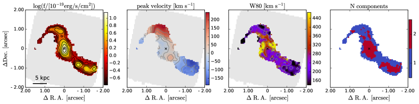
Figure 4: Maps of the observed H$\alpha$ emission obtained from the emission line fit with the best-model (with one or two Gaussian components). The number of components used for the fit in each spaxel is indicated in the right panel. From left to right: integrated observed flux (not corrected for obscuration), velocity at the peak of the emission, line width W80 (width encompassing 80% of the flux), number of Gaussian components used in the fit. Contours in the flux map show the [20, 40, 60, 80, 90] percentiles; contours in the velocity map start at –150 km s^-1and increase every 50 km s^-1; contours in the W80 map are at [200, 300, 400] km s^-1.

The southern clumps s1, s2, and s3 have velocities blue-shifted by $-160,-153,-80$ km s^-1, respectively, with respect to the central galaxy. The northern clumps n1, n2, and n3 instead are redshifted by $213,218,182$ km s^-1, respectively, and the tail shows a velocity gradient going from $\sim 100$ km s^-1 close to the north galaxy to $-100$ km s^-1 towards the SE direction.

In the central galaxy, we see a gradient with the velocity increasing from –30 km s^-1 in the north-east to 50 km s^-1 in the south-west. If we interpret this gradient as rotation, the kinematic major axis is roughly along the NE-SW direction. We note that the direction of this velocity gradient (kinematic major axis) is not aligned with the photometric major axis, which is roughly in the N-S direction (shift of $\sim 40^{\circ}$ between photometric and kinematic major axes), as commonly observed in interacting systems and mergers at low-redshift (e.g. Barrera-Ballesteros et al., 2015; Perna et al., 2022). The peak velocity increases at the location of the clump s4, which indeed has a velocity redshifted by $\sim 140$ km s^-1. If we were to exclude this clump, the velocity gradient could be more aligned with the E-W direction, instead of NE-SW. However, the low S/N prevents us from separating the s4 clump from the rest of the galaxy, so, the direction of the kinematic axis remains uncertain.

We note that the velocities of the companions do not follow the rotation of the central target. The NW part of the central target has blueshifted velocities, while the north companion has redshifted velocities. Similarly, the SE part of the central target shows redshifted velocities while the south companions have bluer velocities.

The W80 map shows values in the range 140-450 km s^-1, with lower values in the companions (140-250 km s^-1, see third panel in Fig. 4). This map shows two regions with enhanced values in the main target (W80 ¿ 400 km s^-1). They lie at the edge of the emission, roughly aligned with the photometric minor axis. These regions could indicate the presence of an outflow. This possibility is discussed in details in the next Sec. 4.2.2. Enhanced line width (W80$>300$ km s^-1) is also seen at the boundary between the central and north galaxies, possibly due to the superposition along the line-of-sight of the emission coming from two or more components with different velocities, or by an enhanced turbulence produced by interactions.

4.2.2 Outflow

The integrated spectrum of the main target (see Fig. 3) shows two kinematic components: a narrow and a broad component clearly detected both in the Balmer lines H$\alpha$ and H$\beta$, and also in [O iii] and [N ii]. We consider the broad component, which has a velocity dispersion of $\sigma\sim 220$ km s^-1, as indicative of an outflow. Additionally, the W80 map shows two regions with large line widths (see Fig. 4), that could be due to the outflow.

We analyse the H$\alpha$ line in order to characterise this broad component, since it is the line with the highest S/N. In Figure 5 we show the H$\alpha$ spectra from the two regions with enhanced velocity dispersion ($\sigma>160$ km s^-1, or W80 $>350$ km s^-1) in the E and W parts of the main galaxy, extracted within circular apertures of radius 0.15$\arcsec$, together with the spectrum of the central region, extracted within an aperture of radius 0.10”. We fit these spectra using a two-component model. In these two regions, the broad component is very prominent compared to the flux of the narrow component, while in the central region the narrow component dominates, giving a much smaller W80 of the total profile ($\sim 250$ km s^-1). The broad components have a velocity dispersion $\sigma\sim 200-300$ km s^-1and the $v05$ and $v95$ of the total profile are $\sim\pm 400$ km s^-1. The broad component in these two external regions has a very small velocity shift with respect to the systemic velocity, making the shape of the total profile fairly symmetric. All these morphological and kinematic characteristics are compatible with a bi-conical outflow. The two regions with high velocity dispersion are in the direction of the photometric minor axis, as expected from star-formation-driven outflows, which typically expand perpendicular to the disk (e.g. Bellocchi et al., 2013). We discuss the properties and possible origin of the outflow in Sec. 5.2.

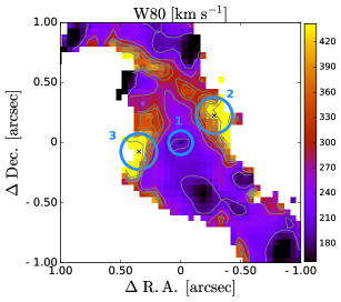
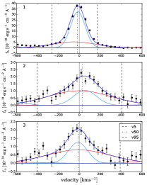
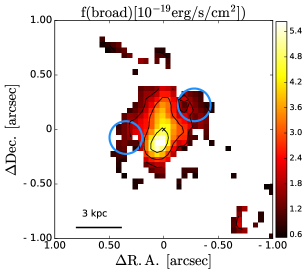
Figure 5: Left panel: Map of the line width (W80) of H$\alpha$ derived from the best-fit model. The three circles indicate the extraction regions of the spectra shown on the middle panel. Middel panel: Comparison of the spectra extracted from the central region (upper row, radius=0.1″), and from the two regions with high velocity dispersion (middle and bottom row, radius=0.15″). The extraction regions are shown in the left panel. Right panel: Map of the H$\alpha$ broad component flux. This map is created by adding the flux of all Gaussian component with $\sigma>140$ km s^-1. This map has not been corrected for obscuration. Lightblue circles mark the positions of the regions 2 and 3.

4.3 Properties of the ISM

4.3.1 Dust attenuation

We measure the dust attenuation in each spaxel using the Balmer decrement H$\alpha$/H$\beta$. We use the results of the fit with only one component across the whole data cube, as we are interested in the obscuration of the dominant gas component (i.e. not the outflow). We assume a theoretical value of H$\alpha$/H$\beta$= 2.86, estimated for Case B recombination assuming a temperature of $10^{4}$ K and an electron density $n_{e}=10^{2}-10^{3}$ cm^-3 (Osterbrock & Ferland, 2006). We adopt the Cardelli et al. (1989) attenuation law. We derive the attenuation for the global emission inferred from the one-component fits, as the S/N of the broad component is not high enough to derive reliable line ratios separately for the broad and narrow components in individual spaxels, nor binning $3\times 3$ adjacent spaxels. We will discuss the attenuation of the outflow component detected in the integrated spectrum in Sec. 5.2.

Figure 6 shows the map of the visual attenuation $A_{V}$. The central galaxy has $A_{V}=0.5-2.7$. The attenuation is enhanced in a region $\sim 0.3-0.5^{\prime\prime}$ to the NW and in a region $\sim 0.2-0.4"$ to the SW from the centre. A region with lower attenuation is found close to the centre and extending towards the SE. This low-attenuation region corresponds to an area with high ionisation parameter (traced by [S iii]/[S ii], see section 4.3.5).

The high attenuation in the region between the main component and the north component corresponds to a dust lane that is visible in the composite NIRCam image shown in Fig. 1. In Figure 6, we show with contours the location where the ratio of the F444W/F090W NIRCam maps is higher, to highlight the region with redder color, that we interpret as a dust lane.

The northern component (particularly the n2 and n3 clumps) and the south clump s3 show the highest attenuation values ($A_{V}>2.4$, see Table 1). These components were not detected in the HST UV map (see Fig. 1): the low UV fluxes could indeed be due to the high attenuation. The clump s1 instead shows the lowest $A_{V}\sim 0.2-0.7$.

In summary, we observe a rather heterogeneous distribution of dust over the system with typical sub-kpc variations of $A_{V}\sim 1$ mag. The least obscured regions ($A_{V}<0.5$ mag.) are found at the south, while those most attenuated ($A_{V}>2$ mag) are in the north component and associated with a dust lane identified by NIRCam broad band imaging (see Fig. 6). We also find a relatively low attenuated region in the main target, to the south-east of the centre, corresponding to an area with high ionisation parameter (see Sec. 4.3.5). We use this $A_{V}$ map to correct for attenuation the fluxes of the measured emission lines.

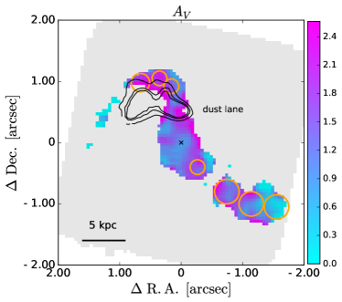
Figure 6: Visual attenuation map inferred from the H$\alpha$/H$\beta$ line ratio, using the Cardelli et al. (1989) reddening law. We show spaxels with S/N(H$\alpha$)$>3$ and S/N(H$\beta$)$>2$. Contours indicates the dust lane identified in the map ratio of the NIRCam F444W/F090W filters. Orange circles indicate the position of the components identified in Fig. 1.

4.3.2 Emission line diagnostics of gas excitation mechanisms

In this subsection, we investigate the source of ionisation in a spatially resolved way. In Figure 7, we present the maps of the line ratios [N ii]/H$\alpha$ and [O iii]/H$\beta$, together with the emission line diagnostic diagram (BPT; Baldwin et al., 1981). We show here all the spaxels with S/N¿3 in the H$\alpha$, H$\beta$, [N ii] and [O iii] lines.

The line ratios in our target are all below the separation line between star formation and AGN found by Kewley et al. (2001) for local sources, thus, they are consistent with ionisation from HII regions. The line ratios are higher than the typical line ratios of star-forming galaxies in the local Universe (see SDSS contours), but they follow quite well the locus of star-forming galaxies at $z=2-3$ from the KBSS-MOSFIRE sample presented by Strom et al. (2017). Recently, some high-redshift AGN discovered by JWST have been reported to be on the same location of the KBSS-MOSFIRE sample (Übler et al., 2023; Maiolino et al., 2023; Scholtz et al., 2023). However, our target is at a lower redshift and more metal rich (see Sec. 4.3.3) than the AGN explored in those JWST studies, thus the BPT classification should still be reliable. The scatter in our points is partly due to uncertainties (the average uncertainties are of the order of 0.1 dex). The south and north companions, shown with light-blue and red dots, respectively, have lower [N ii]/H$\alpha$ and higher [O iii]/H$\beta$ values compared with the main target (orange dots). This is consistent with these targets having lower metallicity (see Sec. 4.3.3).

The north part of the main target shows the highest values of [N ii]/H$\alpha$ and lowest [O iii]/H$\beta$ values. We investigate two possible mechanisms that could explain these line ratios. One possibility is that the [N ii]/H$\alpha$ ratio is enhanced by shocks. If the line ratios are driven by shocks, they are expected to correlate with the kinematics of the gas (e.g Monreal-Ibero et al., 2006; Arribas et al., 2014; Ho et al., 2014; McElroy et al., 2015; Perna et al., 2017, 2020; Mingozzi et al., 2019; Johnston et al., 2023). The velocity dispersion in that region is indeed higher than in the south part of the main target (see W80 map in Fig. 4). In Fig. 8 we show the line ratio [N ii]/H$\alpha$ versus the velocity dispersion. The points in Fig. 8 are color-coded according to a combination of the two quantities on the x and y axes, using the expression from Eq. 1 in D’Agostino et al. (2019).

$$Q=\frac{X-min(X)}{max(X)-min(X)}\times\frac{Y-min(Y)}{max(Y)-min(Y)},$$ (1)

where $X=\log$ [N ii]/H$\alpha$ and $Y$ is the velocity dispersion $\sigma$. The upper panel of Fig. 8 shows the map of the system color-coded by $Q$, illustrating that the highest values of velocity dispersion and [N ii]/H$\alpha$ are found in the northern part of the main galaxy. There is an overall correlation between the two quantities (Spearman’s rank correlation coefficient $r=0.71$, $p$-value $<0.01$). The slope of the correlation is flatter at low values of $\log$ [N ii]/H$\alpha$¡ 0.6, and then it becomes steeper and more scattered at higher [N ii]/H$\alpha$ values. This could indicate that the shocks are affecting the line ratios in regions with high velocity dispersion ($\sigma>100$ km s^-1), while at lower $\sigma$ photo-ionisation is probably the main mechanism driving the changes in the line ratio.

In Fig. 8, we overlaid a set of shock models calculated with the code MAPPING V (Sutherland & Dopita, 2017; Sutherland et al., 2018). We use the 3MdBs database (Alarie & Morisset, 2019) to download the grid of models presented in Allen et al. (2008). We consider models with solar metallicity, magnetic fields values in the range 1-10 $\mu$G, and pre-shock densities in the range of $1-10$ cm^-3 (which correspond to [S ii]-based post-shock electron densities in the range $50-4000$ cm^-3). The models assume shock velocities ¿100 km s^-1. In the velocity range covered by both the observations and the models (100-160 km s^-1), the shock models match the observed [N ii]/H$\alpha$ line ratios.

Another possibility is that the enhanced [N ii]/H$\alpha$ and diminished [O iii]/H$\beta$ line ratios is due to higher metallicity in that region. We will discuss this possibility further in the next section. In summary, the spatially resolved [O iii]/H$\beta$ and [N ii]/H$\alpha$ line ratios are consistent with emission due to star formation, with no sign of AGN ionisation. We find a region with enhanced [N ii]/H$\alpha$ and low [O iii]/H$\beta$, located in the northern part of the main target. This peculiar line ratios could be due to shocks, or to a higher metallicity.

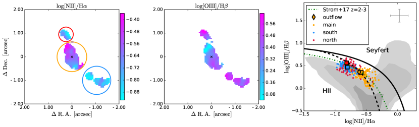
Figure 7: Spatially resolved maps of the emission line ratios [N ii]/H$\alpha$ and [O iii]/H$\beta$. The circles show the color-coding for the spaxels in the BPT diagram in the right panel. Right: Emission line diagnostic diagram for the single spaxels. Spaxels belonging to the north, main, and south regions are indicated in red, orange, and light blue, respectively. A representative (median) errorbar is shown in the top right. The line ratios derived from the integrated spectra of the three regions are shown with squares. The orange diamond shows the line ratios of the outflow, derived from the broad component of the integrated spectrum of the main target. In black are shown the demarcation lines from Kewley et al. (2001) (solid) and Kauffmann et al. (2003) (dashed). The green dashed line show the locus of star-forming galaxies at $z=2-3$ from Strom et al. (2017). The location of galaxies from the SDSS sample (Abazajian et al., 2009) is illustrated with the grey contours showing the 50th, 90th, and 98th percentiles of the sample.

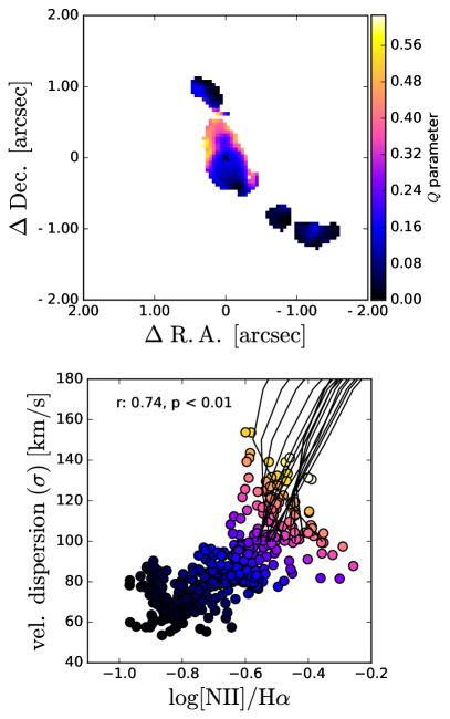
Figure 8: Lower panel: Emission line ratios [N ii]/H$\alpha$  versus the velocity dispersion for individual spaxels. Points are color-coded based on the function $Q$ described in Equation 1, which combines [N ii]/H$\alpha$ and velocity dispersion. Black curves show shock models derived with MAPPINGS V (see text). Upper panel: Map color-coded as in the lower panel, showing the region with high [N ii]/H$\alpha$  and high velocity dispersion.

1

4.3.3 Gas-phase metallicity

In this section, we study the gas-phase metallicity in our system. We calculate the gas-phase metallicity following the prescriptions from Curti et al. (2020b, 2024). We prefer to use these prescriptions even if they are calibrated for local galaxies, because prescriptions for higher redshift galaxies do not cover well the high metallicity regime (12+log(O/H)¿ 8.4, e.g. Sanders et al., 2024). We consider the metallicity indicators based on the line ratios R3=[O iii]$\lambda$5007/H$\beta$, O3O2=[O iii]$\lambda$5007/[O ii]$\lambda$3727,3729, and R23= ([O ii]$\lambda$3727,3729+ [O iii]$\lambda$4959,5007)/H$\beta$. We decide to use this set of line ratios, because they are appropriate for the metallicity regime of our target. We did not include the N2 = [N ii]/H$\alpha$ line ratio because, as we have seen in Sec. 4.3.2, it may be affected by shocks. We fit simultaneously the R3, O3O2 and R23 parameters to reduce the uncertainties, following the procedure described in Curti et al. (2024).

From the integrated spectrum of the main target we measure $\text{12+log(O/H)}=8.45\pm 0.04$. For the stellar mass of GS5001, i.e. $\log(M_{\star}/M_{\odot})=10.0-10.6$ (see Sec. 1), the mass-metallicity relation derived by Sanders et al. (2021) for galaxies at $z=3.3$ predicts a metallicity 12+log(O/H)$=8.42-8.49$, consistent with our measurement. The north and south companions show slightly lower metallicities (12+log(O/H)$\sim 8.34-8.44$) compared to the central target. This is expected considering that the companions have a lower stellar mass than the central galaxy. We do not have estimates of the stellar masses for the individual companions, however, for the south source (which includes s1, s2 and s3) there is an estimate from the literature ($\log(M_{\star}/M_{\odot})=9.7-10.4$, see Sec. 1). If we assume the stellar mass is equally divided between the three sub-components, the mass-metalliticy relation by Sanders et al. (2021) would predict 12+log(O/H)$\sim 8.19-8.39$, in agreement with the measured values.

Figure 9 shows a resolved map of the metallicity in the system. The main galaxy shows a metallicity gradient, with lower metallicity in the south (12+log(O/H)=8.4) and a higher metallicity in the NE region, reaching values of 12+log(O/H)=8.58. The lower metallicity in the south could be due to an inflow of lower metallicity gas. We note that in this position we also identify a small clump (s4) that is merging with the main galaxy. This clump could be part of an inflowing stream of gas, or be a lower metallicity companion. We note that the region with low-metallicity observed in the south part of the main galaxy is more extended than the s4 clump. Similar metallicity gradients have been recently reported in galaxies at $z=3.6-7.9$ (Arribas et al., 2023; Rodríguez Del Pino et al., 2024; Venturi et al., 2024), and were explained by possible accretion of low metallicity gas and merger event with a lower-metallicity satellite.

Another possibility is that the north part has been enriched in metals, due to a past episode of enhanced SF activity in the interacting region between the ‘main’ galaxy and the northern component. We note however that the possible presence of shocks in this region (see Fig. 8) may also increase the line ratios mimicking a further rise in metallicity. Then, the derived high metallicities may be a consequence of both enhanced SF and the presence of shocks.

We note that the interacting region shows also a higher level of obscuration with respect to the rest of the galaxy, and that it may be coincident with a dust lane (see Fig. 6). Previous works have found a correlation between the obscuration in the UV (traced by the UV slope) and the gas-phase metallicity (Heckman et al., 1998; Reddy et al., 2010).

In summary, we find that the main galaxy has an average metallicity of 12+log(O/H)$=8.45$ and the companions have slightly lower metallicities ($8.34-8.44$), consistent with the mass-metallicity relation at $z\sim 3$. The main target shows a metallicity gradient with lower values in the SW region and higher in the NE, the region close to the north target. This metallicity gradient could be explained by an inflow of low-metallicity gas or accretion of a lower metallicity companion from the south, or by an increase in the metallicity in the north due to a past star-formation episode triggered by the interaction with the north component.

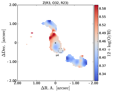
Figure 9: Gas-phase metallicity map calculated using three metallicity calibrations R3, O32, and R23, following the prescriptions from Curti et al. (2020b). The dashed circle shows the position of the clump s4.

4.3.4 Star-formation rates

In Section 4.3.2, we showed that the ionisation in our system is dominated by star formation, thus, we can use the H$\alpha$ luminosity to trace the SFR. We first correct the H$\alpha$ fluxes for obscuration using the Balmer decrement (see Sec. 4.3.1). Then, we convert the H$\alpha$ luminosity into SFR using the relation from Kennicutt & Evans (2012) (see also Murphy et al., 2011; Hao et al., 2011), assuming a Chabrier (2003) IMF.

In Table 1 we report the SFRs derived from the integrated spectra of the different components. For the main target, the SFR derived from the narrow component flux is 100 M_⊙ yr^-1. Considering the star-formation main-sequence definition at $z=3.5$ from Schreiber et al. (2015) and a stellar mass $\log M_{\star}/M_{\odot}=10-10.6$ (see Sec. 1), GS5001 would be 0.1-0.2 dex above the main-sequence. The south clumps have SFRs between 12-30 M_⊙ yr^-1, for a combined SFR of $\sim 76$ M_⊙ yr^-1, while the north component has a total SFR of 106 M_⊙. Thus, the north and south companions have a total SFR comparable to the main target, and the total SFR of the system is $\sim 300$ M_⊙ yr^-1. Previous estimates of the SFR, derived from SED fitting, were in the range 150-240 M_⊙ yr^-1 for the central galaxy and in the range 60-110 M_⊙ yr^-1 for the south component, consistent with our measurements within a factor of two (see Sec. 1).

Figure 10 shows the maps of the SFR surface density ($\Sigma_{SFR}$) derived from H$\alpha$, together with the F090W NIRCam image, tracing the UV flux at $\leavevmode\nobreak\ \sim 2000$ Å  rest-frame. In the F090W image, we can identify three peaks in the central target, aligned in the N-S direction. The region with the highest $\Sigma_{SFR}$ is also aligned in the same direction. Overall, the $\Sigma_{SFR}$ is very high in the central target, where it reaches values of $\sim 10$ M_⊙ yr^-1kpc^-2. Also in the companions the values are relatively high, in the range $0.3-6$ M_⊙ yr^-1kpc^-2.

SFR densities for galaxies at redshift $z>3$ have been reported in the literature, mainly from integrated measurements (e.g. Reddy et al., 2023a, b; Morishita et al., 2024). Thanks to NIRSpec IFS, it is now possible to derive spatially resolved maps. Rodríguez Del Pino et al. (2024) reported similar high values ($\Sigma_{SFR}\sim 8$ M_⊙ yr^-1kpc^-2) in the central region of GS4891, a star-forming galaxy at z=3.7, also part of the GA-NIFS sample. Morishita et al. (2024) finds similarly high values ($\Sigma_{SFR}>10$ M_⊙ yr^-1kpc^-2) in a sample of compact sources at $z>5$.

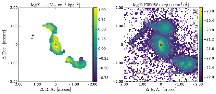
Figure 10: Left: Map of the SFR surface density, inferred from the dust-corrected H$\alpha$ luminosity. Right: flux in the NIRCam filter F090W.

4.3.5 Ionisation parameter

We calculate the ionisation parameter U, i.e. the ratio of (hydrogen-)ionising photons over the gas density, using the prescriptions from Diaz et al. (1991); Diaz (1999). We consider the calibrations involving the flux line ratio S2S3=([S ii]$\lambda$6717+[S ii]$\lambda$6731)/([S iii]$\lambda$9069+[S iii]$\lambda$9531), measured from the R100 data cube. The S2S3 line ratio is less dependent on metallicity than O3O2, thus it is considered to be a more accurate estimator of the ionisation parameter (Mathis, 1982; Dopita & Evans, 1986; Kewley & Dopita, 2002; Kewley et al., 2019; Mingozzi et al., 2020).

The values of the ionisation parameter derived from the integrated spectra of the different components of the system are reported in Table 1. The values of the ionisation parameter span a range from log U = [-3.1, -2.7]. These values are within the range measured by Reddy et al. (2023a) using the O3O2 ratio in a sample of galaxies at $z=1.9-3.7$ (log U = [-3.25, -2.05]).

Figure 11 shows the map of the ionisation parameter obtained using the S2S3 calibrations. We show only spaxels with S/N¿3 in the sum of the [S iii] and [S ii] lines (i.e. S/N([S iii]$\lambda$9069)+S/N([S iii]$\lambda 9531)>3$ and S/N([S ii]$\lambda$6717)+S/N([S ii]$\lambda 6731)>3$) and with S/N(H$\beta$$)>2$, to ensure that we can correct the fluxes for obscuration using the Balmer decrement. The values of the ionisation parameter span a range from log U = -3.8 to -2.3. In the main target, the ionisation parameter is enhanced (by $\sim 0.4$ dex) with respect to the rest of the galaxy in a region south of the continuum peak pointing toward the south-east. We note that this region has lower obscuration ($A_{V}$) than the rest of the main galaxy (see Fig. 6). The clump s3 also shows a similar enhancement of the ionisation parameter. We note that these regions corresponds to the regions with brighter H$\alpha$ flux, and therefore higher SFR (see Fig. 10). The north companion and the clumps s1 and s2 have low ionisation parameter (log U $<-3$) similar to the values in the north part of the main target.

We calculated the ionisation parameter maps also using the O3O2, S2H$\beta$ and O2H$\beta$ calibrations from Díaz et al. (2000). These maps show similar spatial variations, even though the normalisation is different.

In our target, we observe that the regions with high ionisation parameter (region south of the continuum peak, and clump s3) correspond to regions with elevated SFR surface density (see Fig. 10). A correlation between ionisation parameter and SFR surface density has been observed in previous spatially resolved studies of nearby galaxies (Dopita et al., 2014; Kaplan et al., 2016), but also within a galaxy sample at $z=1.9-3.7$ (Reddy et al., 2023a). This correlation suggests that SFR plays an important role in regulating the ionisation parameter (Reddy et al., 2023a).

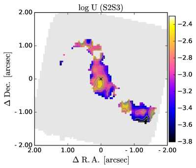
Figure 11: Maps of the ionisation parameter derived from the S2S3 line ratio. We show only spaxels with S/N¿2 in H$\beta$, and S/N¿3 in the the sum of the [S iii] and [S ii] lines.

4.3.6 Electron density

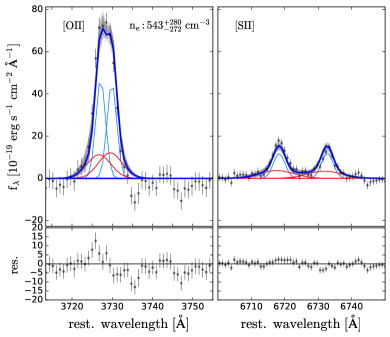
Figure 18: Simultaneous spectral fit of the [O ii]$\lambda\lambda 3726,29$ and [S ii]$\lambda\lambda 6716,31$ doublets to derive the electron density from the integrated spectrum of the main target using two components (broad and narrow). The blue curve shows the total best-fit model, the light-blue curves show the best-fit Gaussians for the individual emission lines, and the gray curves the uncertainties of the MCMC fit. The bottom panels show the residuals.

The electron density can be derived using the ratios of the [S ii]$\lambda\lambda$6716,31 or the [O ii]$\lambda\lambda$3726,29 doublets (Osterbrock & Ferland, 2006). In our case, the S/N is not enough to study these line ratios spaxel-by-spaxel, thus, we focus on the integrated spectra. We note that the two [O ii] lines are not fully spectroscopically resolved in our data. On the other hand, the [S ii] lines are well resolved, but have lower S/N. In order to better constrain the electron density, we fit simultaneously the [S ii] and [O ii] lines, forcing the line ratios to agree on the same $n_{e}$ parameter, following the same approach used by Rodríguez Del Pino et al. (2024). We use the formulas presented in Sanders et al. (2016) that relate the [S ii] and [O ii] line ratios to the electron density. We do not attempt to model the emission lines with two components (broad and narrow), because even in the integrated spectrum of the main galaxy the S/N of the broad component is not high enough to derive meaningful constraints on the electron density (see Fig. 18 in the appendix). The results of the fit of the [O ii] and [S ii] doublets of the main target are shown in Fig. 12.

For the main target, we find $n_{e}=540_{-100}^{+120}$ cm^-3. The independent modelling of the [S ii] line ratio would give $n_{e}$([S ii])$=73_{-50}^{+70}$ cm^-3, while the [O ii] line ratio gives $n_{e}$([O ii])$=1480_{-320}^{+400}$ cm^-3. These estimates have large uncertainties due to the issues mentioned above. We note that the electron densities derived from [O ii] are systematically higher than the ones derived from [S ii] for all the sources in our system. Kewley et al. (2019) highlight that the [S ii] and [O ii] lines are produced in different regions of ionised nebulae: the [S ii] lines are produced in the extended partially ionised region of the nebula, while the [O ii] lines are produced closer to the ionising source. If the density is higher close to the ionising source than further out, this could explain the different $n_{e}$ estimates from [S ii] and [O ii].

We note that the fit of the main galaxy shows significant residuals ($>3\sigma$) on the blue side of the [O ii] doublet (see left panel of Fig. 12). This is probably due to the outflow component that we are not considering in the fit. An attempt to fit simultaneously the [S ii] and [O ii] lines with two components (narrow+broad) gives similar results for the electron density of the narrow component ($n_{e}=540_{-280}^{+270}$ cm^-3), while the electron density of the broad component is unconstrained ($n_{e}=340_{-280}^{+1400}$ cm^-3, see Fig. 18).

For the companions, we find electron densities in the range 200-600 cm^-3 from the simultaneous fit of [O ii] and [S ii]. The values of the electron densities are reported in Table 1.

Our results are consistent with the electron densities of star-forming galaxies at redshift $z\sim 1-2.5$ from the literature (e.g. Masters et al., 2014; Steidel et al., 2014; Shimakawa et al., 2015; Sanders et al., 2016; Kaasinen et al., 2017; Kashino et al., 2017). Recently, Rodríguez Del Pino et al. (2024) measured an electron density of $n_{e}=776\pm 307$ cm^-3 in a star-forming galaxy at a similar redshift $z=3.7$ (GS4891), using NIRSpec data, in agreement with our measurement.

Reddy et al. (2023b) study a sample of $\sim 50$ galaxies at $z=2.7-6.3$, and report average electron densities of $\sim 100-500$ cm^-3. Interestingly, they find higher electron densities ($n_{e}\sim 500$ cm^-3) in galaxies with higher SFR surface density ($\Sigma_{SFR}>1$ M_⊙ yr^-1kpc^-2, see also Reddy et al., 2023a), similar to the $\Sigma_{SFR}$ values observed in GS5001 (see Fig. 10). Recently, Isobe et al. (2023) measure $n_{e}\gtrsim 300$ cm^-3 in a sample of 14 galaxies at $z=4-9$. They find that the $n_{e}$ are higher than those of lower-redshift galaxies with similar values of stellar mass, SFR or specific SFR. GS5001 has a SFR comparable to that of local ULIRGs (SFR ¿ 150 M_⊙ yr^-1), which have an average electron density $\sim 300$ cm^-3 (Arribas et al., 2014), a bit lower than our measurement. This suggests that, apart from an increase in SFR with redshift, the gas conditions at high redshift also lead to higher electron densities (but see also Kaasinen et al. 2017).

In summary, we take advantage of the large wavelength range covered by NIRSpec to measured the electron densities by modelling simultaneously the [S ii] and [O ii] doublets. We measure an electron density of $540^{+120}_{-100}$ cm^-3 in the main targets, and $n_{e}=200-600$ cm^-3 in the companions. We note that using only the [S ii] or [O ii] lines would provide different results, with larger uncertainties.

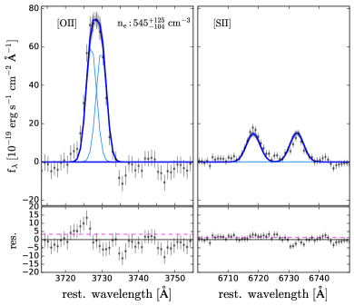
Figure 12: Simultaneous spectral fit of the [O ii]$\lambda\lambda 3726,29$ and [S ii]$\lambda\lambda 6716,31$ doublets to derive the electron density from the integrated spectrum of the main target. The blue curve shows the total best-fit model, the light-blue curves show the best-fit Gaussians for the individual emission lines, and the gray curves the uncertainties of the MCMC fit. The bottom panels show the residuals, the magenta dashed-line indicates the average 1$\sigma$ noise level.

5 Discussion

5.1 Dynamical and physical status of the system: a pre-coalescence merger

Our NIRSpec observations confirm the interesting nature of this system and allow the spatially resolved study of the central galaxy and its close companions ($<15$ kpc). We observe signs of interactions between the northern companion and the central galaxy: in the this region, the ionised gas is more turbulent and the ISM shows peculiar properties (higher [N ii]/H$\alpha$, higher metallicity, and higher obscuration than elsewhere). Additionally, the north component has a tidal tail extending for 10 kpc, which can be interpreted as a sign of interactions. Moreover, we identify one clump (s4) which is probably in the process of merging with the main galaxy. Given the low relative velocities of the companions ($<200$ km s^-1) and projected distance ($<10$ kpc), we can expect that they will coalesce with the central galaxy in the future.

The north and south companions could be part of a large scale gas filament that is feeding the central galaxy. Ginolfi et al. (2017) identify several CO emitters oriented along the NE-SW within a radius of $\sim 250$ kpc. They interpret them as tracers of a cold gas stream feeding the central galaxy. The north and south components, which are broadly oriented along the same direction (see Fig. 13), could have formed in this gas filament and be in the process of moving toward the central galaxy and merging with it, as also suggested by the presence of peculiar ISM properties in the region between the main and north component, and the extended tidal tail towards north-east. Hence, this system may be comparable to the Spiderweb Galaxy at $z\sim 2.2$, where a cloud of molecular gas extending for tens of kpc seems to be feeding the innermost (merging) galaxies in the proto-cluster (Emonts et al., 2016).

Recently, Jin et al. (2023) identified an overdensity consisting of a group of six galaxies within a FoV of $10\times 20$ kpc² at redshift $z\sim 5.2$, CGG-z5, using NIRCam observations. Five companions with $\log(M_{\star}/M_{\odot})\sim 8.4-9.2$ are aligned along two directions around a central more massive galaxy ($\log(M_{\star}/M_{\odot})\sim 9.8$). The geometry look remarkably similar to our system. Jin et al. (2023) look for similar compact structures in the EAGLE cosmological simulations (Crain et al., 2015; Schaye et al., 2015), and follow their evolution with cosmic time. They find that the identified structures will merge into a single galaxy by $z\sim 3$. Therefore, GS5001 could be a similar system, in which all the currently identified structures will merge at a later cosmic epoch.

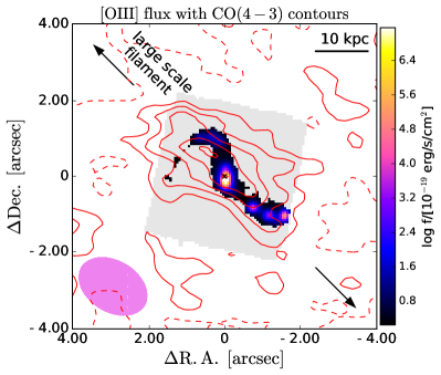
Figure 13: Map of the [O iii] integrated flux with overlaid contours of the CO(4-3) emission from ALMA. Solid contours are at levels $[1,2,3,4,5]$ $\times$ rms, and dashed contours show the $-1\times$ rms level. The magenta oval shows the $1.9^{\prime\prime}\times 1.3^{\prime\prime}$ ALMA beam. Arrows indicate the direction (NW-SE) of the large scale filament traced by CO emitters discovered by Ginolfi et al. (2017).

5.2 The kpc-scale outflow in GS5001: properties, origin and effects

In this section, we describe the properties of gas in the ionised outflow, and we estimate the outflow energetics. As the limited signal-to-noise prevents us from studying the physical properties of the outflow spaxel-by-spaxel, we consider the integrated spectrum of the main target, and use the two-component fit to separate the flux due to the outflow (see Fig. 3).

5.2.1 Outflow properties

The spatially integrated properties of the broad outflow component are reported in Table 1. The dust attenuation measured in the broad component, tracing the outflow, is higher ($A_{V}=2.3\pm 0.5$) compared to the rest of the galaxy ($A_{V}=1.4\pm 0.1$). Higher dust attenuation in the outflows than in the galaxy disk has been observed in several studies at lower redshift (e.g., Holt et al., 2011; Villar Martín et al., 2014; Perna et al., 2015, 2019).

In GS5001 the metallicity of the outflow ($12+\log\text{(O/H)}=8.47\pm 0.07$) is similar to the one derived from the narrow component ($12+\log\text{(O/H)}=8.45\pm 0.04$). The line ratios [N ii]/H$\alpha$ and [O iii]/H$\beta$ in the broad component are also very similar to the ones observed in the narrow component ($\log$ [N ii]/H$\alpha$$=-0.61\pm 0.07$, $\log$ [O iii]/H$\beta$$=0.36\pm 0.07$), thus, the ionisation source of the outflow is compatible with star formation (see Sec. 4.3.2).

We provide here an estimate of the outflow mass and mass outflow rate. We estimate a (projected) outflow radius of 0.4” (3 kpc), corresponding to the distance from the center to the regions with high velocity dispersion (regions 2 and 3 in Fig. 5). To estimate the maximum outflow velocity, we use the average of the absolute values of $v05$ and $v95$ (5th and 95th percentiles) velocities estimated from the integrated spectra of the high-velocity dispersion regions (see Fig. 5), following Cresci et al. (2015); Harrison et al. (2016). As the profiles are symmetric and roughly centred around the zero velocity, $v05$ and $v95$ have a similar value of $v_{max}=400$ km s^-1. Another common definition of the outflow velocity, $v_{\mathrm{out}}=v_{broad}+2\sigma_{broad}$ (e.g. Fiore et al., 2017), would give $v_{\mathrm{out}}=470$ km s^-1 using the velocity parameters derived from the broad component of the integrated spectrum of ‘main’ galaxy, slightly higher than the value estimated from $v05$ and $v95$. We cannot estimate the electron density in the outflow component as the broad component of [S ii] and [O ii] are too faint, so we use the electron density estimated for the total line profile ($n_{e}=540\pm 110$ cm^-3, see Sec. 4.3.6). We calculate the outflow mass following Cresci et al. (2017): $M_{\mathrm{out}}=3.2\cdot 10^{5}\cdot(L_{\mathrm{broad}}(\mathrm{H}\alpha)/10^{40}\text{ erg/s})\cdot(100\text{ cm}^{-3}/n_{e})\text{ M}_{\odot}=(1.7\pm 0.4)\times 10^{8}$ M_⊙. The corresponding mass outflow rate is $\dot{M}_{\mathrm{out}}=M_{\mathrm{out}}\cdot v_{\mathrm{out}}/R_{\mathrm{out}}=23\pm 5$ M_⊙ yr^-1.

We estimate the escape velocity following Arribas et al. (2014). We assume the dynamical mass is twice the stellar mass (Erb et al., 2006), i.e. $M_{dyn}=2-8\times 10^{10}$ M_⊙. We calculate the escape velocity at a radius of 3 kpc (size of the outflow), assuming a truncation radius of 30 kpc. We obtain escape velocities in the range $\sim 330-660$ km s^-1. On the basis of this calculation, we estimate that less than 15% of the outflowing gas has velocities large enough to escape from the galaxy potential well.

5.2.2 Origin of the outflow

As shown in Section 4.2.2, the outflow reaches maximum projected velocities (as traced by $v05$ and $v95$) of $\sim\pm 400$ km s^-1. These velocities are comparable to the velocities measured in ionised outflows driven by star formation (e.g. Arribas et al., 2014; Förster Schreiber et al., 2019; Swinbank et al., 2019). The SFR surface density, estimated from the H$\alpha$ flux, in the central region of GS5001 reaches 10 M_⊙ yr^-1 kpc^-2 (see Fig. 10). This high $\Sigma_{SFR}$ can explain the observed outflow, since it is known that the prevalence of outflows in star-forming galaxies increases with $\Sigma_{SFR}$ (Förster Schreiber et al., 2019). Additionally, the global geometry with the outflow direction roughly aligned with the minor axis is what is expected for a SF-driven outflow.

The mass loading factor, assuming the SFR from the narrow H$\alpha$ component SFR$\sim 100$ M_⊙ yr^-1, is $\eta=\dot{M}_{out}/\text{SFR}=0.23$. The moderate mass loading factor (¡ 1) means that the outflow is not having a significant impact on the total star formation of GS5001. We note however that we are only tracing the ionised outflow, while the molecular and atomic phases of the outflow could also contribute significantly to the total mass outflow rate (e.g. Fiore et al., 2017; Herrera-Camus et al., 2019; Ginolfi et al., 2020; Fluetsch et al., 2021; Belli et al., 2023; D’Eugenio et al., 2023).

The mass loading factor in GS5001 is in agreement with other studies of outflows in star-forming galaxies at lower redshift ($z=0.5-3$). For instance, Förster Schreiber et al. (2019) find average $\eta=0.1-0.25$ in a sample at $z=0.6-2.7$, while Swinbank et al. (2019) report $\eta=0.2-0.4$ in star-forming galaxies at $z\sim 1$. Rodríguez Del Pino et al. (2024) detected a resolved ionised outflow in the star-forming galaxy GS4891 at $z=3.7$, which has a SFR of $\sim 45$  M_⊙ yr^-1. This outflow has a similar outflow velocity of 400 km s^-1, but lower mass outflow rate $\dot{M}_{\mathrm{out}}=2$ M_⊙ yr^-1 and $\eta=0.02$ compared to GS5001, which could be related to the lower SFR of GS4891 compared to GS5001.

5.3 AGN in GS5001?

As discussed in the Introduction, from previous observations it is not clear whether an AGN in present in GS5001. We do not find evidence of AGN activity in the NIRSpec data of GS5001. The emission line diagnostic diagram (BPT, see Fig. 7) shows line ratios similar to other star-forming galaxies at the same redshift, with no spaxels above the AGN separation line. We note that the line ratios for GS5001 do not fall in the region of the BPT diagram where low-metallicity AGN and star-forming galaxies tend to overlap at high redshifts (Maiolino et al., 2023; Scholtz et al., 2023). Our target is at lower redshift and have higher metallicity than the AGN presented in those works, therefore, the classical BPT diagram can still be effectively used to distinguish between AGN and star-forming galaxies.

GS5001 has been detected in the X-ray, with an X-ray luminosity of $L_{0.5-7keV}=(9.5\pm 2.8)\times 10^{42}$ erg s^-1 (Fiore et al., 2012; Luo et al., 2017). In the Chandra Deep Field-South 7Ms catalog (Luo et al., 2017), it has been classified as an AGN, based on an intrinsic X-ray luminosity $L_{0.5-7keV}>3\times 10^{42}$ erg/s. However, for this target no additional criteria could be applied. Therefore, Luo et al. (2017) caution that X-ray emission in this sources may come from intense star formation. A SFR$\sim 520\pm 180$ M_⊙ yr^-1 would be required to explain the observed X-ray luminosity of this target by assuming the Ranalli et al. (2003) relation adapted for a Chabrier (2003) IMF (Kennicutt & Evans, 2012). Thus, the majority of this X-ray luminosity could be explained by the observed SFR of this system (total SFR of the main, south and north components: $\sim 300$ M_⊙ yr^-1). Lyu et al. (2022) classify this galaxy as an AGN based on the X-ray-to-radio luminosity ratio $L_{\textrm{X-ray}}\text{ [erg s${}^{-1}$]}/L_{\textrm{3\,GHz}}\text{ [W Hz${}^{-1}$]}>8\times 10^{18}$. However, we note that GS5001 is only $\sim 0.25$ dex above this threshold and that the X-ray luminosity has been inferred from an extremely small number of counts.

A recent SED analysis including JWST/NIRcam and MIRI photometry up to restframe wavelengths $<6$ $\mu$m classify this galaxy as an AGN, because the AGN template dominates in the range $3-6$ $\mu$m (Lyu et al., 2024). However, given the limited coverage in the infra-red, a fit with a galaxy dust template and a weaker AGN component would still be acceptable. From an SED fitting analysis with the Code Investigating GALaxy Emission (CIGALE; Burgarella et al., 2005; Noll et al., 2009; Boquien et al., 2019) from the UV to the FIR , we find that a strong AGN component in the MIR is not required to produce a good fit (C. Circosta et al., in prep.). In summary, we do not find evidence for an AGN in GS5001, even though we cannot rule out that a weak and possibly obscured AGN is present.

6 Summary and conclusions

In this work, we present JWST/NIRSpec IFS observations of the galaxy GS5001 and its companions at redshift $z=3.47$ within a FoV of $4"\times 4"$ ($30\times 30$ kpc²). We analyse the properties of the emission lines using the high-resolution (R2700) data, complemented by the low-resolution (R100) data, that allow us to cover the optical emission lines from [O ii]$\lambda\lambda 3726,29$ to [S iii]$\lambda 9531$. We fit the data cube to derive the maps of the emission line fluxes as well as kinematic maps of the ionised gas.

The main results of this study are:

• We identify several companions close to GS5001 (main target). In particular, we identify three components in the south (s1, s2, s3), and a companion in the north, with three sub-structures (n1, n2, n3), showing also an extended tail. The south companions show velocities blue-shifted by [-160, -153, -80] km s^-1 with respect to the main target, while the north companion is redshifted by $190$ km s^-1 (see Sec. 4.2).

• The spatially resolved emission line ratios are in the star-forming region of the BPT diagram, with no sign of AGN excitation (see Sec. 4.3.2).

• We estimate the gas-phase metallicity using the R3, R23, and O32 line ratios. We find that the main galaxy has a metallicity of 12+log(O/H)$=8.45\pm 0.04$, and the companions show slightly lower metallicities 12+log(O/H)$=8.32-8.42$, consistent with the mass-metallicity relation at $z\sim 3$. The main galaxy shows higher metallicity in the north-east region, and lower in the south-east (see Sec. 4.3.3).

• From the dust-corrected H$\alpha$ luminosity, we infer a total SFR of 100 M_⊙ yr^-1in the main target. The south companions have a combined SFR of $76\pm 2$ M_⊙ yr^-1 and the north companion a SFR of $106\pm 1$ M_⊙ yr^-1. The SFR surface density reaches values of $\Sigma_{SFR}=10$ M_⊙ yr^-1kpc^-2 in the central region of the main galaxy (see Sec. 4.3.4).

• We find that the region between the north companion and the main target have high [N ii]/H$\alpha$ and low [O iii]/H$\beta$ line ratios, compared with the rest of the main galaxy. These line ratios could be due to the higher metallicity or to shocks. The gas in this region also shows enhanced velocity dispersion, probably due to the interaction between the main and north components (see Sec. 4.3.2).

• We identify an outflow traced by a broad symmetric component clearly visible in H$\alpha$ and [O iii] (with velocity dispersion $\sim 220$ km s^-1, or FWHM of $\sim 520$ km s^-1). The outflow has maximum velocity of $\sim 400$ km s^-1, outflow mass of $(1.7\pm 0.4)\times 10^{8}$ M_⊙, mass outflow rate $23\pm 5$ M_⊙ yr^-1, and a mass loading factor of 0.23 (see Sec. 5.2). This indicates that probably the outflow is not going to impact significantly the star formation in the host galaxy. We note however that we are not tracing the neutral and molecular phases of the outflow.

JWST NIRSpec IFS data allowed us to obtain unprecedented insights into the interplay between star formation, galactic outflows and interactions in the core of a $z\sim 3.5$ candidate protocluster. This valuable information could be used to inform hydrodynamical simulations and therefore follow the evolutionary path of GS5001 and other similar systems, like the Spiderweb Galaxy (Emonts et al., 2016) and CGG-z5 (Jin et al., 2023).

Appendix A H$\alpha$ maps from the one-component Gaussian fit

Appendix B Map of the $\alpha$ emission of clump s4

Appendix C Two component fit: kinematic maps of the broad component of H$\alpha$

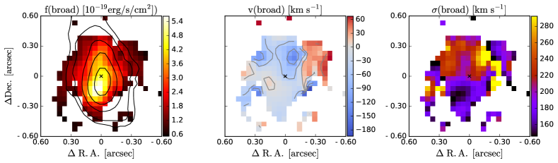
Figure 16: Maps of the broad emission of H$\alpha$, including all Gaussian components with $\sigma>140$ km s^-1. From left to right: observed flux (not corrected for attenuation), velocity, and velocity dispersion. Only spaxels with S/N¿ 3 are shown.

Appendix D Fit of [S ii] and [O ii] for deriving the electron densities

In this section, we show the fit of [S ii] and [O ii] for the four regions in which we could estimate the electron density: s2, s3, n1, n2, and north.

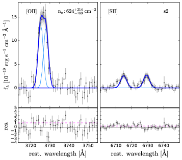
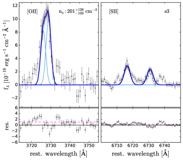
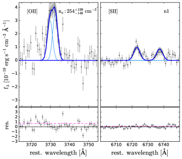
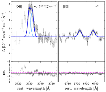
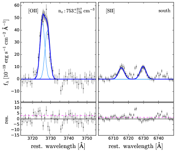
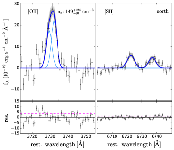
Figure 17: Simultaneous spectral fit of the [O ii]$\lambda\lambda 3726,29$ and [S ii]$\lambda\lambda 6716,31$ doublets to derive the electron density from the integrated spectrum of the targets s2, s3 (upper raw), n1, n2 (middle raw), south and north (lower raw). The blue curve shows the total best-fit model, the light-blue curves show the best-fit Gaussians for the individual emission lines and the gray curves show the uncertainties of the MCMC fit. The bottom panels show the residuals, the dashed line shows the one-sigma error level.

We also show the fit fit of [S ii] and [O ii] lines of the main target using two components (narrow+broad). The electron density derived for the narrow component is similar to the value inferred from the one-component fit but with larger uncertainties ($n_{e}=540_{-280}^{+270}$ cm^-3). The electron density of the broad component is unconstrained ($n_{e}=340_{-280}^{+1400}$ cm^-3).

Appendix E Integrated spectra