Online Identification of Time-Varying Systems Using Excitation Sets and Change Point Detection

Abstract

In this work, we first show that the problem of parameter identification is often ill-conditioned and lacks the persistence of excitation required for the convergence of online learning schemes. To tackle these challenges, we introduce the notion of optimal and greedy excitation sets which contain data points with sufficient richness to aid in the identification task. We then present the greedy excitation set-based recursive least squares algorithm to alleviate the problem of the lack of persistent excitation, and prove that the iterates generated by the proposed algorithm minimize an auxiliary weighted least squares cost function. When data points are generated from time-varying parameters, online estimators tend to underfit the true parameter trajectory, and their predictability deteriorates. To tackle this problem, we propose a memory resetting scheme leveraging change point detection techniques. Finally, we illustrate the performance of the proposed algorithms via several numerical case studies to learn the (time-varying) parameters of networked epidemic dynamics, and compare it with results obtained using conventional approaches.

I Introduction

Accurately predicting unseen events is the hallmark of a successful scientific theory. This predictive capability is essential in transforming theoretical knowledge into tangible benefits, offering understanding and control over complex systems. In particular, the online estimation of system parameters of time-series events holds immense value, as it enables precise anticipation and management of dynamic processes over time. By continuously updating and refining predictions based on incoming data, practitioners can better navigate uncertainties, optimize performance, and mitigate risks [1]. The problem of online system identification has been investigated through adaptive identification methods. Traditional techniques for addressing adaptive identification problems often involve gradient descent and recursive least squares filtering [2]. However, two problems often plague the performance of online parameter estimation: first, the lack of excitation and identifiability of the target system, and second, time-varying system parameters.

Persistent excitation is regarded as the consistent information richness of the unconstrained input signals [3]. It is natural to expect that the persistent excitation condition is sufficient for an adaptive estimation process to converge and track the system parameters. However, this condition is often excessively restrictive [4, 5]. A related challenge in online system identification is the identifiability of unknown parameters. Though the structural identifiability of a model, referring to the theoretical capability to uniquely estimate model parameters from noise-free data, can be analytically verified in various ways for both linear and nonlinear systems [6, 3], a more crucial requirement is practical identifiability [7]. Practical identifiability is the ability to reliably estimate model parameters from real, noisy data, and its absence makes parameter estimation a challenging task, even if it is theoretically feasible.

Contemporary approaches for overcoming the challenges of the lack of persistent excitation and practical identifiability include indirect adaptive control strategies [8] and robust adaptive control methods [9]. Efforts to mitigate the lack of uniform persistent excitation have also explored relaxing this stringent requirement, introducing concepts like initial excitation [10, 11]. Additionally, techniques that incorporate second-order information into each parameter estimation step, such as recursive least squares (RLS) methods [12, 13, 14], have been developed. In this work, we propose a novel algorithm that combines the well-known RLS algorithm with the novel concept of an excitation set that is used to construct the main regressor. We explain the intuition behind this idea, and show that the estimates obtained by the proposed algorithm minimize an auxiliary cost function that weighs exciting data points with unity weight and disregards regressors that are not sufficiently exciting.

Besides, we often encounter systems with time-varying parameters in practice. Previous research has addressed offline system identification problems with piece-wise constant time-varying parameters [15]. Online parameter estimation, however, remains challenging. Some solutions have been proposed through detecting non-stationary statistical properties in the prediction error of recursive least squares [16]. In this work, we combine the exponentially weighted average model [17] and the likelihood ratio test [18] to detect abrupt changes in system parameters through prediction error. Furthermore, we propose a method to incorporate this change point detection and memory resetting algorithm into a broad class of online estimation methods.

Lastly, recognizing the well-documented challenge of practical identifiability in epidemic models as highlighted in recent studies [6, 19], we compare our results with existing approaches. We demonstrate the effectiveness of our algorithm for online parameter identification in time-varying epidemic models [20, 21] with noise. Specifically, we consider the susceptible-infected-susceptible (SIS) and networked susceptible-infected-recovered (SIR) models with time-varying parameters to illustrate the performance of our proposed algorithms.

This paper builds upon our previous work in [22], enhancing it with additional analysis, algorithms, and simulations to address the online estimation challenges present in a broad class of time-varying nonlinear systems beyond single-node SIS systems. We organize the content as follows: in Section II, we present the problem formulation and some necessary definitions for the rest of the paper. In Section II-C, we give a sufficient condition for the lack of persistent excitation In Section III-A, we present the definition of an excitation set and greedy excitation set, which are used to develop the greedily weighted recursive least squares algorithm. In Section III-B, we present the greedily weighted recursive least squares algorithm as a way to overcome the lack of persistent excitation and practical identifiability. In Section IV, we present a way to facilitate tracking of time-varying parameters through memory resetting upon detection of abrupt changes. In Section V, we demonstrate the performance of the proposed algorithms on networked SIS/SIR models.

I-A Notations

We denote a matrix $X$ to be positive and negative semi-definite by $X\succeq 0$ and $X\preceq 0$, respectively. The condition number of a matrix $X$, defined as the ratio of the largest singular value of $X$ to the smallest singular value of $X$, is denoted by $\kappa(X)$. For some positive semi-definite matrix $A$, the weighted norm of a vector $x$ is defined as $\|x\|_{A}=\sqrt{x^{\top}Ax}$, and the 2-norm is denoted by $\|\cdot\|$. A square matrix of shape $n\times n$ with all ones is denoted as $E_{n}$. A vector of size $n$ with all ones is denoted as $e_{n}$. A zero vector with a one in the $i^{th}$ entry is denoted as $1_{i}$. Kronecker product is denoted as $\otimes$. A sequence of variables $\{x_{i}\}_{1:n}$ is concatenated into a vector through the operator $\text{vec}_{1:n}(x_{i})$.

II Preliminary

The concepts of model structure, regressor, information matrix, persistent excitation, and structural and practical identifiability are widely used across various research fields, including statistics, automatic control, systems biology, and environmental science [23, 3, 24, 25]. Although these analytical constructs share similar core concepts, the terminology and definitions may vary according to different conventions. In this section, we state the problem of interest and define these essential terms to ensure clarity and consistency.

II-A Problem Formulation

Let there be $r$ equations encoding the physical constraints with a nonempty solution set. We can define a dynamical system under the differential algebraic [3, Eq. 16] formality:

$$g_{i}(u,y,x,\theta,q)=0,\ \ i=1,2,\dots,r,$$ (1)

where $u(t):\mathbb{R}\to\mathbb{R}^{\bar{m}}$ and $y(t):\mathbb{R}\to\mathbb{R}^{\bar{n}}$ are the measured input and output signals, $x(t):\mathbb{R}\to\mathbb{R}^{\bar{l}}$ are auxiliary, unknown signals that may be interpreted as system states, $\theta(t):\mathbb{R}\to\mathbb{C}^{p}$ are the unknown system parameters, $q$ is the differential operator, and $g_{i}$ are differential algebraic functions [26].

Let there be a finite set of samples $\{t_{0},\dots,t_{K}\}$ with equal distance $h=t_{k}-t_{k-1}$, then we define the nonlinear feature map as: $\phi_{k}\coloneqq\phi(u(t_{k}),y(t_{k}))$ and $\psi_{k}\coloneqq\psi(u(t_{k}),y(t_{k}))$. Therefore, a stream of data points from (1) can be expressed as $\{(\phi_{k},\psi_{k})\}_{0:K}$. Consider a sequence of pairs $\{(\phi_{k},\psi_{k})\}_{0:K}$ that exhibits the noise characteristics:

$$\psi_{k}=\phi_{k}\theta+\xi_{k},$$ (2)

where $\phi_{k}\in\mathbb{R}^{n}\times\mathbb{R}^{p}$ is the feature vectors, $\psi_{k}\in\mathbb{R}^{n}$ is the target vectors, and $\xi_{k}\in\mathbb{R}^{n}$ is some noise. The residual of an estimator $\hat{\theta}$ is defined as:

$$r_{k}(\hat{\theta})=\psi_{k}-\phi_{k}\hat{\theta}.$$ (3)

We want to design an adaptive identification law $f$ such that

$$\hat{\theta}_{k}\coloneqq\hat{\theta}_{k-1}+f(\phi_{k},\psi_{k}),~{}\hat{\theta}_{0}\coloneqq\theta_{0},$$

with the empirical cost defined as:

$$C_{k}^{(emp)}=\frac{1}{2}\sum_{i=0}^{k}\|r_{i}(\hat{\theta}_{k})\|^{2},$$ (4)

is minimized for all $k\in\mathbb{Z}_{\geq 0}$, under a lack of persistent excitation and poorly-conditioned practical identifiability (formally defined in Section II-B) and when (1) is time-varying. We want $\hat{\theta}_{k}$ to track the time-varying $\theta(t)$ assuming that $\theta(t)$ is piece-wise constant in time.

II-B Background

In [3], the concept of globally structural identifiability is defined under regularity conditions that ensure non-degeneracy of solutions yield from (1).

Definition 1 (Model Structure).

A model structure $\mathcal{M}$ is system (1) with non-empty solution sets of $x$ and $y$.

The solutions of $x$ and $y$ exist as a set because there could be multiple initial conditions of (1). Let the solutions of $\mathcal{M}$ with a given $\theta$ and $u$ be $\bar{y}(t|\theta,u)$. The notion of global structural identifiability of $\mathcal{M}$ is defined as follows.

Definition 2 (Global Structural Identifiability).

A model structure $\mathcal{M}$ is said to be globally structurally identifiable at $\theta_{*}$ with respect to the parameter domain $\mathcal{D}_{\mathcal{M}}$ if there exists an input signal $u_{*}$ such that:

$$\bar{y}(t|\theta_{*},u_{*})\cap\bar{y}(t|\theta,u_{*})\neq\emptyset\Rightarrow\theta_{*}=\theta,$$

for all $\theta\in\mathcal{D}_{\mathcal{M}}$.

One of the major results of identifiability analysis is that the structure $\mathcal{M}$ is globally identifiable if and only if the original equations can be rearranged into a linearly separable form [3, sec. 6.1]. That is, if a model structure $\mathcal{M}$ is globally structurally identifiable, then there exists a feature map $\phi,\psi$ such that:

$$\psi(u,y)=\phi(u,y)\theta,$$ (5)

where $\psi(u(t),y(t))\in\mathbb{R}^{n}$ and $\phi(u(t),y(t))\in\mathbb{R}^{n\times p}$. Note that each function $\phi_{ij}$ and $\psi_{i}$ belongs to the prime differential ideal [3, sec. 5.3] generated by (1). Let there be a finite set of samples $\{t_{0},\dots,t_{K}\}$ with equal sampling interval, $h=t_{i}-t_{i-1}$, and we can retrieve the sample index by taking the operation $k_{t}\coloneqq\arg\min_{k\in\{0,\dots,K\}}|t_{k}-t|$. We may then define $\phi_{k}\coloneqq\phi(u(t_{k}),y(t_{k}))$ and $\psi_{k}\coloneqq\psi(u(t_{k}),y(t_{k}))$. The dependency (5) can be written as:

$$\psi_{k}=\phi_{k}\theta.$$ (6)

The concept of raising measured data to a feature space through some nonlinear maps for regression and classification is not novel. Recently developed techniques including the Gaussian process, dynamic mode decomposition, and deep reinforcement learning are examples that leverage nonlinear feature maps for learning tasks. The notion of regressor signal and regressor matrix are defined as follows.

Definition 3 (Regressor Signal).

A regressor signal from time $0$ to $K$ is the sequence $\{\phi_{k}\}_{0:K}$. A regressor matrix $\Phi_{0:K}\in\mathbb{R}^{n(K+1)\times p}$ with respect to the regressor signal $\{\phi_{k}\}_{0:K}$ is:

$$\Phi_{0:K}\coloneqq\begin{bmatrix}\phi_{0}^{\top}&\dots&\phi_{K}^{\top}\end{bmatrix}^{\top}.$$

The regressor signal constitutes the dataset of a learning problem, and arranging data points into rows within this signal gives rise to the regressor matrix, which goes by various names like design matrix or model matrix in different contexts. Assessing the richness of the data naturally involves examining the rank of this regressor matrix. Yet, since the size of the regressor matrix varies depending on the quantity of available data points, it proves more convenient to analyze the information matrix instead.

Definition 4 (Information Matrix).

The information matrix with respect to $\{\phi_{k}\}_{0:K}$ is $[\Phi^{\top}\Phi]_{0:K}\coloneqq\Phi_{0:K}^{\top}\Phi_{0:K}\in\mathbb{R}_{\geq 0}^{p\times p}$.

The information matrix can be understood through the lens of optimization theory. When the model parameters are linearly separated from the observed data, the information matrix takes on the form of the Hessian matrix pertaining to the quadratic cost respective to the model parameters. Essentially, it represents the curvature of the least squares cost function (4). Also note that we can rewrite the information matrix as a series, $\Phi_{0:K}^{\top}\Phi_{0:K}=\sum_{k=0}^{K}\phi_{k}^{\top}\phi_{k}$, and the notion of persistent excitation can be understood as the persistent richness of future incoming data points, which is the rank of $\lim_{K\to\infty}\sum_{k=l}^{K}\phi_{k}^{\top}\phi_{k}$ for each $l>0$.

Definition 5 (Persistent Excitation (PE)).

A regressor signal $\lim_{K\to\infty}\{\phi_{k}\}_{0:K}$ is said to be persistently exciting if:

$$\sum_{k=l}^{l+L}\phi_{k}^{\top}\phi_{k}\succeq\alpha I\quad\forall l\in\mathbb{Z}_{\geq 0},$$ (7)

for some positive constants $L,\alpha$ and initial condition $x_{0}$.

Different definitions of persistent excitation have been proposed in the literature, as evidenced by various sources [11, 10, 27], depending on whether the bounding condition applies universally to all initial conditions $x_{0}$ and inputs. Despite this variety, the essence of persistent excitation revolves around constraining the partial sum $\sum_{k=l}^{l+L}\phi_{k}^{\top}\phi_{k}$, which we will term the partial information matrix.

While a lower bound in (7) ensures the information matrix to be full rank, both upper and lower bounds ensure the information matrix to be well-conditioned. This concept of a well-conditioned information matrix is crucial for generating small confidence intervals in system parameter estimates. The collective requirements on model structure and signal richness that lead to these small confidence intervals are termed practical identifiability.

Definition 6 (Practical Identifiability (PI) Condition).

The practical identifiability index of $\{\phi_{k}\}_{k_{1}:k_{2}}$ is the condition number of the partial information matrix, i.e.,

$$\kappa_{k_{1}:k_{2}}\coloneqq\kappa([\Phi^{\top}\Phi]_{k_{1}:k_{2}})\coloneqq\left\|[\Phi^{\top}\Phi]_{k_{1}:k_{2}}\right\|_{2}\cdot\left\|[\Phi^{\top}\Phi]_{k_{1}:k_{2}}^{-1}\right\|_{2}.$$

The PI index $\kappa_{k_{1}:k_{2}}\in[1,\infty)$ indicates that the regressor signal is becoming ill-conditioned as its value approaches infinity.

II-C Lack of PE and PI in Dynamical Systems

The following theorem provides a sufficient condition for the lack of persistent excitation for a class of nonlinear systems.

Theorem 1.

For any model structure $\mathcal{M}$, the regressor signal $\{\phi_{k}\}$ is not persistently exciting with respect to $\mathcal{M}$ if:

1. $u(t),y(t)$ converges to an equilibrium $u_{*},y_{*}$ such that $(\phi_{*}^{\top}\phi_{*})$ is rank deficient, and

2. the feature map $\phi$ is continuous in $(u,y)$.

Proof.

We first define the function $f:\mathbb{R}^{(\bar{n}+\bar{m})\times(L+1)}\to\mathbb{R}$ as:

$$f(\mathbf{z}_{l:l+L})\vcentcolon=\lambda_{\min}\left(\sum_{k=l}^{l+L}(\phi^{\top}\phi)\left(u(t_{k}),y(t_{k})\right)\right),$$

where $\mathbf{z}_{l:l+L}\vcentcolon=[z(t_{l}),\dots,z(t_{l+L})]$, and $z(t)\coloneqq[u^{\top}(t),y^{\top}(t)]^{\top}$. Let $\mathbf{z}_{*}\vcentcolon=[z_{*},\dots,z_{*}]\in\mathbb{R}^{\bar{n}\times(L+1)}$. To see that $f$ is a continuous function, we note the following.

1. Since $\phi(\cdot)$ is continuous in $u,y$ by definition, $\phi^{\top}(\cdot)$ is also continuous, and $(\phi^{\top}\phi)(\cdot)\vcentcolon=\phi^{\top}(\cdot)\phi(\cdot)$ is also continuous by [28, Theorem 4.9 and 4.10(a)].

2. $\sum_{k=l}^{l+L}(\phi^{\top}\phi)(\cdot)$ is continuous by the same theorems.

3. The eigenvalue function $\lambda_{\min}(\cdot)$ is continuous by [29, Theorem 6.3.12].

Therefore, the composite function $f$ is continuous. Since $f$ is a continuous function, then by definition [28, Def. 4.5], for every $\epsilon>0$, there exists a $\delta>0$ such that:

$$|f(\mathbf{z}_{l:l+L})-f(\mathbf{z}_{*})|<\epsilon$$ (8)

for all $\mathbf{z}_{l:l+L}$ that satisfies $\|\mathbf{z}_{l:l+L}-\mathbf{z}_{*}\|<\delta$.

We want to show that for each $\epsilon$, there exists a $l_{\epsilon}$ such that $\|\mathbf{z}_{l:l+L}-\mathbf{z}_{*}\|<\delta$ for all data sizes $L$ and sample index $l\geq l_{\epsilon}$. Recall that $z(t)$ converges to an equilibrium $z_{*}$ by the second condition in the theorem statement. This means that every consecutive finite sub-sequences in the input-output trajectory, $\{z(t_{l}),\dots,z(t_{l+L})\}\subset\{z(t_{0}),\dots,z(t_{k}),\dots\}$, is within some $\delta$-neighborhood of $z^{*}$. In other words, there exists a $l_{\epsilon}\geq 0$ that, if $l>l_{\epsilon}$, then there exists a $\delta>0$:

$$\left\|\begin{bmatrix}\delta_{l},\dots,\delta_{l+L}\end{bmatrix}^{\top}\right\|_{\infty}\leq\delta~{}\forall{L>0},$$ (9)

where $\{z_{*}+\delta_{l},\dots,z_{*}+\delta_{l+L}\}=\{z(t_{l}),\dots,z(t_{l+L})\}.$

Therefore, by the continuity of $f$ and convergence of $z(t)$, for every $\epsilon>0$, there exists a $l_{\epsilon}$ inferring a $\delta$-neighborhood around $z_{*}$ in which every finite consecutive sub-sequences are bounded as stated in (9), such that from (8) we have:

$$|f(\mathbf{z}_{l:l+L})-f(\mathbf{z}_{*})|<\epsilon$$

$$\Rightarrow f(\mathbf{z}_{l:l+L}))<f(\mathbf{z}_{*})+\epsilon$$ (10)

$$\Rightarrow \lambda_{\min}\left(\sum_{k=l}^{l+L}(\phi^{\top}\phi)(u(t_{k}),y(t_{k}))\right)<\epsilon$$ (11)

$$\Rightarrow \sum_{k=l}^{l+L}\phi_{k}^{\top}\phi_{k}\not\succeq\alpha I\quad\forall l\geq l_{\epsilon}$$ (12)

near the equilibrium $x^{*}$. Note that step (10)- (11) is possible because $(\phi^{\top}\phi)(x^{*})$ is rank deficient by assumption. Additionally, the transition from (11) to (12) is justified since, for any $\alpha>0$, one can find an $0<\epsilon<\alpha$. Hence, the positive definite condition of the partial information matrix is effectively violated around $(u_{*},y_{*})$. ∎

In ideal scenarios, where the control input $u(t)$ is not constrained by $\mathcal{M}$, condition 1) in Theorem 1 cannot hold, and one can ensure the rank of $\sum_{k=l}^{l+L}\phi_{k}^{\top}\phi_{k}$ by injecting a sinusoidal signal into $u(t)$. However, this approach might not be possible when $\mathcal{M}$ is autonomous, or when the cost of the signal injection is too high. Nevertheless, it is important to recognize that a completely unrestricted $u(t)$ is often not feasible during closed-loop identification due to the internal model principle [30].

Theorem 1 sheds light on alternative approaches to addressing the issue of insufficient PE. One approach involves model reduction to guarantee that the matrix $(\phi_{*}^{\top}\phi_{*})$ is of full rank at the intended equilibrium. Furthermore, Theorem 1 provides a simple way to check the lack of PE. The following example demonstrates the lack of excitation for a class of spreading systems with significant application value.

Example 1.

The regressor signal of a susceptible-infected-susceptible (SIS) system is not persistently exciting. We first define the model structure of the SIS dynamics:

$$\dot{I}(t)=(1-I(t))\beta I(t)-\gamma I(t),$$ (13)

where $I(t)\in[0,1]$ is the infected proportion, $\beta$ is the infection rate, $\gamma$ is the recovery rate. Let $\psi_{k}\coloneqq\dot{I}(t_{k})$, and $\phi_{k}\coloneqq\begin{bmatrix}(1-I(t_{k}))I(t_{k})&-I(t_{k})\end{bmatrix}$, and $\theta\coloneqq\begin{bmatrix}\beta&\gamma\end{bmatrix},$ where $I(t)$ and its derivatives are the measured output $y(t)$ of $\mathcal{M}$. Note that the regressor $\phi_{k}$ is continuous in $I$. If $I(t_{0})=0$, the lack of excitation is trivial; otherwise, if $I(t_{0})>0$, the system converges to an equilibrium $I_{*}=1-\gamma/\beta$ characterized by the system parameters [31] when $\beta>\gamma$. Furthermore, since $\phi_{*}^{\top}\phi_{*}$ is a rank-one matrix, $\{\phi_{k}\}$ is not persistently exciting with respect to (13) by Theorem 1.

When the gradient descent algorithm in [32] is applied to the online estimation problem:

$$\hat{\theta}_{k+1}=\hat{\theta}_{k}+\phi_{k}^{\top}\left(\psi_{k}-\phi_{k}\hat{\theta}_{k}\right),$$ (14)

we can see that the $\hat{\theta}_{k}$ fails to converge to the true parameters in Fig. 1(a).

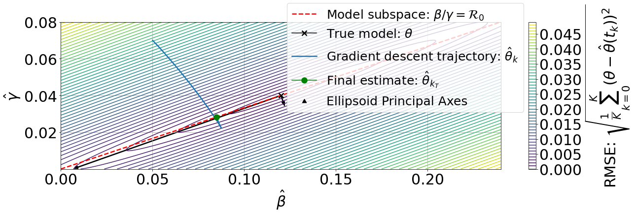
(a) Error contour and estimation trajectory

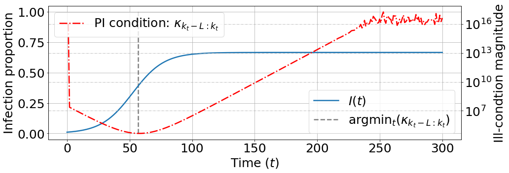
(b) Measured output and PI condition

Figure 1: The trajectory of $\hat{\theta}_{k}$ on the RMSE contour plot is shown in Fig. 1(a) for a noiseless SIS model $(\beta=0.12$, $\gamma=0.04$, $I(0)=0.01$, $\hat{\beta}_{k_{0}}=0.05$, $\hat{\gamma}_{k_{0}}=0.07)$. The red dotted line in Fig. 1(a) is the subspace of parameters characterized by the same reproduction number $\beta/\gamma$. We choose the signal length $L=2$ for computing the PI condition in Fig. 1(b).

Instead, the estimator $\hat{\theta}_{k}$ gravitates towards the model subspace defined by the reproduction number $\mathcal{R}_{0}=\beta/\gamma>1$, as denoted by the red dotted line in Fig. 1(a). This phenomenon implies an alternative reparameterization $(\tilde{\theta},\tilde{\phi},\tilde{\psi})$ of (13) that is robust against rank deficiency near $I_{*}$ is needed.

In Fig. 1(b), the moving PI condition $\kappa_{k_{t}-L:k_{t}}$ as defined in Definition 6, with signal duration of $L=2$ attains its minimum at $t=57$. Subsequently, $\kappa_{k_{t}-L:k_{t}}$ increases monotonically until the information matrix loses its invertibility after $t=250$. This phenomenon suggests that the information carried by $\{\phi_{k}\}$ can be decomposed into the transient and the steady-state components. Furthermore, transient information persists only for the initial period between $t=[0,100]$ and reaches its peak at $t=57$, as we observe in Fig. 1(b). Once the system shifts from the transient phase to the steady-state, transient excitation is lost and the associated information matrix becomes ill-conditioned.

III Greedily Weighted Recursive Least Squares

Within the context of online parameter estimation, one of the issues that we face is the insufficient richness of the information provided by the input and output trajectory. Traditional solutions to the problem involve injecting exciting signals into the inputs. However, some other studies suggest that properly forgetting/remembering information in the past will help alleviate the diminishing richness of signal information over time[33]. This section delves into the challenges of diminishing information richness by analyzing the lack of persistent excitation and poor practical identifiability problems. We propose a solution to the above problems based on the notion of an excitation set.

III-A Excitation Set

One natural solution to the lack of PE and PI problems in Example 1 is to incorporate second-order information when computing the descent direction upon the arrival of every new data point. We introduce the following modification to the exponential forgetting recursive least squares (EF-RLS) algorithm. The proposed algorithm is detailed in Algorithm 1, and we refer to it as the Greedily-weighted Recursive Least Squares (GRLS) Algorithm. We now introduce the notion of the optimal excitation set and the greedy excitation set to illustrate the workings of the GRLS Algorithm.

Definition 7 (Optimal Excitation Set).

A subset of data points $\mathcal{E}$ in $\mathcal{D}_{K}=\{k\in\mathbb{Z}:k_{0}\leq k\leq K\}$ is optimally exciting if:

$$\mathcal{E}_{\text{opt}}(K)=\underset{\begin{subarray}{c}E\subseteq\mathcal{D}_{K}\end{subarray}}{\arg\min}\ \kappa\Big{(}\sum_{k\in E}\phi_{k}^{\top}\phi_{k}\Big{)}.$$

Similarly, we define the greedy excitation set for a streamlined approximation of its optimal counterpart.

Definition 8 (Greedy Excitation Set).

The $K^{th}$ data point belongs to the greedy excitation set $\mathcal{E}_{\text{g}}(K)$ if it does not deteriorate the Hessian’s condition number induced by $\mathcal{E}_{\text{g}}(K-1)$:

$$\kappa\Big{(}\sum_{\begin{subarray}{c}k\in\mathcal{E}_{\text{g}}(K-1)\\ \bigcup\{K\}\end{subarray}}\phi_{k}^{\top}\phi_{k}\Big{)}\leq\kappa\Big{(}\sum_{k\in\mathcal{E}_{\text{g}}(K-1)}\phi_{k}^{\top}\phi_{k}\Big{)}.$$

Moving onward, we investigate the possibility of implementing a greedy excitation set with the EF-RLS in the next section.

III-B Excitation Set Based Recursive Least Squares

The main modification of Algorithm 1 in the EF-RLS filtering lies in its strategy to preserve data points from the optimally exciting set, ensuring they remain undiluted by subsequent less-informative data. Since solving for the optimal excitation set at each update iteration is expensive, we propose a recursively feasible approach to approximate the optimally exciting set through a greedy excitation set. The pseudo-code for GRLS is provided below:

Algorithm 1 Greedily-weighted Recursive Least Squares

1:Initialize:

2:      $H^{(e)}_{0}$, $P_{0}$, $\hat{\theta}_{0}$, $\Phi^{(e)}_{0}$, $\upsilon^{(e)}_{0}$.

3:Inputs:

4:      Input datum $(\phi_{k},\psi_{k})$

5:if $k>0$ then

6:     $H^{(e)}\leftarrow H^{(e)}_{k-1}+\phi_{k}^{\top}\phi_{k}$

7:     if $\kappa(H^{(e)})\leq\kappa{(H^{(e)}_{k-1})}$ then

8:         $\Phi^{(e)}_{k},H^{(e)}_{k}\leftarrow[{\Phi^{(e)}_{k-1}}^{\top},\phi_{k}^{\top}]^{\top},H^{(e)}$

9:         $\upsilon^{(e)}_{k}\leftarrow\upsilon^{(e)}_{k-1}+\phi_{k}^{\top}\psi_{k}$

10:         $\Phi\leftarrow(\sqrt{1-\alpha})\Phi^{(e)}_{k}$

11:         $H,\upsilon\leftarrow(1-\alpha)H^{(e)}_{k},(1-\alpha)\upsilon^{(e)}_{k}$

12:     else

13:         $\Phi^{(e)}_{k},H^{(e)}_{k},\upsilon^{(e)}_{k}\leftarrow\Phi^{(e)}_{k-1},H^{(e)}_{k-1},\upsilon^{(e)}_{k-1}$

14:         $\Phi\leftarrow[(\sqrt{1-\alpha}){\Phi^{(e)}_{k}}^{\top},\phi_{k}^{\top}]^{\top}$

15:         $H\leftarrow(1-\alpha)H^{(e)}_{k}+\phi_{k}^{\top}\phi_{k}$

16:         $\upsilon\leftarrow(1-\alpha)\upsilon^{(e)}_{k}+\phi_{k}^{\top}\psi_{k}$

17:     end if

18:     $P_{k}\leftarrow\frac{1}{\alpha}P_{k-1}(I-{\Phi}^{\top}(\alpha I+\Phi P_{k-1}\Phi^{\top})^{-1}\Phi P_{k-1})$

19:     $\hat{\theta}_{k}\leftarrow\hat{\theta}_{k-1}+P_{k}(\upsilon-H\hat{\theta}_{k-1})$

20:end if

In words, the GRLS Algorithm can be summarized as follows: first, Lines 6-17 in Algorithm 1 update the greedy exciting set and the corresponding hyper-parameters for computing $\hat{\theta}_{k+1}$ upon every incoming datum. Second, if $\kappa(H^{(e)})\leq\kappa{(H^{(e)}_{k-1})}$, then we update the regressor matrices $\Phi^{(e)}_{k}$, the Hessian $H^{(e)}_{k}$ and the corrector term $\upsilon^{(e)}_{k}$ of the excitation set on Lines 8-9; else, $\Phi^{(e)}_{k},H^{(e)}_{k},\upsilon^{(e)}_{k}$ remain unchanged as specified in Line 10. Lastly, Lines 10-11, 14-16 use $\Phi^{(e)}_{k},H^{(e)}_{k},\upsilon^{(e)}_{k}$ to compute $\Phi,H,\upsilon$ which are needed for computing the inverse Hessian matrix $P_{k}$ and the new estimate $\hat{\theta}_{k}$. Note that the condition number can be recursively estimated, as detailed in [34], to fully streamline Algorithm 1. We are ready to characterize the optimality of Algorithm 1.

Theorem 2.

If $P_{0}$ is positive definite, then for all $k\in[0,\infty)$, $\hat{\theta}_{k+1}$ obtained by Algorithm 1 is the the unique minimizer of the cost function:

$$C_{k}=\sum_{i=0}^{k}w_{i,k}\|r_{i}(\hat{\theta}_{k})\|^{2}+\alpha^{k+1}\|\hat{\theta}_{k}-\theta_{0}\|_{P_{0}^{-1}}^{2}$$ (15)

with the weighting function defined as:

$$w_{i,k}=\begin{cases}(1-\alpha)\sum_{l=i}^{k}\alpha^{k-l}&\text{if $i\in\mathcal{E}_{\text{g}}(k)$,}\\ \alpha^{k-i}&\text{otherwise}.\end{cases}$$ (16)

Proof.

The proof leverages mathematical induction to proceed, and it suffices to show the inductive step. We first note that $C_{k}(\hat{\theta})$ can be written in terms of: $C_{k}(\hat{\theta})=\hat{\theta}^{\top}A_{k}\hat{\theta}+2b_{k}^{\top}\hat{\theta}+c_{k}$, where $A_{k},b_{k},c_{k}$ are:

$$A_{k} :=\sum_{i=0}^{k}w_{i,k}\phi_{i}^{\top}\phi_{i}+\alpha^{k+1}P^{-1}_{0}$$

$$b_{k} :=-\sum_{i=0}^{k}w_{i,k}\phi_{i}^{\top}\psi_{i}-\alpha^{k+1}P^{-1}_{0}\theta_{0}$$

$$c_{k} :=\sum_{i=0}^{k}w_{i,k}\psi_{i}^{\top}\psi_{i}+\alpha^{k+1}\theta_{0}^{\top}P^{-1}_{0}\theta_{0}.$$

Then, $A_{k},b_{k}$ can be computed recursively as

$$A_{k} =\alpha A_{k-1}+\sum_{i\in U}\omega_{i}\phi_{i}^{\top}\phi_{i}$$

$$b_{k} =\alpha b_{k-1}-\sum_{i\in U}\omega_{i}\phi_{i}^{\top}\psi_{i},$$

where $U=\mathcal{E}_{\text{g}}(k)\bigcup\{k\}$, and $\omega_{i}=\begin{cases}(1-\alpha)&\text{if $i\in\mathcal{E}_{\text{g}}(k)$},\\ 1&\text{otherwise}.\end{cases}$ By way of induction, assume $\exists~{}k\in\mathbb{N}$ such that $A_{k-1}$ is positive definite and the unique optimizer of $C_{k-1}$ is $\hat{\theta}_{k}=-A_{k-1}^{-1}b_{k-1}$. We define $P_{k+1}:=A_{k}^{-1}$. Since $A_{k-1}$ is positive definite, we can apply the matrix inversion lemma[35, p, 304] and obtain a positive definite $P_{k+1}$:

$$P_{k+1} =A_{k}^{-1}$$

$$=\frac{1}{\alpha}\left(A_{k-1}+\frac{1}{\alpha}\left(\sum_{i\in U}\omega_{i}\phi_{i}^{\top}\phi_{i}\right)\right)^{-1}$$

$$=\frac{1}{\alpha}P_{k}-\frac{1}{\alpha}P_{k}{\Phi}^{\top}(\alpha I+\Phi P_{k}\Phi^{\top})^{-1}\Phi P_{k},$$

where $\Phi=\begin{cases}(\sqrt{1-\alpha})\Phi^{(e)}_{k+1}&\text{if $k\in\mathcal{E}_{\text{g}}(k)$,}\\ [(\sqrt{1-\alpha})(\Phi^{(e)}_{k+1})^{\top},\phi_{k}^{\top}]^{\top}&\text{otherwise},\end{cases}$ and $\Phi^{(e)}_{k+1}=\begin{bmatrix}\phi_{k_{1}}^{\top},\phi_{k_{2}}^{\top},\dots,\phi_{k_{r}}^{\top}\end{bmatrix}_{k_{i}\in\mathcal{E}_{\text{g}}(k)}^{\top}$, which satisfies the computation of $\Phi^{(e)}_{k+1}$ and $\Phi$ on Lines 8, 10, 13, and 14 of Algorithm 1. By the quadratic minimization lemma [35], the unique minimizer of $C_{k}(\hat{\theta})$ is:

$$\hat{\theta}_{k+1} =-A_{k}^{-1}b_{k}$$

$$=A_{k}^{-1}\Big{(}-\alpha b_{k-1}+\sum_{i\in U}\omega_{i}\phi_{i}^{\top}y_{i}\Big{)}$$

$$=A_{k}^{-1}\Big{(}\alpha A_{k-1}\hat{\theta}_{k}+\sum_{i\in U}\omega_{i}\phi_{i}^{\top}y_{i}\Big{)}$$

$$=A_{k}^{-1}\Big{(}\Big{(}A_{k}-\sum_{i\in U}\omega_{i}\phi_{i}^{\top}\phi_{i}\Big{)}\hat{\theta}_{k}+\sum_{i\in U}\omega_{i}\phi_{i}^{\top}y_{i}\Big{)}$$

$$=\hat{\theta}_{k}+A_{k}^{-1}\Big{(}\sum_{i\in U}\omega_{i}\phi_{i}^{\top}\psi_{i}-\Big{(}\sum_{i\in U}\omega_{i}\phi_{i}^{\top}\phi_{i}\Big{)}\hat{\theta}_{k}\Big{)}$$

$$=\hat{\theta}_{k}+P_{k+1}(\upsilon-H\hat{\theta}_{k}),$$

where $\upsilon:=\sum_{i\in U}\omega_{i}\phi_{i}^{\top}\psi_{i}$ and $H:=\sum_{i\in U}\omega_{i}\phi_{i}^{\top}\phi_{i}$ matches the computation of $\upsilon$ and $H$ on Lines 11, 15, and 16 of Algorithm 1. By the principle of mathematical induction, $P_{n}$ is positive definite, and $\hat{\theta}_{n+1}$ is the unique minimizer of $C_{n}$ for all $n\in\mathbb{N}$. ∎

While Theorem 2 characterizes the cost function which Algorithm 1 optimizes, the structure of the weighting function $w_{i,k}$ might not be immediately obvious. The intuition of the choice of $w_{i,k}$ becomes apparent when considering its asymptotic behavior, as established below.

Corollary 2.1.

If $P_{0}$ is positive definite and all $x\in\lim_{k\to\infty}\mathcal{E}_{g}(k)$ are obtained before $k=K$, for some $K<\infty$, and $\alpha<1$, then, as $k\to\infty$, $\hat{\theta}_{k+1}$ obtained by Algorithm 1 is the the unique minimizer of the cost function:

$$C_{k}(\hat{\theta})=\sum_{i=0}^{k}W_{i,k}\|r_{i}(\hat{\theta})\|^{2},$$ (17)

with

$$W_{i,k}=\begin{cases}1&\text{if $i\in\mathcal{E}_{g}(K)$}\\ \alpha^{k-i}&\text{otherwise}.\end{cases}$$ (18)

Proof.

Note that, since $\alpha<1$, the second term in the cost function in (15), $\alpha^{k+1}\|\hat{\theta}-\theta_{0}\|_{P_{0}^{-1}}^{2}$, goes to zero as $k\to\infty$. Furthermore, $\sum_{l=i}^{k}\alpha^{k-l}$ can be rewritten as $\sum_{l=0}^{k-i}\alpha^{l}$, and since $\sum_{l=0}^{k-i}\alpha^{l}$ is a geometric sum, $\lim_{k\to\infty}(1-\alpha)\sum_{l=i}^{k}\alpha^{k-l}=1$. Thus, the weighting function $w_{i,k}$ can be written as $W_{i,k}$ in (18). Therefore, by Theorem 2, Algorithm 1 obtains the optimal $\theta^{*}={\arg\min}_{\hat{\theta}}C_{k}(\hat{\theta})$ for the simplified cost function in (17)-(18). ∎

Corollary 2.1 characterizes the asymptotic behavior of the cost function which Algorithm 1 minimizes. The algorithm stores the data points that belong to the greedy excitation set by giving them a weight of $1$ while assigning the unexciting points exponentially decaying weights. Lastly, we end this section with a note on the structure of the closed-form solution of the GRLS algorithm.Let $\mathbf{w}_{k}=[w_{0,k},\dots,w_{k,k}]^{\top}$ be the vector form of the weight function (16).

Corollary 2.2.

The unique optimal solution $\hat{\theta}_{k}$ to the cost function (15) has the closed-form expression:

$$\hat{\theta}_{k}=(\Phi_{k}^{\top}\mathbf{W}_{k}\Phi_{k}+R_{k})^{-1}(\Phi_{k}^{\top}\mathbf{W}_{k}\Psi_{k}+R_{k}\theta_{0}),$$ (19)

where $R_{k}=\alpha^{k+1}P^{-1}_{0}$, $\Psi_{k}=\begin{bmatrix}\psi_{0}^{\top},\dots,\psi_{k}^{\top}\end{bmatrix}^{\top}$, and $\mathbf{W}_{k}=\text{diag}(\mathbf{w}_{k})\otimes I_{n}.$

Proof.

Let $R_{k}=\alpha^{k+1}P^{-1}_{0}$, we can rewrite the cost function (15) in matrix form:

$$C_{k}(\hat{\theta}_{k})=(\Psi_{k}-\Phi_{k}\hat{\theta}_{k})^{\top}\mathbf{W}_{k}(\Psi_{k}-\Phi_{k}\hat{\theta}_{k})+(\hat{\theta}_{k}-\theta_{0})^{\top}R_{k}(\hat{\theta}_{k}-\theta_{0}).$$

Then we can take the partial derivative of $C_{k}(\hat{\theta}_{k})$ with respect to $\hat{\theta}_{k}$ and set the partials to zeros, which yield the desired result:

$$0 =-2\Psi_{k}\mathbf{W}_{k}X+2\Phi_{k}^{\top}\Phi_{k}\hat{\theta}_{k}+2R_{k}\hat{\theta}_{k}-2R_{k}\theta_{0}$$

$$\hat{\theta}_{k} =(\Phi_{k}^{\top}\mathbf{W}_{k}\Phi_{k}+R_{k})^{-1}(\Phi_{k}^{\top}\mathbf{W}_{k}\Psi_{k}+R_{k}\theta_{0}).$$

This concludes the proof. ∎

The above result comes naturally from the observation that the minimization problem with respect to the cost (15) is a weighted ridge least square problem. The bias term $R_{k}\theta_{0}$ vanishes when $k$ is sufficiently large. These observations will assist us in analyzing the prediction errors in the next section.

IV Hyper-Parameters Resetting with Change Point Detection

In this section, we are interested in handling time-varying systems with piecewise constant parameters in time. We design a change point detection algorithm that detects jumps in $\theta(t_{k})$ when the predictive ability of the estimated parameter vector $\hat{\theta}_{k}$ deteriorates. Once a jump is detected, the estimator memory is reinitialized, in order to avoid estimation errors from incorporating outdated data points which originated from irrelevant parameters in the past.

IV-A Prediction Error Dynamics

We define the prediction residual $e_{k}\coloneqq\psi_{k}-\phi_{k}\hat{\theta}_{k-1}$ and prediction error $\|e_{k}\|^{2}$ to quantify the predictability of the estimated parameter vector $\hat{\theta}_{k-1}$. Assuming that $\xi_{k}$ in (2) is an i.i.d. Gaussian random variable, $\xi_{k}\sim\mathcal{N}(0,\sigma^{2}I)$, the behavior of $e_{k}$ for the class of online estimation algorithms that solve for the weighted ridge least squares solution in (19) is provided in the following proposition.

Proposition 1.

If the error terms $\xi_{k}\sim\mathcal{N}(0,\sigma^{2}I_{n})$ are i.i.d. Gaussian random variables, then the prediction residual $e_{k}=\psi_{k}-\phi_{k}\hat{\theta}_{k-1}$ of the estimator $\hat{\theta}_{k}$ in the form of (19) follows the Gaussian distribution $\mathcal{N}(\mu_{k},\sigma^{2}A_{k}A_{k}^{T})$, where $\mu_{k},A_{k}$ are defined as:

$$\mu_{k} \coloneqq\phi_{k}(R^{-1}_{k-1}\Phi_{k-1}^{\top}\mathbf{W}_{k-1}\Phi_{k-1}+I)^{-1}(\theta(t_{k})-\theta_{0}),$$

$$A_{k} \coloneqq[-\phi_{k}(\Phi_{k-1}^{\top}\mathbf{W}_{k-1}\Phi_{k-1}+R_{k-1})^{-1}\Phi_{k-1}^{\top}\mathbf{W}_{k-1},\ I].$$

Proof.

We proceed by deriving the closed-form expression of $e_{k+1}$. We leverage the closed-form expression of $\hat{\theta}_{k}$ in (19) in the following derivation:

$$e_{k+1}= \psi_{k+1}-\phi_{k+1}\hat{\theta}_{k}$$

$$= \phi_{k+1}(\theta(t_{k+1})-\hat{\theta}_{k})+\xi_{k+1}$$

$$= \phi_{k+1}[(\Phi_{k}^{\top}\mathbf{W}_{k}\Phi_{k}+R_{k})^{-1}(\Phi_{k}^{\top}\mathbf{W}_{k}\Phi_{k}+R_{k})\theta(t_{k+1})$$

$$\ \ -(\Phi_{k}^{\top}\mathbf{W}_{k}\Phi_{k}+R_{k})^{-1}(\Phi_{k}^{\top}\mathbf{W}_{k}\Psi_{k}+R_{k}\theta_{0})]+\xi_{k+1}$$

$$= \phi_{k+1}(\Phi_{k}^{\top}\mathbf{W}_{k}\Phi_{k}+R_{k})^{-1}[(\Phi_{k}^{\top}\mathbf{W}_{k}(\Phi_{k}\theta(t_{k+1})-\Psi_{k})$$

$$\ \ +R_{k}(\theta(t_{k+1})-\theta_{0}))]+\xi_{k+1}$$

$$= -\phi_{k+1}(\Phi_{k}^{\top}\mathbf{W}_{k}\Phi_{k}+R_{k})^{-1}\Phi_{k}^{\top}\mathbf{W}_{k}\text{vec}_{0:k}(\xi_{i})+\xi_{k+1}$$

$$\ \ +\phi_{k+1}(\Phi_{k}^{\top}\mathbf{W}_{k}\Phi_{k}+R_{k})^{-1}R_{k}(\theta(t_{k+1})-\theta_{0})$$

$$= A_{k+1}\cdot\text{vec}_{0:k+1}(\xi_{i})+\mu_{k+1},$$

where

$$A_{k+1} \coloneqq[-\phi_{k+1}(\Phi_{k}^{\top}\mathbf{W}_{k}\Phi_{k}+R_{k})^{-1}\Phi_{k}^{\top}\mathbf{W}_{k},\ I]$$

$$\mu_{k+1} \coloneqq\phi_{k+1}(R^{-1}_{k}\Phi_{k}^{\top}W_{k}\Phi_{k}+I)^{-1}(\theta(t_{k+1})-\theta_{0}).$$

The second to third step is possible through invertibility of $\Phi_{k}^{\top}\mathbf{W}_{k}\Phi_{k}+R_{k}$, and because $\hat{\theta}_{k}=\Phi_{k}^{\top}\mathbf{W}_{k}\Phi_{k}+R_{k})^{-1}(\Phi_{k}^{\top}\mathbf{W}_{k}\Psi_{k}+R_{k}\theta_{0})$ by assumption. The forth to fifth step is possible because $\text{vec}_{0:k}(\xi_{i})=\Psi_{k}-\Phi_{k}\theta$, by (2). Furthermore, since $\xi_{i}\sim\mathcal{N}(0,\sigma^{2}I_{n})$ are i.i.d. zero-mean Gaussian, $e_{k+1}$ is a multi-variate Gaussian vector with $\mathbb{E}\{e_{k+1}\}=\mu_{k+1}$ and $\mathrm{Cov}(e_{k+1})=\sigma^{2}A_{k+1}A_{k+1}^{\top}\eqqcolon\Sigma_{k+1}$. Replacing $k+1$ by $k$ yields the desired result. ∎

Therefore, we can see that the prediction residual $e_{k}$ is a stochastic process with time-varying means and variances. Consequently, the transformed prediction error, $\|e_{k}-\mu_{k}\|^{2}_{\Sigma^{-1}_{k}}$, follows a $\chi_{2}$ distribution.

To summarize, $\|e_{k}\|^{2}$ is a signal dependent on the past data $\Phi_{k}$, the true parameters $\theta(t_{k})$, and some hyper-parameters $\theta_{0}$ and $W_{k}$ specific to an online estimator under the Gaussian noise assumption. Additionally, we expect to observe a change in $\mu_{k}$ during abrupt changes in $\theta(t_{k})$ because it is a function of $\theta(t_{k})$, the new data point $\phi_{k+1}$, and the past data points $\Phi_{k}$. Lastly, since the prediction error spans several orders of magnitude, we apply a negative logarithmic transformation to $\|e_{k}\|^{2}$ to define the notion of model predictability.

Definition 9.

The model predictability at time $t_{k}$ is defined as $Y_{k}\coloneqq-\log(\|e_{k}\|^{2})$, where $e_{k}\coloneqq\psi_{k}-\phi_{k}\hat{\theta}_{k-1}$.

The model predictability $Y_{k}\in(-\infty,\infty)$ is the negative order of magnitude of the prediction error. While its value may depend on the application, a high $Y_{k}$ indicates good performance of the upstream online estimator.

We aim to create a versatile framework for identifying change points and adjusting hyper-parameters that is effective for different online estimators and under multiple noise conditions. Based on the analysis of incoming prediction errors, we model the stochastic process $\{Y_{k}\}$ with an exponentially weighted average model (EWAM) [17]:

$$Z_{k}=\alpha Y_{k}+(1-\alpha)Z_{k-1},~{}Z_{0}\coloneqq Y_{1},$$ (20)

where $\alpha\in[0,1]$ is an exponential weighting term. We can use the $m$-lagged EWAM, $Z_{k-m}$, as a predictor of the current $Y_{k}$. Therefore, the estimator of $Y_{k}$ is computed as:

$$\hat{Y}_{k}(m)=Z_{k-m}.$$

The $m$-lagged EWAM estimator effectively acts as a low pass filter on $\mathbf{Y}\coloneqq\{Y_{k}\}$. If $Y_{k}$ deviates too much from $\hat{Y}_{k}(m)$, it is a good sign of a change point occurrence. The following example demonstrates the interplay between a time-varying system, model predictability, and the EWAM estimator.

Example 2.

Consider a 2-node susceptible-infected-recovered (SIR) system:

$$\dot{I}(t) =\text{diag}(1-I(t)-R(t))B(t)I(t)-\text{diag}(\gamma(t))I(t)$$ (21)

$$\dot{R}(t) =\text{diag}(\gamma(t))I(t),$$

where $I\in[0,1]^{2}$ is the infected proportion, $R\in[0,1]^{2}$ is the recovered proportion, $B\in\mathbb{R}_{\geq 0}^{2}\times\mathbb{R}^{2}_{\geq 0}$ is the infection rate matrix, and $\gamma\in\mathbb{R}_{\geq 0}^{2}$ is the vector of recovery rates. The system parameters $B$ and $\gamma$ are time-varying but remain piece-wise constant, emulating the lockdown effects and rebound in social activity during the reopening period.

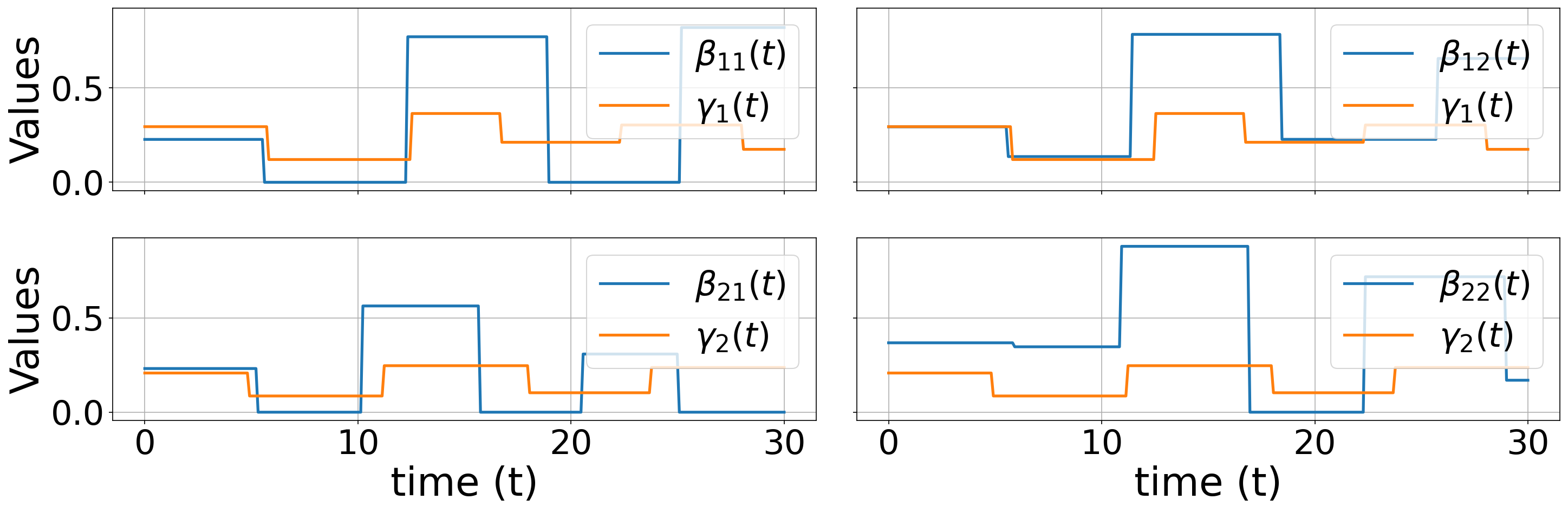
Figure 2: Time-varying parameters of a 2-node SIR network

Fig. 2 visualizes the time-varying parameters. Let $R,I$, and their derivatives be observable; we can fit the data through an EF-RLS algorithm. A visualization of the evolution of ${Y_{k}}$ in conjunction with its 1-lagged EWAM estimator $Z_{k-1}$ is shown in Fig. 3.

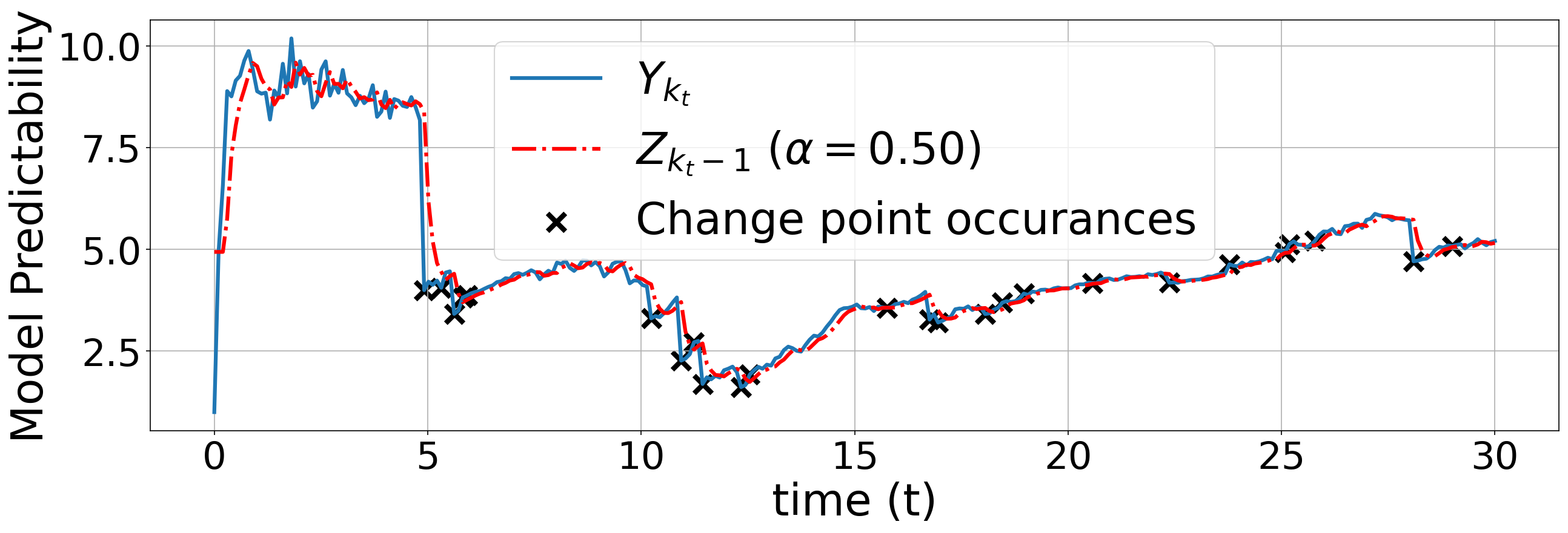
Figure 3: Evolving model predictability of an EF-RLS and its 1-lagged EWAM ($\alpha=0.5$) estimation.

From Fig. 3, it is evident that a significant upward trend in $Y_{k}$ occurs during the initial training phase until reaching the first change point, marked by the black crosses. Subsequently, $Y_{k}$ persists at a lower value due to the effect of outdated data points in the inferred covariance matrix, stemming from previous $\theta(t_{k})$ values.

IV-B Change Point Detection

In this subsection, we design a simple recursive likelihood ratio test to detect change point occurrences. A draft of the two hypotheses can be constructed as follows to test for change points in $\theta(t)$:

• $\bar{H}_{0}$: The stochastic process $\{Y_{i}\}_{k_{1}:k_{2}}$ is “captured” by a single EWAM.

• $\bar{H}_{1}$: The stochastic process $\{Y_{i}\}_{k_{1}:k_{2}}$ is “captured” by two EWAMs, residing in two intervals $[k_{1},k_{c}]$ and $[k_{c}+1,k_{2}]$,

where $k_{1}\leq k_{c}\leq k_{2}$. In the context of our change point detection problem, it is advantageous to set $k_{c}=k_{2}-1$ because we want to prevent the most recent abnormal observation from impacting the upstream estimation process and EWAM value. Furthermore, we pick the lag value $m=1$, and write $\hat{Y}_{k}\coloneqq\hat{Y}_{k}(1)=Z_{k-1}.$

To clarify the meaning of “captured,” we need to establish a criterion that defines the cost of $\hat{Y}_{k}$ failing to predict $Y_{k}$ in the context of the detection problem. Let $\mathcal{S}_{k_{1}:k_{2}}\coloneqq\{k_{1},\dots,k_{2}\}$ be the index set of all residuals. The set $\mathcal{S}_{k_{1}:k_{2}}$ is then partitioned into two residual index sets: the positive, $\mathcal{S}_{k_{1}:k_{2}}^{+}\coloneqq\{k:\hat{Y}_{k}-Y_{k}>0,k_{1}\leq k\leq k_{2}\}$, and non-positive, $\mathcal{S}_{k_{1}:k_{2}}^{-}=\{k:\hat{Y}_{k}-Y_{k}\leq 0,k_{1}\leq k\leq k_{2}\}$. After fixing an exponential weight $\alpha$, the cost of $\hat{Y}_{k}$ failing to predict is defined below.

Definition 10.

The Mean Positive Square Error (MPSE) is defined as the conditional expectation of $\hat{Y}_{k}-Y_{k}$ on the set $\mathcal{S}^{+}$:

$$\text{MPSE}(\mathbf{Y})=\mathbb{E}[(\hat{Y}_{k}-Y_{k})^{2}|k\in\mathcal{S}^{+}].$$

When there is an abrupt change, it results in $Y_{k}<\hat{Y}_{k}$ and an increase in $\|e_{k}\|^{2}$, consistent with the objective of our task. However, note that the distribution of $\hat{Y}_{k}-Y_{k}$ after the partition can no longer assumed to be Gaussian, and a generalized error distribution should be considered when computing the likelihood. To simplify computation of the likelihood, we make the following assumption on the distribution of $\hat{Y}_{k}-Y_{k}$.

Assumption IV.1.

Let $E_{k}\coloneqq(\hat{Y}_{k}-Y_{k})^{2}$, where $k\in\mathcal{S}^{+}$, be independent and identically distributed (i.i.d.) exponential random variables, that is, $E_{k}|\mathcal{S}^{+}\sim\text{Exp}(\lambda)$.

Fig. 4 visualizes the distribution of residuals from $\mathcal{S}^{+}$ under Example 2.

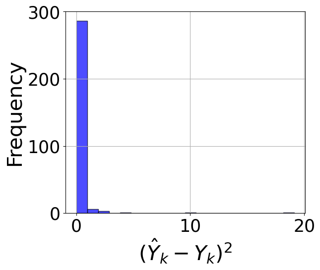
Figure 4: Histogram of the squared positive residuals set, $\mathcal{S}^{+}=\{k:\hat{Y}_{k}-Y_{k}>0,0\leq k\leq 300\}$.

With a slight abuse of notation, we define $\text{MPSE}(\{E_{i}\}_{k_{1}:k_{2}})\coloneqq\mathbb{E}[E_{k}|k\in\mathcal{S}_{k_{1}:k_{2}}^{+}].$ Then, under Assumption IV.1, the null and alternative hypotheses for the likelihood ratio test can be constructed as follows:

• $H_{0}$: $E_{i}|\mathcal{S}^{+}\sim\text{Exp}(\lambda_{0})~{}\forall k_{1}\leq i\leq k_{2}$

• $H_{1}$: $E_{i}|\mathcal{S}^{+}\sim\text{Exp}(\lambda_{1})~{}\forall k_{1}\leq I<k_{2}$
  and $E_{k_{2}}|\mathcal{S}^{+}\sim\text{Exp}(\lambda_{2})$

where $\lambda_{0}^{-1}=\text{MPSE}(\{E_{i}\}_{k_{1}:k_{2}})$ and $\lambda_{1}^{-1}=\text{MPSE}(\{E_{i}\}_{k_{1}:k_{2}-1})$ and are estimated by computing the sample mean of $E_{k}|\mathcal{S}^{+}_{k_{1}:k_{2}}$ and $E_{k}|\mathcal{S}^{+}_{k_{1}:k_{2}-1}$, respectively. However, note that since $\mathcal{S}^{+}_{k_{2}:k_{2}}$ is empty, the statement “$E_{k_{2}}|\mathcal{S}^{+}\sim\text{Exp}(\lambda_{2})$,” is vacuously true regardless of the value of $\lambda_{2}$. Therefore, the alternative hypothesis can be rewritten as $H_{1}$: $E_{i}|\mathcal{S}^{+}\sim\text{Exp}(\lambda_{1})~{}\forall k_{1}\leq i\leq k_{2}-1$.

Definition 11 (Likelihood Ratio Test Statistic).

Let $\mathbf{E}=\{E_{1},E_{2},\ldots,E_{n}\}$ be random samples from a probability distribution with parameters $\Lambda$. Suppose $\Lambda_{0}=\{\lambda_{0}^{1},\dots,\lambda_{0}^{d_{\text{null}}}\}$ is the set of the parameters under the null hypothesis, and let $\Lambda_{1}=\{\lambda_{1}^{1},\dots,\lambda_{1}^{d_{\text{alt}}}\}$ be the parameters set under the alternative hypothesis. The test statistic $D(\textbf{E})$ is defined as:

$$D(\textbf{E})=-2\ln\left(\frac{L(\textbf{E}|\Lambda_{0})}{L(\textbf{E}|\Lambda_{1})}\right)$$ (22)

where $L(\textbf{E}|\Lambda)$ is the likelihood function.

In the context of our problem, $d_{\text{null}}=1$ as the null hypothesis $H_{0}$ posits that the sequence $\{Y_{i}\}_{k_{1}:k_{2}}$ is represented by one EWAM, leading to a single exponential distribution $\exp(\lambda_{0})$. Similarly, $d_{\text{alt}}=2$ as a result of the alternative hypothesis $H_{2}$ positing that $\{E_{k}\}_{k_{1}:k_{2}}$ is generated by two exponential distributions. Then, with the choice of the test statistic $D$ induced from Assumption IV.1, we can recursively perform the likelihood ratio test (LRT) with threshold value $\tau$ leveraging Algorithm 2.

Algorithm 2 Recursive LRT for change point detection (rLRT)

1:Initialize:

2:      Error threshold: $\tau\in[0,1]$ Exponential weighting factor: $\alpha\in[0,1]$ Initial EWAM: $Z_{0}\leftarrow Y_{1}$ Initial residual mean: $\lambda_{0}\leftarrow 0$ Number of downward drifts: $n\leftarrow 0$

3:Inputs:

4:      Input datum: $Y_{k}$, Data count: $k$

5:if $k\geq 1$ then

6:     if $Z_{k-1}-Y_{k}>0$ then

7:         $E\leftarrow(Z_{k-1}-Y_{k})^{2}$

8:         $\lambda\leftarrow(n+1)/(\frac{n}{\lambda_{n}}+E)$

9:         $D\leftarrow 2\left(n\ln(\lambda_{n})-(n+1)\ln(\lambda)+1\right)$

10:         $p\leftarrow 1-\text{CDF}_{\chi^{2}}(D,1)$

11:         if $p\leq\tau$ then return True

12:         end if

13:         $n\leftarrow n+1$

14:         $\lambda_{n}\leftarrow\lambda$

15:     end if

16:     $Z_{k}\leftarrow\alpha Y_{k}+(1-\alpha)Z_{k-1}$

17:     Return False

18:end if

In Algorithm 2,

$$D=2\left(n\ln(\lambda_{n})-(n+1)\ln(\lambda)+1\right)$$

is the aforementioned test statistic. The properties of the hypothesis test follow naturally from the Wilks’ Theorem [36] and Neyman-Pearson Lemma [18], reproduced below for completeness.

Lemma 1 (Wilks’ Theorem [36]).

Under the null hypothesis $H_{0}$, the likelihood ratio test statistic $D(\textbf{E})$, as defined in (22) converges to the chi-squared distribution asymptotically in distribution as the number of random samples goes to infinity, that is:

$$D(\textbf{E})\overset{\text{dist}}{\to}\chi^{2}(d),$$ (23)

where the degree of freedom $d=d_{\text{alt}}-d_{\text{null}}$.

Lemma 2 (Neyman-Pearson Lemma [18, Thm. 8.6-1]).

Suppose there exists a positive constant $c$ and a subset $\mathcal{C}$ of the sample space such that:

1. $\text{Pr}[\textbf{E}\in\mathcal{C};\Lambda_{0}]=\tau$

2. $\frac{L(\textbf{E}|\Lambda_{0})}{L(\textbf{E}|\Lambda_{1})}\leq c~{}\text{ if }\textbf{E}\in\mathcal{C}$ and

3. $\frac{L(\textbf{E}|\Lambda_{0})}{L(\textbf{E}|\Lambda_{1})}>c~{}\text{ if }\textbf{E}\not\in\mathcal{C}$,

then $\mathcal{C}$ is the best critical region of size $\tau$ for testing the simple null hypothesis $H_{0}:\Lambda=\Lambda_{0}$ against the simple alternative hypothesis $H_{1}:\Lambda=\Lambda_{1}$.

In the context of our problem, the best critical region is a detection region of $D(\mathbf{E})$ that maximizes the probability of rejecting the null hypothesis when the alternative hypothesis is true for a given threshold value (significant level) $\tau$. With the key previous results stated, we are prepared to prove the following theorem for the properties of Algorithm 2.

Theorem 3.

Under Assumption IV.1, the hypothesis test $p\leq\tau$, has the following properties:

1. The test statistic:

   $$D(\mathbf{E})=2\left(n\ln(\lambda_{n})-(n+1)\ln(\lambda)+1\right)$$

   asymptotically converges to the chi-squared distribution $\chi^{2}(d)$ in distribution with $d=1$.

2. The likelihood ratio test $p\leq\tau$ maximizes the true positive rate (TPR) across all hypothesis tests of the same significant level $\tau$.

Proof.

Upon a new change point candidate $k_{2}$, where $E_{k_{2}}>0$, let $n=|\mathcal{S}^{+}_{k_{1}:k_{2}-1}|$; the sample mean of $\mathbf{E}|\mathcal{S}^{+}_{k_{1}:k_{2}-1}$ is computed as:

$$\lambda_{n}=\frac{n}{\sum_{k\in\mathcal{S}^{+}_{k_{1}:k_{2}-1}}E_{k}},$$ (24)

where $\lambda_{n}$ and $\lambda_{n+1}$ can be expressed in a recursive relationship, $\lambda_{n+1}=\frac{n+1}{\frac{n}{\lambda_{n}}+E_{k_{2}}},$ that aligns with the recursive update rule on line 6 in Algorithm 2. The log likelihood $\ln L(\mathbf{E}|\lambda_{1})$ is computed through the definition of the probability density function of an exponential distribution:

$$\ln L(\mathbf{E}|\Lambda_{1}) =\sum_{k\in\mathcal{S}^{+}_{k_{1}:k_{2}-1}}\ln(\lambda_{n}\exp(-\lambda_{n}E_{k}))$$

$$=\sum_{k\in\mathcal{S}^{+}_{k_{1}:k_{2}-1}}(\ln\lambda_{n}-\lambda_{n}E_{k})$$

$$=n\ln(\lambda_{n})-\lambda_{n}\sum_{k\in\mathcal{S}^{+}_{k_{1}:k_{2}-1}}E_{k}$$

$$=n\ln\lambda_{n}-n.$$

The likelihood of $H_{0}$, $L(\mathbf{E}|\Lambda_{0})$, is computed similarly through replacing $n$ by $n+1$. Let $\lambda\coloneqq\lambda_{n+1}$ to simplify notation. Then, the test statistic $D(\mathbf{E})$ can be evaluated as:

$$D(\mathbf{E}) =2\left(n\ln(\lambda_{n})-(n+1)\ln(\lambda)+1\right)$$

$$=-2((n+1)\ln\lambda-(n+1)-(n\ln\lambda_{n}-n))$$

$$=-2(\ln(L(\mathbf{E}|\Lambda_{0}))-\ln(L(\mathbf{E}|\Lambda_{1})))$$

$$=-2\left(\ln\frac{L(\mathbf{E}|\Lambda_{0})}{L(\mathbf{E}|\Lambda_{1})}\right),$$

which is in the form of likelihood ratio test statistic in Definition 11. By Lemma 1, the test statistic $D(\mathbf{E})\overset{\text{dist}}{\to}\chi^{2}(d)$, where the degree of freedom $d=d_{\text{alt}}-d_{\text{null}}=1$ by Definition 11. Moreover, the likelihood ratio test:

$$1-\text{CDF}_{\chi^{2}}(D(\mathbf{E}))\leq\tau$$ (25)

induces a critical region $\mathcal{C}=\{\mathbf{E}\in\Omega:\text{reject }H_{0}\text{ if }\mathbf{E}\in\mathcal{C}\}$ of size $\tau$. The sample $E_{k}\in\mathcal{C}$ if and only if (25) is satisfied. Since $\text{CDF}_{\chi^{2}}(\cdot)$ and $\ln(\cdot)$ are monotonic functions, we can rewrite (25):

$$~{}1-\text{CDF}_{\chi^{2}}(D(\mathbf{E}))\leq\tau$$

$$\Rightarrow D(\mathbf{E})\geq\text{CDF}_{\chi^{2}}^{-1}(1-\tau)$$

$$\Rightarrow \ln\left(\frac{L(\mathbf{E}|\Lambda_{0})}{L(\mathbf{E}|\Lambda_{1})}\right)\leq\frac{1}{2}\text{CDF}_{\chi^{2}}^{-1}(1-\tau)$$

$$\Rightarrow \frac{L(\mathbf{E}|\Lambda_{0})}{L(\mathbf{E}|\Lambda_{1})}\leq\exp\left(\frac{1}{2}\text{CDF}_{\chi^{2}}^{-1}(1-\tau)\right)\eqqcolon c.$$

The critical region $\mathcal{C}$ is the best among all hypothesis tests through Lemma 2. Therefore, $1-\text{CDF}_{\chi^{2}}(D(\mathbf{E}))\leq\tau$ is uniformly most powerful in this sense. ∎

Algorithm 2 maximizes the TPR, a.k.a. power, at a given significance level $\tau$. However, we have chosen the simple EWAM model and exponentially distributed error distribution to simplify the computation of the test statistic $D(\mathbf{E})$ in the recursive context of our problem. Therefore, the fulfillment of Assumption IV.1 may vary depending on the complexity of the online parameter estimator and the level of excitation of the upstream regressor signal.

The change point detection algorithm can be applied to all online estimation algorithms that retain some memory or state during their estimation process. By integrating the downstream change point algorithm, we can enhance their performance in a time-varying environment. Presented below is an algorithmic framework for incorporating the change point detection algorithm to facilitate online state resetting.

Algorithm 3 Change Point State Resetting Online Estimator

1:Initialize:

2:      Estimator Hyper-parameters: $\Psi$ Online Estimator State: $\mathcal{S}_{0}$ Parameter Estimate: $\hat{\theta}_{0}$ Online Estimator: $\hat{\theta}\leftarrow\hat{\theta}(\ \cdot\ ,\mathcal{S}_{0},\hat{\theta}_{0};\Psi)$

3:Inputs:

4:      Input datum: $(x_{k},y_{k})$, Data count: $k$

5:if $k\geq 1$ then

6:     $\hat{\theta}_{k},\mathcal{S}_{k}\leftarrow\hat{\theta}((x_{k},y_{k}),\mathcal{S}_{k-1},\hat{\theta}_{k-1})$

7:     $Y_{k}\leftarrow-\log(\|y_{k}-\phi(x_{k})\hat{\theta}_{k-1}\|_{2}^{2})$

8:     Run Algorithm 2: detectChange $\leftarrow$ rLRT($Y_{k}$)

9:     if detectChange then

10:         $\hat{\theta}\leftarrow\hat{\theta}(\ \cdot\ ,\mathcal{S}_{0},\hat{\theta}_{k})$

11:     else

12:         $\hat{\theta}\leftarrow\hat{\theta}(\ \cdot\ ,\mathcal{S}_{k},\hat{\theta}_{k})$

13:     end if

14:end if

For a exponentially forgetting recursive least squares algorithm, the state is the approximated covariance matrix, $\mathcal{S}=\{P_{k}\}$. In the case of the GWRLS, the states include the information of the excitation set $H^{(e)}_{k}$, the excitation set cross-correlation vector $\nu_{k}^{(e)}$, the excitation set $\Phi^{(e)}_{k}$, and the approximated covariance matrix $P_{k}$.

We may also consider the previously estimated parameter $\hat{\theta}_{k}$ as part of the estimator states if the system parameters deviate too much from its previous value after abrupt changes. In Section V, we investigate how the GRLS and change point detection algorithm impact the performance of an online estimator in both static and time-varying system identification problems.

V Simulations

This section aims to assess the performance of three algorithms: initially-excited multi-model adaptive identifier (IE-MMAI) [11], EF-RLS [2], and the newly proposed GRLS algorithm. We evaluate their effectiveness on the SIS and SIR networked compartmental models. Detailed discussions will be presented to offer insights into the disparities in performance, focusing on the practical identifiability and persistent excitation perspectives.

V-A SIS Compartmental Model

Consider the SIS compartmental dynamics:

$$dX(t)=d\phi_{\text{SIS}}(X(t))\theta dt+\sigma dW,$$ (26)

where $X(t)$ is the proportion of infected population, the parameter $\theta=[\beta,\ \gamma]^{\top}$, such that $\beta$ is the infection rate, $\gamma$ is the recovery rate, the regressor $\phi_{\text{SIS}}(X(t))=[X(t)(1-X(t)),\ -X(t)]$, and $W$ is the standard Wiener process. Note that (26) reduces to a deterministic ODE when the standard deviation $\sigma$ is set to zero.

We present parameter estimation results for both the noise-free case and including Gaussian process and observation noise for the SIS dynamics in (26). In Fig. 5, we compare the performance of IE-MMAI [11] and EF-RLS, to the performance of the GRLS Algorithm we propose. The same initial estimates of parameters, $\theta_{0}=[\beta_{0},\gamma_{0}]^{\top}=[1,1]^{\top}$, are used for all algorithms with the exception of IE-MMAI, for which the $m=3$ models were initialized randomly around $\theta_{0}$. The forgetting rate of EF-RLS and GRLS are set to $0.98$.

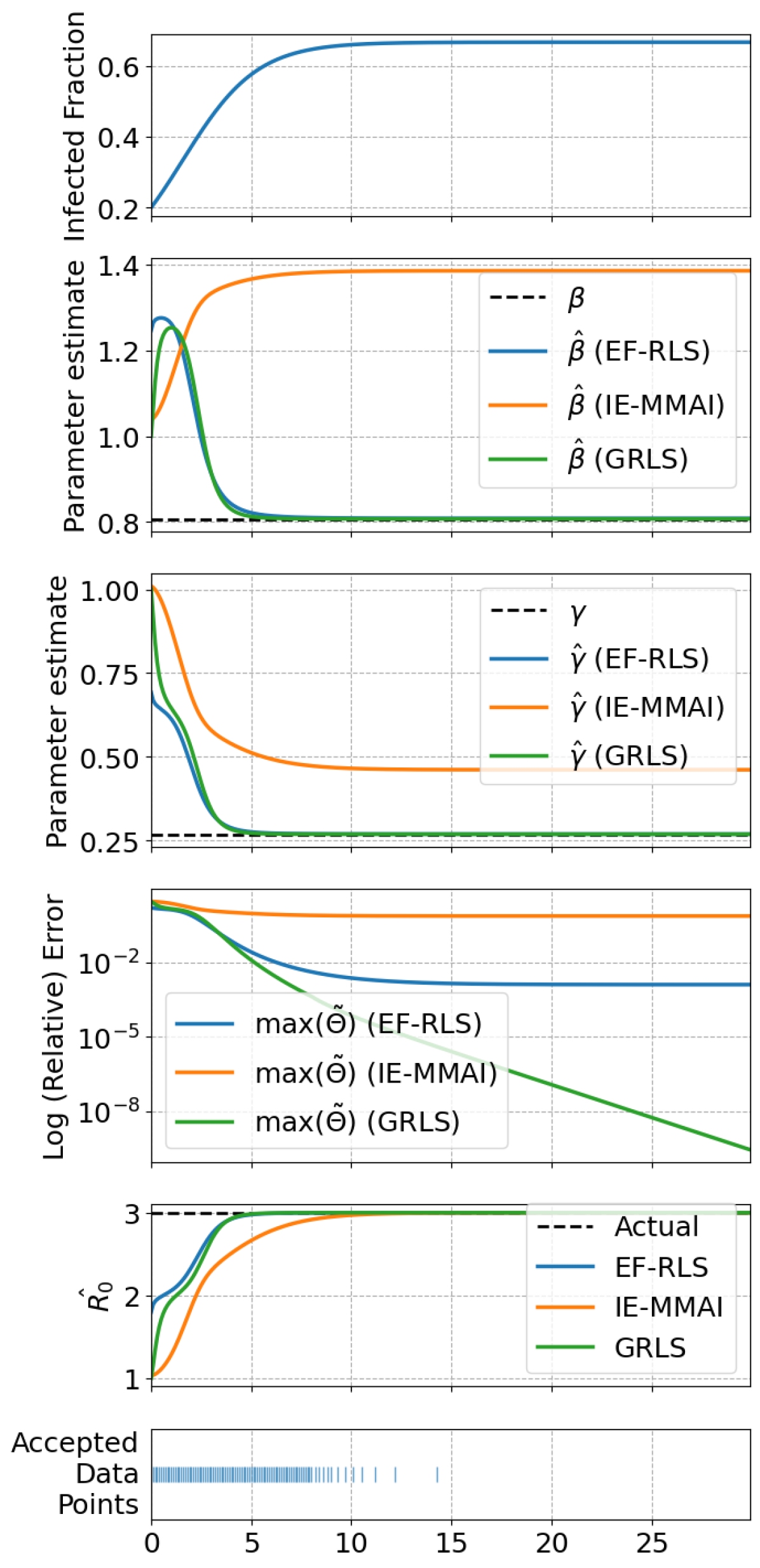
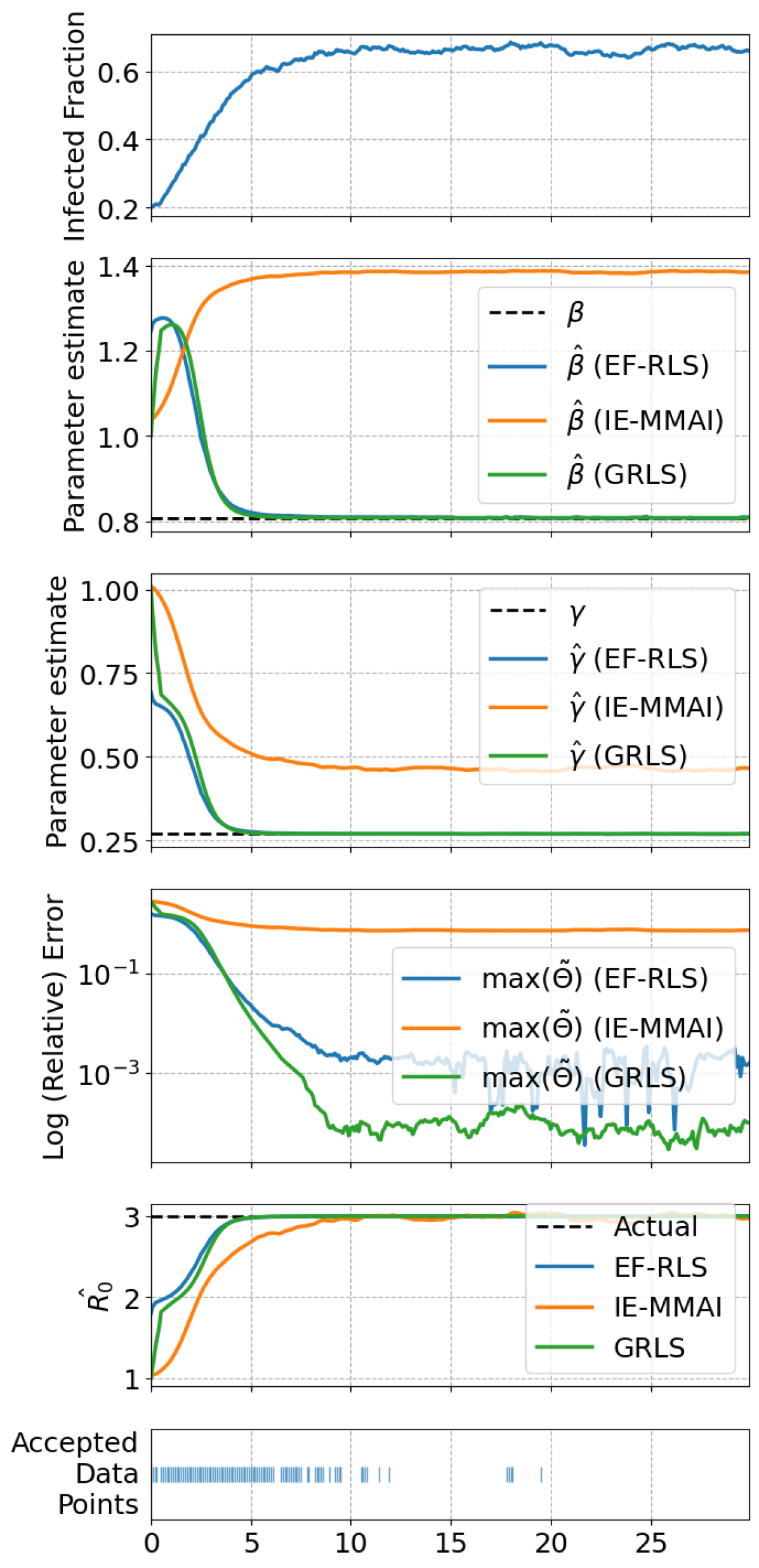
Figure 5: The top panel shows the infected proportion under the SIS model ($\beta=0.8076$, $\gamma=0.2692$). The bottom panel depicts data indices accepted into the greedy excitation set by GRLS. Then, the rest of the panels, arranged from top to bottom, compare the performance of EF-RLS, IE-MMAI, and GRLS: (Top) parameter estimates over time for both noise-free case (left panel) and a noisy simulation (right panel); (Middle) maximum relative error in log scale for parameter estimates over time; (Bottom) reproduction number estimates over time.

IE-MMAI, designed for only LTI systems and as a gradient descent-like, first-order method, is justifiably sensitive to the choice of the initial parameter estimates, and often fails to converge due to the poor practical identifiability of SIS models, as discussed in Example 1. Note that the estimated reproduction numbers still converge to the actual value despite the lack of convergence of the parameter estimates themselves, which is consistent with our discussion of SIS practical identifiability in Section II-C. On the other hand, even in the presence of noise, the parameter estimates converge for both EF-RLS and GRLS.

Data accepted into the GRLS greedy excitation set (8) used to construct the main regressor are diagrammatically depicted in the lowermost block of Fig. 5. A majority of points accepted by the algorithm is in the transient rise of states before the equilibrium is reached. The beginning of the epidemic garners a critical amount of information about the epidemic parameters as would be expected.

Note that while EF-RLS is comparable in performance to GRLS for the noise-free case (left panel of Fig. 5), it becomes increasingly oscillatory upon losing excitation in the noisy case (right panel of Fig. 5). A closer look at the covariance matrix $P_{k}$ for both algorithms reveals a steady increase in the condition number and maximum eigenvalue of $P_{k}$ for EF-RLS, while those of GRLS saturate due to its tendency to avoid picking up non-exciting data points (see Fig. 6). This phenomenon in EF-RLS is observed in both the noise-free and noisy cases and is known in the literature as covariance windup [37], which occurs when a non-unity forgetting factor in EF-RLS causes $P_{k}$ to get closer to a singular matrix upon losing persistence of excitation. The linear increase in the maximum eigenvalue of $P_{k}$ is consistent with past analysis [38]. Upon running the parameter estimation task for longer times, the RLS estimates diverge.

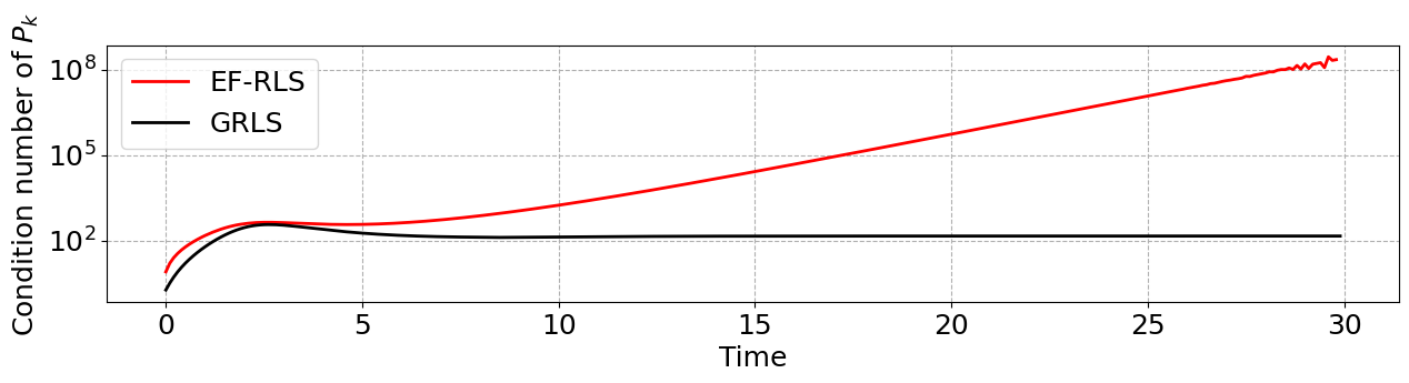
Figure 6: Plot of the condition number of the covariance matrix $P_{k}$ against time for both EF-RLS and GRLS running on data from the noise-free SIS simulation (Fig. 5).

V-B Networked SIR Model

In this section, we aim to investigate the performance of the GRLS algorithm in estimating epidemic parameters under more realistic conditions involving networked structures. Three network topologies are considered in the simulations, which include a fully-connected, a star, and an Erdős-Rényi (ER) [39] network. Fig. 7 shows the three topologies of networked structures we use in this section.

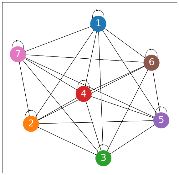
(a) Fully-connected

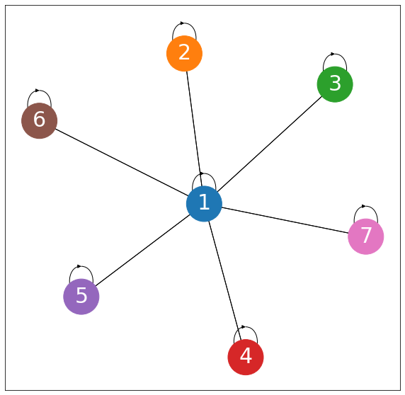
(b) Star

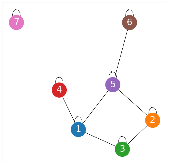
(c) Erdős-Rényi

Figure 7: Fig. 7(a) to 7(c) illustrate the structure of the 7-node networks, where the Erdős-Rényi (ER) network in Fig. 7(c) is generated with $0.50$ edge inclusion probability.

To generalize the $2$-node SIR network, We can rewrite the $2$-node SIR network presented in (21) in a manner akin to (6). Let $n$ be the number of nodes in a network, we choose the regressor $\phi_{k}\in\mathbb{R}^{(2n)\times(n^{2}+n)}$ as follows:

$$\phi_{k}:=\begin{bmatrix}I(t_{k})^{\top}\otimes\text{diag}(1_{n}-I(t_{k})-R(t_{k}))&-\text{diag}(I(t_{k}))\\ 0_{n\times n^{2}}&\text{diag}(I(t_{k}))\end{bmatrix},$$

and the target vector as $\psi_{k}=\begin{bmatrix}\dot{I}(t_{k})^{\top}&\dot{R}(t_{k})^{\top}\end{bmatrix}$, where $I(t)\in[0,1]^{n}$ and $R(t)\in[0,1]^{n}$ represent the infected and recovered proportion of the populations accordingly. The parameter vector $\theta=[\beta,\gamma]^{\top}$ is the concatenated flattened adjacency matrix $\beta=\text{vec}(B)$ (of infection rates between different nodes, not assumed symmetric) and recovery rates vector $\gamma$, such that $\theta\in\mathbb{R}^{n^{2}+n}_{\geq 0}$ is a ($n^{2}+n$)-dimensional vector. Fig. 8 shows the infection levels and their derivatives in the noiseless $7$-node network.

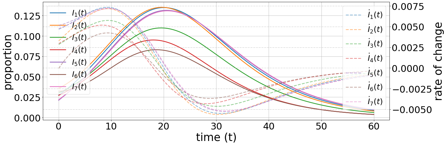
Figure 8: State trajectories of fully-connected networked SIR model without noise.

Before we begin discussing the performance of the system parameters’ estimation, it is helpful to introduce two more notions to help summarize the estimation performance over $50$ parameters. In Example 1, we introduced the basic reproduction number $\mathcal{R}_{0}$ of a single-node SIR/SIS system as the ratio between the infection rate and the recovering rate $\beta/\gamma$. The local basic reproduction number generalizes the notion of basic reproduction number to networked epidemics.

Definition 12 (Local Basic Reproduction Number).

The local basic reproduction number $\mathcal{R}^{0}_{i}\in\mathbb{R}_{\geq 0}$ [40] of node $i$ in a networked SIR system with parameterization $\theta_{\text{SIR}}=(B,\gamma)$ is:

$$\mathcal{R}^{0}_{i}\coloneqq\sum_{j=1}^{n}[\text{diag}(\gamma)^{-1}B]_{ij}.$$ (27)

Definition 13 (Relative Error).

The relative error is defined as $\tilde{\theta}(t)\coloneqq|\frac{\theta_{\text{true}}-\hat{\theta}(t)}{\theta_{\text{true}}+\delta}|$.

We choose $\delta=10^{-2}$ to be the order of magnitude of the smallest positive parameter in the network.

Definition 14 (Relative Error Profile).

Let $p$ be the number of parameters in $\theta$. The relative error profile is defined as the area enclosed by the interval $[\min_{i\in[p]}\{\tilde{\theta}_{i}(t)\},\max_{i\in[p]}\{\tilde{\theta}_{i}(t)\}]$ for all $t_{0}\leq t\leq T$, where $\tilde{\theta}\in\mathbb{R}^{p}$ is a vector with length $p>1$.

Since we have compared the performance of EF-RLS and GRLS with the single-node SIS example, we now proceed to compare the performance of GRLS and the Directional Forgetting Recursive Least Squares (DF-RLS) algorithm [12]. These two algorithms share similar working principles, therefore, the comparison is carried out using the noiseless fully-connected SIR network example shown in Fig. 8.

We show in Fig. 9 that GRLS performs better than DF-RLS in terms of the relative error in the estimation median of $\beta,\gamma,$ and $\mathcal{R}_{0}$.

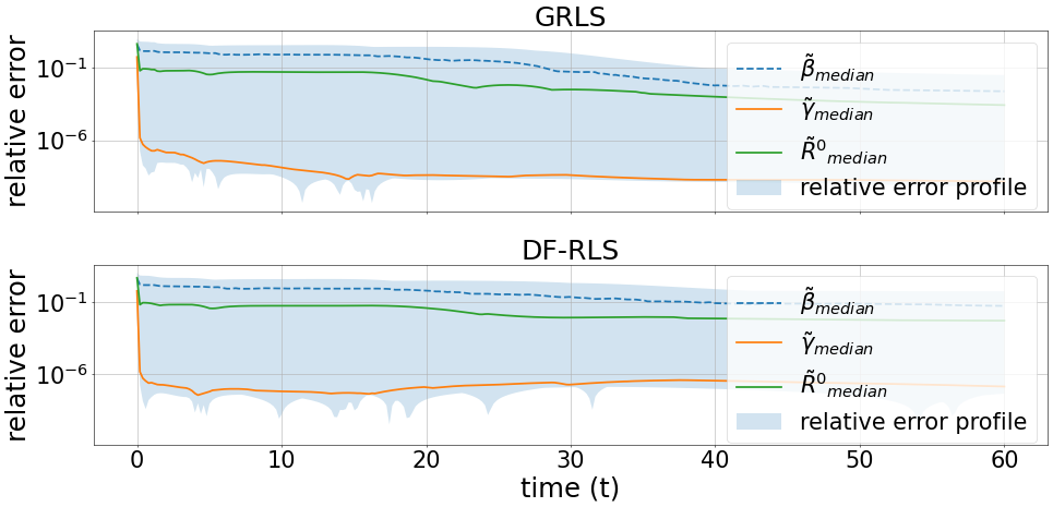
Figure 9: Performance comparison between GRLS and DF-RLS on the noiseless $7$-node fully-connected SIR network.

However, when compared to the single-node SIS parameter estimation in Fig. 5, the relative estimation error increases significantly, by orders of magnitude. The increase is partially due to the curse of dimensionality in the estimation problem. For every node added to the network, there could be $n-1$ extra edges, i.e., the number of system parameters grows quadratically, $\mathcal{O}(n^{2})$, with respect to the number of measured signals, $n$.

In the next example, we allow the process noise to scale with the square root of the state vector $X(t)\coloneqq\begin{bmatrix}I^{\top}(t)&R^{\top}(t)\end{bmatrix}^{\top}$, approximating the arrival of random infection and recovery events under a Poisson distribution[41, pg. 197]. Particularly, we use the following stochastic differential equation of the networked SIR model for simulating a realistic disease outbreak scenario:

$$\mathop{}\!\mathrm{d}X(t)=\mathop{}\!\mathrm{d}\phi(X(t))\theta\mathop{}\!\mathrm{d}t+(\phi(X(t))\text{diag}(\theta))^{\circ 1/2}\mathop{}\!\mathrm{d}W,$$ (28)

where $(\cdot)^{\circ 1/2}$ denotes the element-wise square root, i.e., the Hadamard’s root. Under the same assumption that $\psi_{k}=\begin{bmatrix}\dot{I}(t_{k})^{\top}&\dot{R}(t_{k})^{\top}\end{bmatrix}$ is known, the second term $(\phi(X(t))\text{diag}(\theta))^{\circ 1/2}\mathop{}\!\mathrm{d}W$ in (28) can be effectively treated as known input signal $u(t)$. The synthetic data generated by the Euler–Maruyama method [42] is shown in Fig 10.

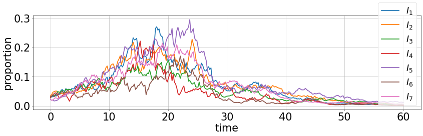
Figure 10: Simulated infection pervalence on the fully-connected network with process noise.

We observe in Fig. 11 that the estimation performance of both the GRLS and DF-RLS algorithms improves significantly with process noise. This improvement is caused by the unconstrained trajectory of $\phi_{k}\top\phi_{k}$ in the simple SIR dynamics. The phenomenon aligns with the intuition we learn from Theorem 1 and Example 1. In practice, the above experiments indicate that process noise might improve identification results with proper techniques of recovering state derivatives [43].

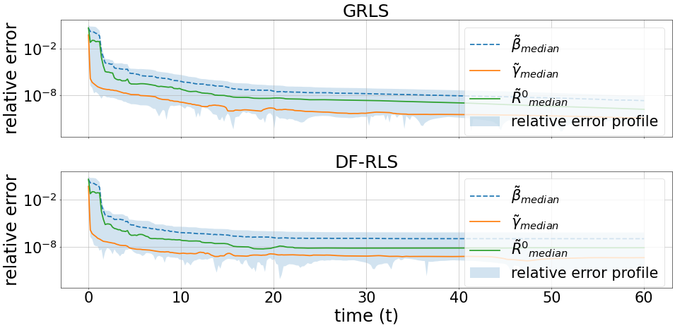
Figure 11: Performance comparison between GRLS and DF-RLS on the $7$-node fully-connected SIR network with known process noise. The estimation with process noise outperforms that of the noiseless example.

To conclude, we examine the identification performance of infection networks under a noiseless scenario. Fig. 12 illustrates the true values and estimation errors of the infection network previously introduced in Fig. 7. We observe that the relative error is highest for the estimation of empty edges, indicating the utility of LASSO regression in contrast to the ridge regression currently used in GRLS, as noted in Corollary 2.2. However, as demonstrated in the comparison between Fig. 9 and 11, the presence of persistently exciting input signals is also crucial for identifying high-dimensional sparse networks.

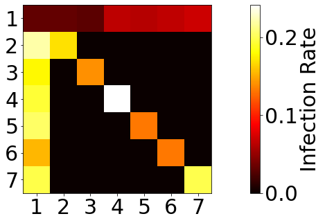
(a) True network (Star)

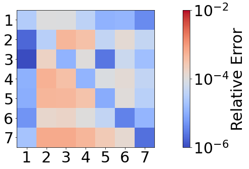
(b) Estimation errors (Star)

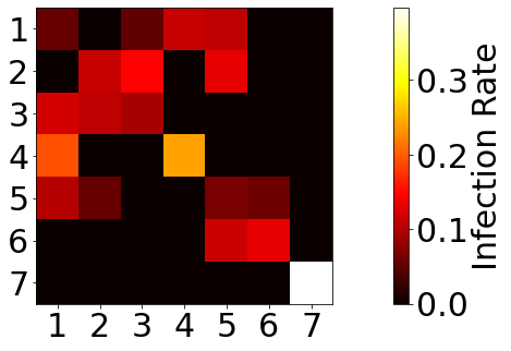
(c) True network (ER)

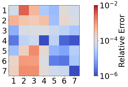
(d) Estimation errors (ER)

Figure 12: Fig. 12(a) and Fig. 12(c) illustrate the matrix form of the star and ER network shown earlier in Fig. 7(b) and Fig. 7(c). Fig. 12(b) and Fig. 12(d) show the relative estimation error of their corresponding rate matrix at time $t=60$.

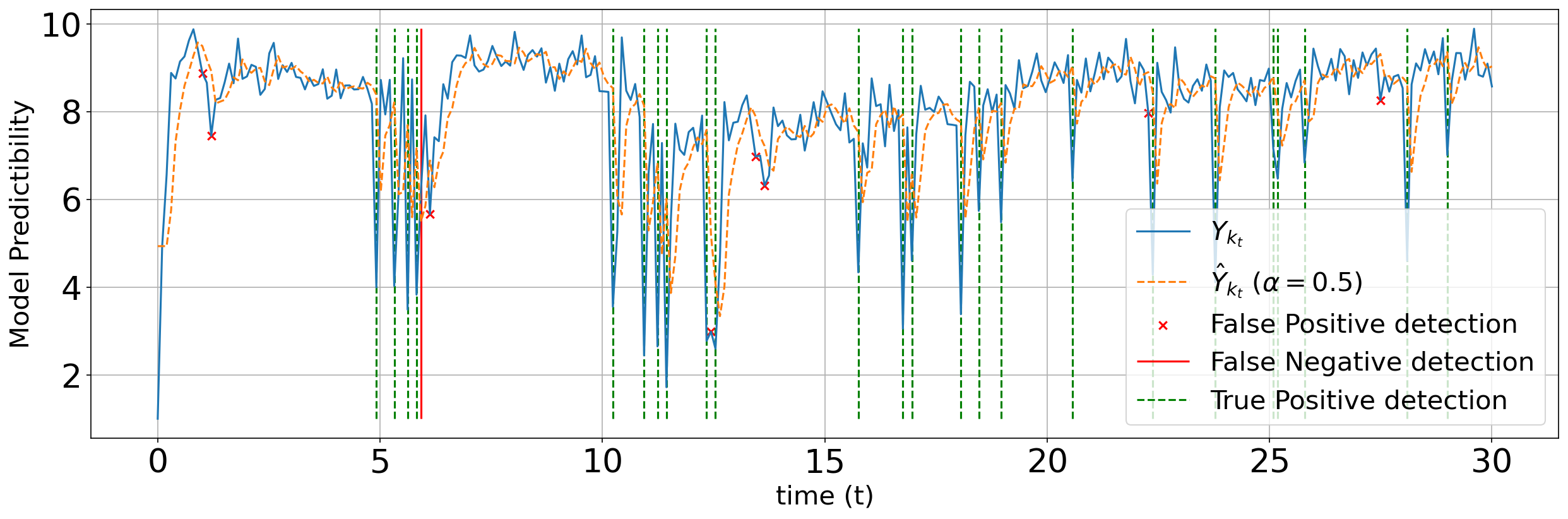
Figure 13: Change point detection performance, significant level is chosen to be $\tau=0.1$ with exponential weight $\alpha=0.5$. The y-axis represents the magnitude of the model predictability $Y_{k}$, with higher values being preferable.

V-C Time-Varying System

In this section, we examine the effectiveness of the change point detection algorithm proposed in Section IV by assessing parameter estimation errors. We start by considering Example 2 with process noise similar to the experimental setup in the previous section. We also added observation noise to the observed signal in the form of (2) with a strength of around one-tenth the value of $\psi_{k}$. Fig. 14 visualizes the infection synthetic data.

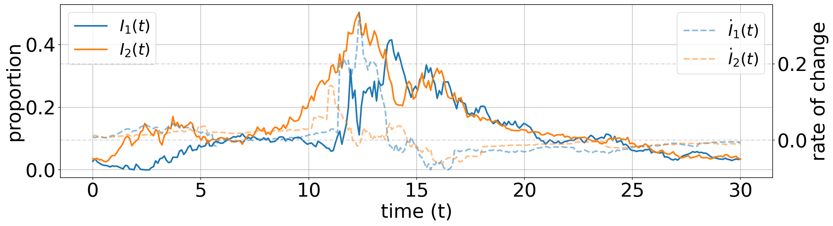
Figure 14: Infection synthetic data of a 2-node SIR network

We attach Algorithm 2 onto an EF-RLS algorithm with an exponentially forgetting rate of $0.98$ through the online estimation scheme, Algorithm 3. The parameter covariance matrix $P_{k}$ is reset to its initial value when a change point is detected by Algorithm 2. Fig. 15 shows that parameter estimation performance is improved significantly through accurate change point detections.

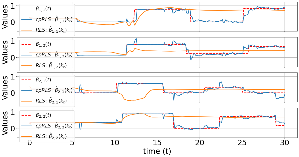
(a) Infection rate

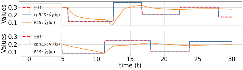
(b) Recovering rate

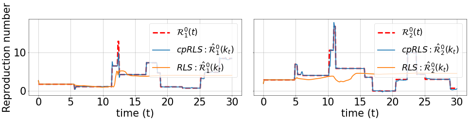
(c) Local basic reproduction number

Figure 15: Parameter tracking performance comparison before and after applying change point detection resetting. Red dotted lines are the true time-varying trajectories, the orange solid lines are the RLS estimates without change-point resetting, and the blue solid lines are the RLS estimates with change-point resetting.

In Figs. 15(a) and 15(b), we observe notable improvement in the tracking performance of the infection and recovery rates. The oscillations in the tracking trajectory in Fig. 15(a) is eliminated in Fig. 15(c) because of the reduced dimension of the tracking parameters, aligning with the observations in Example 1.

Fig. 13 shows the performance of Algorithm 2 in terms of the true positive, false positive, and false negative detection rate. We note that the detection algorithm exhibits commendable efficacy, successfully minimizing false-negatives under a fixed significance level. However, it is worth noting that subsequent detection of true-positive change points relies on the prior successful rejections of false-negative detection occurrences. This dependency arises because any false-negative detection diminishes the accuracy of upstream parameters estimation, leading to a long-term decrease in the magnitude of $Y_{k}$, thus potentially obscuring the impact of future change point arrivals in $Y_{k}$. On the other hand, false-positive detections prematurely reset the estimator’s memory, leading to slow convergence. The above observations suggest that a balance must be struck between true-positive and false-positive rates in the change point detector.

To choose the optimal significant level $\tau$ and exponentially weighted factor $\alpha$ in Algorithm 2, we examine the impact of $\alpha$ on a stochastic signal.

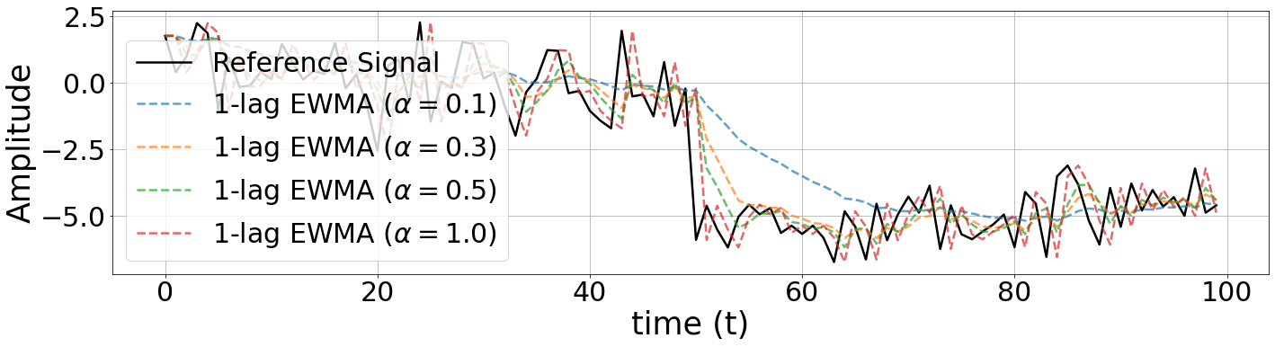
Figure 16: The 1-lagged EWAM acts as a low pass filter on a Gaussian white noise signal with an abrupt downward drift at time $t=50$. Values of $\alpha\in\{0.1,0.3,0.5,1.0\}$ determine the smoothing effect of the EWAM.

In Fig. 16, we can see that the exponential weight $\alpha\in[0,1]$ determines the smoothing intensity of an EWAM. When $\alpha=1$, EWAM corresponds to the most recent update and provides no smoothing effect. As $\alpha$ approaches $0$, EWAM relies solely on its initial value, resulting in maximum smoothing in the cost of prediction power. A high $\alpha$ value entails a higher recall and precision score on the prediction performance, illustrated in Fig. 17.

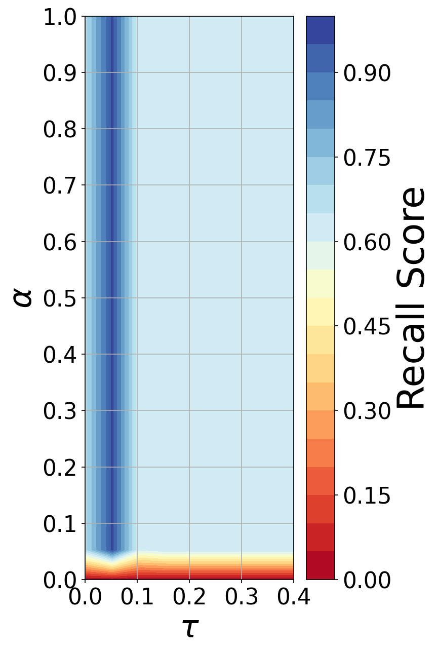
(a) Recall Score

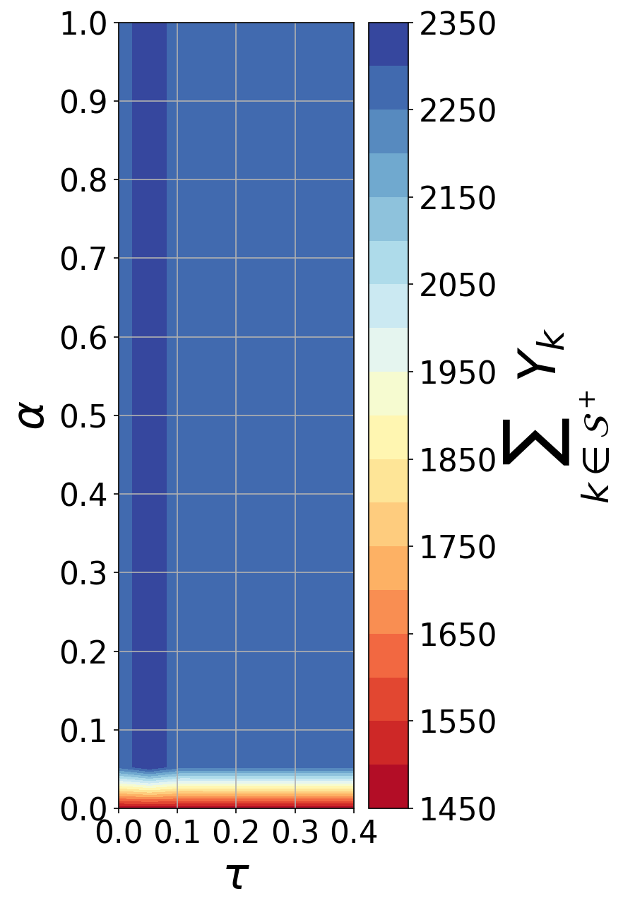
(b) Predictability

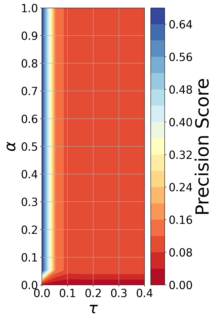
(c) Precision Score

Figure 17: Detection performance metrices with respect to varying significant levels $\tau$, and exponential weights $\alpha$. Fig. 17(a) illustrates the recall score, also known as the true positive rate, in relation to various values of $\tau$ and $\alpha$. Additionally, Figure 17(b) presents the aggregate of model predictability, and it delineates the precision score, which is calculated as $\frac{\text{true positive}}{\text{true positive}+\text{false positive}}$. A high recall and precision score signify good performance of Algorithm 2, whereas a high sum of model predictability indicates a good overall performance of the change-point detection enhanced online estimation process through Algorithm 3.

In Fig. 17, we observe that the surface of the total model predictability, Fig. 17(b), resembles a balance between the recall, Fig. 17(a), and precision score, Fig. 17(c), surfaces. In general, the score surfaces in Fig. 17 remain relatively constant with $\alpha$ until $\alpha<0.1$. This phenomenon occurs due to the loss of EWAM’s predictability when $\alpha=0$.

At times, we realize that the performance of the online estimation algorithm depends on the choice of $\tau$ and $\alpha$. One way to further improve the estimation performance is to look at the Receiver operating characteristic (ROC) curve to pick a threshold and an operating point that maximizes the true-positive rate. Fig. 18 shows the ROC curve of the performance of the change point detection algorithm on RLS and GRLS.

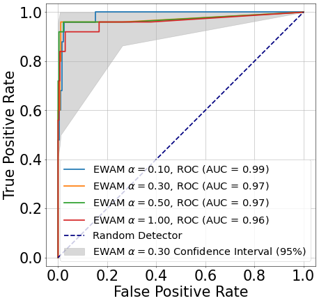
(a) RLS Change point detection ROC curve

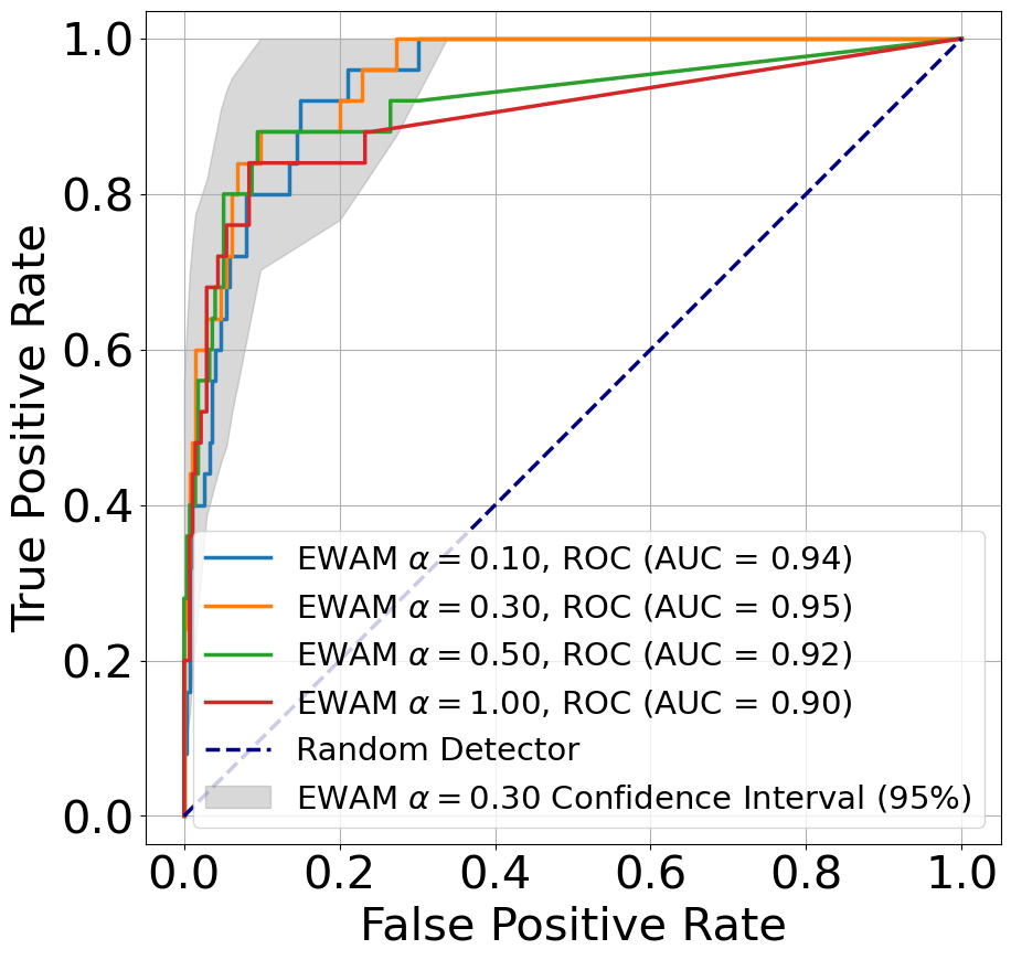
(b) GRLS Change point detection ROC curve

Figure 18: ROC curves that capture the performance of change-point detection for the EF-RLS online estimator (18(a)) and GRLS online estimator (18(b)).

In particular, we can choose $\alpha=0.3$ to maximize the area under the ROC curve. Then, we may pick an operating point that corresponds to a high true positive rate.

VI Conclusion

We have highlighted two problems that plague the application of online parameter estimation tools to nonlinear systems: the lack of persistence of excitation and the practical non-identifiability of epidemic models. We propose a novel algorithm (GRLS) based on recursive least squares and construct an exciting set for the regressor. The GRLS Algorithm has superior performance compared to conventional algorithms and is able to identify epidemic parameters in the networked SIS/SIR model with process and observation noise. Furthermore, we introduce a change-point detection-based memory resetting scheme to aid time-varying parameter tracking. The performance of this parameter tracking scheme is demonstrated in numerical simulation.

Chi Ho Leung is a Ph.D. candidate in the Elmore Family School of Electrical and Computer Engineering at Purdue University studying networked dynamic systems and safety-critical control. He received his M.S. and B.S. in Computer Science from Brigham Young University in 2019 and 2016, respectively. His primary research interests include system identification, online estimation, and automatic control of networks.

Ashish R. Hota is an Assistant Professor in the Department of Electrical Engineering at Indian Institute of Technology (IIT) Kharagpur. He was a postdoctoral researcher at the Automatic Control Laboratory, ETH Zurich in 2018. He received his Ph.D. from Purdue University in 2017, and his B.Tech and M.Tech (dual degree) from Indian Institute of Technology Kharagpur, in 2012, all in Electrical Engineering. He was recognized as a INAE Young Associate in 2023, and received the Outstanding Graduate Researcher Award from the College of Engineering, Purdue University in 2017, and the Institute Silver Medal from IIT Kharagpur in 2012. His research interests are in the areas of (i) game theory and behavioral decision theory, (ii) stochastic optimization, control and learning and (iii) resilience and security of network systems.

Philip E. Paré is the Rita Lane and Norma Fries Assistant Professor in the Elmore Family School of Electrical and Computer Engineering at Purdue University. He received his Ph.D. in Electrical and Computer Engineering (ECE) from the University of Illinois at Urbana-Champaign (UIUC) in 2018, after which he went to KTH Royal Institute of Technology in Stockholm, Sweden to be a Post-Doctoral Scholar. He received his B.S. in Mathematics with University Honors and his M.S. in Computer Science from Brigham Young University in 2012 and 2014, respectively. His research interests include mathematical modeling of dynamic networked systems, e.g. epidemiological, biological, economic systems, infrastructure networks, social networks, etc., and stability analysis, control, and identifiability of such systems.

References

- [1] A. R. Hota, J. Godbole, and P. E. Paré, “A closed-loop framework for inference, prediction, and control of sir epidemics on networks,” IEEE Transactions on Network Science and Engineering, vol. 8, no. 3, pp. 2262–2278, 2021.
- [2] S. A. U. Islam and D. S. Bernstein, “Recursive least squares for real-time implementation [lecture notes],” IEEE Control Systems Magazine, vol. 39, no. 3, pp. 82–85, 2019.
- [3] L. Ljung and T. Glad, “On global identifiability for arbitrary model parametrizations,” Automatica, vol. 30, no. 2, pp. 265–276, 1994.
- [4] P. Ioannou and B. Fidan, Adaptive Control Tutorial. SIAM, 2006.
- [5] K. S. Narendra and A. M. Annaswamy, “Persistent excitation in adaptive systems,” Int. Journal of Control, vol. 45, no. 1, pp. 127–160, 1987.
- [6] N. Cunniffe, F. Hamelin, A. Iggidr, A. Rapaport, and G. Sallet, “Observability, identifiability and epidemiology: A survey,” arXiv preprint arXiv:2011.12202, 2023.
- [7] F.-G. Wieland, A. L. Hauber, M. Rosenblatt, C. Tönsing, and J. Timmer, “On structural and practical identifiability,” Current Opinion in Systems Biology, vol. 25, pp. 60–69, 2021.
- [8] P. Ioannou and J. Sun, “Theory and design of robust direct and indirect adaptive-control schemes,” Int. Journal of Control, vol. 47, no. 3, pp. 775–813, 1988.
- [9] P. A. Ioannou and J. Sun, Robust Adaptive Control. PTR Prentice-Hall Upper Saddle River, NJ, 1996, vol. 1.
- [10] S. K. Jha, S. B. Roy, and S. Bhasin, “Initial excitation-based iterative algorithm for approximate optimal control of completely unknown LTI systems,” IEEE Transactions on Automatic Control, vol. 64, no. 12, pp. 5230–5237, 2019.
- [11] A. Dhar, S. B. Roy, and S. Bhasin, “Initial excitation based discrete-time multi-model adaptive online identification,” European Journal of Control, vol. 68, p. 100672, 2022.
- [12] L. Cao and H. Schwartz, “A directional forgetting algorithm based on the decomposition of the information matrix,” Automatica, vol. 36, no. 11, pp. 1725–1731, 2000.
- [13] B. Lai and D. S. Bernstein, “Generalized forgetting recursive least squares: Stability and robustness guarantees,” IEEE Transactions on Automatic Control, 2024.
- [14] M. E. Salgado, G. C. Goodwin, and R. H. Middleton, “Modified least squares algorithm incorporating exponential resetting and forgetting,” Int. Journal of Control, vol. 47, no. 2, pp. 477–491, 1988.
- [15] P. Fearnhead, “Exact and efficient bayesian inference for multiple changepoint problems,” Statistics and Computing, vol. 16, pp. 203–213, 2006.
- [16] N. Mohseni and D. S. Bernstein, “Recursive least squares with variable-rate forgetting based on the f-test,” in Proc. 2022 American Control Conference (ACC). IEEE, 2022, pp. 3937–3942.
- [17] J. S. Hunter, “The exponentially weighted moving average,” Journal of quality technology, vol. 18, no. 4, pp. 203–210, 1986.
- [18] R. V. Hogg, E. A. Tanis, and D. L. Zimmerman, Probability and Statistical Inference. Macmillan New York, 1977, vol. 993.
- [19] B. Prasse and P. Van Mieghem, “Predicting network dynamics without requiring the knowledge of the interaction graph,” Proceedings of the National Academy of Sciences, vol. 119, no. 44, p. e2205517119, 2022.
- [20] W. O. Kermack, A. G. McKendrick, and G. T. Walker, “A contribution to the mathematical theory of epidemics,” Proceedings of the Royal Society of London. Series A, Containing Papers of a Mathematical and Physical Character, vol. 115, no. 772, pp. 700–721, 1927.
- [21] G. Giordano, F. Blanchini, R. Bruno, P. Colaneri, A. Di Filippo, A. Di Matteo, and M. Colaneri, “Modelling the COVID-19 epidemic and implementation of population-wide interventions in Italy,” Nature Medicine, vol. 26, no. 6, pp. 855–860, 2020.
- [22] C. H. Leung, W. E. Retnaraj, A. R. Hota, and P. E. Paré, “Adaptive identification of sis models,” in Proc. 2023 Ninth Indian Control Conference (ICC). IEEE, 2023, pp. 168–173.
- [23] R. A. Johnson, D. W. Wichern et al., Applied Multivariate Statistical Analysis. Prentice Hall Upper Saddle River, NJ, 2002.
- [24] R. Bellman and K. J. Åström, “On structural identifiability,” Mathematical biosciences, vol. 7, no. 3-4, pp. 329–339, 1970.
- [25] D. M. Hamby, “A review of techniques for parameter sensitivity analysis of environmental models,” Environmental monitoring and assessment, vol. 32, pp. 135–154, 1994.
- [26] E. R. Kolchin, Differential algebra & algebraic groups. Academic press, 1973.
- [27] E. Panteley, A. Loria, and A. Teel, “Relaxed persistency of excitation for uniform asymptotic stability,” IEEE Transactions on Automatic Control, vol. 46, no. 12, pp. 1874–1886, 2001.
- [28] W. Rudin et al., Principles of Mathematical Analysis. McGraw-hill New York, 1964, vol. 3.
- [29] R. A. Horn and C. R. Johnson, Matrix Analysis. Cambridge university press, 2012.
- [30] G. Bengtsson, “Output regulation and internal models—a frequency domain approach,” Automatica, vol. 13, no. 4, pp. 333–345, 1977.
- [31] P. E. Paré, C. L. Beck, and T. Başar, “Modeling, estimation, and analysis of epidemics over networks: An overview,” Annual Reviews in Control, vol. 50, pp. 345–360, 2020.
- [32] K. S. Narendra and A. M. Annaswamy, Stable Adaptive Systems. Courier Corporation, 2012.
- [33] A. Goel, A. L. Bruce, and D. S. Bernstein, “Recursive least squares with variable-direction forgetting: Compensating for the loss of persistency [lecture notes],” IEEE Control Systems Magazine, vol. 40, no. 4, pp. 80–102, 2020.
- [34] J. Benesty and T. Gansler, “A recursive estimation of the condition number in the rls algorithm [adaptive signal processing applications],” in Proceedings.(ICASSP’05). IEEE International Conference on Acoustics, Speech, and Signal Processing, 2005., vol. 4. IEEE, 2005, pp. iv–25.
- [35] D. S. Bernstein, Matrix Mathematics. Princeton University Press, 2009.
- [36] S. S. Wilks, “The large-sample distribution of the likelihood ratio for testing composite hypotheses,” The Annals of Mathematical Statistics, vol. 9, no. 1, pp. 60–62, 1938.
- [37] T. Fortescue, L. S. Kershenbaum, and B. E. Ydstie, “Implementation of self-tuning regulators with variable forgetting factors,” Automatica, vol. 17, no. 6, pp. 831–835, 1981.
- [38] L. Cao and H. Schwartz, “The Kalman filter based recursive algorithm: Windup and its avoidance,” in Proc. American Control Conference, 2001, pp. 3606–3611.
- [39] P. Erdős and A. Rényi, “On random graphs i.” Publ. Math. Debrecen, vol. 6, no. 290-297, p. 18, 1959.
- [40] B. She, P. E. Paré, and M. Hale, “Distributed reproduction numbers of networked epidemics,” in Proc. American Control Conference, 2023, arXiv preprint arXiv:2301.07837.
- [41] M. J. Keeling, Modeling Infectious Diseases in Humans and Animals. Princeton University Press, 2008.
- [42] G. Maruyama, “Continuous markov processes and stochastic equations,” Rendiconti del Circolo Matematico di Palermo, vol. 4, pp. 48–90, 1955.
- [43] R. Chartrand, “Numerical differentiation of noisy, nonsmooth data,” International Scholarly Research Notices, vol. 2011, 2011.