A Near-Optimal Category Information Sampling in RFID Systems

Abstract

In many RFID-enabled applications, objects are classified into different categories, and the information associated with each object’s category (called category information) is written into the attached tag, allowing the reader to access it later. The category information sampling in such RFID systems, which is to randomly choose (sample) a few tags from each category and collect their category information, is fundamental for providing real-time monitoring and analysis in RFID. However, to the best of our knowledge, two technical challenges, i.e., how to guarantee a minimized execution time and reduce collection failure caused by missing tags, remain unsolved for this problem. In this paper, we address these two limitations by considering how to use the shortest possible time to sample a different number of random tags from each category and collect their category information sequentially in small batches. In particular, we first obtain a lower bound on the execution time of any protocol that can solve this problem. Then, we present a near-OPTimal Category information sampling protocol (OPT-C) that solves the problem with an execution time close to the lower bound. Finally, extensive simulation results demonstrate the superiority of OPT-C over existing protocols, while real-world experiments validate the practicality of OPT-C.

1 Introduction

Radio frequency identification (RFID) technology, with many shining advantages such as non-line-of-sight detection and low manufacturing costs, has been used in many applications, ranging from object tracking and positioning [1, 2] to supply chain control and scheduling [3, 4, 5]. Typically, these applications track objects belonging to various categories, such as types of drugs in a pharmacy, topics of books in a library, or brands of food in a supermarket. Whenever a tag is attached to one of these objects, information related to the category of the object (called category information) can be written to this tag to make it readily available to RFID readers in an offline manner (without consulting a remote reference database) [6, 7]. Such category information on tags can be either static data (e.g., the brand of a garment) or dynamic data (e.g., continuous sensory readings from a tag’s integrated sensor) [8, 9, 10].

In RFID systems for such applications, tags are systematically classified, with all tags within the same category sharing identical category information. In an ideal scenario, assuming all tags are present and functioning correctly in an interference-free environment, querying a single random tag per category would provide a comprehensive view of the category information. However, practical realities necessitate a departure from this ideal. Overreliance on a single random tag per category is often insufficient, primarily due to the potential absence of the selected tag. Missing tags may result from various factors, such as their location beyond the reader’s detection range, signal interference, or hardware malfunctions [7, 11]. For instance, a tag may become unresponsive when obstructed by signal-shielding materials like metal surfaces or when its backscattered signal lacks sufficient power or becomes corrupted, rendering it undetectable [12, 13].

Therefore, in this paper, we consider the practical RFID system with missing tags and study the Category Information Sampling Problem (the CIS problem), which is to use the shortest possible time to randomly choose a user-specific number of tags from each category and read them. Here, we afford users the flexibility to specify in advance how many tags they would like to randomly choose from each category, which can be used to mitigate collection failures caused by missing tags or for other practical objectives (e.g., data consistency verification and the estimation of category-specific statistics). This problem holds significant relevance to real-time monitoring of tagged objects and the on-the-fly analysis of their category data within RFID systems. For instance, consider a supermarket that organizes food products based on their expiration dates, with these dates recorded on attached tags as category information. Due to signal interference or hardware issues, certain tags might be missing. In such cases, swift sampling of expiration dates from randomly selected tags within each category enables real-time tracking of food quality. Similarly, in a bustling logistics center, shipping items are classified by their destination addresses, written on attached tags as category information. Given the rapid movement of these items, some tags may be missed if they exit the reader’s detection area. To ensure timely collection and analysis of shipping addresses, it’s imperative to sample multiple tag addresses from each category, rather than relying on just one tag. Numerous real-world situations present similar contexts where multiple tags convey identical or similar data, necessitating immediate tracking and analysis [6, 7]. In addition, it is essential to note that various practical RFID scenarios may prompt readers to read multiple tags randomly selected from each category, going beyond the core objective of addressing missing tags. These supplementary purposes encompass tasks such as verifying data consistency and estimating category-specific statistics [7, 9, 14].

In essence, the investigation of the CIS problem within RFID systems holds the potential to significantly enhance the efficiency and reliability of RFID systems, catering to a wide array of critical applications. This empowers users with the capability to fine-tune their tag selection strategies to address challenges like missing tags and extend their applications to encompass broader objectives such as data validation and statistical estimation.

1.1 Prior Art and Limitations

Numerous protocols exist for extracting data from a tag subset, denoted as $P$, in RFID systems [9, 10, 15, 16, 17, 18]. These protocols often employ Bloom filters or their variants to distinguish the desired subset $P$ from the entire tag population and subsequently retrieve information from the tags within $P$. For example, ETOP [15] employs multiple Bloom filters to filter out non-target tags within the subset $P$. Similarly, TIC [10] reads a subset $P$ of tags in multi-reader RFID systems, using a single-hash Bloom filter to eliminate irrelevant tags. However, it is important to note that transmitting Bloom filters and addressing hash collisions can still be time-consuming [19].

To the best of our knowledge, for RFID systems with multiple categories of tags, TPS [6] and ACS [7] are the only two works that collect category information from randomly sampled tags. TPS [6] capitalizes on the fact that all tags of the same category have a common category-ID (indicating which category they belong to) to collect category information from one random tag of each category. Specifically, it hashes all tags into slots of a communication frame based on their category-ID and finds those homogeneous slots that are occupied only by tags of the same category. Since the category information of the tags in the homogeneous slots is the same, it selects and reads one tag in each homogeneous slot. However, TPS takes a long time to execute because it transmits many useless empty slots in each frame. ACS [7] follows TPS, but uses arithmetic coding to compress each communication frame to reduce transmission costs. With ACS, the reader compresses a frame into a binary fraction and sends it to all tags; each tag decompresses the fraction to recover the frame. Even so, the execution time of ACS is still long and unsatisfactory since it compresses many useless empty slots in each frame; and the arithmetic encoding is too complex for ordinary RFID tags to support [20].

Ultimately, existing tag sampling protocols suffer from three primary drawbacks:

1. Absence of Execution Time Benchmark: There is no known lower bound on the execution time of any protocol that can solve the CIS problem. Establishing such lower bound is crucial for measuring protocol performance and determining the potential for improvement.

2. High Execution Times: Current sampling protocols exhibit unacceptably high execution times, failing to meet the lower bound. This is particularly problematic for RFID systems, where efficient category information retrieval from numerous tags is vital for real-time monitoring and analysis. Achieving execution times close to the lower bound enables us to predict the minimum time required for specific sampling tasks and allocate precise time windows to optimize system efficiency.

3. Neglect of Missing Tags: Existing protocols primarily focus on randomly selecting one tag from each category. However, this approach often falls short because some tags in each category may be missing due to factors like moving out of the reader’s range, hardware issues, or signal interference. Consequently, it is more practical to sample a user-specified number of tags from each category, a reasonable requirement that the current protocol inadequately address.

In addition, it’s worth noting that several concurrent tag identification protocols [21, 22, 23, 24] have been developed to recover signals from collided tags using parallel decoding techniques and specialized equipment like USRP. For example, the Buzz protocol [21] is a pioneering approach that effectively coordinates tags to measure their channel coefficients and reconstructs the transmitted signal of each tag. In recent [24], a novel protocol named CIRF is proposed to address challenges posed by noisy channels, which can introduce errors when recovering tag signals. CIRF leverages multiple antennas to enhance robustness against noise and uses block sparsity-based optimization techniques to restore signals from collided tags. However, these advanced protocols excel in identifying all tags at the physical layer and primarily focus on comprehensive tag identification rather than random sampling from a subset of tags.

1.2 Technical Challenges and Contributions

This paper addresses the Category Information Sampling Problem within the context of RFID systems, where the tag population is categorized into $K$ distinct subsets denoted as $P_{1},P_{2},...,P_{K}$. The primary objective is to randomly select a user-defined number of tags, denoted as $c_{k}$, from each category $P_{k}$ and assign them unique reporting orders for sequential reading while minimizing the execution time. The parameter $c_{k}$, called the reliability number, serves as a user-adjustable parameter aimed at mitigating collection failures caused by missing tags. Additionally, it’s worth mentioning that the user-adjustable parameter, $c_{k}$, holds a broader spectrum of applications beyond addressing missing tag issues, as it could be employed for tasks such as category statistics estimation and security enhancement [7, 9, 10, 11, 14].

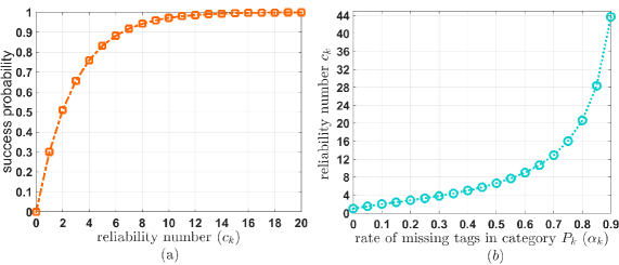
Figure 1: Ensuring High Success Probability with a Small Reliability Number. Note: (a) The success probability demonstrates rapid growth as the reliability number $c_{k}$ increases, even when a substantial portion ($70\%$) of tags in $P_{k}$ are missing ($\alpha_{k}=0.7$). (b) This graph illustrates the reliability number $c_{k}$ that can secure a high success probability of 0.99, as $\alpha_{k}$ varies from $0.05$ to $0.9$.

Please note that the significance of selecting a suitable value for $c_{k}$ becomes apparent when considering the issue of missing tags. Sampling a single tag from category $P_{k}$ carries the risk of encountering missing tags. Hence, users can set $c_{k}$ to substantially increase the success probability, which represents the likelihood that at least one of the $c_{k}$ randomly selected tags is not missing, as illustrated in Fig. 1.

Addressing the studied problem entails overcoming two major challenges to achieve a near-optimal solution:

Challenge 1: Deriving a Non-Trivial Lower Bound on Execution Time

Previous research on the CIS problem has proposed protocols for addressing it [6, 7]. However, these works have not ventured into the domain of lower bound derivation, which serves as a fundamental benchmark for assessing the performance of these protocols. Deriving this lower bound necessitates addressing two technical problems:
(p-1) Analyzing Required Information for Random Tag Selection and Reporting Orders Assignment: This analysis entails dissecting the information that the reader must transmit to achieve the random selection of a user-defined number of tags from each category and assign unique reporting orders to each selected tag. It aims to identify the essential data within the reader’s broadcasted message and how it contributes to solving the CIS problem at the tag side.
(p-2) Determining Minimum Bits for Information Representation: This step involves ascertaining the minimum number of bits to represent the information needed for (p-1), considering all possible tag populations and categories. It seeks to maximize bit utilization while accommodating constraints arising from the problem’s inherent nature and practical considerations within RFID systems.

It’s worth noting that previous research in this field has not provided solutions to these intricate challenges. Given the practical significance of the CIS problem, we are motivated to tackle these problems. Unlike conventional RFID research, which relies on established lower bounds from communication complexity theory [11, 32, 33], our work is uniquely demanding, as we must develop lower bounds from scratch due to the absence of pre-existing references.

Challenge 2: Achieving Near-Optimal Execution Time in Solving the Problem

Prior studies [6, 7] have proposed protocols for randomly selecting a single tag from category $P_{k}$. However, these protocols adopt the global hashing approach, which slot all tags in the entire population into different communication slots but exploit only the homogeneous slots (a small fraction of all slots) to select tags and read their category information. This method inevitably leads to a high number of collisions and empty slots due to hash collisions, resulting in significant transmission overhead. Consequently, these protocols fall short of approaching the derived lower bound on execution time.

In contrast, our proposed two-stage protocol, OPT-C, departs from this global hashing approach. OPT-C comprises OPT-C1 and OPT-C2. OPT-C1 rapidly selects slightly more than $c_{k}$ tags from each category $P_{k}$, while OPT-C2 refines the selection process to choose exactly $c_{k}$ tags and assign unique reporting orders. These stages introduce two technical problems:
(p-3) Designing a Bernoulli Trial for OPT-C1: OPT-C1 necessitates the design of a Bernoulli trial capable of swiftly selecting slightly more than $c_{k}$ tags randomly from category $P_{k}$. Each tag simultaneously receives a threshold value $\bm{\tau}$ from the reader and uses its local hash value to determine its selection status. This process entails performing a Bernoulli trial in parallel on all tags within each category. However, the number of tags selected by a Bernoulli trial is a random variable, not a fixed number. Consequently, this aspect poses a challenge, demanding the careful design of a Bernoulli trial with an appropriate threshold value of $\bm{\tau}$. This ensures that the probability of selecting slightly more than $c_{k}$ tags is sufficiently high while maintaining almost negligible execution time costs. Please note that, as the Bernoulli trial operates in parallel on all tags, the communication overhead of OPT-C1, involving only the transmission of a hash seed and a threshold value, remains minimal.
(p-4) Designing a Refined Sampling Protocol for OPT-C2: OPT-C2, tasked with the selection of exactly $c_{k}$ tags and their assignment of unique reporting orders, presents an intricate challenge. It requires ensuring that OPT-C2 operates with an execution time close to the derived lower bound. Achieving this requires a lot of time and efforts to get a near optimal answer, as detailed in subsequent sections.

In summary, this paper contributes the following:
$\bullet$ We obtain a lower bound on the execution time for the CIS problem.
$\bullet$ We propose a near-OPTimal Category-information sampling protocol (OPT-C) that solves the problem with an execution time close to the lower bound.
$\bullet$ We conduct real-world experiments to verify the practicability and validity of OPT-C; we have also run extensive simulations comparing OPT-C with state-of-the-art protocols, and the results clearly show that OPT-C is much faster than existing protocols and is close to the lower bound.
$\bullet$ We implement the OPT-C protocol on commercial off-the-shelf (COTS) devices and test it in a real RFID system alongside other state-of-the-art C1G2-compatible tag sampling protocols. The experimental results indicate that the actual implementation of OPT-L (denoted by $\text{OPT-C}_{\mathbf{IMPL}}$) achieves an average reduction in execution time of $37\%$ compared to other protocols.

The subsequent sections of this paper are organized as follows: Section 2 defines the CIS problem and presents the lower bound on execution time. Section 3 delves into the OPT-C protocol and establishes its near-optimality. Section 4 focuses on the real-world implementation of OPT-C in RFID systems. Section 5 presents the simulation results for OPT-C, showcasing its superior performance. In Section 6, we present experimental findings that highlight the practicality and efficiency of OPT-C’s implementation. Finally, Section 7 offers concluding remarks.

2 Lower bound on execution time

This section first defines the Category Information Sampling Problem and then obtains a lower bound on the execution time required by any protocol that can solve the problem. To arrive at this lower bound, we employ encoding arguments, a technique commonly used to analyze space constraints in data structures [34], along with convex optimization techniques [35]. Our analysis primarily focuses on the communication exchanges between the reader and the tags when dealing with different input scenarios. The ultimate goal is to determine the minimum number of communication messages needed to effectively handle all possible instances.

2.1 System model and problem formulation

We focus on a typical RFID system [7, 11, 29, 30, 31, 36] that consists of a reader $R$ and a population $S$ of $N$ tags. Reader $R$ connects to the backend server via a high-speed link to obtain computing and storage resources, but it can only communicate with tags via a low-speed wireless link. A tag in population $S$ has an ID ($96$-bit ID), which is a unique identifier for both itself and the associated physical object, and a category-ID, which indicates which category it belongs to. Tags with the same category-ID carry the same category information. In short, each tag $t\in S$ has a unique ID (also represented by $t$), a category-ID $t^{\textbf{G}}$, and a piece of category information. According to category-IDs, population $S$ is partitioned into $K$ categories ($K$ disjoint subsets): $P_{1},P_{2},...,P_{K}$, where each category $P_{k}$ consists of tags having category-ID $k$, $k\in\{1,2,...,K\}$. Moreover, let $n_{k}$ denote the size of category $P_{k}$, i.e., $n_{k}$ is the number of tags in $P_{k}$, and let $c_{k}$ denote the reliability number pre-specified by the user for category $P_{k}$, i.e., $c_{k}$ is the number of tags that should be randomly selected from category $P_{k}$. Tab. I lists the symbols used in this paper.

Initially, reader $R$ knows the IDs and category-IDs of all tags in $S$, but $R$ has no knowledge of their category information or which of them are currently missing. Reader $R$ wishes to randomly select $c_{k}$ tags from each category $P_{k}$, $k\in\{1,2,...,K\}$, and collect their category information.

TABLE I: Symbol Definitions

$U$	The set of all possible tags with ID values ranging from $0$ to $\Upsilon-1$, where $\Upsilon=2^{96}$.
$S$	A tag population of $N$ tags from $U$.
$t$	A tag in $S$ which has a unique $96$-bit ID (also denoted by $t$), a category-ID $t^{\textbf{G}}\in\{1,2,...,K\}$, and a piece of category information.
$K$	The number of categories in $S$.
$P_{k}$	The $k$-th category of tags in $S$ ($P_{k}\subset S$) in which all tags share the same category-ID $k$ and are written with the same category information related to $P_{k}$.
$c_{k}$	The reliability number used for category $P_{k}$, representing the user wants to select $c_{k}$ tags randomly from $P_{k}$.
$n_{k}$	The size of category $P_{k}$, i.e., the number of tags in $P_{k}$.
$\mathbb{P}$	A partition over the universe $U$ according to the written category information on tags, and $\mathbb{P}=\{P_{1},P_{2},...,P_{K},U-S\}$ $\forall i\neq j$, $P_{i}\cap P_{j}=\emptyset$, $\bigcup\nolimits_{k=1}^{K}{{P_{{\color[rgb]{0,0,0}k}}}}=S$. Note that $U-S$ is the remainder set containing all tags that do not appear in $S$.
$R$	A reader, who initially knows only the ID and category-ID of each tag $t$ in $S$ and wants to select a few random tags from each category $P_{k}$ and assign them unique reporting orders.

Definition 2.1

Given an RFID system as described above, the Category Information Sampling Problem (the CIS problem) is to design a protocol $A$ between the reader $R$ and the tags such that the following two objectives are achieved on each category $P_{k}$, $k\in\{1,2,\cdots,K\}$.
(I) Every subset of $c_{k}$ tags from $P_{k}$ has the same probability $1/(_{\,c_{k}}^{n_{k}})$ of being chosen to become the sampled subset $T_{k}$;
(II) Each tag in the sampled subset $T_{k}$ is informed of a unique integer from $\{1,2,\cdots,c_{k}\}$, known as the reporting order of the tag.

Note: the second objective (II) is necessary for collecting category information from the $c_{k}$ tags in $T_{k}$ because reader $R$ can only read the data on the tags sequentially one by one. Fig. 2 provides an example of this problem.

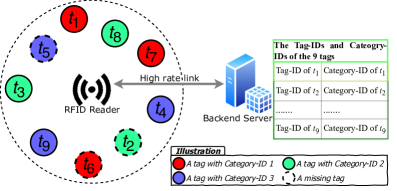
Figure 2: An example of the Category Information Sampling Problem in an RFID system with missing tags. Suppose $c_{1}=1$, $c_{2}=1$, $c_{3}=2$. Then the Category Information Sampling Problem requires the reader to randomly select one tag from $P_{1}$ and read it, randomly select one tag from $P_{2}$ and read it, and randomly select two tags from $P_{3}$ and read them. Note that the three tags: $t_{2},t_{5},t_{6}$ are missing, but the reader does not know this fact.

2.2 A lower bound on execution time

The following theorem establishes a lower bound on the communication time between the reader $R$ and tags, and then obtains a lower bound on the execution time, ${\rm{T}_{{\rm{lb}}}}$.

First, we present some notations needed in the proof. Let $U$ represent the universe of all possible tags with ID values ranging from $0$ up to $\Upsilon-1$, where $\Upsilon=2^{96}$; As each tag owns a unique ID, $U$ also represents the universe of all $2^{96}$ possible IDs. Let us call $U-S$ (i.e., $U-\bigcup\nolimits_{k=1}^{K}{P_{k}}$) the remainder set, and consider the set-family $\mathbb{P}=\{P_{1},P_{2},\cdots,P_{K},U-S\}$. Given a tag population size $N$ and $K$ category sizes: $n_{1},n_{2},\cdots,n_{K}$, the universe $U$ can be arbitrarily partitioned into category $P_{1}$ of $n_{1}$ tags, category $P_{2}$ of $n_{2}$ tags, $\cdots$, category $P_{K}$ of $n_{K}$ tags, and the remainder set of $\Upsilon-N$ tags, denoted by $(_{n_{1},n_{2},\cdots,n_{K},\Upsilon-N}^{\quad\;\;\;\;\;\;\;\;\Upsilon})$, i.e., partition $\mathbb{P}$ has $(_{n_{1},n_{2},\cdots,n_{K},\Upsilon-N}^{\quad\;\;\;\;\;\;\;\;\Upsilon})$ different possibilities. In the following, we use $(_{n_{1},n_{2},\cdots,n_{K}}^{\quad\;\;\;\;\Upsilon})$ to represent the number of possible partitions over the universe $U$, because $\sum\nolimits_{k=1}^{K}n_{k}=N$ and $(_{n_{1},n_{2},\cdots,n_{K},\Upsilon-N}^{\quad\;\;\;\;\;\;\;\;\Upsilon})=(_{n_{1},n_{2},\cdots,n_{K}}^{\quad\;\;\;\;\Upsilon})$.

When exploring the lower bound of protocol execution time, we take the communication time between reader $R$ and tags as the primary determinant, since $R$ has a high-speed connection to the backend server but communicates with tags via a low-speed link slowly [6, 11, 15, 36]. In addition, we omit the computation time of reader $R$ since the backend server can provide computation assistance very quickly, and our lower bound is still valid even with computation time included.

Theorem 2.2

Any protocol $A$ that solves the Category Information Sampling Problem described in Definition 2.1, must satisfy the following two inequalities

$$|A|\geq\Gamma=\sum\nolimits_{k=1}^{K}{\log_{2}(e)c_{\color[rgb]{0,0,0}k}},$$ (1)

$${\rm{T}_{{\rm{lb}}}}\geq{{\rm{T}}_{{\rm{96}}}}\times\Gamma/96,$$ (2)

where ${\rm{T}}_{{\rm{96}}}$ is the time cost of transmitting $96$ bits between reader $R$ and tags, $|A|$ represents the number of bits communicated between reader $R$ and tags during $A$’s execution, and ${\rm{T}_{{\rm{lb}}}}$ represents the lower bound of $A$’s execution time.

Proof:

Let M denote the complete set of communicated messages between reader $R$ and tags during $A$’s execution. Then, $|A|$ equals the number of bits contained in M. Clearly, if protocol $A$ can solve the CIS problem with $K$ given category sizes: $n_{1},n_{2},...,n_{K}$, it must take care of all the $(_{n_{1},n_{2},\cdots,n_{K}}^{\quad\;\;\;\;\Upsilon})$ different partitions. Therefore, in order to obtain the required lower bound, we will study how many bits are needed for message M to handle all these partitions. Below is a roadmap of our proof.

• First, we model the decision process on each tag $t\in S$ and explain how message M helps $t$ to decide whether it is sampled or not, and if so, what its reporting order is.

• Second, we analyze how a specific value $v$ of message M can help solve the CIS problem and how many different partitions it can handle;

• Third, since there are $(_{n_{1},n_{2},..,n_{K}}^{\quad\;\;\;\;\Upsilon})$ different partitions to be handled when solving this problem, we can obtain the lower bound on M by analyzing how many different values the message M must have to handle all these partitions.

As a starting point, we model each tag’s decision process and describe how each tag changes its state after protocol A’s execution (i.e., after receiving message M). In this way, we lay the foundation for our proof. Without loss of generality, we denote the internal decision process on each tag $t\in S$ by a function $F()$. Initially, each tag $t\in S$ is in the same state, which means it doesn’t know whether it needs to report or not, and if so, what its report number is. After receiving message M, tag $t$ takes a category-ID $k$ ($k\in\{1,2,...,K\}$), M, and its ID (also represented by $t$) as the three input parameters to function $F()$, and then computes $F(k,\textit{M},t)$ to decide whether it will be a sampled tag in category $P_{k}$ (the $k$-th category), and if so, what its reporting order is. More specifically, without sacrificing generality, we assume the following decision rules on tag $t$.

• If $F(k,\textit{M},t)=0$, tag $t$ identifies itself as a non-sampled tag in category $P_{k}$.

• If $F(k,\textit{M},t)=i\in\{1,2,\cdots,c_{k}\}$, tag $t$ identifies itself as a sampled tag in category $P_{k}$ and takes $i$ as its reporting order.

Clearly, message M is the parameter that determines the behavior of the $K$ functions: $F(k,\textit{M},\bullet)$, $k=1,2,...,K$. That is, a specific value $v$ of M (M is used as the second parameter of function $F()$) uniquely determines how function $F(k,\textit{M},\bullet)$ maps the $\Upsilon=2^{96}$ tags from $U$ into the range $\{0,1,2,...,c_{k}\}$.

Next, we analyze the number of different partitions that a specific value $v$ can handle. Let $S^{v}_{k,i}$ represent the set consisting of those tags from $U$ that have function $F(k,v,\bullet)$ equal to $i$, or namely the following:

$$S^{v}_{k,i}=\{t|t\in U\,\text{and}\,F(k,v,t)=i\},$$

$$\quad\quad\quad\quad\quad\quad k\in\{1,2,...,K\},i\in\{1,2,...,c_{k}\}.$$ (3)

Then, $v$ can handle any partition $\mathbb{P}=\{P_{1},P_{2},...,P_{K}\}$ that is constructed by (s1)-(s5):

• Choose one tag from each of the $c_{1}$ sets: $S^{v}_{1,1},S^{v}_{1,2},\cdots,S^{v}_{1,c_{1}}$, choose $n_{1}-c_{1}$ tags from $S^{v}_{1,0}$, and group these $n_{1}$ tags into the first category $P_{1}$.

• Delete the chosen $n_{1}$ tags from the $c_{2}+1$ sets: $S^{v}_{2,0},S^{v}_{2,1},\cdots,S^{v}_{2,c_{2}}$. Note that (S1) has put these $n_{1}$ tags into the $c_{1}+1$ sets: $S^{v}_{1,0},S^{v}_{1,1},\cdots,S^{v}_{1,c_{1}}$.

• Choose one tag from each of the $c_{2}$ sets: $S^{v}_{2,1},S^{v}_{2,2},\cdots,S^{v}_{2,c_{2}}$, choose $n_{2}-c_{2}$ tags from $S^{v}_{2,0}$, and group these $n_{2}$ tags into the second category $P_{2}$.

• Delete the chosen $n_{1}+n_{2}$ tags from the $c_{3}+1$ sets: $S^{v}_{3,0},S^{v}_{3,1},\cdots,S^{v}_{3,c_{3}}$. Note: (s1) and (s2) have put these $n_{1}+n_{2}$ tags into the $c_{1}+c_{2}+2$ sets: $S^{v}_{1,0},S^{v}_{1,1},\cdots,S^{v}_{1,c_{1}},S^{v}_{2,0},S^{v}_{2,1},\cdots,S^{v}_{2,c_{2}}$.

• Repeat the same process for $P_{3},P_{4},\cdots,P_{K}$.

By the above (s1)-(s5) and the definition of $S^{v}_{k,i}$ in (2.2), it is clear that, the tag chosen from $S^{v}_{k,1}$ will be the sampled tag with reporting order $1$, the tag chosen from $S^{v}_{k,2}$ will be the sampled tag with reporting order $2$, $\cdots$, and the tag chosen from $S^{v}_{k,c_{k}}$ will be the sampled tag with reporting order $c_{k}$. These $c_{k}$ tags together form the sample subset $T_{k}$ for category $P_{k}$, while the $n_{k}-c_{k}$ tags chosen from $S^{v}_{k,0}$ are the unsampled tags in $P_{k}$. Therefore, $v$ achieves the objectives required by the CIS problem (see Definition 2.1), and we can say that $v$ is able to handle all the partitions created by this five-step process (s1)-(s5).

TABLE II: The values of two functions: $F(1,v,\bullet)$ and $F(2,v,\bullet)$ over each tag in the universe $U=\{\texttt{0},\texttt{1},...,\texttt{6}\}$.

	0	1	2	3	4	5	6
Function $F(1,v,\bullet)$	0	0	0	0	1	1	1
Function $F(2,v,\bullet)$	0	0	0	0	0	1	1

Let us use an example to illustrate how a value $v$ of M handles multiple partitions. In this example, we assume the universe $U$ contains $7$ tags, $U=\{\texttt{0},\texttt{1},...,\texttt{6}\}$, i.e., each tag has a unique ID from 0 to 6. The tag population $S$ contains $N=5$ tags of $U$, and $S$ is divided into two subsets (two categories) $P_{1}$ and $P_{2}$, with $|P_{1}|=3$ and $|P_{2}|=2$. We consider the CIS problem that requires randomly picking $c_{1}=1$ tag from $P_{1}$ and $c_{2}=1$ tag from $P_{2}$. Moreover, suppose that a specific value $v$ of message M uniquely determines two specific functions, as shown in Tab. II. By this table, we have $S^{v}_{1,0}=\{\texttt{0},\texttt{1},\texttt{2},\texttt{3}\}$, $S^{v}_{1,1}=\{\texttt{4},\texttt{5},\texttt{6}\}$, $S^{v}_{2,0}=\{\texttt{0},\texttt{1},\texttt{2},\texttt{3},\texttt{4}\}$, and $S^{v}_{2,1}=\{\texttt{5},\texttt{6}\}$. Then, $v$ can handle the partition $\mathbb{P}=\{P_{1},P_{2}\}=\{\{\texttt{0},\texttt{3},\texttt{5}\},\{\texttt{1},\texttt{6}\}\}$, because only tag 5 is picked from $P_{1}$ and is assigned reporting order $1$ ($F(1,v,\texttt{5})=1$), and only tag 6 is picked from $P_{2}$ and is assigned reporting order $1$ ($F(2,v,\texttt{6})=1$). Tags 0 and 3 in $P_{1}$ are not chosen because $F(1,v,\texttt{0})=F(1,v,\texttt{3})=0$; tag 1 in $P_{2}$ is not chosen because $F(2,v,\texttt{1})=0$. Besides, $v$ can solve any partition $\mathbb{P}$ constructed as below:

(1) Choose one tag from $S^{v}_{1,1}$, two tags from $S^{v}_{1,0}$, and group these three tags into category $P_{1}$;

(2) Choose one tag from $S^{v}_{2,1}-P_{1}$, one tag from $S^{v}_{2,0}-P_{1}$, and group these two tags into category $P_{2}$.

In general, let $s^{v}_{k,i}=|S^{v}_{k,i}|$ ($k\in\{1,2,..,K\}$, $i\in\{0,1,..,c_{k}\}$), and we can find the following fact for the CIS problem with $K$ category sizes: $n_{1},n_{2},..,n_{K}$ and $K$ reliability numbers: $c_{1},c_{2},...,c_{K}$.
$\star$ FACT-1: There are $(_{n_{k}-c_{k}}^{\;\;s^{v}_{k,0}})\prod\nolimits_{i=1}^{c_{k}}s^{v}_{k,i}$ different ways to choose tags from $S^{v}_{k,0},S^{v}_{k,1},...,S^{v}_{k,c_{k}}$ to create a category $P_{k}$ that can be handled by value $v$; and $s^{v}_{k,0},s^{v}_{k,1},...,s^{v}_{k,c_{k}}$ satisfy $\sum\nolimits_{i=0}^{c_{k}}s^{v}_{k,i}=|U-\bigcup\nolimits_{{\color[rgb]{0,0,0}j}=1}^{k-1}{P_{i}}|=\Upsilon-\sum\nolimits_{j=1}^{k-1}n_{j}$.
Let us first see why FACT-1 is true for category $P_{1}$. Since all tags in $U$ have not been chosen yet, we can choose exactly one tag from each of the $c_{1}$ sets: $S^{v}_{1,1},S^{v}_{1,2},...,S^{v}_{1,c_{1}}$, and choose $n_{1}-c_{1}$ tags from $S^{v}_{1,0}$ to create $P_{1}$. So, there are $(_{n_{1}-c_{1}}^{\;\;s^{v}_{1,0}})\prod\nolimits_{i=1}^{c_{1}}s^{v}_{1,i}$ different ways to create $P_{1}$ that can be handled by $v$, and $s^{v}_{1,0},s^{v}_{1,1},...,s^{v}_{1,c_{1}}$ satisfy $\sum\nolimits_{i=0}^{c_{1}}s^{v}_{1,i}=\Upsilon$. Following a similar analysis, we can show that this fact is also true for $P_{2}$, $P_{3}$, $\cdots$, $P_{K}$.

With FACT-1, the number of partitions that $v$ can handle is

$$\prod\nolimits_{k=1}^{K}\left((_{n_{k}-c_{k}}^{\;\;s^{v}_{k,0}})\prod\nolimits_{i=1}^{c_{k}}s^{v}_{k,i}\right),$$ (4)

which can be proven to be less than or equal to

$$\prod\nolimits_{k=1}^{K}\left[\frac{(n_{k}-c_{k})^{n_{k}-c_{k}}}{(n_{k}-c_{k})!}\left(\frac{\Upsilon-\sum\nolimits_{j=1}^{k-1}n_{j}}{n_{k}}\right)^{n_{k}}\right]=\Phi.$$ (5)

Finally, because there are $(_{n_{1},n_{2},..,n_{K}}^{\quad\;\;\;\;N})$ different partitions to process, and a specific value $v$ of message M can handle at most $\Phi$ of them, we know that message M needs to have at least $(_{n_{1},n_{2},..,n_{K}}^{\quad\;\;\;\;N})/{\Phi}$ different values [34]. Let’s further analyze $(_{n_{1},n_{2},..,n_{K}}^{\quad\;\;\;\;N})/{\Phi}$ as follows:

$${(_{n_{1},n_{2},..,n_{K}}^{\quad\;\;\;\;N})}/{\Phi}={\left(\prod\nolimits_{k=1}^{K}\big{(}_{\quad\quad n_{k}}^{\Upsilon-\sum\nolimits_{j=1}^{k-1}n_{j}}\big{)}\right)}/{{\Phi}}$$

$$=\prod\limits_{k=1}^{K}\frac{\big{(}_{\quad\quad n_{k}}^{\Upsilon-\sum\nolimits_{j=1}^{k-1}n_{j}}\big{)}}{\frac{(n_{k}-c_{k})^{n_{k}-c_{k}}}{(n_{k}-c_{k})!}\big{(}\frac{\Upsilon-\sum\nolimits_{j=1}^{k-1}n_{j}}{n_{k}}\big{)}^{n_{k}}}\approx\prod\limits_{k=1}^{K}\frac{{(n_{k}-c_{k})!}{n_{k}}^{n_{k}}}{n_{k}!(n_{k}-c_{k})^{n_{k}-c_{k}}}$$

$$\geq\prod\nolimits_{k=1}^{K}\frac{\sqrt{2\pi}(n_{k}-c_{k})^{n_{k}-c_{k}+0.5}e^{-(n_{k}-c_{k})}{n_{k}}^{n_{k}}}{e{n_{k}}^{n_{k}+0.5}e^{-n_{k}}(n_{k}-c_{k})^{n_{k}-c_{k}}}$$

$$=\prod\nolimits_{k=1}^{K}(\sqrt{2\pi}/e)((n_{k}-c_{k})/n_{k})^{0.5}e^{c_{k}}.$$ (6)

In the above, the approximation in the second line comes from $(\Upsilon-\sum\nolimits_{j=1}^{k-1}n_{j})^{n_{k}}\approx(\Upsilon-\sum\nolimits_{j=1}^{k-1}n_{j})^{\underline{n_{k}}}$, which is true because $\Upsilon\gg\sum\nolimits_{j=1}^{K}n_{j}=N$ (A real RFID system usually contains less than $10^{8}$ tags, i.e., $N\leq 10^{8}$, so $N\ll\Upsilon=2^{96}\approx 8\times 10^{28}$); the inequality in the third line comes from $(n_{k}-c_{k})!\geq\sqrt{2\pi}(n_{k}-c_{k})^{n_{k}-c_{k}+0.5}e^{-(n_{k}-c_{k})}$ and ${n_{k}}!\leq e{n_{k}}^{n_{k}+0.5}e^{-n_{k}}$, which is based on Stirling’s Formula (see Lemma 7.3 in [38]).

Taking the logarithm of (6), we can find out that message M must contain $\log_{2}(\prod\nolimits_{k=1}^{K}(\sqrt{2\pi}/e)((n_{k}-c_{k})/n_{k})^{0.5}e^{c_{k}})\approx\sum\nolimits_{k=1}^{K}{\log_{2}(e)c_{{\color[rgb]{0,0,0}k}}}$ bits. This leads to the lower bound ${\rm{T}_{{\rm{lb}}}}$ on the execution time of protocol $A$.

∎

3 A near-optimal protocol for the Category Information Sampling Problem (OPT-C)

Motivated by the lower bound established in Theorem 2.2 we introduce OPT-C, a near-optimal category information sampling protocol with the capacity to approach this lower bound. Tab. III provides a comparative illustration of OPT-C’s theoretical superiority over existing state-of-the-art sampling protocols.

Generally, OPT-C’s design revolves around two fundamental stages: In the initial stage, OPT-C employs a coarse sampling process to select approximately $c_{k}$ tags from each category $P_{k}$. This process creates a Bernoulli sample from the tags within $P_{k}$, with tags chosen independently in parallel. However, the drawback of this method is that the resulting sample size fluctuates as it becomes a random variable, rather than a fixed quantity. To mitigate this variability and ensure selection of precisely $c_{k}$ tags from $P_{k}$, OPT-C introduces a second stage, comprising a refined sampling process. In this phase, exactly $c_{k}$ tags are selected one by one from the Bernoulli sample generated in the first stage. This process results in a simple random sample from category $P_{k}$, with each selected tag assigned a unique reporting order.

The core design concept underpinning OPT-C can be summarized as follows: On one hand, directly creating a random sample containing precisely $c_{k}$ tags from category $P_{k}$ would effectively resolve the CIS problem. However, this approach proves time-consuming when applied to categories with a large number of tags. The collective decision-making required among all tags within $P_{k}$ is the reason for the time inefficiency, as it ensures that exactly $c_{k}$ of them are sequentially included in the sample. On the other hand, a Bernoulli sample is created quickly by independently conducting Bernoulli trials on all tags within $P_{k}$ in parallel. However, the downside is the inherent variability in the number of tags within this sample, rendering it a random variable rather than a predetermined constant. Hence, within OPT-C, we adopt a hybrid approach. Firstly, we design a coarse sampling protocol that promptly generates a random sample containing slightly more than $c_{k}$ tags from $P_{k}$ using Bernoulli trials. Subsequently, we introduce a refined sampling protocol that randomly selects exactly $c_{k}$ tags from this previously generated sample, one after another. Importantly, this refined sampling process incurs a time cost that approaches the lower bound, ensuring efficient execution.

To distinguish the tags selected by OPT-C1 and those further chosen by OPT-C2 for reporting, each tag $t$ in the population $S$ assumes one of the following four statuses:
$-$Unacknowledged state: Every tag $t\in S$ is initially in this state, signifying that it has not yet decided whether to report or not.
$-$Unselected state: A tag $t$ enters this state when it decides not to report its category information.
$-$Selected state: A tag $t$ enters this state when it chooses to report its category information but has not yet received a unique reporting order.
$-$Ready state: A tag $t$ enters this state when it has decided to report its category information and has been assigned a unique reporting order.

TABLE III: Theoretical comparisons of existing category information sampling protocols

Protocol	Total execution time	Requirements on tags
TPS [6]	unknown (no closed form expression for the total execution time)	Each tag supports (1): a hash function and (2): the operation that counts the number ‘$1$’s in a bit-array.
ACS [7]	unknown (no closed form expression for the total execution time)	Each tag supports (1): a hash function, (2): the operation that counts the number $\mlq 1\mrq$s in a bit-array, and (3) the arithmetic coding algorithm that decompresses received frames.
OPT-C (our solution)	$\sum\nolimits_{k=1}^{K}\big{[}{ec_{k}}+\log_{2}{(\frac{96}{\log_{2}n_{k}})}+\log_{2}c_{k}\big{]}$	Each tag supports (1): a hash function and (2): the operation that counts the number ‘$1$’s in a bit-array.
The lower bound	$\sum\nolimits_{k=1}^{K}{\log_{2}(e)c_{{\color[rgb]{0,0,0}k}}}$ (The theoretical performance limit for any category information sampling protocol)

3.1 The design and analysis of OPT-C1

OPT-C1 contains $K$ communication rounds: $\mathbb{I}_{1},\mathbb{I}_{2},\cdots,\mathbb{I}_{K}$, where each round $\mathbb{I}_{k}$, $k=1,2,\cdots,K$, generates a random sample of a little more than $c_{k}$ tags from category $P_{k}$. In each round $\mathbb{I}_{k}$, reader $R$ sends a random seed to all tags in $P_{k}$, and then each tag in $P_{k}$ performs a Bernoulli trial to determine whether to enter the selected state or the unselected state. The detailed steps are given below.
Step1: Reader $R$ broadcasts two parameters $<r,c_{k}>$ out to all tags, where $r$ is a suitable random seed chosen by reader $R$, and $c_{k}$ is the reliability number.
Step2: Upon receiving $<r,c_{k}>$, each tag $t$ in category $P_{k}$ computes function $h(t)=H(t,r)\bmod n_{k}$, and if $h(t)\leq c_{k}+3\sqrt{c_{k}}$, tag $t$ changes its status from the unacknowledged state to selected state; otherwise, $t$ enters the unselected state.

In Step1, we call a random seed $r$ suitable in the sense that, at least $c_{k}$ and at most $c_{k}+6\sqrt{c_{k}}$ tags from $P_{k}$ change their status from the unacknowledged state to the selected state when they use $r$. We claim that reader $R$ can always find a suitable random seed $r$, because: (i) Given any random seed $r$, the probability that it is a suitable random seed is higher than $0.4$ (see Theorem 3.1); and (ii) with a probability almost equal to $1$, reader $R$ tests no more than $6$ random seeds until a suitable one is found (Theorem 3.2).

TABLE IV: The hash values and states of the tags in a category $P_{k}=\{t_{1},t_{2},...,t_{12}\}$ when using random seed $r_{1}$ (A) and $r_{2}$ (B) in OPT-C1.

(A) Using random seed $r_{1}$     $h(t)=H(t,r_{1})$ mod $12$ State after OPT-C1   $t_{1}$         11 unselected $t_{2}$         6 selected $t_{3}$         3 selected $t_{4}$         4 selected $t_{5}$         3 selected $t_{6}$         5 selected $t_{7}$         6 selected $t_{8}$         1 selected $t_{9}$         1 selected $t_{10}$         0 selected $t_{11}$         2 selected $t_{12}$         2 selected

(B) Using random seed $r_{2}$     $h(t)=H(t,r_{2})$ mod $12$ State after OPT-C1   $t_{1}$          0 selected $t_{2}$          8 unselected $t_{3}$          2 selected $t_{4}$          11 unselected $t_{5}$          3 selected $t_{6}$          9 unselected $t_{7}$          4 selected $t_{8}$          7 unselected $t_{9}$          6 selected $t_{10}$          5 selected $t_{11}$          10 unselected $t_{12}$          7 unselected

Check an example to see how OPT-C1 works for a category $P_{k}$. Suppose a category $P_{k}$ contains $12$ tags: $\{t_{1},t_{2},...,t_{12}\}$, and we want to select $c_{k}=2$ tags randomly from $P_{k}$. Now, assume that reader $R$ tries to use a random seed $r_{1}$ for this job, and part (A) of Tab. IV gives the hash values of the $12$ tags when using the random seed $r_{1}$. Then, by step 2 of OPT-C1, tag $t_{1}$ enters the unselected state because its hash value $h(t_{1})=11$ is larger than $c_{k}+3\sqrt{c_{k}}=2+3\sqrt{2}\approx 6.24$, while all the other tags enter the selected state because their hash values are all less than $6.24$. So, random seed $r_{1}$ is not suitable because the number of selected tags is $11$ which is not within the range of $[c_{k},c_{k}+6\sqrt{c_{k}}]=[2,10]$. As mentioned before, reader $R$ can predict the result of using random seed $r_{1}$ since it has the full knowledge of the IDs and category-IDs of tags and can pre-compute tags’ hash values when using $r_{1}$. Therefore, $R$ will not broadcast $r_{1}$, but will try another random seed $r_{2}$. The hash values of the $12$ tags when using $r_{2}$ are given in part (B) of Tab. IV. Then, by step 2 of OPT-C1, we can observe that tags $t_{1},t_{3},t_{5},t_{7},t_{9},t_{10}$ enter the selected state because their hash values are less than $c_{k}+3\sqrt{c_{k}}=2+3\sqrt{2}\approx 6.24$, while the other $6$ tags enter the unselected states as their hash values are larger than $6.24$. Random seed $r_{2}$ is suitable because it brings $6$ tags of $P_{k}$ to the selected state, and $6\in[c_{k},c_{k}+6\sqrt{c_{k}}]=[2,10]$. So, finally, reader $R$ will broadcast $r_{2}$ to tags. Sometimes a random seed comes to be suitable, and sometimes it does not. However, we shall show in Theorem 3.1 that the probability of an arbitrary random seed being a suitable random seed for round $\mathbb{I}_{k}$ (i.e., for category $P_{k}$) is greater than $0.4$. As a result, on average, the reader $R$ only needs to attempt $2.5$ trials to find a suitable random seed (see Theorem 3.2).

Theorem 3.1

Let $r$ be an arbitrary random seed, then there is a probability greater than $0.4$ that $r$ can bring at least $c_{k}$ tags and at most $c_{k}+6\sqrt{c_{k}}$ tags of $P_{k}$ to the selected state.

Proof:

For illustration, let $t_{1},t_{2},\cdots,t_{n_{k}}$ be the $n_{k}$ tags in $P_{k}$. We define $n_{k}$ random variables: $X_{1},X_{2},\cdots,X_{n_{k}}$, where $X_{i}=1$, $i=1,2,...,n_{k}$, if tag $t_{i}$ changes its status from the unacknowledged state to selected state and $0$ otherwise. Because $h(t_{i})=H(t_{i},r)\bmod n_{k}$ is a hash function that maps a tag $t_{i}\in P_{k}$ ($i=1,2,\cdots,n_{k}$) uniformly at random to an integer in $\{1,2,...,n_{k}\}$, we can get $\textbf{Pr}(X_{i}=1)=\textbf{Pr}(h(t_{i})\leq c_{k}+3\sqrt{c_{k}})=\frac{c_{k}+3\sqrt{c_{k}}}{n_{k}}$.

Let $X=\sum\nolimits_{i=1}^{n_{k}}X_{i}$. Then, $E[X]=\sum\nolimits_{i=1}^{n_{k}}1\times\textbf{Pr}(X_{i}=1)=c_{k}+3\sqrt{c_{k}}$. Since each tag $t_{i}\in P_{k}$ computes its hash function $h()$ independently, we can know that $X_{1},X_{2},\cdots,X_{n_{k}}$ are independent random variables. Then using the Chernoff bounds shown in (4.1) and (4.4) of Ref. [38], the following two inequalities are true for any $\delta\in(0,1)$:

$$\textbf{Pr}(X>(1+\delta)E[X])<\left({e^{\delta}}/{(1+\delta)^{1+\delta}}\right)^{E[X]},$$ (7)

$$\textbf{Pr}(X<(1-\delta)E[X])\leq\left({e^{-\delta}}/{(1-\delta)^{1-\delta}}\right)^{E[X]}.$$ (8)

Next, we put $E[X]=c_{k}+3\sqrt{c_{k}}$ and $\delta=\frac{3\sqrt{c_{k}}}{c_{k}+3\sqrt{c_{k}}}$ into (7), and then get

$$\textbf{Pr}(X>(1+\frac{3\sqrt{c_{k}}}{c_{k}+3\sqrt{c_{k}}})(c_{k}+3\sqrt{c_{k}}))=\textbf{Pr}(X>c_{k}+6\sqrt{c_{k}})$$

$$<\left(\frac{e^{{3\sqrt{c_{k}}}/({c_{k}+3\sqrt{c_{k}}})}}{(1+{3\sqrt{c_{k}}}/({c_{k}+3\sqrt{c_{k}}}))^{1+{3\sqrt{c_{k}}}/({c_{k}+3\sqrt{c_{k}}})}}\right)^{c_{k}+3\sqrt{c_{k}}}$$

$$=\frac{e^{3\sqrt{c_{k}}}}{(1+\frac{3\sqrt{c_{k}}}{c_{k}+3\sqrt{c_{k}}})^{c_{k}+6\sqrt{c_{k}}}}\leq\frac{e^{3}}{(1+\frac{3}{1+3})^{1+6}}=0.3996.$$ (9)

The inequality in (9) is due to the fact that $c_{k}\geq 1$ and function $e^{3\sqrt{c_{k}}}(1+\frac{3\sqrt{c_{k}}}{c_{k}+3\sqrt{c_{k}}})^{-c_{k}-6\sqrt{c_{k}}}=\mu(c_{k})$ decreases as $c_{k}$ increases.

Similarly, putting $E[X]=c_{k}+3\sqrt{c_{k}}$ and $\delta=\frac{3\sqrt{c_{k}}}{c_{k}+3\sqrt{c_{k}}}$ into (8), we can get:

$$\textbf{Pr}(X<(1-\frac{3\sqrt{c_{k}}}{c_{k}+3\sqrt{c_{k}}})(c_{k}+3\sqrt{c_{k}}))=\textbf{Pr}(X<c_{k})$$

$$\leq \left[\frac{e^{{-3\sqrt{c_{k}}}/({c_{k}+3\sqrt{c_{k}}})}}{(1+({-3\sqrt{c_{k}}})/({c_{k}+3\sqrt{c_{k}}}))^{1+({-3\sqrt{c_{k}}})/({c_{k}+3\sqrt{c_{k}}})}}\right]^{c_{k}+3\sqrt{c_{k}}}$$

$$= {\color[rgb]{0,0,0}\frac{e^{-3\sqrt{c_{k}}}}{(1+\frac{-3\sqrt{c_{k}}}{c_{k}+3\sqrt{c_{k}}})^{c_{k}}}\leq\frac{e^{-3\sqrt{1}}}{(1+\frac{-3\sqrt{1}}{1+3\sqrt{1}})^{1}}}=0.1991.$$ (10)

The inequality in (10) is due to the fact that $c_{k}\geq 1$ and function $e^{-3\sqrt{c_{k}}}(1+\frac{-3\sqrt{c_{k}}}{c_{k}+3\sqrt{c_{k}}})^{c_{k}}=\rho(c_{k})$ decreases as $c_{k}$ increases.

Finally, based on (9) and (10), we can obtain $\textbf{Pr}(X<c_{k}\text{ or }X>c_{k}+6\sqrt{c_{k}})<0.5987$, and the conclusion.

∎

Theorem 3.2

The probability that reader $R$ can find a suitable random seed within $6$ tests is almost $1$, and the average number of tests is less than $2.5$.

Proof:

Given sets $\mathcal{A}$ and $\mathcal{B}$, and also a set $\mathcal{H}$ of functions from $\mathcal{A}$ to $\mathcal{B}$. That is, $\mathcal{H}=\{h_{r}:\mathcal{A}\rightarrow\mathcal{B}|r\in\mathcal{R}\}$. A random hash function $h_{r}$ can be created by selecting $r$ randomly from $\mathcal{R}$; and $r$, also known as a random seed, is a unique identifier for a function in $\mathcal{H}$ [39]. Thus, a random seed $r$ in $\mathcal{R}$ can be considered as equivalent to a hash function in the set $\mathcal{H}$.

Let $\mathcal{H}=\{h_{1},h_{2},\cdots,h_{I}\}$ denote the set of all possible hash functions. According to Theorem 3.1, more than $40\%$ of the functions in $\mathcal{H}$ are capable of selecting at least $c_{k}$ tags and at most $c_{k}+6\sqrt{c_{k}}$ tags for category $P_{k}$. So, the probability that none of the $6$ different functions chosen independently and uniformly at random from $\mathcal{H}$ is suitable is less than $(1-0.4)^{6}=0.0467$. To find a suitable function, the average number of tested functions is less than $\sum\nolimits_{i=1}^{\infty}0.4\times 0.6^{i-1}\times i=2.5$. ∎

Theorem 3.2 is verified using real IDs from the universe $U$ in Section 5.2. Next, we shall show OPT-C1 can pick any $l$-subset of $P_{k}$ with the same probability, where $l\in[c_{k},c_{k}+6\sqrt{c_{k}}]$, and then we analyze the communication cost of OPT-C1.

Theorem 3.3

Let $P_{k}^{\textbf{s}}$ be the subset of $l$ tags selected by round $\mathbb{I}_{k}$ from $P_{k}$, then $P_{k}^{\textbf{s}}$ has the same probability of $1/(_{\,\,l}^{n_{k}})$ to be any $l$-subset of $P_{k}$.

Proof:

Every tag has the same probability to be in $P_{k}^{\textbf{s}}$, and $|P_{k}^{\textbf{s}}|=l$, so $P_{k}^{\textbf{s}}$ has the same probability of being any one of the $l$-subsets of $P_{k}$. As $P_{k}$ has $(_{\,\,l}^{n_{k}})$ $l$-subsets, the probability that $P_{k}^{\textbf{s}}$ equals to a particular $l$-subset of $P_{k}$ is ${1}/{(_{\,\,l}^{n_{k}})}$. ∎

Theorem 3.4

Let $|\text{OPT-C1}|$ represent the communication cost of OPT-C1, then we have $|\text{OPT-C1}|=\sum\nolimits_{k=1}^{K}({\log_{2}{(96/\log_{2}n_{k})}+\log_{2}c_{k}})$.

Proof:

In each round $\mathbb{I}_{k}$, reader $R$ needs to send two parameters: $r$ and $c_{k}$. According to Ref. [40], a $(2\log_{2}(n_{k}))$-bit random seed $r$ is sufficient to describe a universal hash function. However, RFID systems can further reduce this cost because the $96$-bit IDs of tags contain a high percentage of random bits, each drawn independently and uniformly at random from $\{0,1\}$. Note that the validity of this fact has been verified not only by real experiments with real tag IDs in Section 4.1 of this paper, but also by numerous existing RFID protocols that rely on this fact, e.g., [6, 10, 11, 29, 30, 31]. Therefore, we can pick a $\log_{2}{(n_{k})}$-bit substring of tag $t$’s ID, and take the value of this substring as the hash value $h(t)$. This approach costs us at most $\log_{2}{(96/\log_{2}n_{k})}$ bits, because we can describe the starting position of a substring with $\log_{2}{(96/\log_{2}n_{k})}$ bits. ∎

3.2 The design and analysis of OPT-C2

OPT-C2 contains $K$ communication rounds: $\mathbb{Q}_{1},\mathbb{Q}_{2},\cdots,\mathbb{Q}_{K}$. Each round $\mathbb{Q}_{k}$, $k=1,2,...,K$, will randomly draw $c_{k}$ tags from those that entered the selected state during round $\mathbb{I}_{k}$ of OPT-C1 and assign them a unique reporting order from 1 to $c_{k}$.

First, we list some notations used by OPT-C2. Let $P_{k}^{\textbf{s}}$ represent the set consisting of those tags in category $P_{k}$ that entered the selected state during round $\mathbb{I}_{k}$ of OPT-C1. Let $T_{k}^{\textbf{r}}$ denote the set consisting of tags that enter the ready state during round $\mathbb{Q}_{k}$. Besides, we use $cnt$ to denote a local counter held by each tag $t\in P_{k}^{\textbf{s}}$ to store its reporting order, and $cnt$ is initialized to 0.

Second, we describe the tags’ states when OPT-C2 starts. After OPT-C1 has selected slightly more than $c_{k}$ random tags from $P_{k}$, we have the following $3$ initial conditions for round $\mathbb{Q}_{k}$.

• The number of tags in $P_{k}^{\textbf{s}}$ is within $[c_{k},c_{k}+\sqrt{c_{k}}]$, i.e., $|P_{k}^{\textbf{s}}|\in[c_{k},c_{k}+6\sqrt{c_{k}}]$ (by Theorem 3.1);

• $T_{k}^{\textbf{r}}=\emptyset$ (no tag is in the ready state when OPT-C2 starts);

• Reader $R$ knows which tags in category $P_{k}$ are in $P_{k}^{\textbf{s}}$ ($R$ can predict the tags’ states as it knows the $96$-bit IDs and category-IDs of all tags).

Based on these initial conditions, the job of round $\mathbb{Q}_{k}$ is to randomly pick exactly $c_{k}$ tags from $P_{k}^{\textbf{s}}$ and assign them unique reporting orders in $\{1,2,...,c_{k}\}$.

Third, the detailed steps of round $\mathbb{Q}_{k}$ are as follows. Step1: Reader $R$ broadcasts two parameters $<r,|P_{k}^{\textbf{s}}|>$ out to all the tags in $P_{k}^{\textbf{s}}$, where $r$ is a random seed and $|P_{k}^{\textbf{s}}|$ is the size of $P_{k}^{\textbf{s}}$. Note that, unlike OPT-C1, OPT-C2 does not require a suitable random seed, and any random seed will do.
Step2: Upon receiving $<r,|P_{k}^{\textbf{s}}|>$, each tag $t$ in set $P_{k}^{\textbf{s}}$ computes function $h(t)=H(t,r)\bmod|P_{k}^{\textbf{s}}|$.
Step3: Reader $R$ broadcasts a vector F of $|P_{k}^{\textbf{s}}|$ bits, where each bit $\textbf{F}[i]$ is set to $1$ if $|T_{k}^{\textbf{r}}|+\sum\nolimits_{i=0}^{i-1}\textbf{F}[i]<c_{k}$ and exactly one tag $t$ from $P_{k}^{\textbf{s}}$ has $h(t)=i$, otherwise $\textbf{F}[i]$ is set to $0$.
Step4: Upon receiving F, each tag in $P_{k}^{\textbf{s}}$ checks $\textbf{F}[h(t)]$. If $\textbf{F}[h(t)]=1$, $t$ sets $cnt=cnt+\sum\nolimits_{i=0}^{h(t)}\textbf{F}[i]$ and changes its status from the selected state to ready state; otherwise, $t$ sets $cnt=cnt+\sum\nolimits_{i=0}^{|P_{k}^{\textbf{s}}|-1}\textbf{F}[i]$ and stays in the selected state.
Step5: Reader $R$, who knows the IDs of all tags in $P_{k}^{\textbf{s}}$, can predict which tags in $P_{k}^{\textbf{s}}$ will enter the ready state and move them from $P_{k}^{\textbf{s}}$ to $T_{k}^{\textbf{r}}$.
Step6: If $|T_{k}^{\textbf{r}}|$ is equal to $c_{k}$, reader $R$ stops round $\mathbb{Q}_{k}$ and informs all tags in the selected state to enter the unselected state; otherwise, $R$ repeats steps 1-5.

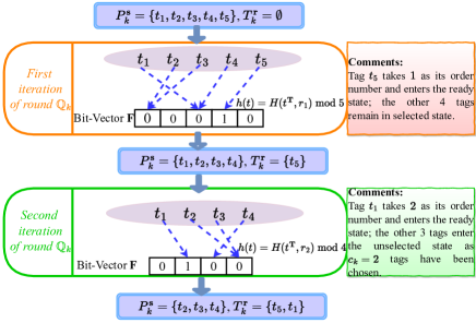
Figure 3: A running example of OPT-C2.

We take an example to show how OPT-C2 runs. Suppose, when round $\mathbb{Q}_{k}$ starts, $5$ tags: $t_{1},t_{2},\cdots,t_{5}$ from category $P_{k}$ stay in the selected state, and $c_{k}=2$. Thus, initially, $P_{k}^{\textbf{s}}=\{t_{1},t_{2},\cdots,t_{5}\}$ and $T_{k}^{\textbf{r}}=\emptyset$. Let’s look at the first iteration of steps 1-5 in round $\mathbb{Q}_{k}$. In step 1, $R$ broadcasts a random seed $r_{1}$ and $|P_{k}^{\textbf{s}}|=5$ to all tags in $P_{k}^{\textbf{s}}=\{t_{1},t_{2},..,t_{5}\}$. Assume that in step 2, the hash values of the $5$ tags are: $h(t_{1})=h(t_{4})=2$, $h(t_{2})=h(t_{3})=0$, and $h(t_{5})=3$. Then, the reader will create a vector $\textbf{F}=[0,0,0,1,0]$ in step 3 and send it out. In step 4, since $\textbf{F}[h(t_{5})]=1$, tag $t_{5}$ takes $1$ as its reporting order and enters the ready state; since $\textbf{F}[h(t_{1})]=\textbf{F}[h(t_{4})]=\textbf{F}[2]=0$, tags $t_{1}$ and $t_{4}$ update their local counter $cnt$ to $1$ and stay in the selected state; since $\textbf{F}[h(t_{2})]=\textbf{F}[h(t_{3})]=\textbf{F}[0]=0$, tags $t_{2}$ and $t_{3}$ do the same thing as $t_{1}$ and $t_{4}$. In step 5, reader $R$ moves $t_{5}$ from $P_{k}^{\textbf{s}}$ to $T_{k}^{\textbf{r}}$ because tag $t_{5}$ is now in the ready state. Lastly in step 6, since $|T_{k}^{\textbf{r}}|=|\{t_{5}\}|=1<c_{k}=2$, $R$ repeats step 1-5. The second iteration is executed similarly to the first. Fig. 3 provides a graphic example of the this process.

Following, we analyze OPT-C.

Theorem 3.5

After round $\mathbb{Q}_{k}$, exactly $c_{k}$ tags are in the ready state, and each of them is assigned a unique reporting order ranging from $1$ to $c_{k}$. Moreover, $T_{k}^{\textbf{r}}$ has the same probability of $1/(_{\,c_{k}}^{n_{k}})$ to be any $c_{k}$-subset of $P_{k}$.

Proof:

First, by step 6 in $\mathbb{Q}_{k}$, we can observe that reader $R$ stops when $T_{k}^{\textbf{r}}$ contains $c_{k}$ tags from $P^{\textbf{s}}_{k}$. Also, since each tag always records the number of tags that move from $P^{\textbf{s}}_{k}$ to $T_{k}^{\textbf{r}}$ in its local counter $cnt$ (step 4 of OPT-C2), it is easy to determine that the counter $cnt$ on each tag takes a unique integer from $\{1,2,\cdots,c_{k}\}$. Thus, when $\mathbb{Q}_{k}$ ends, we can conclude: $|T_{k}^{\textbf{r}}|=c_{k}$ and each tag in $T_{k}^{\textbf{r}}$ is assigned with a unique reporting order.

Second, we analyze the probability that $T_{k}^{\textbf{r}}$ equals to a particular $c_{k}$-subset of $P_{k}^{\textbf{s}}$. Each tag in $P_{k}$ has the same probability of being included in $P_{k}^{\textbf{s}}$, and each tag in $P_{k}^{\textbf{s}}$ has the same probability of being included in $T_{k}^{\textbf{r}}$, so each tag in $P_{k}$ has the same probability of being included in $T_{k}^{\textbf{r}}$. Furthermore, since $P_{k}$ has $(_{\,c_{k}}^{n_{k}})$ different $c_{k}$-subsets, the probability that $T_{k}^{\textbf{r}}$ is equal to a particular $c_{k}$-subset of $P_{k}$ is $1/(_{\,c_{k}}^{n_{k}})$.

∎

Theorem 3.6

Let $|\text{OPT-C2}|$ represent the communication cost of OPT-C2, then we have $|\text{OPT-C2}|\leq\sum\nolimits_{k=1}^{K}{e\times c_{k}}$.

Proof:

Suppose $P_{k}^{\textbf{s}}$ contains $l_{k}$ tags when round $\mathbb{Q}_{k}$ starts. Since OPT-C1 uses a suitable random seed to put tags into $P_{k}^{\textbf{s}}$ (Theorem 3.1), we have $l_{k}\in[c_{k},c_{k}+6\sqrt{c_{k}}]$.

First, let’s look at the first iteration of $\mathbb{Q}_{k}$. In step 1, reader $R$ sends two parameters: $r$ and $|P_{k}^{\textbf{s}}|$ to create hash function $h()$; In step 3, $R$ sends a $|P_{k}^{\textbf{s}}|$-bit vector F. As mentioned earlier in Theorem 3.4, a $(2\log_{2}(|P_{k}^{\textbf{s}}|))$-bit random seed $r$ is sufficient to describe a hash function [40]. So, this costs us $3\log_{2}(|P_{k}^{\textbf{s}}|)+|P_{k}^{\textbf{s}}|\approx|P_{k}^{\textbf{s}}|$ bits.

Next, we analyze the expected number of tags in $P_{k}^{\textbf{s}}$ that are moved to set $T_{k}^{\textbf{r}}$ in the first iteration. For any tag $t\in P_{k}^{\textbf{s}}$, the probability that $t$ occupies the bit $\textbf{F}[h(t)]$ exclusively is $(1-1/|P_{k}^{\textbf{s}}|)^{|P_{k}^{\textbf{s}}|-1}\approx e^{-1}$. Hence, there are on average $e^{-1}|P_{k}^{\textbf{s}}|$ tags that are moved from $P_{k}^{\textbf{s}}$ to $T_{k}^{\textbf{r}}$, and then we have $|P_{k}^{\textbf{s}}|=(1-e^{-1})l_{k}$ and $|T_{k}^{\textbf{r}}|=e^{-1}l_{k}$ at the end of this iteration.

Following a similar analysis as the first iteration, we find that $|P_{k}^{\textbf{s}}|=(1-e^{-1})^{J}l_{k}$, and $|T_{k}^{\textbf{r}}|=\sum\nolimits_{i=1}^{J}e^{-{\color[rgb]{0,0,0}}}{\color[rgb]{0,0,0}(1-e^{-1})^{i-1}}l_{k}$ hold true at the end of the $J$-th iteration, $J\geq 2$. In order to ensure that $|T_{k}^{\textbf{r}}|=c_{k}$ (i.e., exactly $c_{k}$ tags enter the ready state), reader $R$ needs to perform $I$ iterations to make $|P_{k}^{\textbf{s}}|=(1-e^{-1})^{I}l_{k}$ equal to $l_{k}-c_{k}$. The total number of bits transmitted in these $I$ iterations is $\sum\nolimits_{i=0}^{I-1}(1-e^{-1})^{i}l_{k}=e{l_{k}-el_{k}(1-e^{-1})^{I}}=ec_{k}$. Note that the last equality is due to the fact that $I$ satisfies $(1-e^{-1})^{I}l_{k}=l_{k}-c_{k}$. Applying this result to the $K$ rounds $\mathbb{Q}_{1},\mathbb{Q}_{2},...,\mathbb{Q}_{K}$ completes the proof. ∎

3.3 The analysis of OPT-C

OPT-C first executes OPT-C1 and then OPT-C2. So according to Theorem 3.5, OPT-C solves the CIS problem. Its overall communication cost and execution time satisfy the following theorem.

Theorem 3.7

Let $|\text{OPT-C}|$ denote the communication cost of OPT-C, then we have $|\text{OPT-C}|\leq\sum\nolimits_{k=1}^{K}(\log_{2}{(\frac{96}{\log_{2}n_{k}})}+\log_{2}c_{k}+{ec_{k}})$. Moreover, the execution time of OPT-C is within a factor of $\frac{e}{\log_{2}(e)}\approx 1.88$ of the lower bound ${\rm{T}_{{\rm{lb}}}}$ shown in (2).

Proof:

From Theorem 3.4 and 3.6, it is clear that $|\text{OPT-C}|=|\text{OPT-C1}|+|\text{OPT-C2}|\leq\sum\nolimits_{k=1}^{K}(\log_{2}{(\frac{96}{\log_{2}n_{k}})}+\log_{2}c_{k}+{ec_{k}})$. Then, the execution time of OPT-C is less than ${\sum\nolimits_{k=1}^{K}(\log_{2}{(\frac{96}{\log_{2}n_{k}})}+\log_{2}c_{k}+{ec_{k}})}/{96}\times{\rm{T}}_{{\rm{96}}}$, where ${\rm{T}}_{{\rm{96}}}$ is the time cost of transmitting a $96$-bit string from reader $R$ to tags. Since

$$\frac{{{\sum\nolimits_{k=1}^{K}\left(\log_{2}{(\frac{96}{\log_{2}n_{k}})}+\log_{2}c_{k}+{ec_{k}}\right)}}/{96}\times{\rm{T}}_{{\rm{96}}}}{{\sum\nolimits_{k=1}^{K}{\log_{2}(e)c_{k}}}/{96}\times{\rm{T}}_{{\rm{96}}}}$$

$$\approx\frac{{{\sum\nolimits_{k=1}^{K}\left({e}\right)c_{k}}}}{{\sum\nolimits_{k=1}^{K}{\log_{2}(e)c_{k}}}}=\frac{e}{\log_{2}(e)}\approx 1.88,$$

we know that the communication cost of OPT-C is within a fact of $1.88$ of the lower bound. Note that the first approximation in the above derivation is due to the fact that $\frac{\log_{2}{(96/\log_{2}n_{k})}}{c_{k}}<\frac{3.85}{c_{k}}\ll e$ for $\forall k\in\{1,2,...,K\}$, and $\log_{2}(c_{k})\ll c_{k}$.

∎

Hence, the execution time of OPT-C is mainly determined by $K$ and $c_{1},c_{2},...,c_{K}$, it is near-optimal in theory.

4 The Implementation of OPT-C in Real RFID Systems Using COTS Devices

To assess the feasibility and performance of the OPT-C protocol, we have implemented it in a real RFID system, utilizing readily available COTS RFID devices. This implementation, denoted as $\text{OPT-C}_{\mathbf{IMPL}}$, is achieved via reader-end programming without requiring any hardware modifications to the COTS tags. Importantly, $\text{OPT-C}_{\mathbf{IMPL}}$ exclusively relies on tags’ EPCs and the standard Select command, as mandated by the C1G2 standard [37]. This ensures seamless integration into real-world RFID systems. $\text{OPT-C}_{\mathbf{IMPL}}$ encompasses two fundamental functionalities, denoted as F-1 and F-2, which are outlined as follows:

$\bullet$ F-1: Generating Hash Values for Tags without Overburdening COTS Tags: To achieve this function, we conduct a thorough analysis of the bit composition within the 96-bit IDs (EPCs) of COTS tags. This analysis reveals that the IDs of COTS tags typically contain a sufficient number of random bits. Drawing inspiration from established software implementations of hash functions on COTS tags, as found in references [42, 43, 46, 47], we successfully generate the required hash value on each COTS tag. Importantly, this is achieved without imposing any additional computational burden on the COTS tags. Further details are in Section 4.1.

$\bullet$ F-2: Designing an Efficient Algorithm to Generate Appropriate "Select" Commands for Swiftly Selecting Tags with Hash Values Below a Given Threshold $\bm{\tau}$: The straightforward approach to selecting all tags with a hash value no more than $\bm{\tau}$ would involve issuing $\bm{\tau}+1$ individual Select commands, each designated by an integer $i$ ranging from $0$ to $\bm{\tau}$. However, this approach proves time-consuming, requiring $\bm{\tau}$ individual "Select" commands. Therefore, we harness the tag filtering function provided by the "Select" command [37, 42, 43] to design a more efficient method that can generate a significantly smaller number of Select commands for choosing all tags with hash values no more than $\bm{\tau}$. We specifically design a method called SelGen, which can generate no more than $\lceil\log_{2}(\bm{\tau})\rceil+1$ Select commands for selecting all tags with hash values no more than $\bm{\tau}$ from each category $P_{k}$. Further details are in Section 4.2.

$\bullet$ With these core functionalities, we effectively implement the proposed OPT-C protocol in a real RFID system consisting of COTS devices. The details are in Section 4.3.

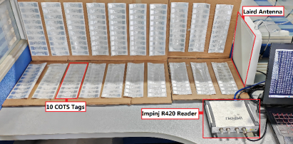
Figure 4: Real-world experimental scenario with densely deployed COTS tags in a small area.

4.1 Generating Hash Values on COTS Tags

This section, we present our approach to generating hash values for COTS tags, a key aspect of the OPT-C protocol. We have observed that the 96-bit IDs (EPCs) of COTS tags typically contain a substantial number of random bits. This observation serves as the foundation for achieving functionality F-1 without requiring any hardware modifications to the COTS tags.

To validate this insight, we conduct practical experiments using an Impinj Speedway R420 reader in conjunction with a diverse set of $200$ COTS tags. This set includes a variety of widely used COTS tags: $100$ ALN-9630 tags, $50$ NXP-Ucode7 tags, and $50$ Impinj-ER62 tags. Fig. 4 shows the real RFID system. After collecting the IDs of these tags, we pursue two critical tasks:

1. Quantification of Entropy for IDs (EPCs): To perform a systematic analysis, we partitioned each tag’s EPC into $24$ subarrays, each comprising $4$ bits. Subsequently, we quantified the empirical entropy of these subarrays, shown in Fig. 5. Notably, the $21$st, $22$nd, $23$rd, and $24$th subarrays exhibit entropies of $3.97$, $3.98$, $3.95$, and $3.94$ bits, respectively. This indicates the presence of more than $3.9$ independently and uniformly distributed random bits in each subarray.

2. Generation of Hash Values from Random Bits: We delineate the approach for generating hash values using these identified random bits. Let $P_{k}$ represent a subset of tags ($k\in\{1,2,\cdots,K\}$), encompassing any $n_{k}$ of the 200 COTS tags, and let $\mathcal{L}=\lceil(\log_{2}(n_{k})\rceil)$. We expound on how to generate a hash value ($h(t)$) for each tag $t\in P_{k}$ using its EPC (composed of $96$ bits denoted as $A[1],A[2],\cdots,A[96]$). It’s noteworthy that the subarrays spanning from the $21$st to the $24$th position ($A[81],A[82],\cdots,A[96]$) are recognized to contain approximately $16$ random bits, which are deemed $16$ independent and uniformly distributed random bits. Consequently, to create the hash value $h(t)$ for tag $t$, we execute the following two steps:
Step 1: Randomly select an integer $\mathcal{I}$ from the range ${81,82,\ldots,96-\mathcal{L}+1}$.
Step 2: Employ the decimal value of the bit array: $A[\mathcal{I}],A[\mathcal{I}+1],\cdots,A[\mathcal{I}+\mathcal{L}-1]$, as the hash value $h(t)$ specific to the tag $t$ in question.

This approach ensures the generation of hash values without overburdening the COTS tags, aligning with the requirements of the OPT-C protocol.

4.2 Efficient Generation of Select Commands for Hash-Based Tag Selection

Building upon the generated hash values in Section 4.1, we propose an approach for the efficient generation of Select commands, designed to select tags in a category $P_{k}$ whose hash values are less than or equal to a specified threshold $\bm{\tau}$. This approach fulfills functionality F-2.

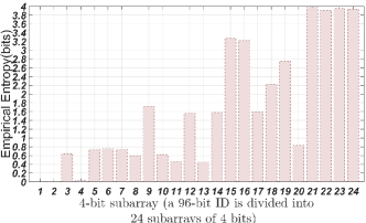
Figure 5: The entropy of $200$ COTS tag IDs.

As defined by the C1G2 standard [37], a COTS RFID reader ($R$) can employ a Select command to specify a particular group of tags for an upcoming tag inventory process. The Select command defines a filter string against which tags are compared to determine if they meet the criteria, and only the matching tags are included in the upcoming inventory. Consequently, for a given threshold value $\bm{\tau}$, reader $R$ can execute $\bm{\tau}+1$ Select commands, each using a filter string $i$ to select tags with hash values equal to $i$, where $i\in\{0,1,\cdots,\bm{\tau}\}$. However, due to the common prefixes shared by hash values within $\{0,1,\cdots,\bm{\tau}\}$ in binary form, the number of Select commands can be significantly reduced. For instance, when using a $4$-bit array to represent the hash value of each tag, a single Select command with the filter string $\mlq\mlq 000*\mrq\mrq$ can select tags with hash values not exceeding 1. This is because the tag with a hash value of $0$ ($\text{0000}_{2}$) and the tag with a hash value of 1 ($\text{0001}_{2}$) share the same unique prefix $\mlq\mlq 000\ast\mrq\mrq$.

To address this optimization, we introduce a method, called SelGen, which generates no more than $\lceil\log_{2}(\bm{\tau})\rceil+1$ Select commands to choose all tags with hash values not exceeding $\bm{\tau}$. Specifically, assume that each tag uses a $\mathcal{L}$-bit array in its EPC memory as its hash value, and $(\tau_{\mathcal{L}},\tau_{\mathcal{L}-1},\cdots,\tau_{1})$ denotes the binary form of $\bm{\tau}$ ($\bm{\tau}=\sum\nolimits_{i=1}^{\mathcal{L}}\tau_{i}2^{i-1}$), the SelGen method proceeds as below:
(1) Reader $R$ initializes an empty set $\mathbb{S}$.
(2) For each $i\in\{\mathcal{L},\mathcal{L}-1,\cdots,1\}$
(3)   If $\tau_{i}=1$, $R$ generates a Select command using $\mlq\mlq\tau_{\mathcal{L}}\tau_{\mathcal{L}-1}\cdots\tau_{i+1}\underbrace{0}_{1}\underbrace{\ast\ast\cdots\ast}_{i-1}\mrq\mrq$ as the filter string and adds this command to $\mathbb{S}$.
(4)   If $\tau_{i-1}=\tau_{i-2}=\cdots=\tau_{1}=1$ or $i=1$, $R$ generates a Select command using

$$\mlq\mlq{\tau_{\mathcal{L}}\tau_{\mathcal{L}-1}\cdots\tau_{i+1}}\underbrace{\tau_{i}}_{1}\underbrace{\ast\ast\cdots\ast}_{i-1}\mrq\mrq$$

as the filter string, adds this command to $\mathbb{S}$, and ends the loop.

The filter strings generated in step (3) of SelGen can select any hash value less than $\bm{\tau}$. This is because, for any value $\bm{x}=(x_{\mathcal{L}},x_{\mathcal{L}-1},\cdots,x_{1})<\bm{\tau}=(\tau_{\mathcal{L}},\tau_{\mathcal{L}-1},\cdots,\tau_{1})$, there exists an index $j\in\{\mathcal{L},\mathcal{L}-1,\cdots,1\}$ such that $\tau_{\mathcal{L}}=x_{\mathcal{L}},\tau_{\mathcal{L}-1}=x_{\mathcal{L}-1},\cdots,\tau_{j+1}=x_{j+1}$, and $\tau_{j}>x_{j}$. Since step (4) shall select the value $\bm{\tau}$, we know that SelGen can ensure the selection of all tags with hash values not exceeding $\bm{\tau}$. Moreover, SelGen generates at most a total of $\sum\nolimits_{i=1}^{\mathcal{L}}{\tau_{i}}+1$ Select commands, corresponding to the number of $\mlq 1\mrq$s in the string $(\tau_{\mathcal{L}},\tau_{\mathcal{L}-1},\cdots,\tau_{1})$ plus one. Therefore, the number of Select commands in $\mathbb{S}$ is no more than $\lceil\log_{2}(\bm{\tau})\rceil+1$.

4.3 Implementation of OPT-C

In this section, we detail the implementation of the OPT-C protocol, denoted as $\text{OPT-C}_{\mathbf{IMPL}}$, using the hash value generation method discussed in Section 4.1 and the Select command generation method (SelGen) explained in Section 4.2.

Let $S$ represent the tag population, which comprises 200 COTS tags categorized into $K$ distinct groups: $P_{1},P_{2},\cdots,P_{K}$. Each category $P_{k}$ contains $n_{k}$ tags selected from the population. The $\text{OPT-C}_{\mathbf{IMPL}}$ implementation is built based on the functionalities F-1 and F-2. Specifically, we first employ the last $16$ bits ($A[81],A[82],\ldots,A[96]$) in each tag’s EPC to generate the hash value, denoted as $h(t)$, for every tag $t$ in a category $P_{k}$, where $k\in\{1,2,\ldots,K\}$. Second, we employ the SelGen method to implement the two main stages of the OPT-C protocol in a real RFID system as follows.

$\bullet$ Implementing the first stage of OPT-C:
The initial stage, OPT-C1, encompasses a coarse sampling process that draws roughly $c_{k}$ tags from each category $P_{k}$ (where $k\in\{1,2,\cdots,K\}$). The primary objective is to select all tags with a hash value that does not exceed the defined threshold $\bm{\tau}=c_{k}+3\sqrt{c_{k}}$. To accomplish this, the reader $R$ generates a hash value for each tag $t$ in $P_{k}$ by extracting $\lceil\log_{2}(n_{k})\rceil$ bits from the tag’s EPC. Subsequently, the SelGen method is invoked with a threshold set at $\bm{\tau}=c_{k}+3\sqrt{c_{k}}$ to create a set of Select commands, designated as $\mathbb{S}_{k}^{\textbf{I}}$, capable of selecting all tags with hash values not exceeding $\bm{\tau}$. $R$ then executes the commands in $\mathbb{S}_{k}^{\textbf{I}}$ to select a set, $P_{k}^{\textbf{s}}$, comprising slightly more than $c_{k}$ tags from $P_{k}$ (refer to Section 3.1 for further details).

$\bullet$Implementing the second stage of OPT-C:
The second stage, OPT-C2, involves a more refined sampling process, which precisely selects $c_{k}$ tags from $P_{k}^{\textbf{s}}$ and assigns them unique reporting orders. To implement OPT-C2, the reader $R$ generates a hash value for each tag $t$ within $P_{k}^{\textbf{s}}$ by extracting a hash value containing $\log_{2}(|P_{k}^{\textbf{s}}|^{2})\leq 2\log_{2}(c_{k}+6\sqrt{c_{k}})$ random bits from the tag’s EPC. Subsequently, $R$ leverages the SelGen method to produce a set of Select commands, denoted as $\mathbb{S}_{k}^{\textbf{II}}$, which selectively pick precisely $c_{k}$ tags from $P_{k}^{\textbf{s}}$. Each chosen tag is implicitly assigned a unique reporting order in the form of a unique integer. Finally, $R$ executes the commands within $\mathbb{S}_{k}^{\textbf{II}}$ to select exactly $c_{k}$ tags from $P_{k}^{\textbf{s}}$. Please note that these $c_{k}$ tags constitute the set $T_{k}^{\textbf{r}}$ (see Section 3.2).

5 Simulations

In this section, we evaluate OPT-C’s performance with two state-of-the-art category information sampling protocols: TPS [6] and ACS [7]. We also verify Theorem 3.2 using $96$-bit IDs from the universe $U$ to show that reader $R$ can find a suitable random seed rapidly in practice.

All simulations are conducted based on the C1G2 standard [37] to measure communication times for the tested protocols. Our setup includes a transmission rate of $26.7$ kbps from reader $R$ to the tags, with a $302\mu$s interval between consecutive transmissions. Therefore, reader $R$ requires $\rm{T}_{\rm{96}}=3897.5\times 10^{-6}$s to transmit a 96-bit string to the tags. Subsequently, the time needed to send an $f$-bit string to the tags was $\frac{f\rm{T}_{\rm{96}}}{96}$s.

We refrain from evaluating the success probability, specifically the likelihood that at least one of the $c_{k}$ sampled tags from $P_{k}$ is not missing. This is because all three protocols exhibit the same success probability while demonstrating distinct execution times with identical reliability numbers. However, in cases where an equal running time budget is assigned to all tested protocols, OPT-C surpasses others in success probability. This is attributed to its capability to sample a greater number of tags within the same time frame, as depicted in Figs. 6, 7, 8, and 11.

5.1 Simulation results for execution times

Fig. 6 shows the results of the three protocols in Scenarios 1 and 2. Please note that the lower bound $\rm{T}_{\rm{lb}}$ in the two figures is drawn according to (2) in Theorem 2.2. From this figure, we can observe: (1) the execution time of OPT-C increases with $K$, which is consistent with its theoretical time shown in Theorem 3.7; and (2) the execution time of OPT-C is significantly less than the other protocols, and is actually close to the lower bound of execution time. For example, in Scenario 1, when $K=100$ (the number of categories is $100$) the execution times of OPT-C, ACS, and TPS are $1.5$s, $3.3$s and $6.1$s, respectively; in Scenario 2, when $K=100$, the execution times of OPT-C, ACS, and TPS are $0.6$s, $1.2$s and $2.2$s, respectively. Generally, in Scenarios 1 and 2, OPT-C reduces the execution time by a factor of about $2.1$, and is within about $1.88$ times of the lower bound $\rm{T}_{\rm{lb}}$.

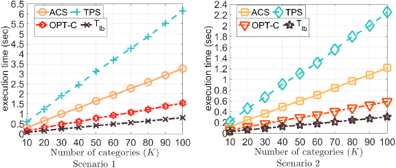
Figure 6: Performance comparisons for Scenarios 1 and 2 with varied $K$ (the number of categories).

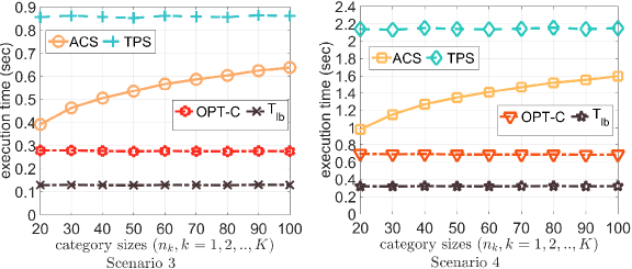
Figure 7: Performance comparisons for Scenarios 3 and 4 with varied $n_{1},n_{2},...,n_{K}$ (category sizes).

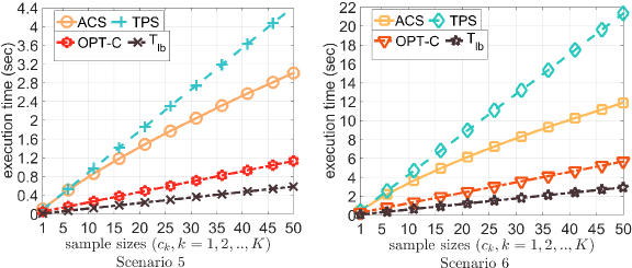
Figure 8: Performance comparisons for Scenarios 5 and 6 with varied sample size $c_{k},k=1,2,...,K$.

Next, for Scenarios 3 and 4, we show the results of the three protocols in Fig. 7. This figure tells: (1) the execution time of OPT-C remains unchanged with the increase of the $K$ category sizes, which is consistent with its theoretical time shown in Theorem 3.7; and (2) the execution time of OPT-C is much less than other protocols, and close to the lower bound. For example, in Scenario 3, when $n_{1}=n_{2}=\cdots=n_{K}=100$, the execution times of OPT-C, ACS, and TPS are $0.3$s, $0.6$s and $0.8$s, respectively; in Scenario 4, when $n_{1}=n_{2}=\cdots=n_{K}=100$, the execution times of OPT-C, ACS, and TPS are $0.7$s, $1.6$s and $2.2$s, respectively. Generally, in Scenarios 3 and 4, OPT-C reduces the execution time by a factor of about $2.2$, and is within about $1.88$ times of the lower bound $\rm{T}_{\rm{lb}}$.

Lastly, for Scenarios 5 and 6, we show the results of the three protocols in Fig. 8. This figure demonstrates: (1) the execution time of OPT-C increases with the $K$ sample sizes, which is also indicated by its theoretical time shown in Theorem 3.7; and (2) the execution time of OPT-C is much less than other protocols, and is close to the lower bound. For example, in Scenario 5, when $c_{1}=c_{2}=\cdots=c_{K}=50$, the execution times of OPT-C, ACS, and TPS are $1.1$s, $3$s and $4.4$s, respectively; in Scenario 6, when $n_{1}=n_{2}=\cdots=n_{K}=100$, the execution times of OPT-C, ACS, and TPS are $5.7$s, $11.9$s and $21.3$s, respectively. Overall for Scenarios 5 and 6, OPT-C reduces the communication time by a factor of about $2.6$, and is within about $1.88$ times of the lower bound $\rm{T}_{\rm{lb}}$.

The experimental results of scenarios 1-6 show that OPT-C significantly outperforms the other two protocols in terms of execution time and can approach the lower bound $\rm{T}_{\rm{lb}}$. This verifies the theoretical result in Theorem 3.7. There are two reasons why OPT-C is superior: its novel coarse sampling protocol, which can select a little more than $c_{k}$ tags from each category $P_{k}$ at an almost negligible time cost (see Theorem 3.4), and its refined sampling protocol, which can extract exactly $c_{k}$ tags from these already selected tags with a time cost that is near the lower bound (Theorem 3.6).

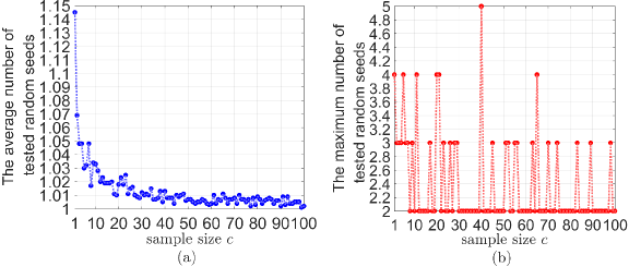
Figure 9: The number of tested random seeds in Scenario 7 ($n=10^{3}$, $c\in\{1,2,\cdots,100\}$) for the basic sampling problem. (a) Average Number. (b) Maximum Number.

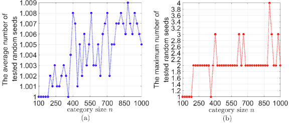
Figure 10: The number of tested random seeds for Scenario 8 ($c=50$, $n\in\{100,120,\cdots,10^{3}\}$) for the basic sampling problem. (a) Average Number. (b) Maximum Number.

5.2 Verifying Theorem 3.2

We investigate the number of tests required by reader $R$ to find a suitable random seed (in OPT-C1) with $96$-bit ID from the universe $U$, in order to verify two facts: (1) the probability of finding a suitable one within $6$ tests is close to $1$; and (2) the average number of tests required is under $2.5$ (i.e., to verify Theorem 3.2). In particular, we compute how many random seeds should be tested in order to solve the basic sampling problem of selecting at least $c$ and at most $c+6\sqrt{c}$ tags randomly from a single category $P$ of $n$ tags. Any $n$-subset of $U$ can be $P$. Given fixed values of $c$ and $n$, we conduct $10^{3}$ independent trials to calculate the actual numbers of tested random seeds for finding a suitable one. Each trial includes $6$ steps:

1. Initialize a variable $x$ to be $0$.

2. Generate the category $P$ by randomly choosing $n$ tags from the universe $U$ (i.e., choosing $n$ IDs from the $2^{96}$ different IDs).

3. Pick a random seed $r$, and compute the corresponding hash values $H(t,r)\bmod n=h(t)$ for each tag $t\in P$.

4. A tag $t\in P$ enters the selected state if $h(t)\leq c+3\sqrt{c}$.

5. Calculate the value of $l$, which represents the number of tags that enter the selected state

6. If $l\in[c,c+6\sqrt{c}]$, stop the trial and report the value of $x$; otherwise, set $x=x+1$ and return to step (3).

We conduct $10^{3}$ trials in two typical scenarios, referred to as Scenario 7 and Scenario 8. These scenarios feature varying relationships between the parameters $n$ and $c$. Scenario 7 maintains $n$ at $10^{3}$ and increases $c$ from $1$ to $10^{2}$, while Scenario 8 keeps $c$ at $50$ and varies $n$ from $10^{2}$ to $10^{3}$. The results for Scenarios 7 and 8 are presented in Fig. LABEL:fig_for_sc5_experiment and 9, respectively. These figures reveal that the average number of tested random seeds is below $1.15$, and the maximum is always under $6$, thereby verifying Theorem 3.2 in practice.

6 Experimental Results

In this section, we present the results of our experiments aimed at evaluating the real-world performance of the $\text{OPT-C}_{\mathbf{IMPL}}$ protocol against state-of-the-art C1G2-compatible sampling protocols within a real RFID system. These experiments are conducted using an Impinj R420 reader, denoted by $R$, and a collection of $200$ COTS tags, specifically ALN-9630, NXP-Ucode7, and Impinj-ER62, all of which are compliant with the C1G2 standard [37].

Our experimental setup involves integrating the Impinj R420 reader with a 900 MHz Laird polarized antenna. This reader, $R$, operates in dense Miller 8 mode and is connected to a laptop computer equipped with an Intel i7-7700 processor and 16GB of RAM via an Ethernet connection. Varying quantities of tags, ranging from 40 to 200, are placed at a distance of approximately 1.5 meters from the antenna. For a visual representation of the physical configuration of the RFID system, please refer to Fig. 4. The implementation of $\text{OPT-C}_{\mathbf{IMPL}}$ is carried out in C# using the Octane SDK .NET 4.0.0 [41], running on the laptop to control the reader for tag recognition.

Our investigation of existing literature on RFID tag sampling [48, 46, 47, 6, 7] leads us to identify the DTS protocol proposed in [48] as the sole state-of-the-art tag sampling protocol that can be directly implemented on COTS RFID devices (i.e., fully C1G2-compatible). The DTS protocol facilitates the random selection of tags from a subset with user-specified probabilities. However, the DTS protocol cannot guarantee to select precisely $c_{k}$ tags from each category $P_{k}$ ($k=1,2,\cdots,K$), as each tag is independently chosen with a fixed probability. This leads to the possibility of selecting more than $c_{k}$ tags in practice (as discussed in section 4.2.2 of [48]). To address this, we enhance the DTS protocol by introducing a trimming mechanism to deselect surplus tags when more than $c_{k}$ tags are chosen from category $P_{k}$, ensuring equitable comparisons. In addition to DTS, we design a baseline tag sampling protocol called RandomSelect. This protocol selects each sampled tag using an individual Select command, and is fully C1G2-compatible.

TABLE V: Parameter settings for the three real scenarios

Real Scenario	The number of categories	Category sizes	Sample sizes
I	$K$ $\in\{2,4,...,10\}$	$n_{1}=n_{2}=...=n_{K}=20$	$c_{1}=c_{2}=...=c_{K}=5$
II	$K=8$	$n_{1}=n_{2}=...=n_{K}\in\{10,15,20,25\}$	$c_{1}=c_{2}=...=c_{K}=4$
III	$K=8$	For each $k\in\{1,2,...,K\}$, if $k\bmod 2=1$, $n_{k}=20$; if $k\bmod 2=0$, $n_{k}=30$	$c_{1}=c_{2}=...=c_{K}\in\{2,4,6,8,10\}$

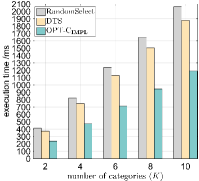
(a) Real Scenario I

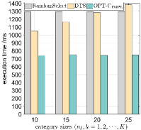
(b) Real Scenario II

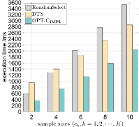
(c) Real Scenario III

Figure 11: The practical communication time of RandomSelect, DTS, and $\text{OPT-C}_{\mathbf{IMPL}}$ for Real Scenarios I, II, and III.

We access the performance of the three protocols (RandomSelect, DTS, and $\text{OPT-C}_{\mathbf{IMPL}}$) in $3$ typical real scenarios (Scenarios I-III). Each scenario is characterized by variations in one of three key parameters, which include $K$ (the number of categories), $n_{1},n_{2},\cdots,n_{K}$ (category sizes), and $c_{1},c_{2},\cdots,c_{K}$ (sample sizes or reliability numbers). The detailed parameter settings for Scenarios I-III are listed in Tab. V. For each scenario, we conduct 10 trials and record the average practical execution times of the three protocols. Here’s how we conduct the trials in each scenario:

$\bullet$ Step 1: We manually pick $N=\sum\nolimits_{k=1}^{K}n_{k}$ tags from the universe $\mathcal{T}$ of $500$ COTS tags and divide them into $K$ categories: $P_{1},P_{2},\cdots,P_{K}$, where $P_{k}$ contains $n_{k}$ tags ($k=1,2,\cdots,K$) assigned with the same category-ID $k$.

$\bullet$ Step 2: We let the reader $R$ execute one of the three tested protocols over this tag population to sample $c_{k}$ tags from each category $P_{k}$ and assign unique integers to the sampled tags. We record the time taken by each protocol.

$\bullet$ Step 3: The reader $R$ pauses and waits for us to manually select another $N$ tags from $\mathcal{T}$ for the next trial.

The experimental results from these three real scenarios offer substantial evidence supporting the superior performance of $\text{OPT-C}_{\mathbf{IMPL}}$. In particular, Fig. 11 demonstrates that $\text{OPT-C}_{\mathbf{IMPL}}$ consistently outperformed DTS and RandomSelect in terms of average communication time. For instance, in Scenario I, $\text{OPT-C}_{\mathbf{IMPL}}$ achieves approximately $63\%$ of DTS’s average communication time and $57\%$ of RandomSelect’s average communication time. Similar trends can be observed in Scenarios III and V, where $\text{OPT-C}_{\mathbf{IMPL}}$ outperforms DTS and RandomSelect, achieving around $62\%$ and $57\%$ of their respective average communication times.

The superior performance of $\text{OPT-C}_{\mathbf{IMPL}}$ can be attributed to the OPT-C protocol, which offers two key advantages: (1) Coarse Sampling Stage: $\text{OPT-C}_{\mathbf{IMPL}}$ follows the first stage of OPT-C, employing a specially designed threshold and tag hash values. This allows $\text{OPT-C}_{\mathbf{IMPL}}$ to sample slightly more than $c_{k}$ tags from category $P_{k}$ using fewer than $\lceil\log_{2}(c_{k})\rceil+1$ Select commands. (2) Refined Sampling Stage: $\text{OPT-C}_{\mathbf{IMPL}}$ follows the second stage of OPT-C, using a specifically designed hash value range and threshold. This enables $\text{OPT-C}_{\mathbf{IMPL}}$ to draw exactly $c_{k}$ tags from category $P_{k}$ and assign them unique reporting orders using fewer than $2\lceil\log_{2}(c_{k})\rceil+2$ Select commands.

In summary, the number of Select commands used by $\text{OPT-C}_{\mathbf{IMPL}}$ for the CIS problem is at most $\sum\nolimits_{k=1}^{K}(3\lceil\log_{2}(c_{k})\rceil+3)$, with each Select command employing a filter string of $O(\log_{2}(c_{k}))$ bits. In contrast, the state-of-the-art DTS protocol [48] demands approximately $\sum\nolimits_{k=1}^{K}O(\sqrt{c_{k}})$ Select commands and an additional operation involving pre-writing a lengthy bit-vector into each tag’s user memory before sampling tags. The RandomSelect protocol necessitates $\sum\nolimits_{k=1}^{K}c_{k}$ Select commands, each utilizing a $96$-bit array as its mask.

7 Conclusions

In this paper, we have studied the Category Information Sampling Problem in practical RFID systems with missing tags. Our primary objective is to use the shortest possible time to randomly select a few tags from each group and collect their category information. For this target, we first obtained a lower bound on the execution time for solving this problem. Then, we presented a near-optimal protocol OPT-C, and proved that OPT-C can solve the studied problem with an execution time close to the lower bound. Lastly, we verified the practicability and validity of OPT-C with real experiments, and compared OPT-C with the state-of-the-art solutions through extensive simulations to demonstrate its superiority.

Xiujun Wang received the B.E. degree in computer science and technology, from Anhui Normal University, and the Ph.D. degree in computer software and theory, from University of Science and Technology of China. He is currently an Associate Professor at the School of Computer Science and Technology, Anhui University of Technology. His research interest includes data stream processing, randomized algorithm, and Internet of Things.

Zhi Liu (SM’11-M’14-SM’19) received the B.E. degree from the University of Science and Technology of China, China, and the Ph.D. degree in informatics in National Institute of Informatics, Japan. He is currently an Associate Professor at The University of Electro-Communications, Tokyo, Japan. His research interest includes video network transmission, vehicular networks and mobile edge computing. He was the recipient of the multiple IEEE best paper awards. He is a senior member of IEEE.

Xiaokang Zhou (M-12) is currently an associate professor with the Faculty of Data Science, Shiga University, Japan. He received the Ph.D. degree in human sciences from Waseda University, Japan, in 2014. From 2012 to 2015, he was a research associate with the Faculty of Human Sciences, Waseda University, Japan.

Yong Liao is a professor in the school of cyberspace science and technology at University of Sciences and Technology of China. He received his PhD degree from University of Massachusetts Amherst in 2010. Before that he graduated from Institute of Software, Chinese Academy of Sciences with a master¡¯s degree, and University of Science and Technology of China with a bachelor¡¯s degree, in 2004 and 2001, respectively.

Han Hu is currently a Professor in Beijing Institute of Technology, China. He received the B.E. and Ph.D. degrees from the University of Science and Technology of China, China, in 2007 and 2012 respectively. His research interests include multimedia networking. He received several academic awards, including Best Paper Award of IEEE TCSVT 2019, Best Paper Award of IEEE Multimedia Magazine 2015, Best Paper Award of IEEE Globecom 2013, etc.

Xiao Zheng received the B.S. degree from Anhui University, China, in 1997, the M.S. degree from Zhejiang University of Science and Technology, China, in 2003, and the Ph.D. degree in computer science and technology from Southeast University, China, in 2014. He is currently a Professor with Anhui University of Technology, China and the Director of Anhui Engineering Research Center for Intelligent Applications and Security of Industrial Internet.

Jie Li (Senior Member, IEEE) received the Dr. Eng degree from the University of Electro-Communications, Tokyo, Japan. Dr. Jie Li is an Endowed Chair Professor in Computer Science and Engineering, School of Electronic Information and Electrical Engineering, Director of Intelligent Big Data System (iBDSys) Lab., Director of SJTU Blockchain Research Centre, Adjunct Professor of Zhiyuan College with Zhiyuan Honors Program and SJTU Paris Elite Institute of Technology (SPEIT), Shanghai Jiao Tong University (SJTU), Shanghai, China. He is a Foreign Fellow, Engineering Academy of Japan (EAJ) (2019). He was a full Professor in Department of Computer Science, University of Tsukuba, Japan. He was a visiting Professor in Yale University, USA, Inria Sophia Antipolis and Inria Grenoble-Rhone-Aples, France, during the sabbatical year in September 2014 through August 2015. He has been a visiting Professor/Adjunct Professor of The Chinese University of Hong Kong (CUHK), The Hong Kong Polytechnical University (PolyU), City University of Hong Kong, Tsinghua University, and University of Science and Technology of China (USTC). His current research interests are in Big Data, AI, Blockchain, network systems and security, and smart city.

A.   An analytical calculation of $c_{k}$ to guarantee a given success probability

Assume that $\alpha_{k}\in(0,1)$ represents the rate of missing tags in category $P_{k}$, which can be estimated very rapidly with a time cost of only $O(\log_{2}(\log_{2}(|P_{k}|))$ [32]. When only one tag is selected randomly from $P_{k}$, the success probability is $1-\alpha_{k}$, i.e., the probability that the randomly selected tag is not missing is $1-\alpha_{k}$. However, if we choose $c_{k}$ tags randomly from $P_{k}$, the success probability increases rapidly to $1-\frac{(\alpha_{k}|P_{k}|)^{\underline{c_{k}}}}{|P_{k}|^{\underline{c_{k}}}}\geq 1-{\alpha_{k}}^{c_{k}}$. This can be explained as follows: as long as one of the $c_{k}$ randomly selected tags from $P_{k}$ is not missing, we can successfully collect $P_{k}$’s category information. So the success probability is equal to the probability that at least one of the $c_{k}$ randomly selected tags is not missing (i.e., equal to $1-\frac{(\alpha_{k}|P_{k}|)^{\underline{c_{k}}}}{|P_{k}|^{\underline{c_{k}}}}$). Furthermore, given a small $\varepsilon\in(0,1)$, to guarantee a high success probability of $1-\varepsilon$, we only need to randomly choose $c_{k}=\ln(\frac{1}{\varepsilon})/\ln(\frac{1}{\alpha_{k}})$, because ${\alpha_{k}}^{c_{k}}={\alpha_{k}}^{\ln(\frac{1}{\varepsilon})/\ln(\frac{1}{\alpha_{k}})}=\varepsilon$. In addition, based on the inequality (4) of Ref. [52]: $\ln(1+z)\leq\frac{2z}{2+z},\text{ $-1<z\leq 0$}$, we can obtain that $\ln(\frac{1}{\alpha_{k}})\geq\frac{2(1-\alpha_{k})}{1+\alpha_{k}}$. Subsequently, since $c_{k}=\ln(\frac{1}{\varepsilon})/\ln(\frac{1}{\alpha_{k}})\leq\ln(\frac{1}{\varepsilon})\frac{1+\alpha_{k}}{2(1-\alpha_{k})}$, we can observe that $c_{k}$ remains small even when $\alpha_{k}$ is relatively large and $\varepsilon$ is relatively small.

B.   Proof of the inequality: $\eqref{number_of_partitions_handled_by_v1}\leq\eqref{number_of_partitions_handled_by_v2}$

Clearly, (4) can be represented by a function $\mathrm{g}(s^{v}_{1,0},s^{v}_{1,1},...,s^{v}_{k,c_{k}})$ of variables: $s^{v}_{k,i}$, $k\in\{1,2,\cdots,K\}$, $i\in\{0,1,\cdots,c_{k}\}$. Note that category sizes $n_{1},n_{2},\cdots,n_{K}$ and reliability numbers $c_{1},c_{2},\cdots,c_{K}$ are pre-given. Furthermore, $\mathrm{g}(s^{v}_{1,0},s^{v}_{1,1},...,s^{v}_{k,c_{k}})$ can be expressed as the product of $K$ functions: $f(s^{v}_{k,0},s^{v}_{k,1},\cdots,s^{v}_{k,c_{k}})=\frac{(s^{v}_{k,0})^{n_{k}-c_{k}}}{(n_{k}-c_{k})!}\prod\nolimits_{i=1}^{c_{k}}s^{v}_{k,i}$, $k\in\{1,2,...,K\}$. We can find the maximum value of each of the $K$ functions by studying the following maximization problem.

$$\max\,\,{\color[rgb]{0,0,0}\ln(f(s^{v}_{k,0},s^{v}_{k,1},\cdots,s^{v}_{k,c_{k}}))}$$

$$s.t.\quad\begin{cases}\sum\nolimits_{i=0}^{c_{k}}s^{v}_{k,i}=\Upsilon-\sum\nolimits_{j=1}^{k-1}n_{j},\\ s^{v}_{k,i}\geq 0\quad(i=0,1,\cdots,c_{k}).\end{cases}$$

Clearly, the function $\ln(f(s^{v}_{k,0},s^{v}_{k,1},\cdots,s^{v}_{k,c_{k}}))=\ln(\frac{(s^{v}_{k,0})^{n_{k}-c_{k}}}{(n_{k}-c_{k})!})+\sum\nolimits_{i=1}^{c_{k}}\ln(s^{v}_{k,i})=(n_{k}-c_{k})\ln({s^{v}_{k,0}})+\sum\nolimits_{i=1}^{c_{k}}\ln(s^{v}_{k,i})-\ln({(n_{k}-c_{k})!})$ is a non-negative linear combination of $c_{k}+1$ concave functions: $\ln({s^{v}_{k,0}})$, $\ln(s^{v}_{k,1})$, $\ln(s^{v}_{k,2})$, $\cdots$, $\ln(s^{v}_{k,c_{k}})$. Thus, $\ln(f(s^{v}_{k,0},s^{v}_{k,1},\cdots,s^{v}_{k,c_{k}}))$ is also concave [35]. So we can use the method of Lagrange multipliers to discover that its maximum value is $({n_{k}-c_{k}})\ln((n-c_{k})\frac{\Upsilon-\sum\nolimits_{j=1}^{k-1}n_{j}}{n_{k}})+\sum\nolimits_{i=1}^{c_{k}}\ln(\frac{\Upsilon-\sum\nolimits_{j=1}^{k-1}n_{j}}{n_{k}})--\ln({(n_{k}-c_{k})!})$, which is obtained when $s^{v}_{k,i}=\frac{\Upsilon-\sum\nolimits_{j=1}^{k-1}n_{j}}{n_{k}}$, $i=1,2,\cdots,n_{k}$, and $s^{v}_{k,0}=(n-c_{k})\frac{\Upsilon-\sum\nolimits_{j=1}^{k-1}n_{j}}{n_{k}}$. Since function $\ln(x)$ is monastically increasing, we know

$$f(s^{v}_{k,0},s^{v}_{k,1},\cdots,s^{v}_{k,c_{k}})\leq\frac{(n_{k}-c_{k})^{n_{k}-c_{k}}}{(n_{k}-c_{k})!}\big{(}\frac{\Upsilon-\sum\nolimits_{j=1}^{k-1}n_{j}}{n_{k}}\big{)}^{n_{k}}$$

. Multiplying the maximum values of the $K$ functions together gives us

$$\prod\nolimits_{k=1}^{K}\left[\frac{(n_{k}-c_{k})^{n_{k}-c_{k}}}{(n_{k}-c_{k})!}\left(\frac{\Upsilon-\sum\nolimits_{j=1}^{k-1}n_{j}}{n_{k}}\right)^{n_{k}}\right]=\Phi,$$

which is the maximum of $\mathrm{g}(s^{v}_{1,0},s^{v}_{1,1},...,s^{v}_{k,c_{k}})$. This leads to the inequality $\eqref{number_of_partitions_handled_by_v1}\leq\eqref{number_of_partitions_handled_by_v2}$.

C.   Proof of the fact: $\mu(c_{k})=e^{3\sqrt{c_{k}}}(1+\frac{3\sqrt{c_{k}}}{c_{k}+3\sqrt{c_{k}}})^{-c_{k}-6\sqrt{c_{k}}}$ is a monotonically decreasing function of $c_{k}$

Let $x=\sqrt{c_{k}}$, then the function $\mu(c_{k})$ can be rewritten as: $\mu(x^{2})=e^{3x}(1+\frac{3x}{x^{2}+3x})^{-x^{2}-6x}=e^{3x+({-x^{2}-6x})\ln(1+\frac{3x}{x^{2}+3x})}$. Since $c_{k}\geq 1$ and $x\geq 1$, proving that the derivative of $\mu(x)$ is less than $0$ will be enough to show $\mu(c_{k})$ is a monotonically decreasing function. The derivative of $\mu(x)$ is analyzed as below:

$${d\,\mu(x)}/{d\,x}=3-(2x+6)\ln(1+{3x}/({x^{2}+3x}))$$

$$\,-({x^{2}+6x})\frac{{x^{2}+3x}}{{x^{2}+6x}}\frac{(2x+6)(x^{2}+3x)-(x^{2}+6x)(2x+3)}{(x^{2}+3x)^{2}}$$

$$\leq\frac{6x+9}{x+3}-\frac{12}{2+3/({x+3})}=\frac{{{-27}}}{(x+3)(2x+9)}<0.$$

The first inequality in the above derivation is based on the inequality (3) of Ref. [52]: $\ln(1+z)\geq\frac{2z}{2+z},\text{$0\leq z<\infty$ }$.

D.   Proof of the fact: $\rho(c_{k})=e^{-3\sqrt{c_{k}}}(1+\frac{-3\sqrt{c_{k}}}{c_{k}+3\sqrt{c_{k}}})^{{\color[rgb]{0,0,0}-c_{k}}}$ is a monotonically decreasing function of $c_{k}$

Let $x=\sqrt{c_{k}}$, then the function $\rho(c_{k})$ can be rewritten as $\rho(x^{2})=e^{-3x+x^{2}(\ln(\frac{x^{2}+3x}{x^{2}}))}$. So, since $c_{k}\geq 1$ and $x\geq 1$, proving that the derivative of $\rho(x)$ is less than $0$ will be enough to show $\rho(c_{k})$ is a monotonically decreasing function. The derivative of $\rho(x)$ is analyzed as below

$${d\,\rho(x)}/{d\,x}=-3+2x\ln\big{(}\frac{x^{2}+3x}{x^{2}}\big{)}$$

$$\quad\quad\quad\quad\quad+x^{2}\frac{x^{2}}{x^{2}+3x}\frac{(2x+3)x^{2}-2x(x^{2}+3x)}{x^{4}}$$

$$\leq-3+2x\left(\frac{\frac{3}{x}}{2}\cdot\frac{2+\frac{3}{x}}{1+\frac{3}{x}}\right)-\frac{3x}{x+3}=0.$$ (11)

The inequality in the above derviation is from the inequality (3) of Ref. [52]: $\ln(1+z)\leq\frac{z}{2}\cdot\frac{2+z}{1+z},\text{ $0\leq z<\infty$ }$.

E. The Select command

According to the C1G2 standard, the reader $R$ is capable of using a Select command to pick a specific group of tags for the upcoming tag inventory. Every tag has a flag variable SL, and the Select command will turn the SL of matched tags to asserted (true) and the SL of unmatched tags to deasserted (false). Only the asserted tags will remain active and respond to reader $R$ in the upcoming tag inventory. A Select consists of six mandatory fields, which are explained below.
$\bullet$ The Target field allows the reader to modify the tag’s SL flag or inventory flag. In $\text{OPT-C}_{\mathbf{IMPL}}$, the reader $R$ sets Target$=100_{2}$ to change the SL flag.
$\bullet$ The Action field specifies the action to be executed by the tag. There are eight different action codes available in Table 6-30 of [37]. In $\text{OPT-L}_{\mathbf{IMPL}}$, the reader $R$ sets Action to be $0$. This means that the matched tags shall assert SL, while the unmatched tags shall deassert SL.
$\bullet$ The MemBank field indicates the memory bank to which a tag will look for comparison with the Mask. As the hash values are stored in EPC memory, reader $R$ sets MemBank$=1$.
$\bullet$ The Pointer field records the starting bit in the selected MemBank, and the Mask will be compared to the bit string starting at this position.
$\bullet$ The Length field specifies the length of the Mask in bits.
$\bullet$ The Mask is a user-specific bit-string that must match the content of a specific position in a MemBank.

Overall, a tag will compare Mask with the Length-bit long string that starts at the Pointer-th bit in its MemBank to determine whether it is a matched or unmatched tag.

F. Explanation of Lower Bound Factors

The lower bound on execution time in Theorem 2.2 is predominantly influenced by two key factors: the number of categories, denoted as $K$, and the reliability numbers $c_{1},c_{2},\ldots,c_{K}$. Here, $K$ signifies the number of different categories (disjoint subsets) in the tag population $S$ and is a crucial parameter characterizing the distributional information of $S$. On the other hand, $c_{k}$ ($k\in\{1,2,\ldots,K\}$) specifies the number of tags that the system user intends to randomly draw from category $P_{k}$ and assign unique reporting orders to. To elaborate on this result, consider the following points:

• The reliability numbers $c_{k}$ ($k\in\{1,2,\ldots\}$) directly impact the lower bound. The larger the number of tags that reader $R$ needs to draw from $P_{k}$ and assign unique reporting orders to, the greater the amount of information $R$ must transmit to handle these selected tags. For example, informing $100$ tags of a unique reporting order from $\{1,2,\ldots,100\}$ is typically more challenging than informing $10$ tags with unique reporting orders from ${1,2,\ldots,10}$ since the former encompasses the latter as a subproblem.

• Another significant factor contributing to the lower bound is $K$, representing the number of categories. As the reader needs to process an increasing number of categories, more information must be transmitted by $R$ to handle each category effectively. For instance, sampling $1$ tag from each of $100$ categories is generally more complex than sampling $1$ tag from each of $10$ categories, as the former includes the latter as a subproblem.

Please note that the parameters $n_{1},n_{2},\ldots,n_{K}$ (representing the number of tags contained in each of the $K$ categories) do not significantly influence the lower bound. The fact that the lower bound on communication time mainly depends on $K$, $c_{1},c_{2},\ldots,c_{K}$ indicates that the primary overhead of the sampling problem potentially lies in the communication cost of assigning the $c_{k}$ randomly selected tags from $P_{k}$ unique reporting orders from $\{1,2,\ldots,c_{k}\}$ (as specified in Requirement (II) of Definition 2.1 in the manuscript). This insight has further guided us to develop a two-stage protocol to address the sampling problem in Section 3. In the first stage, roughly $c_{k}$ tags are drawn from $P_{k}$ with minimal communication cost. Subsequently, in the second stage, a unique reporting order is assigned to exactly $c_{k}$ of these previously selected tags.

References

- [1] F. Bernardini, A. Buffi, D. Fontanelli, D. Macii, V. Magnago, M. Marracci, A. Motroni, P. Nepa, and B. Tellini, “Robot-based indoor positioning of uhf-rfid tags: The sar method with multiple trajectories,” IEEE Transactions on Instrumentation and Measurement, vol. 70, pp. 1–15, 2021.
- [2] K. Ngamakeur, S. Yongchareon, J. Yu, and S. U. Rehman, “A survey on device-free indoor localization and tracking in the multi-resident environment,” ACM Computing Surveys (CSUR), vol. 53, no. 4, pp. 1–29, 2020.
- [3] T. Liu, C. Wang, L. Xie, J. Ning, T. Qiu, F. Xiao, and S. Lu, “Rf-protractor: Non-contacting angle tracking via cots rfid in industrial iot environment,” in IEEE INFOCOM 2022-IEEE Conference on Computer Communications. IEEE, 2022, pp. 390–399.
- [4] H. Wang, S. Chen, and W. Gong, “Artifact: Mobility improves accuracy: Precise robot manipulation with cots rfid systems,” in 2021 IEEE International Conference on Pervasive Computing and Communications Workshops and other Affiliated Events (PerCom Workshops). IEEE, 2021, pp. 436–437.
- [5] H. Cai, G. Wang, X. Shi, J. Xie, M. Wang, C. Qian, and S. Chen, “When Tags ‘Read’ Each Other: Enabling Low-cost and Convenient Tag Mutual Identification,” ACM Transactions on Sensor Networks (TOSN), vol. 18, no. 2, pp. 1–22, 2022.
- [6] J. Liu, S. Chen, Q. Xiao, M. Chen, B. Xiao, and L. Chen, “Efficient information sampling in multi-category rfid systems,” IEEE/ACM Transactions on Networking, vol. 27, no. 1, pp. 159–172, 2018.
- [7] C. Chu, J. Niu, H. Ma, J. Su, R. Xu, and G. Wen, “An efficient information sampling method for multi-category rfid systems,” IEEE Wireless Communications Letters, 2021.
- [8] ”Wireless Identification and Sensing Platform WISP”. [Online]. Available: https://sites.google.com/uw.edu/wisp-wiki/home
- [9] X. Xie, X. Liu, K. Li, B. Xiao, and H. Qi, “Minimal perfect hashing-based information collection protocol for rfid systems,” IEEE Transactions on Mobile Computing, vol. 16, no. 10, pp. 2792–2805, 2017.
- [10] Liu, Xuan and Yin, Jiangjin and Zhang, Shigeng and Xiao, Bin and Ou, Bo, “Time-Efficient Target Tags Information Collection in Large-Scale RFID Systems,” IEEE Transactions on Mobile Computing, vol. 20, no. 9, pp. 2891–2905, 2021.
- [11] K. Liu, L. Chen, J. Huang, S. Liu, and J. Yu, “Revisiting rfid missing tag identification,” in IEEE INFOCOM 2022-IEEE Conference on Computer Communications. IEEE, 2022, pp. 710–719.
- [12] S. A. Ahson and M. Ilyas, RFID handbook: applications, technology, security, and privacy. CRC press, 2017.
- [13] Alcaraz, Juan J and Vales-Alonso, Javier and Garcia-Haro, Joan, “RFID reader scheduling for reliable identification of moving tags,” IEEE Transactions on Automation Science and Engineering, vol. 10, no. 3, pp. 816–828, 2012.
- [14] Q. Xiao, S. Chen, J. Liu, G. Cheng, and J. Luo, “A protocol for simultaneously estimating moments and popular groups in a multigroup rfid system,” IEEE/ACM Transactions on Networking, vol. 27, no. 1, pp. 143–158, 2019.
- [15] Y. Qiao, S. Chen, T. Li, and S. Chen, “Tag-ordering polling protocols in rfid systems,” IEEE/ACM Transactions on Networking, vol. 24, no. 3, pp. 1548–1561, 2015.
- [16] S. Liao, H. Yang, J. Zhao, D. Li, and J. Li, “An abnormal information collection protocol for large-scale rfid systems,” IEEE Sensors Journal, vol. 19, no. 22, pp. 10 829–10 836, 2019.
- [17] J. Zhao, H. Yang, W. Li, D. Li, and R. Yan, “An information classification collection protocol for large-scale rfid system,” in International Conference on Wireless Algorithms, Systems, and Applications. Springer, 2018, pp. 660–670.
- [18] X. Wang, Y. Gao, Y. Yang, X. Zheng, X. Wu, and W. Zhao, “An efficient protocol for the tag-information sampling problem in rfid systems,” Mobile Networks and Applications, vol. 26, no. 5, pp. 1974–1985, 2021.
- [19] S. Lumetta and M. Mitzenmacher, “Using the power of two choices to improve bloom filters,” Internet Mathematics, vol. 4, no. 1, pp. 17–33, 2007.
- [20] Q. Lin, K.-W. Wong, and J. Chen, “An enhanced variable-length arithmetic coding and encryption scheme using chaotic maps,” Journal of Systems and Software, vol. 86, no. 5, pp. 1384–1389, 2013.
- [21] Wang, Jue and Hassanieh, Haitham and Katabi, Dina and Indyk, Piotr, “Efficient and reliable low-power backscatter networks,” ACM SIGCOMM Computer Communication Review, vol. 42, no. 4, pp. 61–72, 2012.
- [22] Hu, Pan and Zhang, Pengyu and Ganesan, Deepak, “Laissez-faire: Fully asymmetric backscatter communication,” ACM SIGCOMM computer communication review, vol. 45, no. 4, pp. 255–267, 2015.
- [23] Jin, Meng and He, Yuan and Meng, Xin and Zheng, Yilun and Fang, Dingyi and Chen, Xiaojiang, “FlipTracer: Practical Parallel Decoding for Backscatter Communication,” IEEE/ACM Transactions on Networking (TON), vol. 27, no. 1, pp. 330–343, 2019.
- [24] Benedetti, David and Maselli, Gaia, “Robust RFID Tag Identification,” Sensors, vol. 22, no. 21, p. 8406, 2022.
- [25] Mathews, Paul, Sample size calculations: Practical methods for engineers and scientists. Mathews Malnar and Bailey, 2010.
- [26] Lenth, Russell V, “Some practical guidelines for effective sample size determination,” The American Statistician, vol. 55, no. 3, pp. 187–193, 2001.
- [27] Kleyner, Andre and Bhagath, Shrikar and Gasparini, Mauro and Robinson, Jeffrey and Bender, Mark, “Bayesian techniques to reduce the sample size in automotive electronics attribute testing,” Microelectronics Reliability, vol. 37, no. 6, pp. 879–883, 1997.
- [28] De Santis, Fulvio, “Using historical data for Bayesian sample size determination,” Journal of the Royal Statistical Society Series A: Statistics in Society, vol. 170, no. 1, pp. 95–113, 2007.
- [29] W. Zhu, X. Meng, X. Peng, J. Cao, and M. Raynal, “Collisions are preferred: Rfid-based stocktaking with a high missing rate,” IEEE Transactions on Mobile Computing, vol. 19, no. 7, pp. 1544–1554, 2020.
- [30] Y. Zhang, S. Chen, Y. Zhou, and Y. Fang, “Missing-tag detection with unknown tags,” IEEE/ACM Transactions on Networking, vol. 28, no. 3, pp. 1297–1310, 2020.
- [31] X. Liu, S. Chen, J. Liu, W. Qu, F. Xiao, A. X. Liu, J. Cao, and J. Liu, “Fast and accurate detection of unknown tags for rfid systems–hash collisions are desirable,” IEEE/ACM Transactions on Networking, vol. 28, no. 1, pp. 126–139, 2020.
- [32] Zhou, Ziling and Chen, Binbin and Yu, Haifeng, “Understanding RFID Counting Protocols,” IEEE/ACM Transactions on Networking, vol. 24, no. 01, pp. 312–327, 2016.
- [33] A. Rao and A. Yehudayoff, Communication Complexity: and Applications. Cambridge University Press, 2020.
- [34] Goswami, Mayank and Grønlund, Allan and Larsen, Kasper Green and Pagh, Rasmus, “Approximate range emptiness in constant time and optimal space,” in Proceedings of the twenty-sixth annual ACM-SIAM symposium on Discrete algorithms. SIAM, 2014, pp. 769–775.
- [35] Cambini, Alberto and Martein, Laura, “Generalized convexity and optimization: Theory and applications”. Springer Science & Business Media, 2008, vol. 616.
- [36] X. Wang, Z. Liu, Y. Gao, X. Zheng, Z. Dang, and X. Shen, “A near-optimal protocol for the grouping problem in rfid systems,” IEEE Transactions on Mobile Computing, pp. 1–1, 2019.
- [37] EPCglobal, “EPC Radio-Frequency Identity Protocols Generation-2 UHF RFID Standard, Specification for RFID Air Interface Protocol for Communications at 860 MHz - 960 MHz, Version 2.1”, 2018. [Online]. Available: https://www.gs1.org/sites/default/files/docs/epc/gs1-epc-gen2v2-uhf-airinterface_i21_r_2018-09-04.pdf
- [38] M. Mitzenmacher and E. Upfal, “Probability and computing: randomization and probabilistic techniques in algorithms and data analysis”. Cambridge university press, 2017.
- [39] M. Hayashi and T. Tsurumaru, “More efficient privacy amplification with less random seeds via dual universal hash function,” IEEE Transactions on Information Theory, vol. 62, no. 4, pp. 2213–2232, 2016.
- [40] M. Mitzenmacher and S. P. Vadhan, “Why simple hash functions work: Exploiting the entropy in a data stream,” in Nineteenth Acm-siam Symposium on Discrete Algorithms, 2008.
- [41] “Octane SDK .NET,” 2023. [Online]. Available: https://support.impinj.com/hc/en-us/articles/360010077479-Octane-SDK-Installation-Instructions
- [42] Lin, Qiongzheng and Yang, Lei and Duan, Chunhui and An, Zhenlin, “Tash: Toward selective reading as hash primitives for Gen2 RFIDs,” IEEE/ACM Transactions on Networking, vol. 27, no. 2, pp. 819–834, 2019.
- [43] An, Zhenlin and Lin, Qiongzheng and Yang, Lei and Lou, Wei and Xie, Lei, “Acquiring Bloom Filters across commercial RFIDs in physical layer,” IEEE/ACM Transactions on Networking, vol. 28, no. 4, pp. 1804–1817, 2020.
- [44] Liu, Jia and Yu, Xi and Liu, Xuan and Chen, Xingyu and Liu, Haisong and Wang, Yanyan and Chen, Lijun, “Time-efficient range detection in commodity RFID systems,” IEEE/ACM Transactions on Networking, vol. 30, no. 3, pp. 1118–1131, 2022.
- [45] Xie, Xin and Liu, Xiulong and Wang, Junxiao and Guo, Song and Qi, Heng and Li, Keqiu, “Efficient Integrity Authentication Scheme for Large-scale RFID Systems,” IEEE Transactions on Mobile Computing, 2022.
- [46] Hu, Qiwen and Xie, Xin and Liu, Xiulong and Li, Keqiu and Wu, Jie, “Bringing the Functionality of Tag Sampling to Reality for COTS RFID Systems,” IEEE Communications Letters, vol. 23, no. 7, pp. 1254–1258, 2019.
- [47] L. Yang, Q. Lin, C. Duan, and Z. An, “Analog on-tag hashing: Towards selective reading as hash primitives in gen2 rfid systems,” in Proceedings of the 23rd Annual International Conference on Mobile Computing and Networking, 2017, pp. 301–314.
- [48] Xie, Xin and Liu, Xiulong and Zhao, Xibin and Xue, Weilian and Xiao, Bin and Qi, Heng and Li, Keqiu and Wu, Jie, “Implementation of Differential Tag Sampling for COTS RFID Systems,” IEEE Transactions on Mobile Computing, vol. 19, no. 8, pp. 1848–1861, 2020.
- [49] Liu, Kanghuai and Yu, Jihong and Cui, Haochen and others, “On Batch Writing in COTS RFID Systems,” IEEE Transactions on Mobile Computing, 2023.
- [50] Xie, Xin and Liu, Xiulong and Wang, Junxiao and Guo, Song and Qi, Heng and Li, Keqiu, “Efficient Integrity Authentication Scheme for Large-Scale RFID Systems,” IEEE Transactions on Mobile Computing, vol. 22, no. 9, pp. 5216–5230, 2023.
- [51] Berend, Daniel and Kontorovich, Aryeh, “A sharp estimate of the binomial mean absolute deviation with applications,” Statistics & Probability Letters, vol. 83, no. 4, pp. 1254–1259, 2013.
- [52] F. Topsøe, “Some bounds for the logarithmic function,” Inequality theory and applications, vol. 4, no. 01, 2007.