Analyzing leptonic decays of heavy quarkonia in covariant confined quark model

Abstract

The leptonic decay widths of heavy quarkonia are complementary observables to the semileptonic decays of heavy mesons and provide additional insight into the possible lepton flavor universality breaking. We analyze the former in the framework of the covariant confined quark model, introducing a novel approach for the description of the radially excited quarkonia states, which is based on constituent quark mass running and the orthogonality of the states. We are able to describe the experimental observations by our approach within the Standard model, which does not support new physics explanations.

¹ Institute of Physics, Slovak Academy of Sciences, Bratislava, Slovakia.

^‡Andrej.Liptaj@savba.sk

PACS: 13.20.Gd, 12.39.Ki

Keywords: heavy quarkonia, leptonic decays, covariant confined quark model

1 Introduction

The heavy quarkonia $J/\psi,\Psi(2s),\Upsilon(\text{n}s)_{\text{n}=1,2,3}$ are among the most simple realizations of quantum chromodynamics (QCD) and naturally play a role in various physics areas (quark masses, determination of $\alpha_{s}$, confinement, quark-gluon plasma and QCD in general [1, 2, 3, 4, 5, 6, 7]). Here we study their leptonic decays which have the advantage of rather clean experimental signatures and can be compared to theoretical predictions at the level which has a discriminating power. This becomes useful when the lepton flavor universality question is addressed, where interesting developments are ongoing. Indeed, several experiments have measured these

$$R_{D^{(*)}}=\frac{\Gamma(B\to D^{(*)}\tau\nu_{\tau})}{\Gamma(B\to D^{(*)}\ell\nu_{\ell})},\;R_{K^{(*)}}=\frac{\Gamma(B\to K^{(*)}\tau^{+}\tau^{-})}{\Gamma(B\to K^{(*)}\ell^{+}\ell^{-})},\;\ell=e,\mu,$$

and other semileptonic ratios and have seen deviations from the Standard Model (SM), e.g. [8, 9]. Nevertheless, with time passing, new measurement arrived where these deviations seem to progressively shrink [10, 11, 12, 13, 14] (for [14] see addendum). To shed an additional light on this topic the leptonic decays of heavy quarkonia come handy. As it was under quite general assumptions analyzed in [15], a new physics (NP) contribution to the $b\to c\tau\nu$ transition ought to influence also the $c\bar{c}\to\tau^{+}\tau^{-}$ and $b\bar{b}\to\tau^{+}\tau^{-}$ processes from where the motivation to study the latter.

The analysis of the leptonic decays of the $J/\psi$, $\Psi(2s)$ and $Y\left(\text{n}s\right)$ states has been addressed in numerous works. Already decades ago, the quark model description of various hadronic decays was given in [16], where the often cited Van Royen-Weisskopf formula was presented: it predicts the electromagnetic decay width $\Gamma_{\Upsilon\to\ell\ell}^{\text{EM}}$ be proportional to $\left(1+2x_{\ell}^{2}\right)\left(1+4x_{\ell}^{2}\right)^{1/2}$, $x_{\ell}=m_{\ell}/m_{\Upsilon}$. Significantly later, a highly cited paper [17] investigates quarkonium Schrödinger wave function at origin for several common potentials, which provides essential inputs for evaluating various quarkonia observables. The reference [18] already deals with the leptonic universality breaking and proposes a light Higghs-like CP-odd particle $A^{0}$ with a mass similar to $\Upsilon$ for the breaking to happen. Coming back to potential models, one can mention [19], which uses a semirelativistic Hamiltonian, linear confinement and pQCD one-loop short distant potential to arrive to leptonic decay widths which are, for the most part, in a good agreement with data. Similarly, phenomenological potentials are studied in the non-relativistic QCD approach to describe heavy quarkonia in [20], and again, leptonic decay widths are well described. Higher excited heavy quarkonia states are, in an analogical way, analyzed in [21]. A nice review of charmonium states mentioning several theoretical approaches is given in [22]. The author analyses various properties of these states from the perspective of the underlying theory of QCD, the first QCD correction to leptonic decay of the charmonium in a non-relativistic picture is given in the Eq. (23) of the text. An excellent investigation of possible NP contributions to $R_{D^{(*)}}$ using leptonic decays of quarkonia is, within the effective field theory (EFT) approach, presented in [23]. Here the authors assume that the NP enters through gauge-invariant effective operators of dimension six and that only the $\tau$ sector is affected. They present a list of all relevant four-fermion operators, analyze the decays (semileptonic and leptonic) in various NP scenarios and show which of them are favored and which are not. A more recent publication [24] is based on the Bethe-Salpeter method. The authors use a relativistic wave function combined with a simple kernel to asses relativistic effects in the heavy quarkonia decays, which are, as they claim, large. Many authors address short-distant corrections to the leptonic decay widths of quarkonia which can be computed at various precision order. This topic is covered in works [25, 26, 27] and references therein. An important branch of the theoretical investigation is represented by the QCD on the lattice. The work [28] uses non-relativistic QCD at NLO to describe $\Upsilon$ spectrum, the electronic decay widths are presented too. A relativistic action is used in [29], where $J/\Psi$ is investigated and its various parameters, including the width to two electrons, are calculated, and also in [30], where the authors address the ground state $\Upsilon(1s)$ and compute also $\Gamma_{\Upsilon\to e^{+}e^{-}}$.

In this text we are interested in the leptonic decay widths of heavy quarkonia in the framework of the covariant confined quark model (CCQM), which is an EFT approach based on quark-hadron interaction Lagrangian. The ground states $J/\Psi$ and $\Upsilon(1s)$ were already addressed in [31]. Here, however, our research is extended in two ways: we include into the consideration also higher excited states and we apply a novel approach to describe these states. Also, the here presented analysis is based on updated values of the model parameters and thus numbers for ground states are modified too.

The text is organized as follows: we start by presenting very briefly the CCQM, including references to our previous texts. Next we address the transition amplitudes $V\to\gamma$, their expression within the CCQM and their gauge invariance. By comparing the Lorentz structures we identify and compute the appropriate form factors and predict decay widths of ground states. Then we present the novel approach to describe radial excitations: we implement quark mass running and introduce the orthogonality requirement for the excited states. With this in hand, we compute leptonic decay widths for higher vector states.

2 CCQM and $V\to\gamma\to\ell\ell$ amplitude

2.1 Model

The CCQM has been presented in great details in several works, see e.g. [31, 32]. To keep the text short and focus on the novel ideas, we give only a brief characteristic of the model and provide the reader with references.

• The CCQM is based on an invariant quark-hadron non-local interaction Lagrangian written in the case of mesons as

  $$\mathcal{L}_{\text{int}} =g_{M}M(x)J_{M}(x)+\text{H.c.},$$

  $$J_{M}(x) =\int dx_{1}\int dx_{2}\>F_{M}(x;x_{1},x_{2})\bar{q}_{2}(x_{2})\Gamma_{M}q_{1}(x_{1}),$$

  where $g_{M}$ is the coupling between the mesonic field $M$ and the quark current $J_{M}$, $F_{M}$ is a vertex function (see hereunder) and $\Gamma_{M}$ the appropriate string of Dirac matrices which corresponds to the spin of the meson. The vertex function has two components: a delta function which matches the barycenter of quarks to the meson position and the remaining part, which is chosen to have an exponential form in the momentum space mainly for computational reasons

  $$F_{M}(x;x_{1},x_{2}) =\delta(x-\omega_{1}x_{1}-\omega_{2}x_{2})\Phi_{M}\left[\left(x_{1}-x_{2}\right)^{2}\right],$$

  $$\omega_{1,2} =m_{1,2}/\left(m_{1}+m_{2}\right),$$

  $$\Phi_{M}\left[\left(x_{1}-x_{2}\right)^{2}\right] =\int\frac{d^{4}k}{(2\pi)^{4}}e^{-ik(x_{1}-x_{2})}\tilde{\Phi}(-k^{2}),$$

  $$\tilde{\Phi}(-k^{2}) =e^{k^{2}/\Lambda_{M}^{2}}.$$

  Here $\Lambda_{M}$ is a free parameter of the model, $m_{i}$ are quark masses and the minus sign in the argument of $\tilde{\Phi}$ indicates that the exponent becomes negative in the Euclidean region so that the expression has an appropriate fall-off behavior without ultraviolet divergences. Besides hadron-related parameters $\Lambda_{M}$ the model comprises as parameters constituent quark masses. In situations where the decaying particle is very heavy we implement an infrared confinement ([31, 33]) to avoid decays to quarks, it depends on an additional parameter $\lambda_{\text{cutoff}}$. We do not use this mechanism in the present work.

• The CCQM includes both, hadronic and mesonic fields as elementary, one therefore needs to address the question of the double counting. To avoid the latter we use the so-called compositeness condition, which is expressed in terms of the derivative of the meson mass operator $\Pi_{M}^{{}^{\prime}}$

  $$Z_{M}=1-g_{M}^{2}\Pi_{M}^{{}^{\prime}}(m_{M}^{2})=0,$$ (1)

  where $Z_{M}$ is the renormalization constant. The meaning is that the overlap between the physical state and the corresponding bare state represented by $Z_{M}$ is set to zero, i. e. the physical state does not contain the bare state and can be therefore interpreted as bound, for details see [31, 34]. As a result quarks exist only as virtual particles which are responsible for the interaction, i.e. an initial state meson fluctuates into a quark pair prior to interaction and is possibly re-created from quarks in the final state. The equality in (1) is reached by tuning the value of $g_{M}$, which is in this way determined. The model does not contain gluons, their action is effectively taken into the account by the parameter-dependent vertex function.

• The inclusion of the electromagnetic (EM) interaction into a theory with a non-local Lagrangian is not trivial. For the free parts of the Lagrangian the usual minimal substitution is applied, it defines $\mathcal{L}_{\text{int}}^{\text{EM}_{1}}$. For the interaction part an approach inspired by [35] is used, i.e. the quark fields are multiplied by a gauge field exponential

  $$q_{i}(x)\to e^{-ie_{q_{i}}I(x_{i},x,P)}q_{i}(x),\quad I(x_{i},x,P)=\int_{x}^{x_{i}}dz_{\mu}A^{\mu}(z),$$ (2)

  where $P$ is a path between $x_{i}$ and $x$. Since only derivatives of $I$ appear in the perturbative expansion, the latter is path-independent

  $$\frac{\partial}{\partial x^{\mu}}I(x,y,P)=A_{\mu}(x).$$

  The corresponding Lagrangian terms $\mathcal{L}_{\text{int}}^{\text{EM}_{2}}$ are then generated by the expansion of the gauge exponential (2) in orders of $A^{\mu}$, see [31, 36]. In a diagrammatic representation the term $\mathcal{L}_{\text{int}}^{\text{EM}_{1}}$ generates photon line attached to the quark line, the $\mathcal{L}_{\text{int}}^{\text{EM}_{2}}$ part corresponds to a photon attached to the non-local vertex.

With this defined, we evaluate the appropriate Feynman diagrams and get observable predictions. We use the Schwinger representation of the quark propagators and perform computations analytically with the exception of the last step, which is the integration over the space of Schwinger parameters, which we do numerically.

2.2 Amplitude

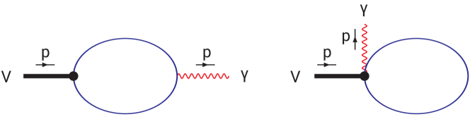
Figure 1: Diagrams describing the $V\to\gamma$ transition.

The relevant quark model diagrams of the $V\to\gamma$ transition are shown in Fig. 1. The corresponding Feynman one-loop integrals read

$$M^{\mu\nu}(p) =N_{c}g_{V}\!\int\!\!\frac{d^{4}k}{(2\pi)^{4}i}\Big{\{}\Phi_{V}(-k^{2})\,\text{tr}\Big{[}\gamma^{\mu}S(k+\tfrac{1}{2}\,p)\gamma^{\nu}S(k-\tfrac{1}{2}\,p)\Big{]}$$

$$\quad-\,\int\limits_{0}^{1}d\tau\Phi^{\prime}_{V}(-z_{\tau})(2\,k+\tfrac{1}{2}\,p)^{\mu}\text{tr}\Big{[}\gamma^{\nu}S(k)\Big{]}\Big{\}},$$ (3)

$$z_{\tau} =\tau(k+\tfrac{1}{2}\,p)^{2}+(1-\tau)k^{2}\,.$$

Here $N_{c}=3$ is the number of colors, $g_{V}$ is the coupling of the vector meson with its constituent quarks, $S$ denotes the quark propagator and $\Phi^{\prime}_{V}$ is the derivative of the vertex function with respect to its argument. In this paper we consider the charmonium ($c\bar{c}$-state) and bottomonium ($b\bar{b}$-state). The constituent quark propagator is written as

$$S(k)=\frac{1}{m_{q}-\not\!k},$$

where $m_{q}$ is the constituent quark mass. We use the Lorentz index $\mu$ in relation to the photon field whereas $\nu$ corresponds to the vector meson field. With the simple Gaussian form for the vertex function one has

$$\Phi_{V}(-k^{2})=\exp(s\,k^{2}),\quad\Phi^{\prime}_{V}(-k^{2})=-s\exp(s\,k^{2}),\quad\text{where}\quad s=1/\Lambda_{V}^{2}\,.$$ (4)

Here the parameter $\Lambda_{V}$ characterizes the size of the vector meson. One is allowed to use different choices for $\Phi_{V}$ as long as it falls off sufficiently fast in the ultraviolet region of Euclidean space to render the Feynman diagrams ultraviolet finite [37].

2.3 Gauge invariance

As the first step in our study, let us prove that the amplitude $M^{\mu\nu}$ given by Eq. (3) is gauge invariant, i.e. $M^{\mu\nu}p_{\mu}=0$. The loop (or bubble) integral contracted with $p_{\mu}$ can be written as

$$\int\!\!\frac{d^{4}k}{(2\pi)^{4}i}\Phi_{V}\left(-k^{2}\right)\,\text{tr}\Big{[}\!\not\!p\,S(k+\tfrac{1}{2}\,p)\gamma^{\nu}S(k-\tfrac{1}{2}\,p)\Big{]}$$

$$\quad=\int\!\!\frac{d^{4}k}{(2\pi)^{4}i}\Phi_{V}\left(-k^{2}\right)\,\Big{\{}\text{tr}\Big{[}S(k+\tfrac{1}{2}\,p)\gamma^{\nu}\Big{]}-\text{tr}\Big{[}S(k-\tfrac{1}{2}\,p)\gamma^{\nu}\Big{]}\Big{\}}\,.$$ (5)

The integrand of the tadpole integral contracted with $p_{\mu}$ may be transformed in the following way

$$-\int\limits_{0}^{1}d\tau\Phi^{\prime}_{V}\Big{(}-\tau(k+\tfrac{1}{2}\,p)^{2}-(1-\tau)k^{2}\Big{)}\left(2\,kp+\tfrac{1}{2}\,p^{2}\right)\text{tr}\Big{[}\gamma^{\nu}S(k)\Big{]}\Big{\}}$$

$$\quad=-\frac{\Phi_{V}\Big{(}-(k+\tfrac{1}{2}\,p)^{2}\Big{)}-\Phi_{V}\Big{(}-k^{2}\Big{)}}{k^{2}-(k+\tfrac{1}{2}p)^{2}}\,2\,\left(kp+\tfrac{1}{4}\,p^{2}\right)\text{tr}\Big{[}\gamma^{\nu}S(k)\Big{]}$$

$$\quad=2\,\Big{[}\Phi_{V}\Big{(}-(k+\tfrac{1}{2}\,p)^{2}\Big{)}-\Phi_{V}\Big{(}-k^{2}\Big{)}\Big{]}\text{tr}\Big{[}\gamma^{\nu}S(k)\Big{]}\,.$$

Finally, we use the identity

$$\int d^{4}kf(k)\text{tr}\Big{[}\gamma^{\nu}S(k)\Big{]}=\frac{1}{2}\int d^{4}k\left(f(k)-f(-k)\right)\text{tr}\Big{[}\gamma^{\nu}S(k)\Big{]},$$

which is valid for any well behaved function $f(k)$. We come to the final expression for the tadpole integral contracted with the external momentum $p$. One has

$$-\int\!\!\frac{d^{4}k}{(2\pi)^{4}i}\int\limits_{0}^{1}d\tau\Phi^{\prime}_{V}\Big{(}-\tau(k+\tfrac{1}{2}\,p)^{2}-(1-\tau)k^{2}\Big{)}\left(2\,kp+\tfrac{1}{2}\,p^{2}\right)\text{tr}\Big{[}\gamma^{\nu}S(k)\Big{]}$$

$$\quad=\int\!\!\frac{d^{4}k}{(2\pi)^{4}i}\Big{[}\Phi_{V}\Big{(}-(k+\tfrac{1}{2}\,p)^{2}\Big{)}-\Phi_{V}\Big{(}-(k-\tfrac{1}{2}\,p)^{2}\Big{)}\Big{]}\text{tr}\Big{[}\gamma^{\nu}S(k)\Big{]}$$

$$\quad=-\int\!\!\frac{d^{4}k}{(2\pi)^{4}i}\Phi_{V}\left(-k^{2}\right)\,\Big{\{}\text{tr}\Big{[}S(k+\tfrac{1}{2}\,p)\gamma^{\nu}\Big{]}-\text{tr}\Big{[}S(k-\tfrac{1}{2}\,p)\gamma^{\nu}\Big{]}\Big{\}}\,.$$ (6)

It is readily seen that the expression given by Eq. (5) is exactly canceled out by the one given in Eq. (6). Thus, we have $M^{\mu\nu}p_{\mu}=0$. It is interesting to see what is going on in the case of a null momentum $p=0$. If $p=0$ then the integral corresponding to the tadpole diagram may be transferred to the one corresponding to the loop diagram by using the integration by parts. One has

$$\int\frac{d^{4}k}{(2\pi)^{4}i}\,\Big{\{}\Phi_{V}\left(-k^{2}\right)\text{tr}\Big{[}\gamma^{\mu}S(k)\gamma^{\nu}S(k)\Big{]}-2k^{\mu}\,\Phi^{\prime}_{V}\left(-k^{2}\right)\text{tr}\Big{[}\gamma^{\nu}S(k)\Big{]}\Big{\}}$$

$$\quad=\int\frac{d^{4}k}{(2\pi)^{4}i}\,\frac{\partial}{\partial k^{\mu}}\Big{\{}\Phi_{V}\left(-k^{2}\right)\text{tr}\Big{[}\gamma^{\nu}S(k)\Big{]}\Big{\}}=0.$$ (7)

In the general case the invariant amplitude of the $V\to\gamma$ transition is written as

$$M^{\mu\nu}(p)=G_{V}(p^{2})\,g^{\mu\nu}+F_{V}(p^{2})\,p^{\mu}p^{\nu},$$

where the form factor $G_{V}$ has a dimension of mass squared whereas the form factor $F_{V}$ is dimensionless. The gauge invariance gives the relation between the two form factors

$$G_{V}(p^{2})=-p^{2}F_{V}(p^{2})$$ (8)

valid for any $p^{2}$ value. From Eq. (7) follows that both form factors do not have singularity at $p^{2}=0$. In the case of decay $V\to\ell^{+}\ell^{-}$, only the first form factor $G_{V}$ gives a contribution to the decay amplitude due to the conservation of the vector lepton current.

2.4 Results

By using the standard technique of integration over the loop momentum k one can finalize the two-fold integrals in the expressions for $V\to\gamma$ form factors. One can obtain the following expressions for the integrals from the loop diagram

$$G_{V}^{{\rm\,loop}}(p^{2})=$$

$$\qquad\frac{3g_{V}}{(4\pi)^{2}}\!\int\limits_{0}^{\infty}\!\frac{dt\,t}{(s+t)^{2}}\int\limits_{0}^{1}\!d\alpha\,e^{z_{\alpha}}\Big{\{}4\,m_{q}^{2}+\frac{4}{s+t}+\Big{[}1-\frac{4\,t^{2}}{(s+t)^{2}}\left(\tfrac{1}{2}-\alpha\right)^{2}\Big{]}p^{2}\Big{\}},$$

$$F_{V}^{{\rm\,loop}}(p^{2})=$$

$$\qquad\frac{3g_{V}}{(4\pi)^{2}}\!\int\limits_{0}^{\infty}\!\frac{dt\,t}{(s+t)^{2}}\int\limits_{0}^{1}\!d\alpha\,e^{z_{\alpha}}\Big{\{}-2+\frac{8\,t^{2}}{(s+t)^{2}}\left(\tfrac{1}{2}-\alpha\right)^{2}\Big{\}},$$

$$z_{\alpha}=-t\left[m_{q}^{2}-\alpha(1-\alpha)\,p^{2}\right]+\frac{st}{s+t}\left(\tfrac{1}{2}-\alpha\right)^{2}p^{2}.$$

In the case of the tadpole diagram, one has

$$G_{V}^{{\rm\,tad}}(p^{2}) =\frac{3g_{V}}{(4\pi)^{2}}\!\int\limits_{0}^{\infty}\!\frac{dt\,s}{(s+t)^{2}}\int\limits_{0}^{1}\!d\tau\,e^{z_{\tau}}\Big{[}-\frac{4}{s+t}\Big{]},$$

$$F_{V}^{{\rm\,tad}}(p^{2}) =\frac{3g_{V}}{(4\pi)^{2}}\!\int\limits_{0}^{\infty}\!\frac{dt\,s}{(s+t)^{2}}\int\limits_{0}^{1}\!d\tau\,e^{z_{\tau}}\Big{[}-\Big{(}1-\frac{2s\tau}{s+t}\Big{)}\frac{s\tau}{s+t}\Big{]},$$

$$z_{\tau} =-tm_{q}^{2}+s\tau\left(1-\frac{s\tau}{s+t}\right)\frac{p^{2}}{4}.$$

Then we define the full $V\to\gamma$ form factors as

$$G_{V}(p^{2}) =G_{V}^{{\rm\,loop}}(p^{2})+G_{V}^{{\rm\,tad}}(p^{2})\,,$$

$$F_{V}(p^{2}) =F_{V}^{{\rm\,loop}}(p^{2})+F_{V}^{{\rm\,tad}}(p^{2})\,.$$

Their numerical values are calculated by using the FORTRAN codes which require the NAG library.

The model parameters were determined by fitting calculated quantities of basic processes to available experimental data or lattice simulations (for details, see Ref. [31]). Here, we take the values of the constituent quark masses $m_{q}$ from an updated fit made in [38]. This fit improves the description of new data on the exclusive $B$-meson and heavy baryon decays. Note that in the fit, the infrared cutoff parameter $\lambda$ has been kept fixed. The updated numerical values of the constituent quark masses and the cutoff parameter $\lambda$ are given in Table 1.

$m_{u}$	$m_{s}$	$m_{c}$	$m_{b}$	$\lambda$
$0.241$	$0.428$	$1.67$	$5.04$	$0.181$	GeV

Table 1: Model parameters: quark masses and cutoff parameter $\lambda$ (all in GeV).

Size parameters of charmonium and bottomonium are

$$\Lambda_{J/\psi}=2.795(1)~{}{\rm GeV},\qquad\Lambda_{\Upsilon}=4.03(4)~{}{\rm GeV}.$$

The masses of ground and radially excited states of charmonium and bottomonium are given in Table 2.

$J/\Psi$	$\Psi(2s)$		$\Upsilon(1s)$	$\Upsilon(2s)$	$\Upsilon(3s)$
$3096.900(6)$	$3686.10(6)$		$9460.30(26)$	$10023.26(31)$	$10355.2(5)$

Table 2: Masses of charmonia and bottomonia from PDG [39] (in MeV).

First, we have checked numerically that the equation (8) is satisfied with high accuracy (6 digits calculated with relative error $10^{-5}$). The term proportional to $p^{\mu}$ does not contribute to the amplitude of the $V\to\gamma\to\ell^{-}\ell^{+}$ decay due to the conservation of the lepton current. Therefore we will use the form factor $G_{V}(p^{2})=-p^{2}F_{V}(p^{2})$ on the mass shell of the vector meson $p^{2}=m_{V}^{2}$ for the calculation of the decay width. One has

$$\Gamma(V\to\ell^{+}\ell^{-})=\frac{4\pi\alpha^{2}}{3}\,m_{V}\Big{(}\frac{Q_{V}f_{V}}{m_{V}}\Big{)}^{2}\sqrt{1-4x_{\ell}^{2}}\,(1+2x_{\ell}^{2}),$$

where $f_{V}\equiv G_{V}(m_{V}^{2})/m_{V}$, $x_{\ell}=m_{\ell}/m_{V}$ and the quark charge factor $Q_{V}=(e_{u}-e_{d})/\sqrt{2}=1/\sqrt{2}$ for the $\rho^{0}$ meson, $Q_{V}=e_{c}=2/3$ for $\psi$ mesons, and $Q_{V}=e_{b}=-1/3$ for $\Upsilon$ mesons. Note that in our notation the leptonic constant $f_{V}$ coincides with the weak leptonic constant and has the dimension of mass. The results as predicted by the CCQM are summarized in Table 3. The theoretical errors correspond to the propagated errors of hadronic parameters $\Lambda_{V}$, which, on their turn, get the error from the fit of the CCQM to decay width experimental data.

Quantity	$J/\psi$		$\Upsilon(1s)$
$f_{V}$ (MeV)	415.4		715
	CCQM	Expt.	CCQM	Expt.
$B(V\to\tau^{+}\tau^{-})$ (%)			$2.46(7)$	$2.60(10)$
$B(V\to\mu^{+}\mu^{-})$ (%)	$5.964(40)$	$5.961(33)$	$2.48(7)$	$2.48(5)$
$B(V\to e^{+}e^{-})$ (%)	$5.964(40)$	$5.971(32)$	$2.48(7)$	$2.38(11)$

Table 3: Leptonic branching fractions of $J/\psi$ and $\Upsilon(1s)$ compared to experimental numbers.

3 New approach to radial excitations

3.1 First step: running quark mass in a loop

We assume that the binding energy of the radial excitations of a quarkonium $q\bar{q}$ is equal to the binding energy $E$ of the ground state $V_{0}$: $E=m_{V_{0}}-2m_{q_{0}}$. This means that the value of the constituent quark mass is for an excited state $V^{\prime}$ equal to

$$m_{q^{\prime}}=(m_{V^{\prime}}-E)/2.$$ (9)

The ground state quark masses are taken from Table 1. We find the values of the size parameters $\Lambda_{V}$ by fitting the model to the experimental data on the leptonic decays $V\to\ell^{+}\ell^{-}$. The size parameters and branching fractions predicted under this assumption are shown in Tabs. 4 and 5.

	$J/\psi$		$\Psi(2s)$
$\Lambda_{V}$(GeV)	2.795		1.68
	CCQM	Expt.	CCQM	Expt.
$\mathcal{B}(V\to\tau^{+}\tau^{-})$(%)	-		0.31(1)	0.31(4)
$\mathcal{B}(V\to\mu^{+}\mu^{-})$(%)	5.964(40)	5.961(33)	0.80(2)	0.80(6)
$\mathcal{B}(V\to e^{+}e^{-})$(%)	5.964(40)	5.971(32)	0.80(2)	0.79(2)

Table 4: Charmonia: size parameters and leptonic branching fractions with running constituent quark masses.

	$\Upsilon(1s)$		$\Upsilon(2s)$		$\Upsilon(3s)$
$\Lambda_{V}$(GeV)	4.03		2.80		2.485
	CCQM	Expt.	CCQM	Expt.	CCQM	Expt.
$\mathcal{B}(V\to\tau^{+}\tau^{-})$(%)	2.46(7)	2.60(10)	1.90(0.5)	2.00(21)	2.17(3)	2.29(30)
$\mathcal{B}(V\to\mu^{+}\mu^{-})$(%)	2.48(7)	2.48(5)	1.92(0.5)	1.93(17)	2.18(3)	2.18(21)
$\mathcal{B}(V\to e^{+}e^{-})$(%)	2.48(7)	2.38(11)	1.92(0.5)	1.91(16)	2.18(3)	2.18(20)

Table 5: Bottomonia: size parameters and leptonic branching fractions with running constituent quark masses.

3.2 Second step: orthogonality of the radial excitations

We assume that different radial excitations cannot pass into each other through a quark loop. We call this assumption as the orthogonality condition. To realize this condition we choose the vertex functions in the following form

$$\Phi_{n}(-k^{2})=\Big{(}1+\sum\limits_{m=1}^{n}c_{m+n-1}s_{n}^{m}k^{2m}\Big{)}\Phi_{V}(-k^{2}),$$ (10)

where the function $\Phi_{V}(-k^{2})$ is given by Eq. (4). Then the orthogonality condition implies that

$$\left(g_{\mu\nu}-\frac{p_{\mu}p_{\nu}}{p^{2}}\right)\!\int\!\!\frac{d^{4}k}{(2\pi)^{4}i}\Phi_{n}(-k^{2})\,\Phi_{m}(-k^{2})\text{tr}\Big{[}\gamma^{\mu}S(k+\tfrac{1}{2}\,p)\gamma^{\nu}S(k-\tfrac{1}{2}\,p)\Big{]}=0.$$ (11)

This condition will allow us to determine the numerical values of the coefficients $c_{m+n-1}$ in the allowed region of $p^{2}$ for certain quarkonium spectrum. Here, we consider two radial excitations of the charmonium, $J/\psi$ and $\Psi(2S)$, and three for the bottomonium: $\Upsilon(1S)$, $\Upsilon(2S)$ and $\Upsilon(3S)$. We find the values of coefficients $c_{i}$ which solve (11) for charmonia and bottomonia separately, the solution depends on the quarkonium mass. This dependence is shown in Fig. 2.

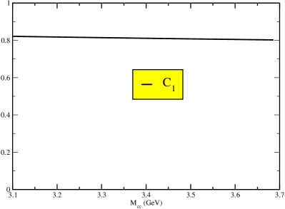
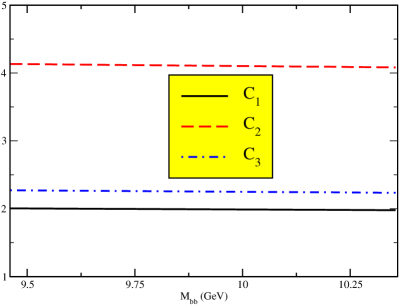
Figure 2: The dependence of coefficients of the orthogonal vertex functions on the quarkonium mass for charmonia and bottomonia.

3.3 Results and discussion

	$J/\psi$		$\Psi(2s)$
$\Lambda_{V}$(GeV)	2.795		0.463
$c_{i}$			$c_{1}=0.802$
	CCQM	Expt.	CCQM	Expt.
$\mathcal{B}(V\to\tau^{+}\tau^{-})$(%)	-		0.31(1)	0.31(4)
$\mathcal{B}(V\to\mu^{+}\mu^{-})$(%)	5.964(40)	5.961(33)	0.81(2)	0.80(6)
$\mathcal{B}(V\to e^{+}e^{-})$(%)	5.964(40)	5.971(32)	0.81(2)	0.79(2)

Table 6: Charmonia: size parameters and leptonic branching fractions in the new approach with running constituent quark masses and orthogonal vertex functions.

	$\Upsilon(1s)$		$\Upsilon(2s)$		$\Upsilon(3s)$
$\Lambda_{V}$(GeV)	4.03		3.77		3.01
$c_{i}$		$c_{1}=1.979,\;c_{2}=4.083,\;c_{3}=2.235$
	CCQM	Expt.	CCQM	Expt.	CCQM	Expt.
$\mathcal{B}(V\to\tau^{+}\tau^{-})$(%)	2.46(7)	2.60(10)	1.92(0.5)	2.00(21)	2.17(3)	2.29(30)
$\mathcal{B}(V\to\mu^{+}\mu^{-})$(%)	2.48(7)	2.48(5)	1.93(0.5)	1.93(17)	2.18(3)	2.18(21)
$\mathcal{B}(V\to e^{+}e^{-})$(%)	2.48(7)	2.38(11)	1.93(0.5)	1.91(16)	2.18(3)	2.18(20)

Table 7: Bottomonia: size parameters and leptonic branching fractions in the new approach with running constituent quark masses and orthogonal vertex functions.

With quark masses defined by (9) and modified vertex functions (10), where the coefficients are determined by (11), we settle, in an optimization procedure, the value of size parameters $\Lambda_{V}$ so as to get the best description of leptonic decay widths. We then get our results summarized in Tabs. 6 and 7. The difference between the theory and the experimental values is, in terms of standard deviations, shown in Table 8.

	$\left|\mathcal{B}_{\text{expt}}-\mathcal{B}_{\text{CCQM}}\right|/\sigma\left(\mathcal{B}_{\text{expt}}-\mathcal{B}_{\text{CCQM}}\right)$
	$J/\psi$	$\Psi(2s)$		$\Upsilon(1s)$	$\Upsilon(2s)$	$\Upsilon(3s)$
$\tau^{+}\tau^{-}$		$\ll$1		1.15	0.38	0.40
$\mu^{+}\mu^{-}$	0.06	0.16		$\ll$1	$\ll$1	$\ll$1
$e^{+}e^{-}$	0.12	0.71		0.77	0.12	$\ll$1

Table 8: The difference between CCQM values and the experiment expressed in terms of standard deviations.

As readily seen, only one difference slightly exceeds $1\sigma$ deviation, others are within the $1\sigma$ interval. In this sense we are able to describe the experimental measurements within our CCQM SM approach. Taking into the account the relation with the semileptonic decays mentioned in the Introduction, our results do not give support for new physics phenomena being involved in the latter.

On the other hand, the results presented in Tabs. 6 and 7 were reached as fits where parameters were tuned and not as predictions. This is natural, since we are presenting here a novel approach where the orthogonal vertex functions were presented for the first time with their parameters not settled until now. It is certainly desirable to analyze other processes in future, where heavy quarkonia or possible other particles with their excited states play a role. This will ensure that the number of parameters is significantly smaller than the number of observables, i.e. the model will become more constrained with more predictive power. Additionally, as part of our outlook, the CCQM can be extended to include new physics EFT operators, similarly to what has been presented in [23]. Then the corresponding Wilson coefficients can be analyzed for semileptonic and leptonic decays and conclusions about their significance drawn from the comparison to data.

References

- [1] Johann H. Kuhn, A. A. Penin, A. A. Pivovarov. Coulomb resummation for b anti-b system near threshold and precision determination of alpha(s) and m(b). Nucl. Phys. B, 534:356–370, 1998.
- [2] Clara Peset, Antonio Pineda, Jorge Segovia. The charm/bottom quark mass from heavy quarkonium at N3LO. JHEP, 09:167, 2018.
- [3] J. Resag, C. R. Munz. Heavy quarkonia in the instantaneous Bethe-Salpeter model. Nucl. Phys. A, 590:735, 1995.
- [4] Stephan Narison. QCD parameter correlations from heavy quarkonia. Int. J. Mod. Phys. A, 33(10):1850045, 2018. [Addendum: Int.J.Mod.Phys.A 33, 1892004 (2018)].
- [5] N. Brambilla, i in. Heavy quarkonium physics. 12 2004.
- [6] N. Brambilla, i in. Heavy Quarkonium: Progress, Puzzles, and Opportunities. Eur. Phys. J. C, 71:1534, 2011.
- [7] Alexander Rothkopf. Heavy Quarkonium in Extreme Conditions. Phys. Rept., 858:1–117, 2020.
- [8] J. P. Lees, i in. Evidence for an excess of decays. Phys. Rev. Lett., 109:101802, 2012.
- [9] Roel Aaij, i in. Test of lepton universality using decays. Phys. Rev. Lett., 113:151601, 2014.
- [10] Roel Aaij, i in. Measurement of the ratios of branching fractions and . Phys. Rev. Lett., 131:111802, 2023.
- [11] R. Aaij, i in. Measurement of lepton universality parameters in and decays. Phys. Rev. D, 108(3):032002, 2023.
- [12] Roel Aaij, i in. Test of lepton flavor universality using decays with hadronic channels. Phys. Rev. D, 108(1):012018, 2023.
- [13] G. Caria, i in. Measurement of and with a semileptonic tagging method. Phys. Rev. Lett., 124(16):161803, 2020.
- [14] Roel Aaij, i in. Test of lepton universality in beauty-quark decays. Nature Phys., 18(3):277–282, 2022. [Addendum: Nature Phys. 19, (2023)].
- [15] Darius A. Faroughy, Admir Greljo, Jernej F. Kamenik. Confronting lepton flavor universality violation in B decays with high- tau lepton searches at LHC. Phys. Lett. B, 764:126–134, 2017.
- [16] R. Van Royen, V. F. Weisskopf. Hadron Decay Processes and the Quark Model. Nuovo Cim. A, 50:617–645, 1967. [Erratum: Nuovo Cim.A 51, 583 (1967)].
- [17] Estia J. Eichten, Chris Quigg. Quarkonium wave functions at the origin. Phys. Rev. D, 52:1726–1728, 1995.
- [18] Miguel Angel Sanchis-Lozano. Leptonic universality breaking in upsilon decays as a probe of new physics. Int. J. Mod. Phys. A, 19:2183, 2004.
- [19] Stanley F. Radford, Wayne W. Repko. Potential model calculations and predictions for heavy quarkonium. Phys. Rev. D, 75:074031, 2007.
- [20] Ajay Kumar Rai, Bhavin Patel, P. C. Vinodkumar. Properties of mesons in non-relativistic QCD formalism. Phys. Rev. C, 78:055202, 2008.
- [21] Manan Shah, Arpit Parmar, P. C. Vinodkumar. Leptonic and Digamma decay Properties of S-wave quarkonia states. Phys. Rev. D, 86:034015, 2012.
- [22] M. B. Voloshin. Charmonium. Prog. Part. Nucl. Phys., 61:455–511, 2008.
- [23] Daniel Aloni, Aielet Efrati, Yuval Grossman, Yosef Nir. and leptonic decays as probes of solutions to the puzzle. JHEP, 06:019, 2017.
- [24] Guo-Li Wang, Xing-Gang Wu. Revisiting the Heavy Vector Quarkonium Leptonic Widths. Chin. Phys. C, 44(6):063104, 2020.
- [25] M. Beneke, A. Signer, Vladimir A. Smirnov. Two loop correction to the leptonic decay of quarkonium. Phys. Rev. Lett., 80:2535–2538, 1998.
- [26] Martin Beneke, Yuichiro Kiyo, Peter Marquard, Alexander Penin, Jan Piclum, Dirk Seidel, Matthias Steinhauser. Leptonic decay of the (1) meson at third order in QCD. Phys. Rev. Lett., 112(15):151801, 2014.
- [27] Feng Feng, Yu Jia, Zhewen Mo, Jichen Pan, Wen-Long Sang, Jia-Yue Zhang. Complete three-loop QCD corrections to leptonic width of vector quarkonium. 7 2022.
- [28] A. Gray, I. Allison, C. T. H. Davies, Emel Dalgic, G. P. Lepage, J. Shigemitsu, M. Wingate. The Upsilon spectrum and m(b) from full lattice QCD. Phys. Rev. D, 72:094507, 2005.
- [29] D. Hatton, C. T. H. Davies, B. Galloway, J. Koponen, G. P. Lepage, A. T. Lytle. Charmonium properties from lattice +QED : Hyperfine splitting, leptonic width, charm quark mass, and . Phys. Rev. D, 102(5):054511, 2020.
- [30] D. Hatton, C. T. H. Davies, J. Koponen, G. P. Lepage, A. T. Lytle. Bottomonium precision tests from full lattice QCD: Hyperfine splitting, leptonic width, and b quark contribution to hadrons. Phys. Rev. D, 103(5):054512, 2021.
- [31] Tanja Branz, Amand Faessler, Thomas Gutsche, Mikhail A. Ivanov, Jurgen G. Korner, Valery E. Lyubovitskij. Relativistic constituent quark model with infrared confinement. Phys. Rev. D, 81:034010, 2010.
- [32] Mikhail A. Ivanov, Jurgen G. Korner, Pietro Santorelli. Exclusive semileptonic and nonleptonic decays of the meson. Phys. Rev. D, 73:054024, 2006.
- [33] Gurjav Ganbold, Thomas Gutsche, Mikhail A. Ivanov, Valery E. Lyubovitskij. On the meson mass spectrum in the covariant confined quark model. J. Phys. G, 42(7):075002, 2015.
- [34] Stanislav Dubnička, Anna Z. Dubničková, Nurgul Habyl, Mikhail A. Ivanov, Andrej Liptaj, Guliya S. Nurbakova. Decay in covariant quark model. Few Body Syst., 57(2):121–143, 2016.
- [35] John Terning. Gauging nonlocal Lagrangians. Phys. Rev. D, 44(3):887–897, 1991.
- [36] Tanja Branz, Amand Faessler, Thomas Gutsche, Mikhail A. Ivanov, Jurgen G. Korner, Valery E. Lyubovitskij, Bettina Oexl. Radiative decays of double heavy baryons in a relativistic constituent three–quark model including hyperfine mixing. Phys. Rev. D, 81:114036, 2010.
- [37] I. V. Anikin, Mikhail A. Ivanov, N. B. Kulimanova, Valery E. Lyubovitskij. The Extended Nambu-Jona-Lasinio model with separable interaction: Low-energy pion physics and pion nucleon form-factor. Z. Phys. C, 65:681–690, 1995.
- [38] Thomas Gutsche, Mikhail A. Ivanov, Jürgen G. Körner, Valery E. Lyubovitskij, Pietro Santorelli, Nurgul Habyl. Semileptonic decay in the covariant confined quark model. Phys. Rev. D, 91(7):074001, 2015. [Erratum: Phys.Rev.D 91, 119907 (2015)].
- [39] R. L. Workman, i in. Review of Particle Physics. PTEP, 2022:083C01, 2022.