FULL-REFERENCE POINT CLOUD QUALITY ASSESSMENT
USING SPECTRAL GRAPH WAVELETS
Abstract
Point clouds in 3D applications frequently experience quality degradation during processing, e.g., scanning and compression. Reliable point cloud quality assessment (PCQA) is important for developing compression algorithms with good bitrate-quality trade-offs and techniques for quality improvement (e.g., denoising). This paper introduces a full-reference (FR) PCQA method utilizing spectral graph wavelets (SGWs). First, we propose novel SGW-based PCQA metrics that compare SGW coefficients of coordinate and color signals between reference and distorted point clouds. Second, we achieve accurate PCQA by integrating several conventional FR metrics and our SGW-based metrics using support vector regression. To our knowledge, this is the first study to introduce SGWs for PCQA. Experimental results demonstrate the proposed PCQA metric is more accurately correlated with subjective quality scores compared to conventional PCQA metrics.
Index Terms— point cloud quality assessment, full reference metric, graph signal processing, spectral graph wavelet, support vector regression
1 Introduction
Point clouds are a general 3D format representing realistic 3D objects in diverse 3D applications such as telepresence, monitoring, and holographic display. However, the perceptual quality of point clouds often deteriorates during scanning, compression, and transmission. Point cloud compression methods have been proposed to achieve a good trade-off between quality and bitrate. For instance, the MPEG committee has standardized two approaches: geometry-based point cloud compression (G-PCC) and video-based point cloud compression (V-PCC) [1]. Moreover, many methods aiming at improving point cloud quality have been proposed to mitigate the impact of distortions (e.g., point cloud denoising [2], upsampling [3], and inpainting [4]). Accurate point cloud quality assessment (PCQA) methods are essential to evaluate compression and quality enhancement methods.
Methods for PCQA can be classified into full-reference point cloud quality assessment (FR-PCQA) and no-reference point cloud quality assessment (NR-PCQA) approaches. Unlike NR-PCQA metrics [5, 6, 7], which cannot access a reference (noise-free) point cloud, FR-PCQA methods show reliable and stable assessment results when a good reference is available. For example, some of the FR-PCQA metrics [8, 9] have been utilized as criteria for evaluating point cloud compression methods in the MPEG standardization [1]. While these methods [8, 9] primarily focus on point-wise errors, alternative approaches that consider (i) more complex features (e.g., structural similarity [10, 11, 12] or (ii) graph similarity [13, 14]) have been proposed to improve the correlation with subjective assessment scores such as mean opinion score (MOS).
In recent years, learning-based FR-PCQA methods [15, 16, 17] have been shown to obtain better correlation with subjective assessment scores. Our previous study, full-reference quality assessment using support vector regression (FRSVR) [17], achieves high correlation with subjective assessment scores by integrating five different FR-PCQA metrics using support vector regression (SVR) and achieved first place in the FR broad-range quality estimation track in the ICIP 2023 point cloud visual quality assessment grand challenge (ICIP 2023 PCVQA grand challenge) [18]. Since it was designed for a grand challenge focused on PCQA for compression distortion only, FRSVR achieves less correlation with subjective assessment scores for other types of noise (e.g., Gaussian noise, down-sampling). In particular, the five types of scores adopted by FRSVR do not consider multi-scale features, which, according to previous studies [12, 14], are effective in assessing various types of distortion. Specifically, FRSVR utilizes two point-wise error metrics to evaluate geometric distortion but does not carry out region-to-region comparisons. Similarly, although region-to-region comparison is performed for color distortion, this is a single-scale feature calculated from a specified number of neighbors.
As an alternative, in this paper, we propose a more accurate FR-PCQA method using a spectral graph wavelet (SGW), which can provide multi-scale features as graph signal frequencies. In addition, the proposed method is faster than conventional multi-scale FR-PCQA methods [12, 14] because a fast calculation technique has been proposed for spectral graph wavelet transform (SGWT) s such as polynomial approximation [19].
Our contributions are as follows:
-
1.
we propose a novel spectral graph wavelet-based point cloud quality assessment (SGW-PCQA) metric that compares SGW s calculated from the coordinate and color signals of both reference and distorted point clouds. The previous studies on point cloud denoising based on SGW s [20, 21, 22] demonstrate that noise in geometric and color information can be eliminated by suppressing the high-frequency components of SGW s. Thus, comparing SGW s calculated from reference and distorted point clouds is useful to evaluate the amount of noise in the distorted point cloud. As far as we know, this is the first study to introduce SGW s for PCQA.
-
2.
To improve the correlation coefficients with subjective assessment scores, we use SVR to integrate the SGW-PCQA metrics with two out of the five metrics introduced in our previous SVR-based method, FRSVR [17]. This integrated version, SGW-PCQA +, leads to better correlation coefficients for both compression distortion and other types of distortions, such as Gaussian noise and downsampling. In addition, SGW-PCQA + outperformed the results of our previous work (FRSVR [17]) recorded in the ICIP 2023 PCVQA grand challenge in terms of the correlation coefficients with MOS and processing time.
2 Related work
Since this paper focuses on FR-PCQA, we introduce conventional FR-PCQA methods in this section.
2.1 3D-to-2D projection-based methods
Conventional image quality assessment techniques can be used to assess the quality of 3D point clouds by projecting them into multiple 2D planes. In [23], multiple projected 2D images are assessed by popular 2D image quality assessment metrics (e.g., VIFP [24], SSIM [25]). An attention-guided PCQA inspired by the structural similarity measure of [26] has also been proposed [27]. However, these methods suffer from a low correlation with subjective assessment scores since there is a loss of 3D information during projection.
2.2 3D model-based methods
Geometric distortions, e.g., point-to-point error [8], point-to-plane error [9] and plane-to-plane error [28], have also been introduced, but they cannot evaluate color distortion, so their applicability for PCQA is limited.
To evaluate color distortion, the Peak Signal-to-Noise Ratio (PSNR) [8] and PointSSIM [10] have been proposed. However, their correlation with subjective assessment scores is still limited since these methods compare only one feature (e.g., color [8] or local color variance [10]). To improve the reliability of PCQA metrics, point cloud quality metric (PCQM) [11] introduces a weighted linear combination of geometric and color distortions. Graph-based FR-PCQA distortions methods[13] and multi-scale methods have also been proposed to further improve the accuracy [12, 14]. However, the improved accuracy of [11, 12, 13, 14] comes with a large increase in computational complexity.
2.3 Learning-based methods
Recently, learning-based techniques have been introduced to obtain better correlation with subjective assessment scores. Unlike previously mentioned approaches, these methods require training a model using subjective assessment scores such as MOS. Examples of these approaches include [15], an end-to-end deep-learning framework for accurate FR-PCQA and [16], a learning-based method utilizing various PCA-based features. While [15, 16] demonstrate a high correlation with subjective assessment scores and combine geometry and color information, they suffer from large processing time for prediction. By using the SVR-based method [17] to combine simple FR-PCQA metrics by SVR, we achieve high correlation with subjective assessment scores for compression distortion with relatively low complexity. However, this approach is less reliable for other types of noises (e.g., Gaussian noise, down-sampling), as discussed in Section 1.
3 Preliminaries
3.1 Graph and point cloud notations
We begin by introducing mathematical notations and definitions relevant to graphs. An undirected and weighted graph is constructed with a point cloud , where and denote the set of nodes and edges on a graph, respectively. In this paper, a point cloud is characterized by the coordinate signals and color (lightness) signals . As in [11], we represent color using lightness in the LAB color space [29].
The adjacency matrix of the graph corresponding to a point cloud defines the edge weights between nodes (points) and using the Gaussian kernel function as:
| (1) |
where shows the coordinate signals at point and denotes the average of all pairwise distances. We have that if is one of the neighbors of . The definition of neighbors is determined and parameterized by a graph construction algorithm (e.g., K nearest neighbors (KNN)).
The combinatorial graph Laplacian is computed by , where is the degree matrix of [30]. characterizes the global smoothness of a graph signal because the graph Laplacian quadratic form is derived from where the sum is over all pairs of connected nodes and , denoted by . The graph Fourier transform is defined as , where and denote the -th eigenvalue and eigenvector of , respectively.
3.2 Spectral graph wavelet transform (SGWT)
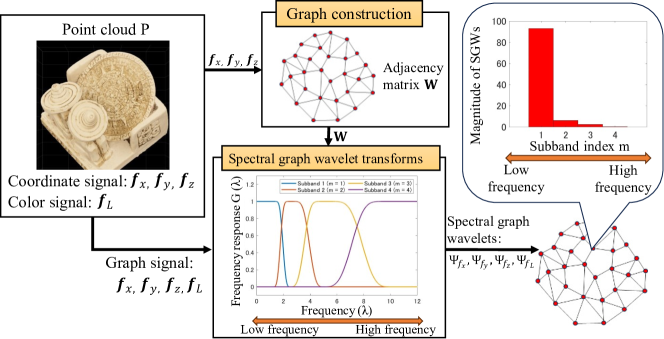
Fig. 1 illustrates the calculation process of SGWT [19, 31] for a point cloud . SGWT s are constructed using a kernel operator , which acts on a graph signal by modulating each graph Fourier mode: . A scaled operator shows the scaling in the spectral domain at scale , where is the index of the band-pass filter, as shown in Fig. 1. At this time, the wavelets are calculated by applying to a single vertex operator: where is the impulse on vertex . Then, the SGW coefficients , where indicates the number of band-pass filters, are calculated by
| (2) |
4 Proposed method
4.1 Overview of the proposed method
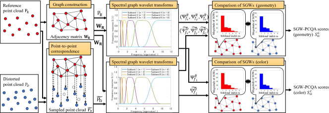
Reference and distorted point clouds are represented as and , respectively, where denotes the number of points of . Point clouds and have three coordinate signals and one color signal and , respectively. Fig. 2 shows the overall calculation flow of the proposed method called SGW-PCQA, which includes the following five steps.
-
1.
A graph with adjacency matrix is constructed from by KNN.
-
2.
Point-to-point correspondence between and is calculated. The nearest point in from is selected as by the nearest neighbor search using Euclidean distance. The associated distorted point cloud has the signals .
-
3.
The SGW coefficients with graph are calculated for each graph signal , , , , , , and . The resulting SGW coefficients are , ,, , , , and .
-
4.
The geometry PCQA score and color PCQA score are computed by comparing the SGW coefficients at the -th subband.
-
5.
A trained SVR model predicts a final assessment score from the scores and . Note that the parameters of the SVR model are optimized using a training set, including the scores calculated in step 4 and the MOS of the corresponding distorted point clouds.
We explain steps 1, 2, and 3 in Section 4.2. Steps 4 and 5 are described in Section 4.3 and Section 4.4, respectively. Furthermore, SGW-PCQA +, which is an extension of SGW-PCQA, is described in Section 4.5.
4.2 Calculation of spectral graph wavelets
This section explains how to calculate SGWs for PCQA. In graph signal processing, the definition of graph frequency depends on the structure of the graph [30]. Hence, if graphs are independently constructed from reference and distorted point clouds, the definitions of their respective graph frequencies will be different. Therefore, to perform PCQA, if we wish to compare the graph frequencies obtained from and , we first must select a common graph for the two point clouds.
In the proposed method, a graph with the adjacency matrix is calculated from the reference point cloud by KNN, using (1). Then, the nearest point from a query point is extracted by the nearest neighbor search based on the 3D Euclidean distance to project into . In this way, we obtain a new distorted point cloud that has the same node indices but different graph signals. Finally, the SGW coefficients are calculated from coordinate and color signals of and based on (2). Since SGWT s are computed for each graph signal ( and ), SGWT coefficients (, and ) are output.
4.3 SGW-based FR-PCQA metrics
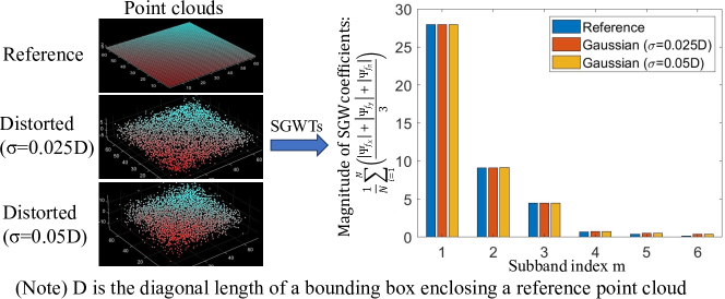
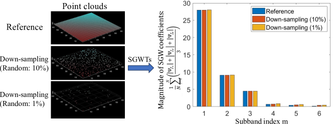
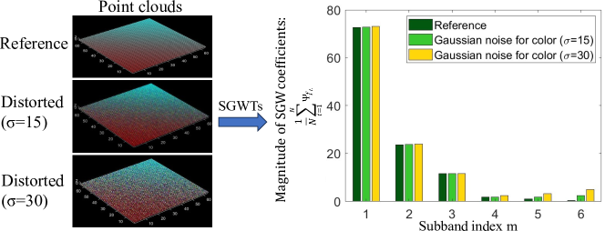
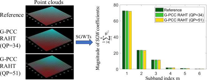
Fig. 3 shows the results of our preliminary experiment, which confirmed that SGWs change under several types of distortions. As shown in Fig. 3, since SGW s at various subbands are changed when distortions are introduced, the quality can be assessed by observing the changes of SGW s.
In the proposed SGW-PCQA method, to assess geometric distortion, the differences in SGWs of , and coordinates for each -th subband are calculated as follows:
| (3) |
| (4) |
| (5) |
| (6) |
Geometric assessment scores are calculated as
| (7) |
Likewise, color assessment scores are given as
| (8) |
| (9) |
4.4 Score integration by support vector regression (SVR)
We use SVR to predict a final PCQA score. Multiple scores, and , are integrated by SVR. During the training phase, an SVR model is trained using the MOS of the corresponding distorted point clouds and the multiple PCQA scores calculated from training data. The Gaussian radial basis function (RBF) kernel and the sequential minimal optimization [32] are chosen as a kernel and solver of SVR, respectively.
4.5 Extension of SGW-PCQA (SGW-PCQA +)
In our preliminary experiments, the performance of SGW-PCQA can be further improved by adding some of the FR-PCQA scores utilized in our previous work, FRSVR [17]. Thus, we selected two types of scores utilized in FRSVR, (1) point-to-point score () and (2) graph total variation (GTV)-based score (), whose addition significantly improved the correlation with subjective scores. The point-to-point score is based on point-to-point error [8]. The GTV-based score is calculated by comparing GTV s, which quantify the smoothness of graph signals (Please see [17] to access the detailed formulas due to space limitation).
Although SGW s reflect graph signal variation at various scales, they cannot consider too local and global information. Since the point-to-point and GTV-based scores focus on very local (point-wise) and global information, respectively, adding these scores leads to improved correlation with subjective scores. In addition, although graph construction is required to calculate these two scores, a graph utilized for calculating SGW s can be reused. Thus, the additional processing time is not very large. The extension that combines these two scores ( and ) with the SGW-based scores ( and ) using SVR is named as SGW-PCQA +.
5 EXPERIMENTS
| # | Geometry score set | Color score set | BASICS [33] | WPC [34] | Average | |||
| PLCC | SROCC | PLCC | SROCC | PLCC | SROCC | |||
| #1 | 0.844 | 0.770 | 0.787 | 0.780 | 0.816 | 0.775 | ||
| #2 | , | , | 0.880 | 0.815 | 0.835 | 0.815 | 0.858 | 0.815 |
| #3 | , , | , , | 0.874 | 0.837 | 0.854 | 0.842 | 0.864 | 0.840 |
| #4 | , , , | , , , | 0.870 | 0.837 | 0.863 | 0.854 | 0.867 | 0.846 |
| #5 | , , , , | , , , , | 0.875 | 0.835 | 0.847 | 0.834 | 0.861 | 0.835 |
| #6 | , , , , , | , , , , , | 0.889 | 0.843 | 0.826 | 0.814 | 0.858 | 0.829 |
| #7 | , , , , , | , , | 0.892 | 0.861 | 0.845 | 0.840 | 0.869 | 0.851 |
| #8 | , , , , , | , , , | 0.888 | 0.859 | 0.842 | 0.837 | 0.865 | 0.848 |
| #9 | , , , , , | , , , , | 0.879 | 0.835 | 0.828 | 0.823 | 0.854 | 0.829 |
| Metric | BASICS [33] | WPC [34] | Average | ||||||
|---|---|---|---|---|---|---|---|---|---|
| PLCC | SROCC | Time [s] | PLCC | SROCC | Time [s] | PLCC | SROCC | Time [s] | |
| Point-to-point (MSE) [8] | 0.041 | 0.735 | 9.701 | 0.401 | 0.566 | 6.832 | 0.221 | 0.651 | 8.267 |
| Point-to-plane (MSE) [8] | 0.005 | 0.799 | 49.122 | 0.368 | 0.481 | 32.847 | 0.187 | 0.640 | 40.985 |
| Angular similarity [28] | 0.328 | 0.306 | 39.155 | 0.296 | 0.319 | 27.336 | 0.312 | 0.313 | 33.246 |
| Y-MSE [8] | 0.512 | 0.550 | 9.896 | 0.469 | 0.591 | 6.928 | 0.491 | 0.571 | 8.412 |
| PointSSIM [10] | 0.605 | 0.620 | 23.682 | 0.469 | 0.471 | 15.281 | 0.537 | 0.546 | 19.482 |
| PCQM [11] | 0.786 | 0.739 | 256.463 | 0.511 | 0.550 | 214.197 | 0.649 | 0.645 | 235.330 |
| GraphSIM [13] | 0.801 | 0.773 | 613.652 | 0.688 | 0.691 | 382.798 | 0.745 | 0.732 | 498.225 |
| MSGraphSIM [14] | 0.807 | 0.773 | 645.589 | 0.712 | 0.724 | 348.183 | 0.760 | 0.749 | 496.886 |
| FRSVR [17] | 0.914 | 0.878 | 32.722 | 0.818 | 0.803 | 20.608 | 0.866 | 0.841 | 26.665 |
| SGW-PCQA (Proposed, #7 in Table 1) | 0.892 | 0.861 | 27.387 | 0.845 | 0.840 | 15.526 | 0.869 | 0.851 | 21.457 |
| SGW-PCQA+ (Proposed) | 0.924 | 0.888 | 30.082 | 0.873 | 0.869 | 17.266 | 0.899 | 0.879 | 23.674 |
5.1 Experimental conditions
Evaluation Criteria: To quantify the correlation to the subjective assessment score, we employed Pearson’s linear correlation coefficient (PLCC) and Spearman’s rank-order correlation coefficient (SROCC).
Dataset: We used the two datasets, the broad quality assessment of static point clouds in compression scenario (BASICS) [33], consisting of 1498 point clouds distorted by compression errors, and the Waterloo point cloud (WPC) [34] datasets, consisting of 740 distorted point clouds contaminated by compression, Gaussian noise, or down-sampling. The two datasets include the MOS of the corresponding distorted point clouds to be utilized to measure PLCC and SROCC. Since the BASICS dataset was explicitly divided into training and test sets [33], we conducted training and evaluation with the training and test sets, respectively. As for the WPC dataset, distorted point clouds were segmented into five parts (20% data 5 parts). Each segment served as an independent test set, while the remaining data were utilized as training data. After calculating PLCC and SROCC for each test set, the average was shown as the evaluation result.
Machine specifications: The processing time was measured with a computer equipped with an AMD Ryzen Threadripper 2970WX 24-Core processor, NVIDIA GTX 1080 Ti, and 128GB Random Access Memory.
Implementation details: The graph construction parameter and the number of wavelet decomposition levels were set to 8 and 6, respectively. Since many of the conventional methods compared in this paper do not employ GPU computing for acceleration, GPU computing is not utilized for the implementation of the proposed method for a fair comparison.
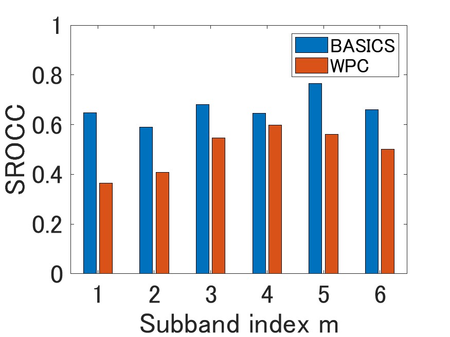
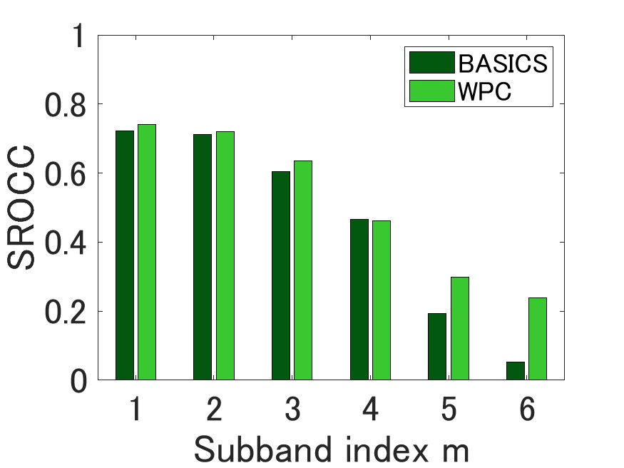
5.2 Experiment 1: Performance of a single score
We evaluated the performance of a single SGW-PCQA score, and (see Fig.4). Since the SROCCs were calculated from only one score in this experiment, SVR was not utilized for integrating multiple scores. As shown in Fig. 4, the SROCC of color-based score was lower for the high-frequency subbands. For the high frequencies of color information, there were many cases where the differences between reference and distorted point clouds were small. We observed that the color signals of a reference point cloud had very few high-frequency components, even for general point clouds other than a simple point cloud shown in Fig.3. Since small high-frequency components are quantized to zero, the compression process does not add high-frequency components. Comparing high-frequency components is not effective in compression noise of color signals, which leads to low SROCCs. Thus, the SROCC of the BASICS dataset consisting only of compression errors was particularly low compared to that of the WPC dataset.
5.3 Experiment 2: Performance of the combination of multiple scores
We investigated the performance achieved by combining multiple scores using SVR. Table 1 shows the PLCC and SROCC of the two datasets. Condition #7 in Table 1, where all geometry scores and three color scores (, , and ) were selected, recorded the best average PLCC and SROCC. Since the SROCCs of color-based scores at high-frequency bands were relatively low as shown in Fig. 4, using the color-based scores at high-frequency bands harmed the correlation with subjective assessment scores.
5.4 Experiment 3: comparison with SOTA methods
We compared the proposed method with conventional FR-PCQA methods [8, 9, 10, 11, 13, 14, 17, 28]. Table 2 presents the results of the comparison experiment with PLCC, SROCC, and average processing time across all the point clouds. SGW-PCQA and SGW-PCQA + in Table 2 adopted condition #7 in Table 1 because it achieved the best results in Section 5.3. The results demonstrate that the proposed SGW-PCQA + achieved the highest PLCC and SROCC. In particular, the PLCC and SROCC of the WPC dataset were improved against our previous study, FRSVR [17]. The PCQA using SGW s were effective with various noise, such as Gaussian noise and down-sampling. For compression noise, the five metrics adopted in FRSVR [17] provided sufficiently high accuracy; however, those metrics can be insufficient for diverse types of noise. In addition, since SGWT s are calculated relatively fast by polynomial approximation [19], SGW-PCQA performed faster computation compared to conventional multiscale metric (e.g., MSGraphSIM [14]).
6 CONCLUSION
This paper introduced an accurate FR-PCQA method using SGW s. The proposed metric demonstrates a great correlation by referring to the SGW s calculated from the coordinate and color signals. In addition, we made the method more accurate by integrating our previous method called FRSVR with the SGW-PCQA metrics by using SVR. In the future, we will consider a more suitable graph construction method for PCQA instead of KNN, which is adopted in the proposed method. Since the previous denoising study [22] has shown that the values of SGW s highly depend on the graph structure, there may be a more suitable graph construction for PCQA.
ACKNOWLEDGEMENTS
This work was supported by the Ministry of Internal Affairs and Communications (MIC) of Japan (Grant no. JPJ000595).
References
- [1] S. Schwarz, M. Preda, V. Baroncini, M. Budagavi, P. Cesar, P. A. Chou, R. A. Cohen, M. Krivokuća, S. Lasserre, Z. Li, J. Llach, K. Mammou, R. Mekuria, O. Nakagami, E. Siahaan, A. Tabatabai, A. M. Tourapis, and V. Zakharchenko, “Emerging MPEG standards for point cloud compression,” IEEE Journal on Emerging and Selected Topics in Circuits and Systems, vol. 9, no. 1, pp. 133–148, 2019.
- [2] Y. Zhou, R. Chen, Y. Zhao, X. Ai, and G. Zhou, “Point cloud denoising using non-local collaborative projections,” Pattern Recognition, vol. 120, pp. 108128, 2021.
- [3] A. Akhtar, Z. Li, G. V. Auwera, L. Li, and J. Chen, “PU-Dense: Sparse tensor-based point cloud geometry upsampling,” IEEE Transactions on Image Processing, vol. 31, pp. 4133–4148, 2022.
- [4] J. He, Z. Fu, W. Hu, and Z. Guo, “Point cloud attribute inpainting in graph spectral domain,” in 2019 IEEE International Conference on Image Processing, 2019, pp. 4385–4389.
- [5] Q. Liu, H. Yuan, H. Su, H. Liu, Y. Wang, H. Yang, and J. Hou, “PQA-Net: Deep no reference point cloud quality assessment via multi-view projection,” IEEE Transactions on Circuits and Systems for Video Technology, vol. 31, no. 12, pp. 4645–4660, 2021.
- [6] Z. Zhang, W. Sun, X. Min, T. Wang, W. Lu, and G. Zhai, “No-reference quality assessment for 3D colored point cloud and mesh models,” IEEE Transactions on Circuits and Systems for Video Technology, vol. 32, no. 11, pp. 7618–7631, 2022.
- [7] A. Chetouani, M. Quach, G. Valenzise, and F. Dufaux, “Deep learning-based quality assessment of 3D point clouds without reference,” in 2021 IEEE International Conference on Multimedia and Expo Workshops, 2021, pp. 1–6.
- [8] R. Mekuria, Z. Li, C. Tulvan, and P. A. Chou, “Evaluation criteria for PCC (point cloud compression),” in ISO/IEC JTC 1/SC29/WG11 Doc., 2016, N16332.
- [9] D. Tian, H. Ochimizu, C. Feng, R. Cohen, and A. Vetro, “Geometric distortion metrics for point cloud compression,” in 2017 IEEE International Conference on Image Processing, 2017, pp. 3460–3464.
- [10] E. Alexiou and T. Ebrahimi, “Towards a point cloud structural similarity metric,” in 2020 IEEE International Conference on Multimedia Expo Workshops, 2020, pp. 1–6.
- [11] G. Meynet, Y. Nehmé, J. Digne, and G. Lavoué, “PCQM: A full-reference quality metric for colored 3D point clouds,” in 2020 Twelfth International Conference on Quality of Multimedia Experience, 2020, pp. 1–6.
- [12] D. Lazzarotto and T. Ebrahimi, “Towards a multiscale point cloud structural similarity metric,” in 25th International Workshop On Multimedia Signal Processing, 2023.
- [13] Q. Yang, Z. Ma, Y. Xu, Z. Li, and J. Sun, “Inferring point cloud quality via graph similarity,” IEEE Transactions on Pattern Analysis and Machine Intelligence, vol. 44, no. 6, pp. 3015–3029, 2022.
- [14] Y. Zhang, Q. Yang, and Y. Xu, “MS-GraphSIM: Inferring point cloud quality via multiscale graph similarity,” in 29th ACM International Conference on Multimedia, 2021, p. 1230–1238.
- [15] M. Tliba, A. Chetouani, G. Valenzise, and F. Dufaux, “Point cloud quality assessment using cross-correlation of deep features,” in Proceedings of the 2nd Workshop on Quality of Experience in Visual Multimedia Applications, 2022, p. 63–68.
- [16] X. Zhou, E. Alexiou, I. Viola, and P. Cesar, “PointPCA+: Extending PointPCA objective quality assessment metric,” in 2023 IEEE International Conference on Image Processing Challenges and Workshops, 2023, pp. 1–5.
- [17] R. Watanabe, S. N. Sridhara, H. Hong, E. Pavez, and A. Ortega, “ICIP 2023 challenge: Full-reference and non-reference point cloud quality assessment methods with support vector regression,” in 2023 IEEE International Conference on Image Processing Challenges and Workshops, 2023, pp. 3654–3658.
- [18] A. Chetouani, G. Valenzise, A. Ak, E. Zerman, M. Quach, M. Tliba, M. A. Kerkouri, and P. L. Callet, “ICIP 2023: Point cloud visual quality assessment grand challenge,” 2023, https://sites.google.com/view/icip2023-pcvqa-grand-challenge/.
- [19] D. K. Hammond, P. Vandergheynst, and R. Gribonval, “Wavelets on graphs via spectral graph theory,” Applied and Computational Harmonic Analysis, vol. 30, no. 2, pp. 129–150, 2011.
- [20] S. Deutsch, A. Ortega, and G. Medioni, “Manifold denoising based on spectral graph wavelets,” in 2016 IEEE International Conference on Acoustics, Speech and Signal Processing, 2016, pp. 4673–4677.
- [21] M. A. Irfan and E. Magli, “Joint geometry and color point cloud denoising based on graph wavelets,” IEEE Access, vol. 9, pp. 21149–21166, 2021.
- [22] R. Watanabe, K. Nonaka, E. Pavez, T. Kobayashi, and A. Ortega, “Graph wavelet-based point cloud geometric denoising with surface-consistent non-negative kernel regression,” in 2023 IEEE International Conference on Acoustics, Speech and Signal Processing, 2023, pp. 1–5.
- [23] E. Alexiou and T. Ebrahimi, “Exploiting user interactivity in quality assessment of point cloud imaging,” in 2019 Eleventh International Conference on Quality of Multimedia Experience, 2019, pp. 1–6.
- [24] H. R. Sheikh and A. C. Bovik, “Image information and visual quality,” IEEE Transactions on Image Processing, vol. 15, no. 2, pp. 430–444, 2006.
- [25] Z. Wang, A. C. Bovik, H. R. Sheikh, and E. P. Simoncelli, “Image quality assessment: from error visibility to structural similarity,” IEEE Transactions on Image Processing, vol. 13, no. 4, pp. 600–612, 2004.
- [26] Z. Wang and Q. Li, “Information content weighting for perceptual image quality assessment,” IEEE Transactions on Image Processing, vol. 20, no. 5, pp. 1185–1198, 2011.
- [27] Q. Liu, H. Su, Z. Duanmu, W. Liu, and Z. Wang, “Perceptual quality assessment of colored 3D point clouds,” IEEE Transactions on Visualization and Computer Graphics, vol. 29, no. 8, pp. 3642–3655, 2023.
- [28] E. Alexiou and T. Ebrahimi, “Point cloud quality assessment metric based on angular similarity,” in 2018 IEEE International Conference on Multimedia and Expo, 2018, pp. 1–6.
- [29] I. Lissner and P. Urban, “Toward a unified color space for perception-based image processing,” IEEE Transactions on Image Processing, vol. 21, no. 3, pp. 1153–1168, 2012.
- [30] D. I. Shuman, S. K. Narang, P. Frossard, A. Ortega, and P. Vandergheynst, “The emerging field of signal processing on graphs: Extending high-dimensional data analysis to networks and other irregular domains,” IEEE Signal Processing Magazine, vol. 30, no. 3, pp. 83–98, 2013.
- [31] N. Leonardi and D. Van De Ville, “Tight wavelet frames on multislice graphs,” IEEE Transactions on Signal Processing, vol. 61, no. 13, pp. 3357–3367, 2013.
- [32] J. Platt, “Sequential minimal optimization: A fast algorithm for training support vector machines,” Tech. Rep. MSR-TR-98-14, Microsoft, 1998.
- [33] A. Ak, E. Zerman, M. Quach, A. Chetouani, A. Smolic, G. Valenzise, and P. L. Callet, “Basics: Broad quality assessment of static point clouds in a compression scenario,” IEEE Transactions on Multimedia, pp. 1–13, 2024.
- [34] H. Su, Z. Duanmu, W. Liu, Q. Liu, and Z. Wang, “Perceptual quality assessment of 3D point clouds,” in 2019 IEEE International Conference on Image Processing, 2019, pp. 3182–3186.