Small-scale and large-scale dynamos in global convection simulations of solar-like stars

Abstract

Context. It has been recently shown numerically that a small-scale dynamo (SSD) instability could be possible in solar-like low magnetic Prandtl number ($\mbox{\rm Pr}_{\rm M}$) plasmas. It has been proposed that the presence of SSD can potentially have a significant impact on the dynamics of the large-scale dynamo (LSD) in the stellar convection zones. Studying these two dynamos, SSD and LSD, together in a global magnetoconvection model requires high-resolution simulations and large amounts of computational resources.

Aims. Starting from a well-studied global convective dynamo model that produces cyclic magnetic fields, we systematically increased the resolution and lowered the diffusivities to enter the regime of Reynolds numbers that allow for the excitation of SSD on top of the LSD. We studied how the properties of convection, generated differential rotation profiles, and LSD solutions change with the presence of SSD.

Methods. We performed semi-global convective dynamo simulations in a spherical wedge with the Pencil Code. The resolutions of the models were increased in 4 steps by a total factor of 16 to achieve maximal fluid and magnetic Reynolds numbers of over 500.

Results. We found that the differential rotation is strongly quenched by the presence of the LSD and SSD. Even though the small-scale magnetic field only mildly decreases increasing Re, the large-scale field strength decreases significantly. We do not find the SSD dynamo significantly quenching the convective flows as claimed recently by other authors; in contrast, the convective flows first grow and then saturate for increasing Re. Furthermore, the angular momentum transport is highly affected by the presence of small-scale magnetic fields, which are mostly generated by LSD. These fields not only change the Reynolds stresses, but also generate dynamically important Maxwell stresses. The LSD evolution in terms of its pattern and field distribution is rather independent of the increase in Re and $\mbox{\rm Re}_{\rm M}$.

Conclusions. At high fluid and magnetic Reynolds numbers, an SSD, in addition to the LSD, can be excited, and both have a strong influence on angular momentum transport. Hence, it is important to study both dynamos and their interplay together to fully understand the dynamics of the Sun and other stars.

1 Introduction

The Sun and other cool stars exhibit large-scale magnetic fields, which in some cases show cyclic variations (e.g. Baliunas et al. 1995; Boro Saikia et al. 2018; Olspert et al. 2018). This is associated with a large-scale dynamo (LSD) operating in the stellar convection zones producing complex magnetic surface features (Charbonneau 2014). Besides the LSD, a small-scale dynamo (SSD) has been proposed to be present in these stars (e.g. Rempel et al. 2023). In contrast to an LSD, the SSD does not need any large-scale rotation, shear or stratification to operate and the scales of its magnetic field are at or below the characteristic scales of the flow (Brandenburg & Subramanian 2005). There is some debate whether or not an SSD can operate in solar-like stars. These doubts were supported on one hand by numerical simulations, which show that an SSD is increasingly harder to excite when approaching the solar parameters (Schekochihin et al. 2005), and on the other hand by the inconclusive results of small-scale field observations on the Sun (Bellot Rubio & Orozco Suárez 2019). Some observal studies show a cyclic modulation of the inter-network field, hence a connection to the cylic large-scale magnetic field, whereas some studies show that the these fields are rather cyclic independent. The doubts based on numerical simulations, however, were recently alleviated by high-resolution simulations at magnetic Prandtl numbers approaching the solar value closer than ever before (Warnecke et al. 2023). These simulations show that an SSD is not only possible at these very low magnetic Prandtl numbers, but becomes even easier to excite in this limit. These results hint towards a possible dynamical importance of the SSD in the Sun and solar-like stars.

The influence of SSD on the dynamics and LSD has been studied with simplified setups (Vainshtein & Cattaneo 1992; Tobias & Cattaneo 2013; Squire & Bhattacharjee 2015; Singh et al. 2017; Väisälä et al. 2021), while only recently global convective dynamo simulations (Käpylä et al. 2023) were able to reach the regime where both LSD and SSD are excited and can therefore be studied together (Hotta et al. 2016; Käpylä et al. 2017a; Hotta & Kusano 2021; Hotta et al. 2022, hereafter HK21, HKS22). In Hotta et al. (2016), the authors found that the SSD suppresses small-scale flows mimicing properties of an enhanced magnetic diffusivity, this in-turn enhances the LSD. Käpylä et al. (2017a), on the other hand found that the SSD quenches differential rotation, which being one of the main dynamo drivers consequently supressed the LSD in some of their cases. The influence of the magnetic field on the differential rotation has been investigated in many previous studies (e.g. Fan & Fang 2014; Karak et al. 2015; Käpylä et al. 2016; Warnecke et al. 2013, 2016; Brun et al. 2022; Käpylä et al. 2023), yet the most relevant for the present work is Käpylä et al. (2017a), because of the presence of an SSD. In this study the authors found that an increase in $\mbox{\rm Re}_{\rm M}$ leads to strong suppression of the differential rotation. The authors suggested further that the Maxwell stresses becomes comparable to the Reynolds stresses and therefore only a weak differential rotation can be generated. They found that the increase in Maxwell stresses is partly due to a strong SSD being present. HK21 and HKS22 found that the efficient SSD in their simulation is able to reshape an anti-solar differential rotation into a solar one for increasing Reynolds numbers. Taken that the results obtained with different approaches diverge quite significantly, it is necessary to further investigate the role of SSD in LSD-active and differentially rotating systems. As magnetic fluctuations originate from through different sources, namely SSD-action itself and tangling of the mean field through convective turbulence, it is also important to gain further insights into the role of these two contributions separately. These are among the most important goals of this paper.

Since the pioneering work of Brandenburg (2016) and Käpylä et al. (2017b), it has been known that a more realistic description of the radiative heat diffusivity using a Kramers’ opacity based term can lead to the formation of sub-adiabatic layers at the base of the convection zone (e.g. Käpylä et al. 2019; Viviani & Käpylä 2021). How the shape and depth of these layers depend on the Reynolds number or the presence of SSD and LSD has only been studied in a few Cartesian simulations (Hotta 2017; Käpylä 2019c, 2021) but not in a global setup.

In this paper we present a study of a global convective dynamo model in an azimuthal wedge of a spherical shell using a Kramers’ opacity based heat conductivity. We increased the resolution systematically from 128x256x128 to 2048x4096x2048 grid points to reach fluid and magnetic Reynolds numbers ($\mbox{\rm Re}_{\rm M}$) of above 500. This parameter regime allows us to investigate the LSD and SSD interaction in detail. To separately study the effect of the LSD and SSD on the overall dynamics, for each configuration, we run: a full model, where potentially both LSD and SSD can be excited; a ”reduced” model where the large-scale field is taken out to excite only an SSD; a hydrodynamic model in which no magnetic field is present. The paper is organized as follows: in Sect. 2 we present our model and setup, in Sect. 3 we discuss in detail the results, and in Sect. 4 we present our conclusions. Additional informations are given in the Appendix A to C.

Table 1: Summary of runs.

Run Resolution Ta[$10^{8}$] $\overline{}\mbox{\rm Ra}_{\rm Kram}$[$10^{7}$] $\overline{}\mbox{\rm Ra}_{\rm SGS}$[$10^{7}$] $\widetilde{\mbox{\rm Ra}}_{\rm SGS}$ Pr Re Co SLD $\Delta{\theta}_{\nu}$ $\Delta{\theta}_{\eta}$ $\Delta_{\nu\eta}$ 0M $\phantom{1}128\times\phantom{1}256\times\phantom{1}128$ 1.25 73 1.2 48 5.13 27 10.4 0H $\phantom{1}128\times\phantom{1}256\times\phantom{1}128$ 1.25 73 1.2 48 5.13 28 9.9 yes 1M $\phantom{1}256\times\phantom{1}512\times\phantom{1}256$ 5.00 280 5.9 94 1.52 61 9.3 $5^{\circ}$ $5^{\circ}$ 2 1H $\phantom{1}256\times\phantom{1}512\times\phantom{1}256$ 5.00 280 5.9 94 1.52 66 8.5 yes 2M $\phantom{1}512\times 1024\times\phantom{1}512$ 20.0 1050 23.7 149 0.58 127 8.9 $5^{\circ}$ $5^{\circ}$ 5 2S $\phantom{1}512\times 1024\times\phantom{1}512$ 20.0 1050 23.7 149 0.58 139 8.1 $5^{\circ}$ $5^{\circ}$ 5 2H $\phantom{1}512\times 1024\times\phantom{1}512$ 20.0 1050 23.7 149 0.58 143 7.9 yes $5^{\circ}$ 5 3M $1024\times 2048\times 1024$ 80.0 3155 71.5 178 0.27 255 8.9 $17^{\circ}$ $17^{\circ}$ 5 3S $1024\times 2048\times 1024$ 80.0 3155 71.5 178 0.27 265 8.5 $17^{\circ}$ $5^{\circ}$ 5 3H $1024\times 2048\times 1024$ 80.0 3155 71.5 178 0.27 287 7.9 yes $17^{\circ}$ 5 4M $2048\times 4096\times 2048$ 320.0 7536 185.9 184 0.12 517 8.7 $17^{\circ}$ $5^{\circ}$ 5 4M2 $2048\times 4096\times 2048$ 320.0 7536 185.9 184 0.12 549 8.5 $17^{\circ}$ $5^{\circ}$ 5 4S $2048\times 4096\times 2048$ 320.0 7536 185.9 184 0.12 550 8.2 $17^{\circ}$ $5^{\circ}$ 5

2 Model and setup

The stellar convection zone is modelled in spherical geometry ($r,\theta,\phi$) as a shell with a depth $D$ similar to that in the Sun ($0.7R\leq r\leq R$) where $R$ is the radius of the star. We leave out the poles ($\theta_{0}\leq\theta\leq\pi-\theta_{0}$ with $\theta_{0}=15^{\circ}$) and restrict our model to a quarter of the sphere (a “wedge”, with $0\leq\phi\leq\pi/2$), both for numerical reasons. Our model is similar to the ones of Käpylä et al. (2013), Käpylä et al. (2016), and Käpylä et al. (2019) and we refer to these papers for a detailed description.

We solve the fully compressible MHD equations in terms of the vector potential $A$ (ensuring the solenoidality of $B$), the velocity $u$, the specific entropy $s$, and the density $\rho$, and employ an ideal-gas equation of state. We include the rotational effects by adding the Coriolis force $2\mbox{\boldmath$u$}{}\times\bm{\Omega}_{0}$ to the momentum equation where $\bm{\Omega}_{0}=\Omega_{0}(\cos\theta,-\sin\theta,0)$ and $\Omega_{0}$ is the angular velocity of the modeled star’s co-rotating frame, in which the plasma has zero total angular momentum. We choose constant magnetic diffusivity $\eta$ and kinematic viscosity $\nu$, except near the latitudinal boundaries, where we add in some of the runs for numerical reasons $\nu$ and $\eta$ profiles, increasing with $\theta$ towards the boundaries across an interval $\Delta\theta$, see Appendix A for details. In our model, the diffusive heat flux has two contributions. The first one models the radiative heat flux as $\mbox{\boldmath$F$}{}^{\rm rad}=-K\mbox{\boldmath$\nabla$}{}T$ with temperature and density dependent radiative heat conductivity $K$, based on Kramers’ opacity, so that $K$ is given by

$$K(\rho,T)=K_{0}\left({\rho\over\rho_{0}}\right)^{-2}\left({T\over T_{0}}\right)^{13/2}.$$ (1)

and the reference values $\rho_{0}$ and $T_{0}$ are set to the corresponding values at the bottom of the domain in the initial (hydrostatic) state; for details see Barekat & Brandenburg (2014), Käpylä et al. (2019) and Viviani & Käpylä (2021). The second contribution mimics the heat flux of the unresolved or sub-grid-scale (SGS) convection and stabilises the system. This SGS heat flux is given by $\mbox{\boldmath$F$}{}^{\rm SGS}=-\chi_{\rm SGS}\rho T\mbox{\boldmath$\nabla$}{}s$. As in Käpylä et al. (2013), $\chi_{\rm SGS}$ follows a smooth radial profile, which is zero at the bottom of the domain, constant ($\chi_{\rm SGS}=\chi_{\rm m}^{\rm SGS}$) in the bulk and maximal near the top transporting there the majority of the heat. For some of the hydrodynamic runs, we needed to add a slope-limited diffusion, acting on density and velocity, to stabilise the system, see Appendix B for details.

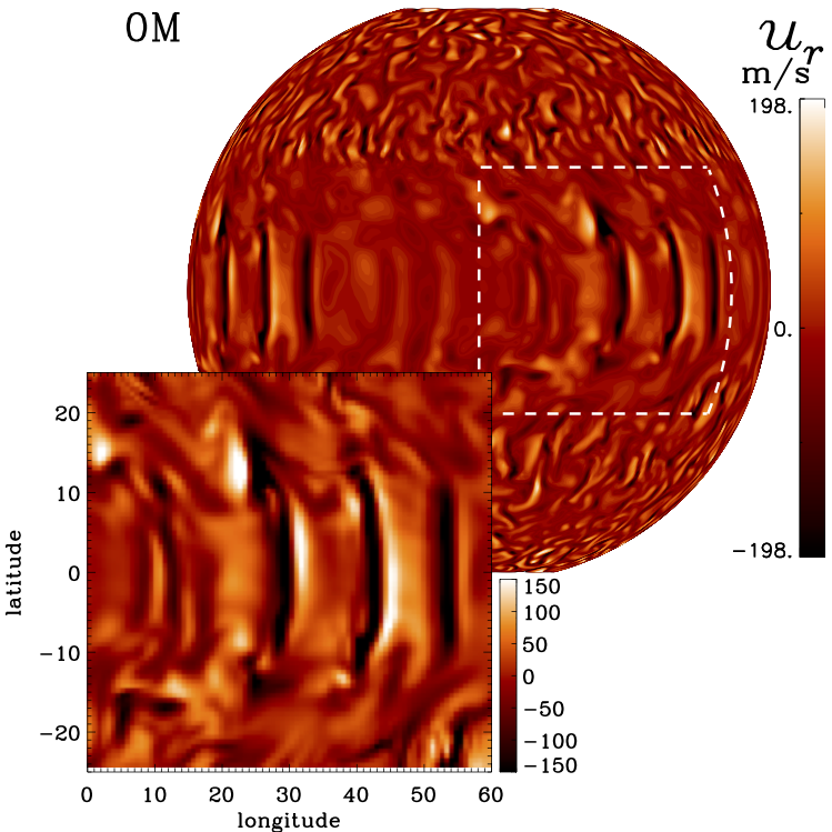
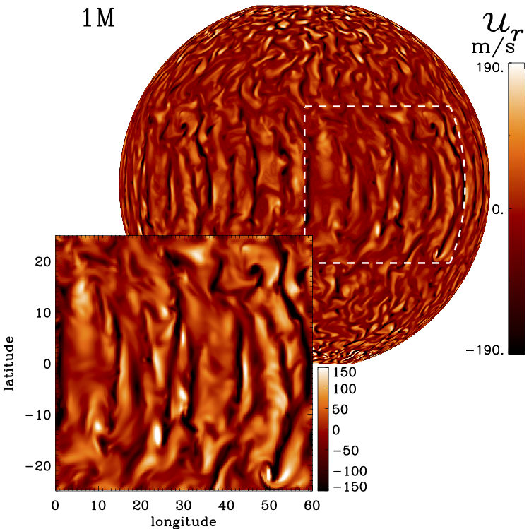
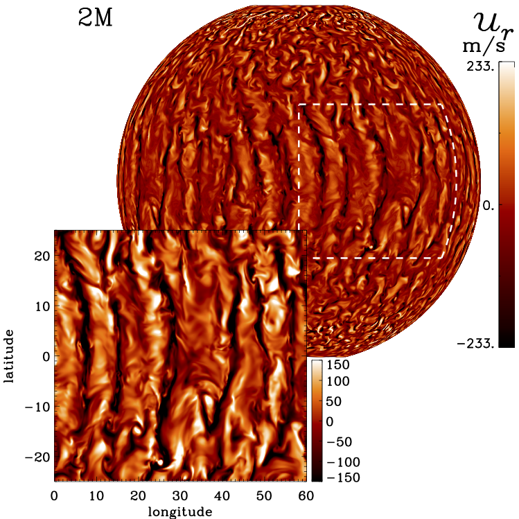
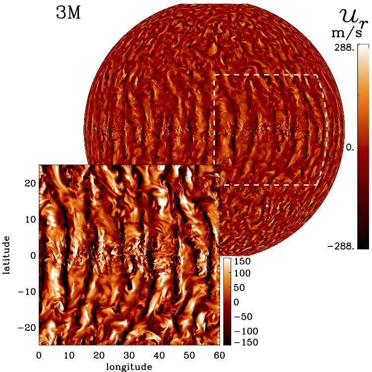
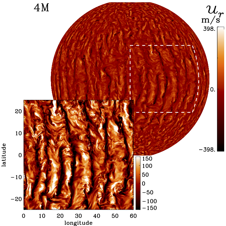
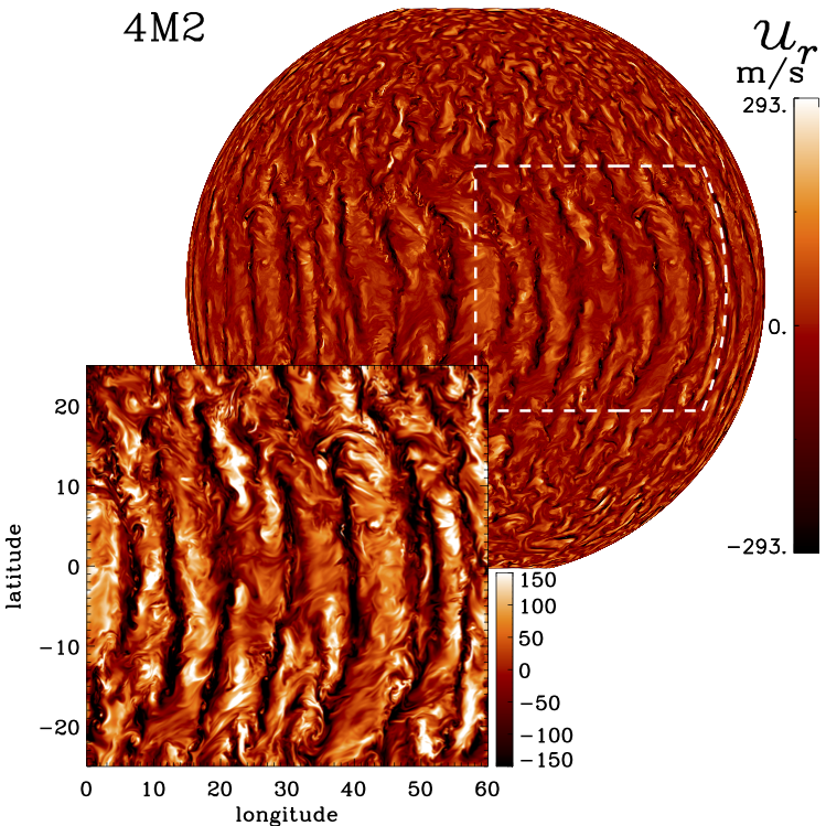
Figure 1: Radial velocity $u_{r}$ at $r=0.98\,R$ with a low-latitude cut-out, for all M runs in the saturated stage. The wedge is duplicated to form a half sphere.

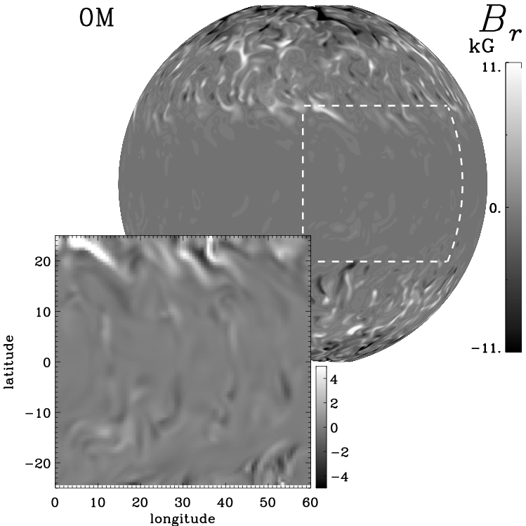
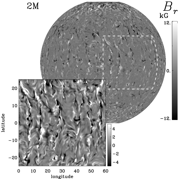
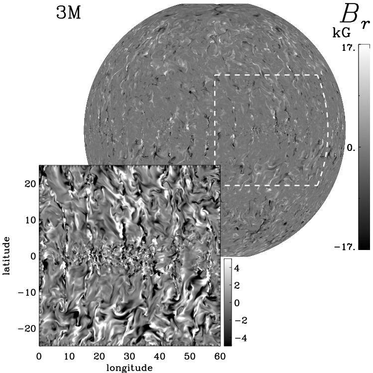
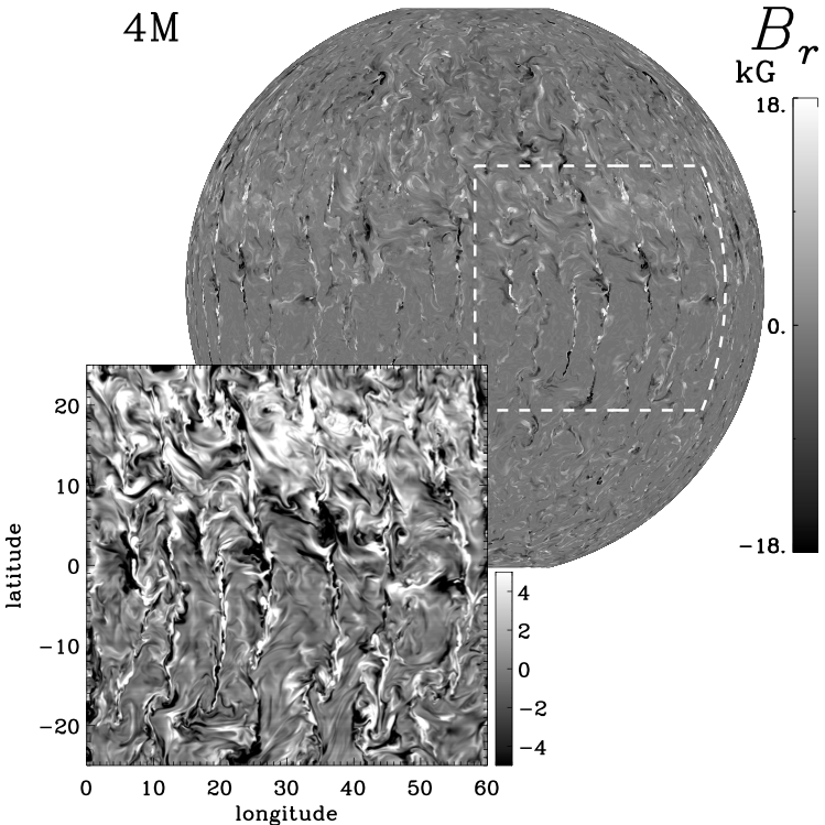
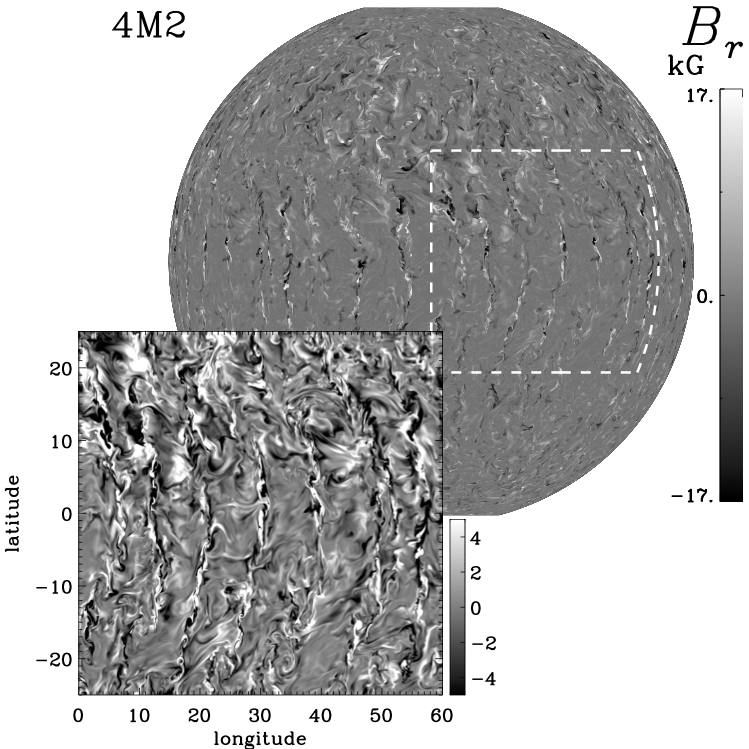
Figure 2: Radial magnetic field $B_{r}$ at $r=0.98\,R$ for all M runs. Otherwise as Fig. 1.

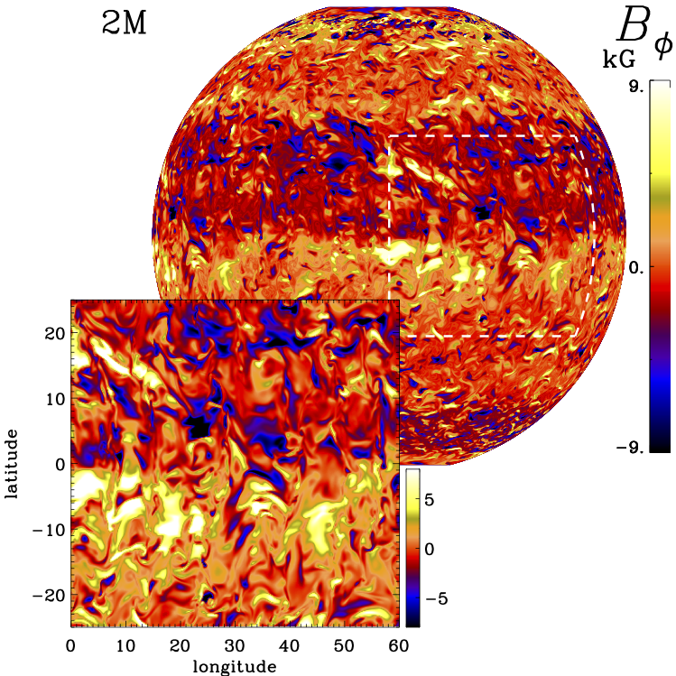
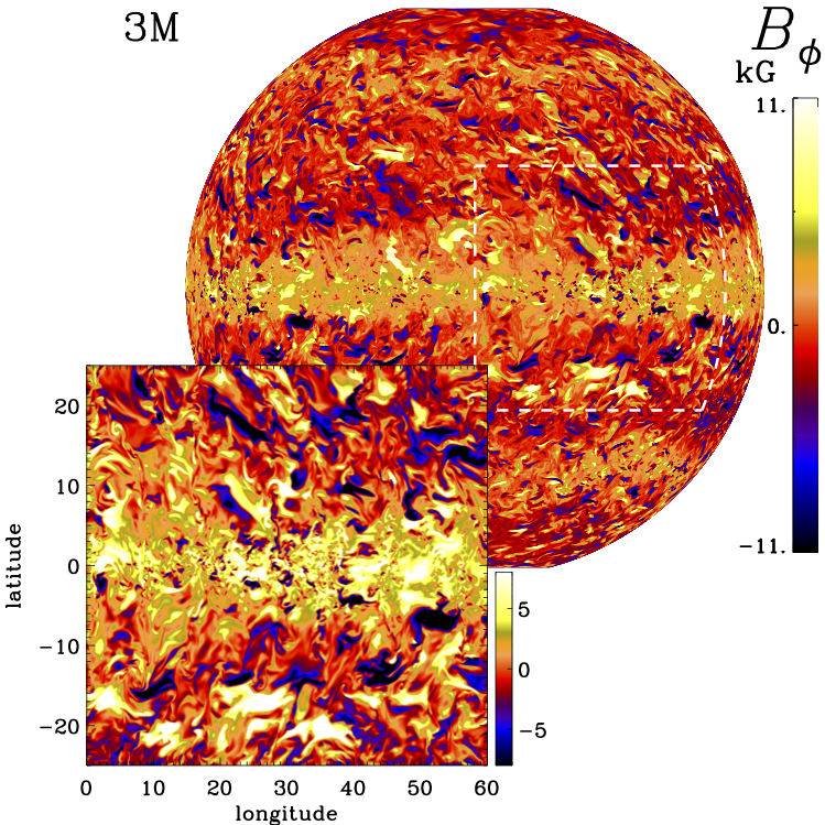
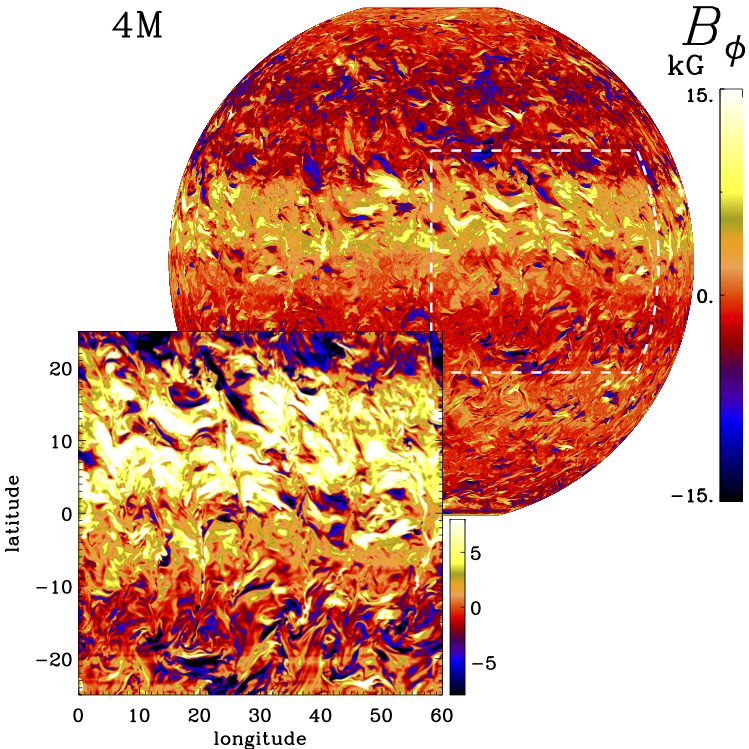
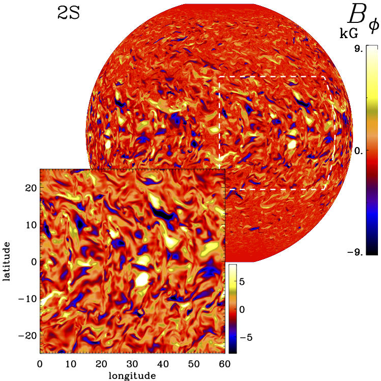
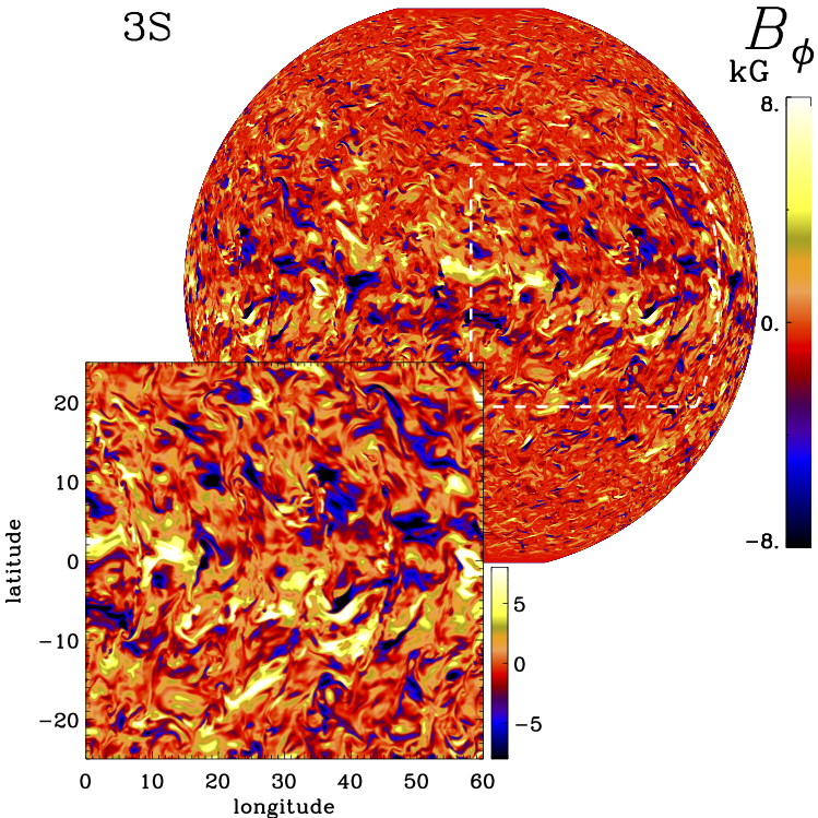
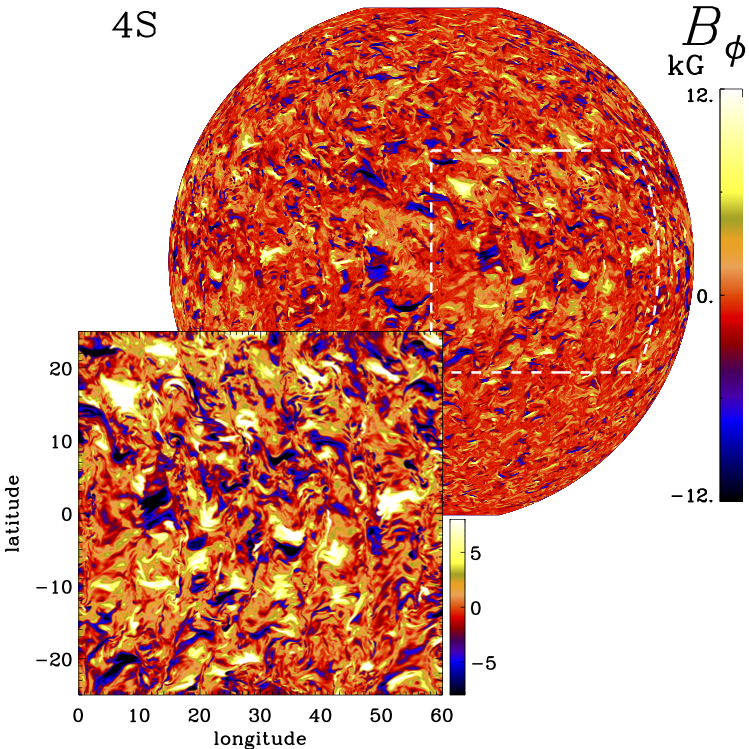
Figure 3: Azimuthal magnetic field $B_{\phi}$ at $r=0.98\,R$ for all M runs with an SSD and the corresponding S runs. Otherwise as Fig. 1.

The plasma is heated at the bottom by a constant heat flux and cooled at the top by black-body radiation. The velocity $u$ is stress-free on all radial and latitudinal boundaries, and the entropy $s$ has zero derivatives at the latitudinal boundaries. At the lower radial and at the latitudinal boundaries, we choose the magnetic field $B$ to follow a perfect conductor while being purely radial at the top. In the $\phi$ direction, the boundary conditions for all the quantities are periodic.

Our runs are defined by the following non-dimensional input parameters: We define a normalized angular frequency and the Taylor number

$$\tilde{\Omega}=\Omega_{0}/\Omega_{\odot},\quad\mbox{\rm Ta}=\left[2\Omega_{0}(0.3R)^{2}/\nu\right]^{2},$$ (2)

where $\Omega_{\odot}=2.7\times 10^{-6}\,{\rm s}^{-1}$ is the rotation rate of the Sun, while the thermal, SGS-thermal, and magnetic Prandtl numbers are

$$\mbox{\rm Pr}={\nu\over\chi_{\rm m}},\quad\mbox{\rm Pr}_{\rm SGS}={\nu\over\chi_{\rm m}^{\rm SGS}},\quad\mbox{\rm Pr}_{\rm M}={\nu\over\eta},$$ (3)

where $\chi_{\rm m}=K(r=r_{\rm m})/\rho c_{\rm P}$ is the thermal diffusivity based on Kramers’ opacity in the middle of the convection zone ($r=r_{\rm m}$), see Equation (1), and $c_{\rm P}$ is the specific heat capacity at constant pressure. As $K$ depends on local density and temperature, we use a one-dimensional hydrostatic model to determine $K$ and $\rho$ for Pr. We note that Pr in the saturated stage can be significantly different from the hydrostatic model. Additionally, we define two Rayleigh numbers calculated from the same hydrostatic model. One is based on the Kramers heat diffusivity $\chi$

$$\mbox{\rm Ra}_{\rm Kram}(r)\!=\!\frac{GM(0.3R)^{4}}{\nu\chi(r)R^{2}}\bigg{(}-\frac{1}{c_{\rm P}}\frac{{\rm d}s_{\rm hs}}{{\rm d}r}\bigg{)},$$ (4)

the other on the SGS heat diffusivity $\chi_{\rm SGS}$

$$\mbox{\rm Ra}_{\rm SGS}(r)\!=\!\frac{GM(0.3R)^{4}}{\nu\chi_{\rm SGS}(r)R^{2}}\bigg{(}-\frac{1}{c_{\rm P}}\frac{{\rm d}s_{\rm hs}}{{\rm d}r}\bigg{)},$$ (5)

where $s_{\rm hs}$ is the specific entropy in the hydrostatic model, $G$ is the gravitational constant, and $M$ is the total mass of the star. As the Rayleigh numbers strongly depend on $r$ and are not always positive in the middle of the domain (as in the non-Kramers runs), we average them over their logarithmised positive contribution $\ln\mbox{\rm Ra}_{+}$:

$$\overline{}\mbox{\rm Ra}=\exp\,\langle\ln\mbox{\rm Ra}_{+}(r)\rangle_{r},$$ (6)

where the subscript $r$ marks radial averaging.

To estimate the supercriticality, we define a further Rayleigh number, in which the reduction of supercriticality due to rotation is compensated by the Taylor number $\widetilde{\mbox{\rm Ra}}=\overline{}\mbox{\rm Ra}/\mbox{\rm Ta}^{2/3}$, following (e.g. Chandrasekhar 1961; Roberts 1968; Barik et al. 2023).

We further characterise our simulations by the fluid and magnetic Reynolds numbers together with the Coriolis number

$$\mbox{\rm Re}=\frac{u_{\rm rms}}{\nu k_{\rm f}},\quad\mbox{\rm Re}_{\rm M}=\frac{u_{\rm rms}}{\eta k_{\rm f}},\quad\mbox{\rm Co}={2\Omega_{0}\over u_{\rm rms}k_{\rm f}},$$ (7)

where $k_{\rm f}=2\pi/0.3R\approx 21/R$ is an estimate of the wavenumber of the largest eddies in the domain and $u_{\rm rms}=\sqrt{(3/2)\langle u_{r}^{2}+u_{\theta}^{2}\rangle_{r\theta\phi t}}$ is the rms velocity; the subscripts indicate averaging over $r$, $\theta$, $\phi$ and a time interval covering the saturated state. These non-dimensional input and solution parameters are given in Table LABEL:runs for all runs. To summarize, we use the same model as in Käpylä et al. (2016) except that we apply here Kramers heat conductivity instead of a fixed conductivity profile.

For our analysis throughout the paper, we decompose each field into a mean (axisymmetric) and a fluctuating part, which are indicated by an overbar and a prime, respectively, for example, $\mbox{\boldmath$B$}{}=\overline{\mbox{\boldmath$B$}}{}+\mbox{\boldmath$B$}{}^{\prime}$ and $\mbox{\boldmath$u$}{}=\overline{\mbox{\boldmath$u$}}{}+\mbox{\boldmath$u$}{}^{\prime}$. Restricting to fluctuating fields, we define an $r$- and $\theta$-dependent turbulent rms velocity as $u^{\prime}_{\rm rms}(r,\theta)={\left\langle\,\overline{{\bm{u}}^{\prime\,2}}\,\right\rangle_{t}}{}^{\!\!1/2}$, turbulent rms magnetic field strength $B^{\prime}_{\rm rms}(r,\theta)={\left\langle\,\overline{{\bm{B}}^{\prime\,2}}\,\right\rangle_{t}}{}^{\!\!1/2}$ and turbulent equipartition field strength $B_{\rm eq}(r,\theta)=u^{\prime}_{\rm rms}(\mu_{0}\overline{\rho})^{1/2}$, where $\mu_{0}$ is the magnetic vacuum permeability.

The total kinetic energy density is defined as

$$E_{\rm kin}^{\rm tot}={\textstyle{1\over 2}}\left\langle\rho\mbox{\boldmath$u$}{}^{2}\right\rangle_{V},$$ (8)

which is further decomposed into the energy densities of the fluctuating velocity, the differential rotation, and the meridional circulation:

$$E_{\rm kin}^{\rm flu}={\textstyle{1\over 2}}\left\langle\rho\mbox{\boldmath$u$}{}^{\prime\,2}\right\rangle_{V}\!,\>E_{\rm kin}^{\rm dif}={\textstyle{1\over 2}}\left\langle\rho\overline{u}_{\phi}^{2}\right\rangle_{V}\!,\>E_{\rm kin}^{\rm mer}={\textstyle{1\over 2}}\left\langle\rho\left(\overline{u}_{r}^{2}+\overline{u}_{\theta}^{2}\right)\right\rangle_{V}.$$ (9)

Here, $\left\langle\right\rangle_{V}$ indicates volume averaging. In a similar way, the total magnetic energy density is defined as

$$E_{\rm mag}^{\rm tot}={\textstyle\frac{1}{2\mu_{0}}}\left\langle\mbox{\boldmath$B$}{}^{2}\right\rangle_{V},$$ (10)

and can be decomposed into the energy densities of the fluctuating fields, along with those of the toroidal and poloidal mean magnetic fields:

$$E_{\rm mag}^{\rm flu}={\textstyle\frac{1}{2\mu_{0}}}\left\langle\mbox{\boldmath$B$}{}^{\prime\,2}\right\rangle_{V}\!,\>E_{\rm mag}^{\rm tor}={\textstyle\frac{1}{2\mu_{0}}}\left\langle\overline{B}_{\phi}^{2}\right\rangle_{\!V}\!,\>E_{\rm mag}^{\rm pol}={\textstyle\frac{1}{2\mu_{0}}}\left\langle\overline{B}_{r}^{2}+\overline{B}_{\theta}^{2}\right\rangle_{V}.$$ (11)

The analysis and quantities presented in our paper are performed and calculated from the saturated stage of the simulations. The rescaling of our simulations to physical units is based on the solar rotation rate $\Omega_{\odot}=2.7\times 10^{-6}\,{\rm s}^{-1}$, solar radius $R=7\times 10^{8}\,{\rm m}$, density at the bottom of the domain $\rho(0.7R)=200\,{\rm kg}/\,{\rm m}^{3}$, and $\mu_{0}=4\pi\cdot 10^{-7}$ H m^-1. All simulations were performed using the Pencil Code (Pencil Code Collaboration et al. 2021).

3 Results

Our goal is to study the LSD and SSD together in a setup including a physically motivated heat conductivity based on Kramers’ opacity. As our starting point, we use the model of Käpylä et al. (2016), with the only difference that the prescribed heat conductivity is replaced by a Kramers-opacity based one; this represents Run 0M. We then lower, step by step, the viscosity $\nu$, the magnetic diffusivity $\eta$ and the SGS heat diffusivity $\chi_{\rm SGS}$ making the simulation gradually more turbulent while keeping $\mbox{\rm Pr}_{\rm SGS}$ and $\mbox{\rm Pr}_{\rm M}$ constant. At each step, indicated by the number in the run label, the diffusivities are halved, leading to a total reduction by factor of 16 from Set 0 to Set 4. Technically, this requires doubling the resolution and remeshing the run at each step, and eventually running the simulation in the saturation regime for a sufficient time span.

To study the effects of the SSD in isolation and to check whether it is indeed present, we fork each MHD run in two, having identical setups: In the first one, denoted with ‘S”, we remove the mean field $\overline{\mbox{\boldmath$B$}}{}$ at every fifth time step, hence no LSD can develop. When an SSD is sustained, we study it in detail. In the second one, denoted by “M”, mean-field removal is not applied, hence the LSD can develop freely. Finally, we also perform the corresponding hydrodynamic simulations, denoted by “H”. Note that Run 4M2 is basically the same as 4M except that we have not re-meshed and re-started from 3M, which has an LSD, but re-started from 4S, where only an SSD is present, yet allowing for the growth of the LSD after the re-start. Our motivation was here to study whether an LSD can be excited and grow in the presence of already existing strong magnetic fluctuations. Runs 0M to 2M are similar to Runs G1 to G3 in Käpylä et al. (2017a), where the difference is in the use of the Kramers-based heat conductivity in our work and in a normal magnetic field condition at the latitudinal boundaries in G2 & G3.

All runs are listed in Table LABEL:runs with their control and solution parameters. We note that an SSD is present in Sets 2–4, implying that its critical magnetic Reynolds number lies between roughly 60 and 130. This is consistent with the study of Käpylä et al. (2017a), where an SSD is typically found for $\mbox{\rm Re}_{\rm M}>60$. Interestingly, run G2 of Käpylä et al. (2017a) has an SSD with $\mbox{\rm Re}_{\rm M}=66$ in contrast to our Run 2M with $\mbox{\rm Re}_{\rm M}=61$ that does not excite an SSD. Either the SSD is very close to critical or the slight differences in the setups are causal. We note here that $\mbox{\rm Re}_{\rm M}$ in both their and our work is only an average and hence does not reflect the detailed local dynamics. The critical $\mbox{\rm Re}_{\rm M}$ found in our work is somewhat higher than what is obtained from theoretical models for smooth velocity fields with low compressibility, yielding predictions of the order of 30–60 (Brandenburg & Subramanian 2005), and $\mbox{\rm Re}_{\rm M}=30-50$ from simple isothermal forced turbulence models (e.g. Schekochihin et al. 2005; Väisälä et al. 2021; Warnecke et al. 2023).

Decreasing the diffusivities leads to a strong increase in the Rayleigh numbers $\overline{}\mbox{\rm Ra}_{\rm Kram}$ and $\overline{}\mbox{\rm Ra}_{\rm SGS}$ by a factor of more than 100. However, as also the Taylor number, Ta, increases significantly by a factor of nearly 300, we need to look at the compensated Rayleigh number $\widetilde{\mbox{\rm Ra}}_{\rm SGS}$ to assess whether or not the supercriticality increases. Indeed, $\widetilde{\mbox{\rm Ra}}_{\rm SGS}$ is nearly 4 times larger in the run with the lowest diffusivities than in the one with the highest. The rotational influence on the convection in terms of Co decreases only slightly when the diffusivities are decreased because the turbulent convection becomes slightly stronger. Pr is above unity for Sets 0 and 1 and below unity for Sets 2–4, indicating that heat conduction (in the middle of the convection zone) is dominated by the SGS contribution for Sets 0 and 1 and by the Kramers contribution otherwise, however, one needs to take into account that these two terms involve different gradients.

3.1 Overview of the dynamics

As shown in Fig. 1 for all the M runs, the radial velocity becomes more turbulent and develops progressively more small-scale structures when lowering the diffusivities, hence increasing the Reynolds numbers. For all runs, prominent thermal Rossby waves, also known as Busse columns or banana cells (e.g. Busse 1970, 1976; Featherstone & Hindman 2016; Bekki et al. 2022) are present outside the tangent cylinder in the equatorial regions, in agreement with earlier models and theoretical expectations. Interestingly, the longitudinal degree of these waves does not vary much with increasing Reynolds number, being mostly between $m=32$ and $m=40$ for all runs; see Appendix C for a more detailed analysis.

In Fig. 2, we show the corresponding radial magnetic field close to the surface for all the M runs. Near the equator, the radial magnetic field is mostly concentrated in the downflow lanes of the banana cells where it forms complex structures with small bipolar patches. The radial field is mostly dominated by magnetic fluctuations, while the mean field is not visible near the equator. At higher latitudes in Runs 0M–2M, one can see hints of longitudinal bands of same polarity tracing the weak mean radial field. For 3M, 4M and 4M2, these patterns are no so clearly visible anymore.

In Fig. 3, we show the azimuthal magnetic field for Runs 2M, 2S, 3M, 3S, 4M, and 4S. For this component, the difference between Sets S and M is most pronounced. In the M runs, the mean field is clearly visible at all covered latitudes. The magnetic fluctuations in these runs are also present ubiquitously. In Run 2S, the fluctuating magnetic field is more concentrated near the equator. The fluctuations become distributed over progressively wider latitude ranges when the Reynolds numbers are increased, see Runs 3M to 4M. Interestingly, the banana cell pattern does not produce a strong imprint on the azimuthal magnetic field structure.

Table 2: Energy densities for all runs.

Run $E^{\rm tot}_{\rm kin}$ $E^{\rm dif}_{\rm kin}$ $E^{\rm mer}_{\rm kin}$ $E^{\rm flu}_{\rm kin}$ $E^{\rm tot}_{\rm mag}$ $E^{\rm tor}_{\rm mag}$ $E^{\rm pol}_{\rm mag}$ $E^{\rm flu}_{\rm mag}$ $E^{\rm tot}_{\rm mag}/E^{\rm tot}_{\rm kin}$ $E^{\rm flu}_{\rm mag}/E^{\rm flu}_{\rm kin}$ 0M 2.225 1.562 0.006 0.658 0.369 0.072 0.048 0.250 0.166 0.379 0H 17.089 16.159 0.010 0.920 1M 1.267 0.546 0.006 0.716 0.604 0.172 0.047 0.385 0.476 0.538 1H 4.397 3.457 0.010 0.930 2M 0.933 0.213 0.005 0.715 0.763 0.198 0.044 0.521 0.819 0.729 2S 5.643 4.503 0.010 1.130 0.140 0.000 0.000 0.140 0.025 0.124 2H 8.697 7.514 0.012 1.171 3M 0.923 0.197 0.005 0.721 0.510 0.057 0.023 0.430 0.553 0.597 3S 1.448 0.542 0.007 0.900 0.228 0.000 0.000 0.228 0.158 0.254 3H 7.352 6.347 0.011 0.993 4M 0.854 0.144 0.005 0.705 0.876 0.190 0.030 0.656 1.026 0.931 4M2 1.016 0.132 0.006 0.879 0.604 0.009 0.006 0.590 0.594 0.671 4S 1.004 0.137 0.005 0.862 0.514 0.000 0.000 0.515 0.512 0.597

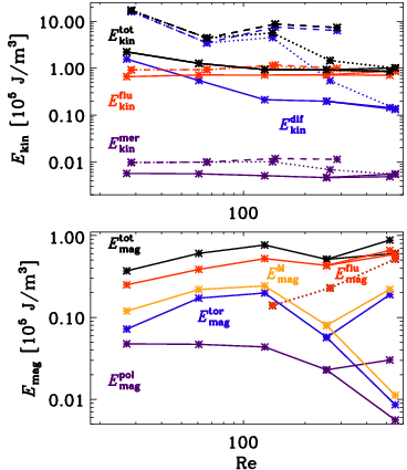
Figure 4: Dependence of kinetic and magnetic energies on Reynolds number Re. In the top panel we show the total kinetic energy $E_{\rm kin}^{\rm tot}$ (black), which is composed of the energy of the fluctuating flow $E_{\rm kin}^{\rm flu}$ (red), the differential rotation $E_{\rm kin}^{\rm dif}$ (blue), and the meridional circulation $E_{\rm kin}^{\rm mer}$ (purple) for H runs (dashed), M runs (solid) and S runs (dotted). Bottom: total magnetic energy density $E_{\rm mag}^{\rm tot}$ (black) composed of the energy densities of the fluctuating magnetic field $E_{\rm mag}^{\rm flu}$ (red), the mean toroidal $E_{\rm mag}^{\rm tor}$ (blue), and mean poloidal magnetic field $E_{\rm mag}^{\rm pol}$ (purple). $E_{\rm mag}^{\rm M}=E_{\rm mag}^{\rm tor}+E_{\rm mag}^{\rm pol}$ is the energy density of the mean magnetic field (yellow); see Equations (8)–(11) for definitions. The lower mean-field energy densities for $\mbox{\rm Re}\sim 530$ indicate Run 4M2, which has been started from Run S4 and is possibly not yet saturated, hence the bifurcation.

3.2 Energies

Next we look at the total (volume-averaged) energy densities as shown in Fig. 4 and Table 2. For the H runs, the kinetic energy is generally higher than for the other sets, and it is dominated by the differential rotation at all Reynolds numbers. For the M runs, the contribution of the differential rotation becomes weaker and sub-dominant w.r.t the velocity fluctuations with increasing Reynolds numbers. For the lowest diffusivities investigated, however, the contribution of differential rotation to the total kinetic energy seems to level off at a value of roughly 15%. The contribution of the meridional circulation is tiny for all runs. The energies of the fluctuating velocities remain for all sets roughly constant at increasing Reynolds numbers being, however, a bit higher for the H runs than for the M runs.

The S runs with small Re show similar dominance of differential rotation, but its contribution diminishes for growing Re similarly to the M runs. The S runs show basically a transition from an almost purely hydrodynamic state (2S) to a fully magnetically dominated state (4S). This has to be attributed to the SSD, strengthening strongly with growing Reynolds numbers, as will be discussed next.

The magnetic energy increases with increasing Re for the first three M runs. This is mostly due to the increase of the mean field. For higher Re, the energy in the mean field actually decreases, whereas the contribution of the small-scale field increases. The results for the lowest diffusivities (4M, 4M2) need to be taken with caution: Run 4M has been restarted from a remeshed earlier stage of 3M, at which the mean-field energy was still high, see Fig. 13 and its discussion in Section 3.6. Run 4M was most likely not run long enough to let the magnetic field reach a new saturated stage. For 3M, it took already $\sim\!10\leavevmode\nobreak\ {\rm yr}$ to saturate. Run 4M2 has been started from 4S to see how fast the mean field can recover after it has been removed. After running for $\sim\!0.06\leavevmode\nobreak\ {\rm yr}$, the mean field was still very weak.

For all runs, the mean field is dominated by its toroidal part. For all M runs, the small-scale field contribution dominates the total magnetic energy and shows some tendency to increase for high Re. In the runs without SSD (0M and 1M), the fluctuations contribute by roughly 65% to the total magnetic energy. When the SSD starts operating, this contribution increases from 68% (Run 2M) to 75% (4M).

In the S runs, we observe a significant increase of the magnitude of the magnetic fluctuations due to the strengthening SSD. Let us assume that $E_{\rm mag}^{\rm flu}$ in the S runs gives a good representation of the strength of the SSD-generated field also in the corresponding M runs, despite some differences in the flow dynamics. Then for $\mbox{\rm Re}\sim 130$ a quarter of $E_{\rm mag}^{\rm flu}$ is due to the SSD, increasing to nearly 80% for $\mbox{\rm Re}\sim 500$.

In our interpretation, at low Re, the quenching of the differential rotation is caused by the small-scale field generated by the tangling of the large-scale magnetic field, rather than by the large-scale field directly. At higher Re, the SSD also generates small-scale field, leading to a further quenching of the differential rotation.

If we do not consider Run 4M, given the issues mentioned above, the total magnetic field energy tends to saturate at high $\mbox{\rm Re}_{\rm M}$ because the increase in the fluctuating-field energy compensates for the decrease in the mean-field magnetic energy. This is in contrast to previous studies (Nelson et al. 2013; Hotta et al. 2016; Käpylä et al. 2017a), where the total field shows a steady increase with $\mbox{\rm Re}_{\rm M}$. However, as far as the mean field is concerned, our study is roughly consistent with the results of Nelson et al. (2013) and Hotta et al. (2016) as these authors find that the mean-field energy decreases with $\mbox{\rm Re}_{\rm M}$; yet, our study is inconsistent with our previous work (Käpylä et al. 2017a), where the mean field does not decrease.

The total magnetic energy is close to equipartition with the total kinetic energy only at the highest Re (4M) due to the strong mean-field and its tangled fluctuating field, see last two columns of Table 2. In the pure SSD runs, the field reaches only 50% of the equipartition value. This does not agree with the results of HKS22, where super-equipartition fields were found at their highest resolution.

3.3 Overshoot and Deardorff layers

Similar as in the work of Käpylä et al. (2019) and Viviani & Käpylä (2021) we found that using a Kramers-based heat conductivity causes the development of sub-adiabatic, yet convective layers in addition to the usual convective zone. From top to bottom of the domain, the zones are defined as

$$\overline{F}_{\rm enth}>0 \text{,}\quad{\rm d}{}s/{\rm d}{}r<0\quad$$ buoyancy zone (BZ) (12)

$$\overline{F}_{\rm enth}>0 \text{,}\quad{\rm d}{}s/{\rm d}{}r>0\quad$$ Deardorff zone (DZ) (13)

$$\overline{F}_{\rm enth}<0 \text{,}\quad{\rm d}{}s/{\rm d}{}r>0\quad$$ overshoot zone (OZ) (14)

$$\overline{F}_{\rm enth}<0 \text{,}\quad\left|\overline{F}_{\rm enth}\right|<0.03\overline{F}_{\rm tot}\quad \text{radiative zone (RZ)},$$ (15)

where $\overline{F}_{\rm enth}=c_{\rm P}\overline{(\rho u_{r})^{\prime}T^{\prime}}$ is the radial enthalpy flux, and $\overline{F}_{\rm tot}=\overline{F}^{\,\rm rad}(r=0.7\,R)$ is the total flux, defined by the flux through the bottom boundary. In the definitions above, all the fluxes are additionally averaged over latitude, hence they only depend on radius $r$.

We investigate the dependence of these zones on Re for different runs in Fig. 5. As a first result, we observe that approximately the lower quarter of the domain is convectively stable (even more so for low Re), consistent with previous works in similar parameter regimes (Käpylä et al. 2019; Viviani & Käpylä 2021).

The Deardorff zone is more pronounced near the equator in the high-diffusivity runs runs, especially in hydro cases. As Re increases, the Deardorff zones become narrower near the equator and more uniform over latitude, while their radial extent at high latitudes depends on the presence of magnetic fields. In the M Runs, the DZ becomes very thin and is partly replaced by a thin overshoot layer and an extended radiative zone for high Re. In the S Runs, the DZ is more pronounced at low latitudes, even at high Re. For the H Runs, it is always pronounced at low latitudes; however, at high Re, most of it is replaced by the overshoot zone. We attribute these extensions of the non-convective zones at low latitudes to the presence of strong differential rotation in the H runs, absent in the high Re M runs.

Regarding the discussion on how the depth of the OZ depends on Re (see Hotta 2017; Käpylä 2019c) our conclusion is complex. For all runs, at high latitudes the depth seems to remain rather constant, in agreement with Käpylä (2019c, 2021). However, at low latitudes, the depth decreases with Re for the H runs, aligning with Hotta (2017), but increases in the S runs. As for the depth of the DZ, Käpylä (2021) find a weak dependence on Re, which we can confirm for high latitudes but not throughout.

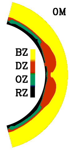
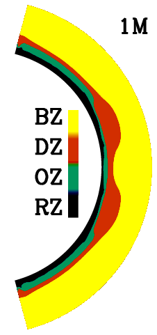
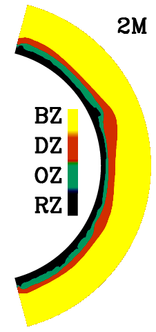
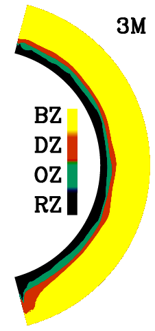
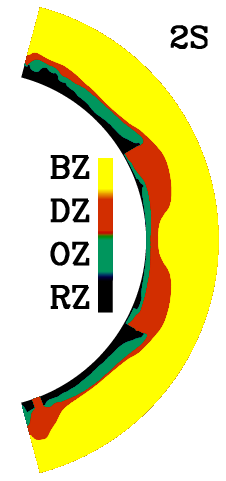
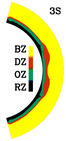
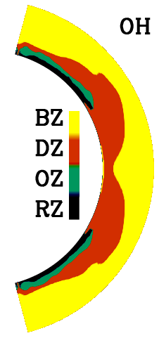
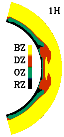
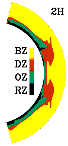
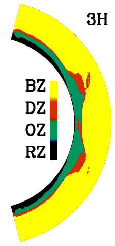
Figure 5: Visualization of the four zones formed in the simulations: buoyancy (BZ, yellow), Deardorff (DZ, red), overshoot (OZ, green), and radiative zone (RZ, dark blue), see Section 3.3 for definitions.

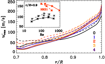
Figure 6: Radial profile of latitudinally averaged turbulent velocity $u^{\prime}_{\rm rms}$ of all runs. Colors indicate the different run sets with different Re as indicated. Solid lines, M runs, dotted S runs, dashed H runs. The inset shows $u^{\prime}_{\rm rms}$ at a fixed radius $r=0.9\,R$ as function of Re. There we overplot $u^{\prime}_{\rm rms}$ of Hotta & Kusano (2021) using Re estimated in HKS22 (solid red) and a re-estimate according to Equation (16) (dashed).

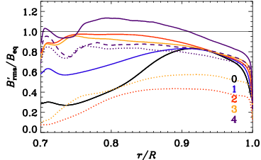
Figure 7: Radial profile of the normalized latitudinally averaged turbulent magnetic field $B^{\prime}_{\rm rms}/B_{\rm eq}$ of all runs. Color coding and line style as in Fig. 6, with the exception of Run 4M2 (dashed purple).

3.4 Flow and magnetic field distribution

The variation of the fluid and magnetic Reynolds numbers also impacts the distribution of turbulent velocity and magnetic fields. In Fig. 6, we illustrate the latitudinally averaged radial profiles of $u^{\prime}_{\rm rms}$ for all runs. Firstly, the values are somewhat lower than those expected for the Sun when relying on mixing length theory (Stix 2002). This deviation is expected due to the stronger rotational effects present in our simulations, as indicated by the Coriolis numbers ranging from $\mbox{\rm Co}=8$ to $9$. Near the surface, significant discrepancies arise, likely due to the absence of a strong density stratification. The M runs show the poorest agreement, while the H runs exhibit higher velocities compared to their M counterparts. The S runs fall between these two. We interpret this as turbulent velocities being suppressed by the presence of magnetic fields, primarily by the large-scale one.

Upon investigating turbulent velocity as a function of Re (see inset in Fig. 6), we observe that for all H runs, $u^{\prime}_{\rm rms}$ is larger than for the M runs, with the S runs consistently in between. Velocity fluctuations increase for all run sets initially with Re and then decrease for higher Re; however, this decrease is not as pronounced as the initial increase. The decrease in $u^{\prime}_{\rm rms}$ in Run 4M might be caused by the magnetic field, but we observe a mild decrease in Run 3H, too, and even an increase for Run 4S. Therefore, this interpretation may not be entirely accurate.

We also compare our velocities to the results of HK21, who find that the SSD suppresses the turbulent velocity as their effective Re increases. Since they do not explicitly define Re due to the usage of a slope-limited diffusion (SLD) scheme without explicit diffusivities, they estimate Re using the Taylor microscale. As an alternative, we estimate their Re using the grid spacing of our Set 4:

$$\mbox{\rm Re}_{\rm HK21}=\mbox{\rm Re}_{\rm 4}\Delta\phi_{\rm 4}/\Delta\phi_{\rm HK21}.$$ (16)

Here, $\mbox{\rm Re}_{\rm 4}=530$ is a rough average of all Re in Set 4, $\Delta\phi_{\rm 4}=\pi/2/2048$ the grid size in this set, and $\Delta\phi_{\rm HK22}=2\pi/(1536,3072,6144)$ the variable grid size of the three runs of HK21. This approach ensures that Re does not increase much more than by a factor of two when the resolution is doubled, in contrast to the approach of HKS22.

Comparison reveals two significant findings: Firstly, as evident from the inset of Fig. 6, their $u^{\prime}_{\rm rms}$ values are markedly higher than ours and exceed those of a typical solar model (Stix 2002). This implies that the model proposed by HK21 does not adequately represent the Sun, particularly in terms of turbulent velocities. Secondly, our simulations do not exhibit a decrease in $u^{\prime}_{\rm rms}$ with increasing Re, as as notable as observed in HK21; instead, we observe only a mild decrease at high Re. Two explanations for this behavior can be considered: Firstly, it may be linked to the more efficient SSD in HK21’s highest resolution simulation, likely a result of higher turbulent velocities. Secondly, it could be a consequence of their use of a pure SLD scheme for viscous and magnetic diffusion, as opposed to the constant explicit diffusivities employed in our study. This is supported by the fact that HK21 achieves a more efficient SSD at an even lower resolution than we do.

However, if the turbulent velocities were quenched by the SSD at high Re, we would expect to see a suppression of $u^{\prime}_{\rm rms}$ as a function of Re only for M and S runs, yet we also observe it for H runs. Another possible cause may be the specific setup of HK21, where the energy fluxes are fixed to the solar luminosity at both radial boundaries, forcing the total energy to remain constant at its initial value. With such a constraint, an increase in kinetic energy due to higher Re and Ra might not be as straightforward as in our configuration: A strong SSD has to transform turbulent kinetic to magnetic energy efficiently. However, because turbulent kinetic energy is not easily replenished, it has to decrease. However, this depends on how efficiently convection can transform stored thermal energy into kinetic energy in both setups. Further numerical investigations are required to explore this issue. Presently, we are confident that our model, allowing thermal energy to adjust to the dynamics, is more self-consistent and hence more realistic.

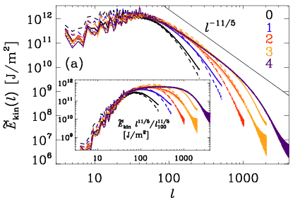
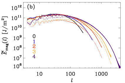
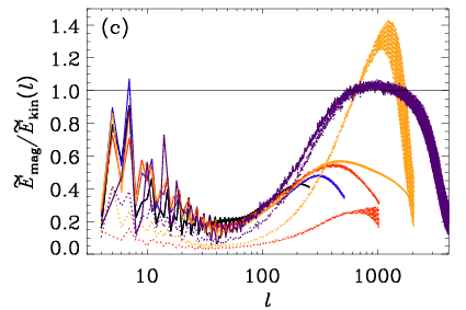
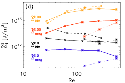
Figure 8: Spectra of kinetic (a) and magnetic (b) energy along with their ratio (c) near the surface, $r=0.98\,R$, all excluding the $m=0$ contribution. As before: M runs - solid, S runs - dotted, H runs - dashed lines, while different colors indicate run sets with distinct Re. Panel (d) highlights the Re dependence of kinetic and magnetic spectra for $l=10$ and $100$.

Next, we examine the latitudinally averaged turbulent magnetic field strength $B^{\prime}_{\rm rms}$, normalized by the equipartition field strength (see Fig. 6 for the turbulent kinetic energy). As expected, the turbulent magnetic field increases with Re for the M and S runs. Weak super-equipartition fields are observed only for Run 4M in the middle of the convection zone. Runs 4M2, 4S, 3M, and 2M reach values above $B^{\prime}_{\rm rms}/B_{\rm eq}=0.9$ but do not exceed unity in the entire convection zone. The pure SSD (S) runs consistently exhibit weaker $B^{\prime}_{\rm rms}$ compared to their M counterparts.

Interestingly, the field increases with $\mbox{\rm Re}\,(=\!\mbox{\rm Re}_{\rm M})$ for the M runs, mostly in the lower half of the convection zone, and appears mostly independent of $\mbox{\rm Re}_{\rm M}$ in the upper part of the domain. Only the highest $\mbox{\rm Re}_{\rm M}$ run (4M) shows a slightly enhanced field in the upper part of the domain. In contrast, the S runs show an increase of $B^{\prime}_{\rm rms}$ with $\mbox{\rm Re}_{\rm M}$ throughout the domain. We interpret this as follows: In the M runs, where the SSD is still weak, $B^{\prime}_{\rm rms}$ is primarily generated by the tangling of the large-scale magnetic field. This process seems independent of Re for the upper part of the domain while becoming more effective in the lower part of the domain as Re increases. As the SSD increases similarly at all radii, it also enhances $B^{\prime}_{\rm rms}$ for the highest Re runs, where the SSD field becomes comparable to the tangled one.

In Fig. 8, we present the spherical-harmonic spectra of kinematic and magnetic energies along with their ratio for all runs, calculated from near the surface ($r=r_{s}\equiv 0.98\,R$) $\theta\phi$-slices. The spectral energies $\tilde{E}_{\rm kin}(l)$ and $\tilde{E}_{\rm mag}(l)$ are calculated using the following definitions:

$$\sum_{l}\tilde{E}_{\rm kin}(l)=r_{s}\left.E_{\rm kin}\right|_{r=r_{s}}\quad\sum_{l}\tilde{E}_{\rm mag}(l)=r_{s}\left.E_{\rm mag}\right|_{r=r_{s}},$$ (17)

where $l$ is the spherical-harmonic degree, and the energy densities are given as

$$\left.E_{\rm kin}\right|_{r=r_{s}}={\textstyle{1\over 2}}\left.\langle\rho\mbox{\boldmath$u$}{}^{\prime 2}\rangle_{\theta\phi}\right|_{r=r_{s}}\quad\left.E_{\rm mag}\right|_{r=r_{s}}={\textstyle{1\over 2}}\left.\langle\mbox{\boldmath$b$}{}^{\prime 2}\rangle_{\theta\phi}\right|_{r=r_{s}}.$$ (18)

We have removed the mean-field contribution ($m=0$) and summed over all other $m$. Because of our “wedge” approach, $l=4$ is the lowest possible $l$. See Viviani et al. (2018) and Käpylä et al. (2019) for details on how to compute spherical harmonic decompositions from simulations of the presented type.

For low $l$, the kinetic energy spectra (Fig. 8a) are similar for all runs, with only the hydro runs having slightly higher energies. At the highest resolutions and $l>50$, the velocity develops an inertial range, which can be best described by a power-law of $l^{-11/5}$, illustrated by the compensated spectrum in the inset. Such a power-law has been predicted by Bolgiano (1959) and Oboukhov (1959), and also found in Käpylä (2021). However, as discussed in several studies (e.g., Brandenburg 1992; Rieutord & Rincon 2010; Xie & Huang 2022; Alam et al. 2023), this scaling was obtained for stably stratified media but not for rotating convection. Also, the Bogliani-Obukhov scaling should appear only for those larger scales, which are influenced by the gravity-induced anisotropy, while being followed by a standard Kolmogorov scaling for smaller scales. Furthermore, we observe an extended inertial range only at the highest resolutions, as viscous diffusion affects all $l$ otherwise.

For the magnetic spectra (Fig. 8b), the energies are at low $l$ very similar for all M runs; only 4M has lower power at $l<10$, which might be caused by some data loss. We do not observe an inertial range with a clear power law as in the H runs. For the S runs, the energies are lower at all scales compared to the corresponding M runs. Yet, Run 4S has higher power than the other S runs, in particular at low $l$, while seeming indistinguishable from Run 4M for $l>100$. The field in the S runs being lower than in the M runs, in particular at low l, is consistent with nearly all the field at $l>500$ being due to the SSD, whereas tangling is dominant at $l<500$ for the highest $\mbox{\rm Re}_{\rm M}$. Surprisingly, we find no significant difference between the shape of the spectra of the M and S runs, implying that the spectral properties of LSD- and SSD-generated fields are very similar, at least for $l\geq 4$. We only observe that amplitude differences are more pronounced at $l<100$.

To investigate whether the magnetic field reaches super-equipartition at certain scales, we also examine the ratio of the magnetic and kinetic spectra near the surface, as shown in Fig. 8c. Only in Run 3S, super-equipartition is achieved (around $l\sim 1000$), whereas the corresponding M run has a maximum ratio of 0.6. The lowest diffusivity runs only achieve just equipartition for $600<l<2000$. It should be stressed that these spectra are taken close to the surface, where the horizontally averaged magnetic field is well below equipartition, as seen in Fig. 7. We would expect the spectral ratio at larger depths to be higher. The fanning of the spectra, particularly at high $l$ in the kinetic ones, is related to inaccuracies resulting from employing spherical harmonic decomposition on a spherical grid with incomplete $\theta$ range.

To show more clearly the Re dependence of the spectral energy, we plot for $l=10$ and $100$ the kinetic and magnetic energy as function of Re for all runs, see Fig. 8d. We find that the kinetic energy for $l=10$ seems to decrease mildly with increasing Re, interestingly not only for M or S runs, but also for H runs, hence this cannot be due to a suppression by the magnetic field as claimed in HK21. The magnetic energy at $l=10$ of the M runs seems to be independent of Re, except a mild decrease for the highest Re. Only for the S runs, we see a strong increase. For the kinetic and magnetic energy at $l=100$, we find a continuous increase. Only the kinetic energy seems to saturate for the highest Re. For this scale, we do not find that the strong SSD in the highest Re runs has a marked influence on the kinetic energies.

If we compare our results with the spectra provided by HK21 and HKS22, we find two main differences: The authors observe super-equipartition fields at small scales ($l>100$) even for their lowest resolution (similar to our Set 2). Additionally, in their work the kinetic energy in large scales becomes suppressed at high Re because of, as they interpret it, their very strong SSD. We observe a small decrease in the large-scale energy, but this is also evident in the hydrodynamic runs. It is important to note that in HK21 and HKS22, only one pure hydrodynamic run is studied; therefore there is no Re dependence in their case. Furthermore, their simulations only develop an SSD but no LSD; hence, the influence of a large-scale field on the dynamics was not studied. The differences in the spectral properties might also be related to these two main distinctions in the setup as discussed above.

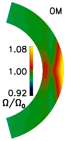
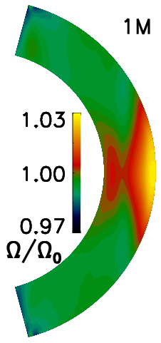
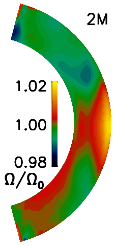
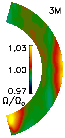
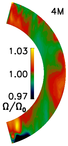
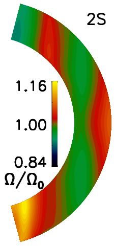
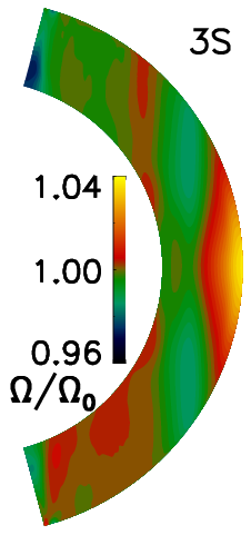
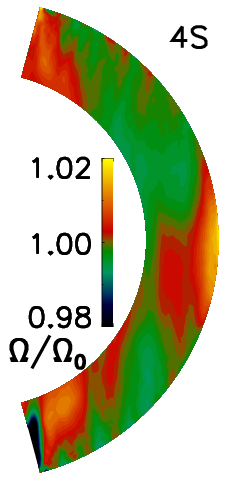
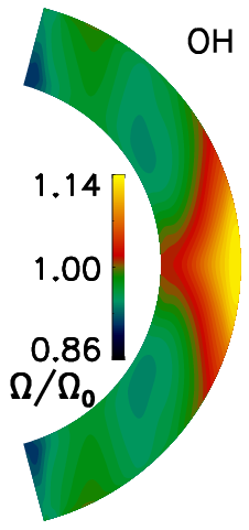
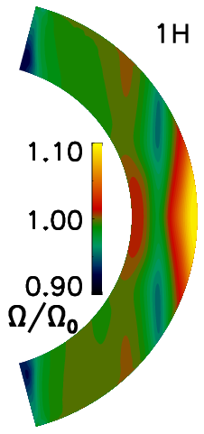
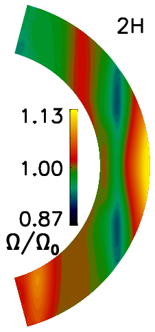
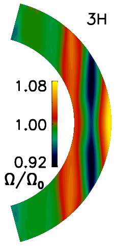
Figure 9: Differential rotation $\Omega/\Omega_{0}$, with $\Omega=\Omega_{0}+\overline{u}_{\phi}/r\sin\theta$ for all runs.

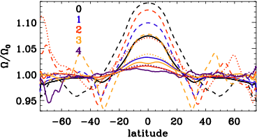
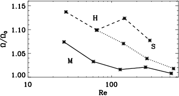
Figure 10: Differential rotation of all runs near the surface ($r=0.98\,R$). Top: $\Omega/\Omega_{0}$ as function of latitude. As before, M runs - solid, S runs - dotted, H runs - dashed lines, and colors indicate the run sets with different Re. Bottom: $\Omega/\Omega_{0}$ at the equator ($\theta=\pi/2$) as function of Re.

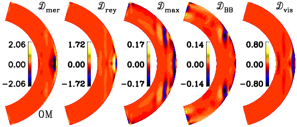
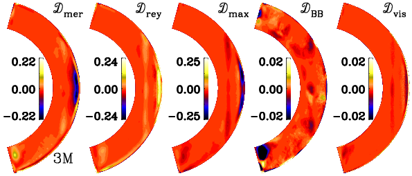
Figure 11: Time-averaged contributions to the differential rotation energy evolution for Runs 0M and 3M, as given in Equations (21)–(25). The contributions are shown in units of J/m³s.

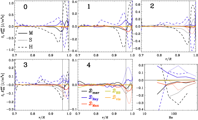
Figure 12: Contributions to differential rotation energy evolution averaged in time and latitude for all run sets as functions of $r/R$, see Equations (21)–(25). The rightmost bottom panel shows the contributions as functions of Re at $r/R$=0.96 (vertical line in othe rpanels).

3.5 Differential rotation and its generators

Next, we examine the profiles of differential rotation $\Omega=\Omega_{0}+\overline{u}_{\phi}/r\sin\theta$ as shown in Figs. 9 and 10, and investigate the influence of the magnetic fields on their generation terms, see Figs. 11 and 12. As observed from the energy analysis, the differential rotation is most pronounced in the H runs and suppressed in the M and S runs.

In the H runs, the contours of constant angular velocity tend to become more cylindrical towards the more turbulent regime, while the maximum $\Omega$ values remain roughly constant across Runs 0H, 1H, and 2H. However, for the highest Re (Run 3H), the differential rotation is slightly weaker compared to Run 1H. With increasing Re, more jets of opposite signs become visible. Surprisingly, in Run 0H the contours are far less cylindrical compared to the H runs with higher Re. We attribute this to the absence of Busse columns (or banana cells) at the lowest Re, as illustrated in Fig. 21.

As previously noted, the M runs consistently exhibit weaker differential rotation, with their $\Omega$ profiles being strongly influenced by the magnetic field. We observe a tendency for the isorotation contours to become less cylindrical with higher Re. Excluding some local minima and maxima near the poles, the differential rotation becomes much weaker in the highly turbulent regime compared to the less turbulent one. Additionally, in all cases with active SSD, the differential rotation profile becomes increasingly hemispherically asymmetric with rising Re, attributable to the hemispherically asymmetric magnetic field. Notably, the minimum of $\Omega$ at mid-latitudes nearly vanishes in the high-Re M runs. For the S runs, the profiles at weak SSD (Run 2S) resemble those of Run 2H. However, Run 3S with stronger SSD exhibits weaker differential rotation, akin to Run 3M. Comparing the profiles of Run 4S and 4M reveals hardly any differences. This might be related to the issues of these runs discussed in Section 3.2.

The changes in the differential profile with Re and the presence of the two dynamos become clearer in the plots of latitudinal distribution and Re dependence (Fig. 10) of $\Omega$. It is evident that it significantly decreases near the equator with increasing Re and in the presence of a magnetic field. Moreover, the jets present in the H runs at mid-latitudes are completely suppressed in the M runs. Interestingly, the differential rotation at the equator is already strongly suppressed in Run 2M, where the SSD is relatively weak, indicating that the suppression is due to the magnetic field generated by the LSD rather than the SSD. However, the SSD in Run 4S is capable of suppressing and shaping the differential rotation similarly to its corresponding Run 4M.

The reduction of shear at high $\mbox{\rm Re}_{\rm M}$ has also been reported by Käpylä et al. (2017a). HK21 and HKS22 find that at high $\mbox{\rm Re}_{\rm M}$, the differential rotation is also strongly influenced by the magnetic field, which is consistent with our work. However, in their cases, the magnetic field is solely due to an SSD, whereas in our case, the change in differential rotation is mainly due to the LSD.

Our modelling strategy does not allow us to inspect the actual generation process of the differential rotation profiles, as we re-start from earlier models. Hence we can only address reliably the relaxed states.

The differential rotation follows the mean angular momentum balance (see, e.g. Rüdiger 1989),

$${\partial_{t}}\left(s^{2}\overline{\rho}\Omega\right)=-\mbox{\boldmath$\nabla$}{}\cdot s \left[s\overline{\rho\mbox{\boldmath$u$}{}}\Omega+\overline{\left(\rho\mbox{\boldmath$u$}{}\right)^{\prime}u^{\prime}_{\phi}}-2\nu\overline{\rho}\overline{}\mbox{\boldmath${\sf S}$}{}\cdot\hat{\mbox{\boldmath$e$}}{}_{\phi}\right.$$

$$\left.-\mu_{0}^{-1}\left(\overline{\mbox{\boldmath$B$}}{}\,\overline{B}_{\phi}+\overline{\mbox{\boldmath$B$}{}^{\prime}B_{\phi}^{\prime}}\right)\right],$$ (19)

where $s=r\sin\theta$ is the lever arm. As usual, we neglect the compressible term related to $\overline{\rho^{\prime}\mbox{\boldmath${\sf S}$}{}^{\prime}}$ in the equation above.

To check which part of the angular momentum flux contributes significantly to the differential rotation, we calculate the contributions to the evolution of differential rotation energy density. This approach has the advantage that generating contributions are shown as positive values, and destructing ones as negative.

$${\partial_{t}}E^{\rm diff}_{\rm kin}=(\overline{u}_{\phi}/s)\partial_{t}\left(s^{2}\overline{\rho}\Omega\right)={\textstyle{1\over 2}}\partial_{t}(\overline{\rho}\,\overline{u}_{\phi}^{2})=\cal{D},$$ (20)

Using the right hand side of Equation (19), we can divide $\cal{D}$ into five different contributions

$$\cal{D}_{\rm Mer} = - \,(\overline{u}_{\phi}/s)\,\mbox{\boldmath$\nabla$}{}\cdot\left(s^{2}\overline{\rho\mbox{\boldmath$u$}{}}\Omega\right)$$ meridional circulation, (21)

$$\cal{D}_{\rm Rey} = - \,(\overline{u}_{\phi}/s)\,\mbox{\boldmath$\nabla$}{}\cdot\left(s\overline{\left(\rho\mbox{\boldmath$u$}{}\right)^{\prime}u_{\phi}^{\prime}}\right)$$ Reynolds stress, (22)

$$\cal{D}_{\rm Max} = \,(\overline{u}_{\phi}/s)\,\mbox{\boldmath$\nabla$}{}\cdot\left(s\mu_{0}^{-1}\overline{\mbox{\boldmath$B$}{}^{\prime}B_{\phi}^{\prime}}\right)$$ SS Maxwell stress, (23)

$$\cal{D}_{\rm BB} = \,(\overline{u}_{\phi}/s)\,\mbox{\boldmath$\nabla$}{}\cdot\left(s\mu_{0}^{-1}\overline{\mbox{\boldmath$B$}}{}\,\overline{B}_{\phi}\right)$$ LS Maxwell stress, (24)

$$\cal{D}_{\rm vis} = \,(\overline{u}_{\phi}/s)\,\mbox{\boldmath$\nabla$}{}\cdot\left(2s\nu\overline{\rho}\overline{}\mbox{\boldmath${\sf S}$}{}\cdot\hat{\mbox{\boldmath$e$}}{}_{\phi}\right)$$ viscous stress. (25)

Due to our choice of azimuthal averages written out during run time, we calculate $\cal{D}_{\rm Mer}$ and $\cal{D}_{\rm Rey}$ slightly differently. However, their sum will be the same. For $\cal{D}_{\rm Mer}$, we use

$$\mbox{\boldmath$\nabla$}{}\cdot\left(s^{2}\overline{\rho\mbox{\boldmath$u$}{}}\Omega\right)\approx\mbox{\boldmath$\nabla$}{}\cdot\left(s^{2}\overline{\rho}\,\overline{\mbox{\boldmath$u$}}{}\,\Omega\right)+\mbox{\boldmath$\nabla$}{}\cdot\left(s^{2}\overline{\rho^{\prime}\mbox{\boldmath$u$}{}^{\prime}}\Omega_{0}\right),$$ (26)

where the second term is calculated by $-s^{2}\Omega_{0}\mbox{\boldmath$\nabla$}{}\cdot\left(\overline{\rho}\,\overline{\mbox{\boldmath$u$}}{}\right)$ using the conservation of mass flux

$$\mbox{\boldmath$\nabla$}{}\cdot\left({\rho\mbox{\boldmath$u$}{}}\right)=\mbox{\boldmath$\nabla$}{}\cdot\left(\overline{\rho^{\prime}\mbox{\boldmath$u$}{}^{\prime}}\right)+\mbox{\boldmath$\nabla$}{}\cdot\left(\overline{\rho}\,\overline{\mbox{\boldmath$u$}}{}\right)=0\,.$$ (27)

For $\cal{D}_{\rm Rey}$ we use

$$\mbox{\boldmath$\nabla$}{}\cdot\left(s\overline{\left(\rho\mbox{\boldmath$u$}{}\right)^{\prime}u_{\phi}^{\prime}}\right)\approx\mbox{\boldmath$\nabla$}{}\cdot\left(s\overline{\rho\mbox{\boldmath$u$}{}u_{\phi}}\right)-\mbox{\boldmath$\nabla$}{}\cdot\left(s\overline{\rho}\,\overline{\mbox{\boldmath$u$}}{}\,\overline{U}_{\phi}\right).$$ (28)

Our choice at the end means that the term $\mbox{\boldmath$\nabla$}{}\cdot\left(s\,\overline{\rho^{\prime}\mbox{\boldmath$u$}{}^{\prime}}\,\overline{U}_{\phi}\right)$ is included in $\cal{D}_{\rm Rey}$ instead of in $\cal{D}_{\rm Mer}$, hence their sum is the same as in the definitions Equations (21) and (22).

We show the time-averaged contributions exemplarily for Runs 0M and 3M as a meridional plot in Fig. 11 and for all runs as a line plot from additional averaging over latitude in Fig. 12. For all low Re runs, the main balance is between the contributions of meridional circulation $\cal{D}_{\rm mer}$ and Reynolds stresses $\cal{D}_{\rm Rey}$ with a small contribution of $\cal{D}_{\rm vis}$. For most of the domain, $\cal{D}_{\rm Rey}$ is generative whereas $\cal{D}_{\rm mer}$ is destructive. At high Re, this balance still holds for the H runs, where $\cal{D}_{\rm vis}$ becomes increasingly smaller. For the M runs, we find two main channels through which the magnetic field influences the angular momentum. On one hand, the magnetic field suppresses $\cal{D}_{\rm mer}$ and $\cal{D}_{\rm Rey}$ to much lower levels, accompanied by some changes in the spatial distribution. On the other hand, the contribution from small-scale Maxwell stresses $\cal{D}_{\rm Max}$ becomes comparable to $\cal{D}_{\rm Rey}$, but has mostly negative values, hence compensating $\cal{D}_{\rm Rey}$. Surprisingly, this happens already at $\mbox{\rm Re}\sim 60$, where no SSD is present. The direct influence of the large-scale magnetic field ($\cal{D}_{\rm BB}$) appears to be significant only near the surface at high Re, where it has a destructive effect. For the S runs, we find that the contribution of $\cal{D}_{\rm Rey}$ is not as effectively quenched as in the corresponding M runs. The magnetic influence primarily comes through the $\cal{D}_{\rm Max}$ contribution, which has a destructive effect across most of the convection zone. Together with the destructive contribution of $\cal{D}_{\rm mer}$, it balances $\cal{D}_{\rm Rey}$.

From this differential rotation energy balance, we can deduce the reason why the differential rotation is mostly quenched by the presence of the LSD rather than the SSD alone. The quenching of $\cal{D}_{\rm Rey}$ appears to play an important role here. Only the large-scale field can effectively quench this contribution, preventing the development of strong differential rotation. Additionally, the small-scale magnetic field, whether generated by tangling or by an SSD, creates a destructive term, $\cal{D}_{\rm Max}$, which further suppresses the generation of differential rotation.

In theory, Maxwell stresses could also act similarly to Reynolds stresses in generating differential rotation; however, we find that their contribution is always destructive. Previous studies by Käpylä et al. (2017a) have shown that the contribution of the Reynolds stress is balanced by the contribution of meridional circulation, and that this balance shifts to a balance of Reynolds and Maxwell stress contributions. This finding has been confirmed by HK21 and HKS22. However, the latter authors mostly attribute this change in balance to the presence of an SSD, whereas we find that this is already the case at moderate $\mbox{\rm Re}_{\rm M}$, where no SSD is present. That large-scale magnetic fields suppress differential rotation via the quenching of the $\Lambda$ effect was studied intensively in mean-field models (e.g Kitchatinov et al. 1994b; Kitchatinov 2016; Pipin 2017) and also confirmed by numerical simulations (Käpylä 2019b). However, the magnetic field will also affect the turbulent viscosity in such mean-field models (e.g. Kitchatinov et al. 1994a), therefore differential rotation can also be enhanced (Kitchatinov 2016). Quenching of the $\Lambda$ effect by SSD has been found to be milder than by a corresponding large-scale magnetic field with the same strength using simplified numerical simulations (Käpylä 2019a).

The importance of Busse columns (or banana cells) for the generation of differential rotation has previously been pointed out by other authors (e.g Hotta et al. 2015; Featherstone & Hindman 2016; Matilsky et al. 2020; Bekki et al. 2022; Käpylä 2023). One of their interpretations is that the prominent presence of these large-scale convective structures in simulations makes the differential rotation of the Sun difficult to reproduce. Our results are in line with this interpretation, because the banana cells seem to make the differential rotation profile more cylindrical, whereas the contours of the Sun’s differential rotation are radial over a considerable range of mid-latitudes (e.g. Schou et al. 1998).

$B_{\phi}(r=0.98\,R)$	$B_{\phi}(r=0.71\,R)$	$B_{\phi}(\theta=25^{\circ})$

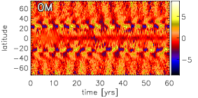
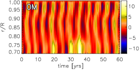
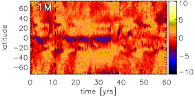
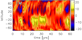
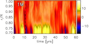
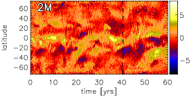
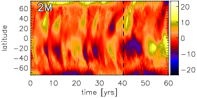
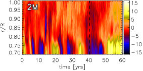
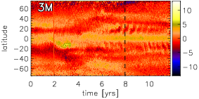
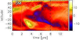
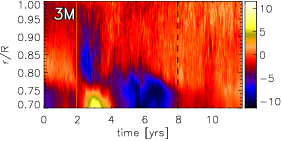
Figure 13: Time evolution of the mean toroidal magnetic field $\overline{B}_{\phi}$ for all M runs (except 4M and 4M2). We show time-latitude (butterfly) diagrams at $r=0.98\,R$ (first column), at $r=0.71\,R$ (second column) and the time-radius diagram at 25^∘ latitude (north). We note that the time scale for the first three rows are the same, but different for the last one. The vertical dashed lines indicate the starting point from which we use a time interval to compute time averages utilized in the analysis throughout this paper. Vertical stripes in Run 3M are due to data loss.

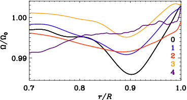
Figure 14: Radial profile of the differential rotation $\Omega/\Omega_{0}$ of all M runs. We show the radial profile at 25^∘ latitude, which coincide with the local minimum of $\Omega$ causing the equatorward migration magnetic field pattern in 0M.

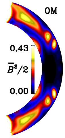
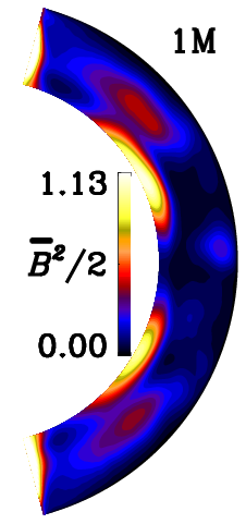
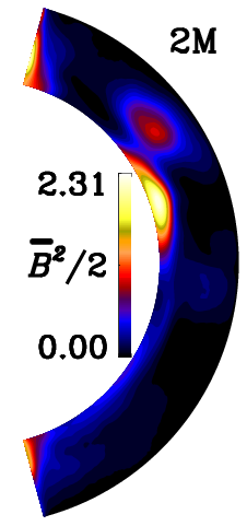
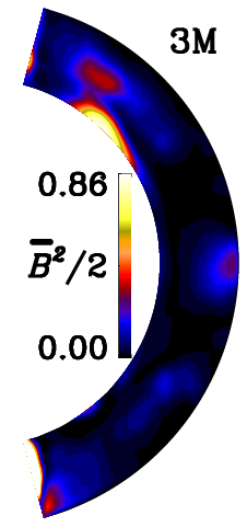
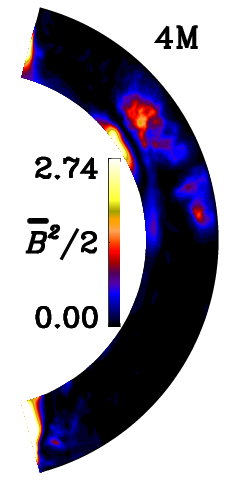
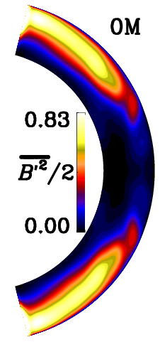
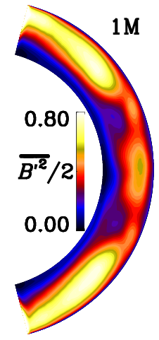
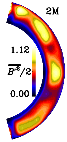
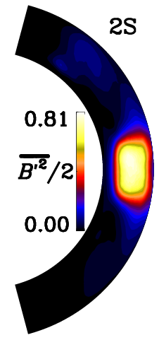
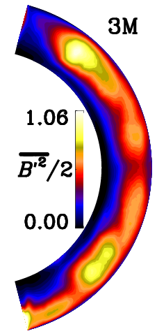
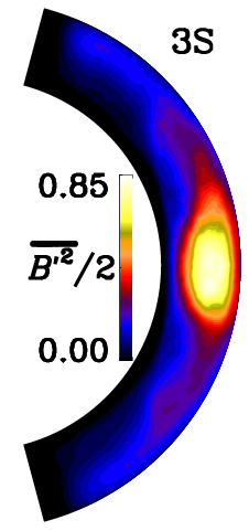
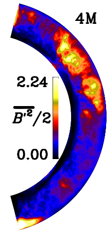
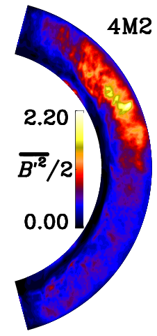
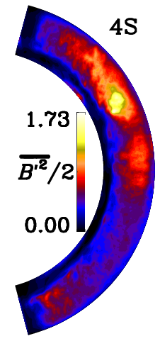
Figure 15: Time-averaged mean magnetic energy of the mean fields $\overline{\mbox{\boldmath$B$}}{}^{2}/2$ (top row) and fluctuating fields $\overline{\mbox{\boldmath$B$}{}^{\prime 2}}$ (bottom) for all M and S runs in the units of 10⁵ J/m³ for all magnetic runs (M+S). We disregard 7^∘ near the latitudinal boundary for determining the minimum and maximum values of the color range.

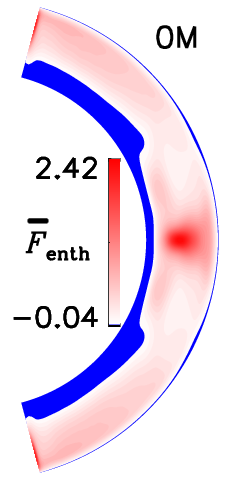
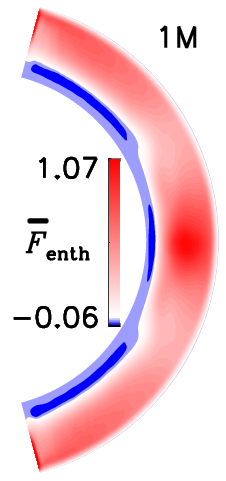
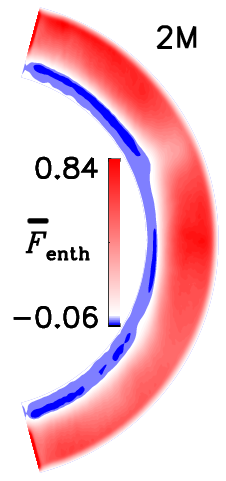
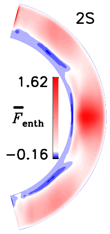
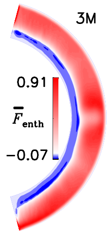
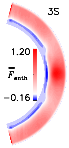
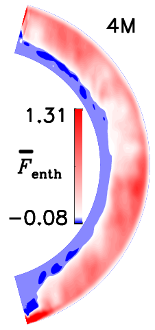
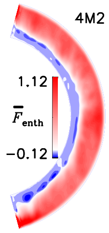
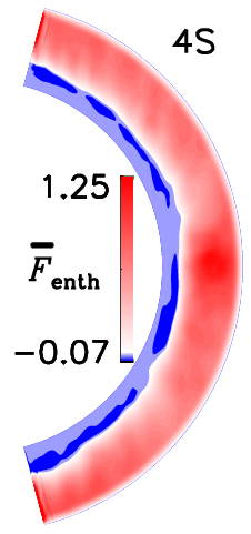
Figure 16: Time-averaged radial enthalpy flux $\overline{F}_{\rm enth}$ normalised by the input flux $\overline{F}_{\rm tot}$ for all magnetic runs (M+S). We neglect 7^∘ near the latitudinal boundary for determining the minimum and maximum values of the color range.

3.6 Magnetic field generation

Next, we look at the evolution of the mean toroidal magnetic field $\overline{B}_{\phi}$, plotting in Fig. 13 the butterfly diagrams of Runs 0M, 1M, 2M and 3M; for Run 4M, the time series is too short to form a meaningful diagram. Run 0M shows a very similar mean field evolution as the run of Käpylä et al. (2016): a regular cycle with equatorward migration throughout the convection zone, a fast cycle with poleward migration near the surface close to the equator and a long cycle most pronounced at the bottom of the domain, capable of disturbing the other cycles. This is expected as 0M has the same parameters as the run of Käpylä et al. (2016), except for the use of a Kramers-based heat conduction instead of a prescribed conductivity profile. The dynamo mode with equatorward migration, first reported in Käpylä et al. (2011a) and further discussed in Käpylä et al. (2013), can be clearly explained by an $\alpha\Omega$ Parker dynamo wave (e.g. Warnecke et al. 2014, 2018). However, to obtain the exact period, many other turbulent transport coefficients play a role (Warnecke et al. 2021). The fast poleward dynamo mode could be identified as being of $\alpha^{2}$ type (Käpylä et al. 2016; Warnecke et al. 2021), while the type of the long-period mode is currently not clear (Käpylä et al. 2016; Gent et al. 2017).

Increasing now Re and $\mbox{\rm Re}_{\rm M}$ influences the dynamo solutions: The clear equatorward migration vanishes for all runs starting from 1M. This is most likely due to changes in the differential rotation profile, see discussion below. The two other modes, however, still exist in the higher $\mbox{\rm Re}_{\rm M}$ regime. For the highest values of $\mbox{\rm Re}_{\rm M}$ (4M), the time series is unfortunately too short to identify the dynamo cycles safely. The fast dynamo mode is clearly visible also in the 1M, 2M and even the 3M run. That this mode is still visible also in Run 3M assures our interpretation as an $\alpha^{2}$ type dynamo because, as discussed in Section 3.5, the differential rotation becomes very weak at these high $\mbox{\rm Re}_{\rm M}$. The long-cycle dynamo mode is rather irregular and mostly pronounced in field strength, but it develops also polarity reversals. Comparing the butterfly diagrams of 1M and 2M, we find that they look very similar, in particular near the bottom of the domain and at higher latitudes. In summary, increasing the Reynolds numbers does not strongly affect the short and long cycles, still generating significant mean magnetic fields, but causes the equatorward migrating medium-length mode to vanish.

To investigate why this mode vanishes, we inspect in more detail the changes in the differential rotation profile roughly at the latitudinal and radial locations of generation of the previously found equatorward migrating dynamo mode, see Fig. 14. The minimum of $\Omega$ at $r=0.9$ and 25^∘ latitude is very pronounced in the 0M run, in 1M and 2M it is already much weaker, but in the run with the highest $\mbox{\rm Re}_{\rm M}$ (3M) it has vanished completely. This fits well with our hypothesis that the negative shear in this region generates the equatorward migrating dynamo mode seen in 0M (Warnecke et al. 2014, 2018); accordingly, when the shear is sufficiently weakend, this dynamo mode vanishes. To pinpoint which dynamo is actually working in these simulations, one needs to measure the turbulent transport coefficients as in Warnecke et al. (2018) and analyse them via a mean-field model as in Warnecke et al. (2021). Such an analysis is currently under development and will be presented in possible follow-up study.

To inspect at which locations the LSD and the SSD operate in our runs, we show in Fig. 15 meridional plots of azimuthally averaged magnetic energy density of the mean and fluctuating fields separately. We remind the reader that the magnetic fluctuations in Runs 0M and 1M are entirely generated by the tangling of the large-scale field, because in these runs no SSD is operating. In Run 0M, the large-scale field is mostly generated at mid- to high latitudes near the middle of the convection zone, which is consistent with earlier findings of runs with similar parameters (Warnecke et al. 2014, 2018; Käpylä et al. 2016). There is also a weaker field near the bottom of the domain, causing the long-term variation seen in Fig. 13. The corresponding small-scale field is located also at mid to high latitudes as one would expect from the large-scale field. However, near the bottom of the domain no small-scale field is generated, due to the weakness of the convective motions in this area, see Section 3.3. For the M runs with higher $\mbox{\rm Re}_{\rm M}$, the mean field at mid-latitudes gradually vanishes and instead becomes dominant near the bottom of the domain. The small-scale field is for small $\mbox{\rm Re}_{\rm M}$ mostly located at high latitudes, but gradually becomes stronger near the equator. This increase is partly due to tangling as in 1M, but in particular for higher $\mbox{\rm Re}_{\rm M}$ due to the SSD operating in this area, as seen from runs 2S and 3S. At the locations, where the small-scale field is strong, the enthalpy flux and the kinetic energy also reach a maximum, as shown in Fig. 16 for the enthalpy flux $\overline{F}_{\rm enth}$. Such a concentration of $\overline{F}_{\rm enth}$ near the equator was also observed in Käpylä et al. (2019) and Viviani & Käpylä (2021). We therefore believe that the maximum of the small-scale field in these areas is due to the enhanced convective motions. However, this is only true for the S runs. In the M runs, the situation is slightly different. In Run 2M, where already an SSD is present, we indeed see a concentration of small-scale field near the equator, similar to 2S, but also at higher latitudes, where the large-scale field is strong. The small-scale field seems still to be connected with the entropy flux, as the distribution of $\overline{{\mbox{\boldmath$B$}{}^{\prime}}^{2}}$ resembles the distribution of $\overline{F}_{\rm enth}$.

For the high-$\mbox{\rm Re}_{\rm M}$ runs (3M and 4M), the small-scale field is not concentrated near the equator as one would expect from their corresponding S runs. However, here too, the distribution of $\overline{{\mbox{\boldmath$B$}{}^{\prime}}^{2}}$ somewhat resembles the distribution of $\overline{F}_{\rm enth}$, at least in terms of a minimum near the equator.

Furthermore, even though the mean field is very strong near the bottom of the domain, the small-scale field is nearly zero. This is most likely due to the lack of strong convective motions there. We can explain the strong mean-field at the bottom with the possibility that the field is generated above and then transported down by turbulent pumping or diffusion and finally diffuses slowly into this nearly turbulent-free zone, where it can survive for a long time, because of the lack of strong turbulent diffusion. As another possibility, the field can be generated locally by the very strong shear flow, which needs only a weak $\alpha$ counterpart to form a dynamo loop.

In Runs 4M, 4M2, and 4S, the mean field as well as the small-scale field are mostly concentrated in the northern hemisphere. This is probably due to the short integration time. However, even in these runs, there is a band of weak small-scale magnetic field near the bottom of the domain. Compared to Runs 2S and 3S, the SSD in 4S has a larger volume filling factor in the northern hemisphere, spreading to higher latitudes and outside the tangent cylinder. To summarize, the SSD is mostly active near the equator in the S runs and 2M, yet not in 3M and 4M. There is similarity between the $\overline{F}_{\rm enth}$ and $\overline{{\mbox{\boldmath$B$}{}^{\prime}}^{2}}$ distributions, indicating that both SSD and tangling are strong where the convection is strong.

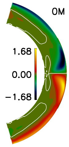
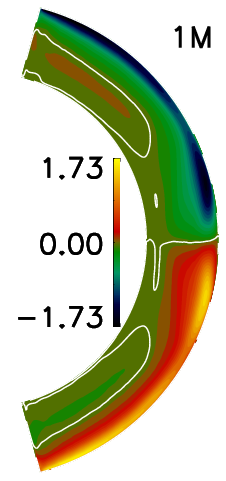
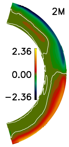
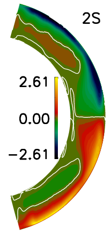
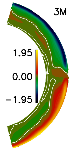
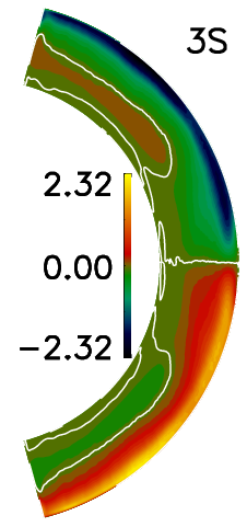
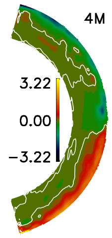
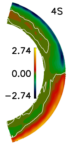
Figure 17: Time-averaged kinetic helicity $H_{\rm kin}=\overline{\mbox{\boldmath$\omega$}{}^{\prime}\cdot\mbox{\boldmath$u$}{}^{\prime}}$ in units of $10^{-3}$m$/$s² for M and S runs. White contours indicate zero values. We smooth the data over 100 neighboring points for runs A4M, A4S to make the data less noisy.

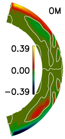
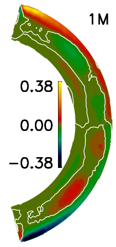
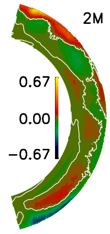
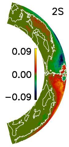
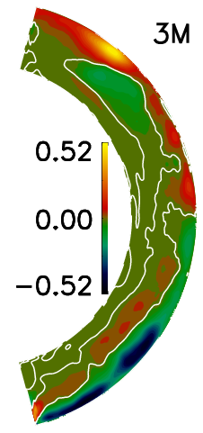
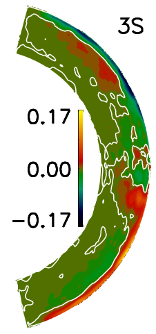
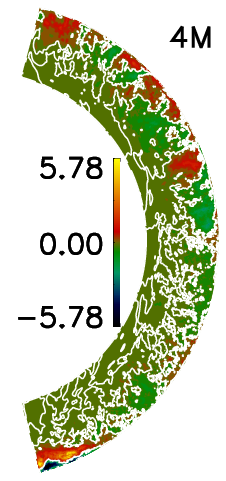
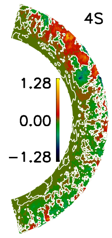
Figure 18: Time-averaged current helicity $H_{\rm cur}=\overline{\mbox{\boldmath$J$}{}^{\prime}\cdot\mbox{\boldmath$B$}{}^{\prime}}/\overline{\rho}$ in units of $10^{-3}$m$/$s² for M and S runs. White contours indicate zero values. We smooth the data over 40 and 100 neighboring points for runs 3M, 3S and 4M, 4S, respectively to make the data less noisy.

3.7 Kinetic and current helicities

One of the most important turbulent dynamo processes is the $\alpha$ effect (Steenbeck et al. 1966). Its strength can be estimated by the kinetic helicity density $H_{\rm kin}=\overline{\mbox{\boldmath$\omega$}{}^{\prime}\cdot\mbox{\boldmath$u$}{}^{\prime}}$, and the magnetic influence on it by the current helicity density $H_{\rm curr}=\overline{\mbox{\boldmath$J$}{}^{\prime}\cdot\mbox{\boldmath$B$}{}^{\prime}}/\overline{\rho}$ (e.g. Pouquet et al. 1976), here defined with an $1/\overline{\rho}$ factor:

$$\alpha\approx-H_{\rm kin}/3\tau_{\rm c}+H_{\rm curr}/3\tau_{\rm c},$$ (29)

where $\tau_{\rm c}$ is the turbulent correlation time, which in general does not need to be the same for the first and second term. In this work, we only look at these proxies (Figs. 17 and 18) and leave the detailed analysis of the $\alpha$ tensor and other turbulent transport coefficients to a future study.

As usual in rotating convection simulations, $H_{\rm kin}$ is predominantly negative in the upper half of the convection zone and positive below in the northern hemisphere while having the same pattern but opposite sign in the southern hemisphere, see Fig. 17. We find that the profile of $H_{\rm kin}$ is not much influenced by the increase of Re nor showing a large difference between S and M runs. We only find that the peak values of $H_{\rm kin}$ show a tendency to increase with increasing Re and that in Run 0M the maxima near the equator extend further into the convection zone.

The current helicity $H_{\rm curr}$ exhibits a different behavior. Similar to earlier results (e.g., Warnecke & Käpylä 2020), it is positive near the surface in the northern hemisphere, negative in the bulk, and positive again near the bottom of the domain for most of the M runs while having an analogous profile but with the opposite sign in the southern hemisphere. Increasing Re leaves the profile mostly unchanged but leads to an increase in the peak values, at least when comparing 0M and 1M with 2M and 3M.

Interestingly, the current helicity $H_{\rm curr}$, see Fig. 18, from the pure SSD runs follows the pattern of $H_{\rm kin}$ rather than that of $H_{\rm curr}$ of the corresponding M runs. The fact that the sign of $H_{\rm curr}$ is opposite in the cases with and without LSD is in line with the results of Warnecke et al. (2012), where the authors explain this sign change from simulations (Warnecke et al. 2011) and observations (Brandenburg et al. 2011) by a simple model. It suggests a sign change in $H_{\rm curr}$ to be expected when an LSD is absent compared to when it is present.

$H_{\rm curr}$ generated by the SSD is clearly smaller than the one generated by an LSD. Furthermore, $|H_{\rm curr}|$ is always (except for 4M) smaller than $|H_{\rm kin}|$ and therefore should not influence the $\alpha$ effect much, following Equation (29). However, the work by Warnecke & Käpylä (2020) shows that this approximation does not hold when comparing with $\alpha$ determined by the test-field method in cases where the magnitudes of $H_{\rm curr}$ and $H_{\rm kin}$ become comparable.

4 Conclusions

We have conducted global convective dynamo simulations of solar-like stars, wherein we varied viscosity, magnetic diffusivity, and SGS heat diffusivity to examine how the solutions depend on the fluid and magnetic Reynolds numbers. This enabled us to investigate the interaction between SSD and LSD and their effects on the overall dynamics. As a novel approach, we additionally investigated SSD in LSD-capable systems in isolation by suppressing the large-scale magnetic field.

As an outcome of these simulations, we have identified the following results: Magnetic runs with $\mbox{\rm Re}_{\rm M}\geq 140$ can excite an SSD, with its magnetic energy becoming comparable to that of the LSD at $\mbox{\rm Re}_{\rm M}\approx 550$. The total magnetic field energy appears to reach a maximum at $\mbox{\rm Re}_{\rm M}=120$ and decreases for runs with higher $\mbox{\rm Re}_{\rm M}$. Although the SSD becomes stronger at higher $\mbox{\rm Re}_{\rm M}$, the energy in the fluctuating field mildly decreases. As the mean field decreases by more than half compared to Runs 2M and 3M, the total magnetic energy is significantly weaker.

The scale of large-scale convective cells, also known as Banana cells, does not depend on the Reynolds numbers or the presence of LSD and SSD. The depth of the sub-adiabatic layers is mostly independent of Re, except at mid-latitudes. However, the Deardorff layer becomes thinner, allowing for a thicker overshoot and radiative zone for higher Re. The turbulent velocity $u^{\prime}_{\rm rms}$ increases with Re until $\mbox{\rm Re}=120$, after which it slightly decreases, even in the H runs. This indicates that the decrease at high Re is not due to the presence of SSD or LSD as found by HK21 and HKS22. The magnetic field in our simulations does not reach strong super-equipartition w.r.t. turbulent kinetic energy. Additionally, at small scales, the magnetic field is mostly at subequipartition. Furthermore, the energy in the large convective scales mildly decreases with Re, but this occurs in the H runs as well, suggesting that it cannot be attributed to the effects of SSD or LSD.

Differential rotation is strongly quenched in M runs with high Re, primarily due to the magnetic field of LSD rather than of SSD. The magnetic field affects the angular momentum distribution via the suppression of the Reynolds stresses and the emergence of strong Maxwell stresses.

The evolution of large-scale fields shows only a weak dependence on $\mbox{\rm Re}_{\rm M}$, with the equatorward migrating field mode disappearing for $\mbox{\rm Re}_{\rm M}\geq 60$ due to weaker shear at mid-latitudes. The irregular low-frequency mode at the bottom of the domain persists, and even the high-frequency mode near the surface is present in all relevant M runs. SSD is strongest in areas where the enthalpy flux is maximal, typically near the equator, where turbulent energy reaches its peak. The profiles of kinetic and current helicity do not vary much with $\mbox{\rm Re}_{\rm M}$, but there is a tendency for a mild increase in their peak values with $\mbox{\rm Re}_{\rm M}$. Interestingly, current helicity generated by pure SSD has the opposite sign to that of LSD. Our work shows that it is important to study the SSD-LSD interaction to fully understand the dynamics in the Sun and other stars.

Appendix A Diffusivity profiles

To avoid numerical artefacts near the latitudinal boundaries, we apply a profile for the diffusivities $\nu$ and $\eta$, increasing towards these boundaries. The profiles’ shape is shown in Fig. 19, it is determined by its width $\Delta\theta_{\nu}$ and $\Delta\theta_{\eta}$, respectively, and the ratio between the boundary value and the value at the equator,

$$\Delta_{\nu\eta}\equiv{\nu\,(\theta=\Theta_{0},\pi-\Theta_{0})\over\nu\,(\theta=\pi/2)}={\eta\,(\theta=\Theta_{0},\pi-\Theta_{0})\over\eta\,(\theta=\pi/2)}.$$ (30)

We choose the minimal possible values for $\Delta\theta_{\nu}$, $\Delta\theta_{\eta}$, and $\Delta_{\nu\eta}$, which keep the runs stable. It turns out that these adjustments are needed for runs with $\mbox{\rm Re}\geq 61$, see Table LABEL:runs for details.

Furthermore, for high resolution simulations ($\mbox{\rm Re}\geq 260$), the runs have a tendency to produce vortex-like structures at high latitudes. They are as such an interesting phenomenon (Käpylä et al. 2011b; Mantere et al. 2011), but they decrease the time step significantly. Hence, we decided to suppress them in this work by choosing $\Delta\theta_{\nu}=17^{\circ}$ and postpone their detailed study to the future.

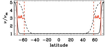
Figure 19: Latitudinal diffusivity profiles. Here shown for the viscosity $\nu$ with width $\Delta\theta_{\nu}=5^{\circ}$ (solid line) and $17^{\circ}$ (dashed), also directly indicated by vertical red lines. $\nu_{\rm m}$ is the equatorial value of $\nu$.

Appendix B Slope-limited diffusion

Figure 20: Visualisation of Equation (39): $Q$ as function of the slope ratio $\cal{R}$ for various $h_{\rm sld}$ (colored lines) with $n_{\rm sld}$=1 (solid) and $n_{\rm sld}$=2 (dashed).

Besides the constant diffusivity $\nu$, the H runs need additional explicit numerical diffusion to be stable. Our choice of using an enhanced luminosity at the bottom boundary, (see Käpylä et al. 2013, for details), causes the local Mach number $\mbox{\rm Ma}=|\mbox{\boldmath$u$}{}|/c_{\rm s}$ to increase near the surface to unusally high values. In the H runs, this can lead to numerical instabilities. The M and S runs are stable enough due to the presence of the magnetic field and do not need any additional diffusion. To let the numerical diffusion act only in regions, where it is needed, we employ slope-limited diffusion (SLD), newly implemented to the Pencil Code. It turns out that with our choice of parameters as specified below, we are able to stabilize the runs without influencing the overall dynamics much. In the following we will briefly describe implementation and parameter choice. Thereby we follow roughly Rempel et al. (2009) and Rempel (2014).

The main idea is to define the diffusive fluxes $f$ based on a slope limiter. At the cell interface $k+1/2$, they are given by

$$f_{k+1/2}=-{\textstyle{1\over 2}}c^{\rm sld}_{k+1/2}\,Q_{k+1/2}\,(u^{\rm R}_{k+1/2}-u^{\rm L}_{k+1/2}),$$ (31)

where $c^{\rm sld}$ is the characteristic speed, defined below. $u^{R}_{k+1/2}$ and $u^{L}_{k+1/2}$ are the right and left values at the cell interface of one of the velocity components. The subscript $k$ indicates the cell or grid-point in one particular coordinate direction. $u^{\rm R}$ and $u^{\rm L}$ are defined via

$$u^{\rm L}_{k-1/2} = u_{k-1}+\Delta u_{k-1}$$ (32)

$$u^{\rm R}_{k-1/2} = u_{k}-\Delta u_{k}$$ (33)

$$u^{\rm L}_{k+1/2} = u_{k}+\Delta u_{k}$$ (34)

$$u^{\rm R}_{k+1/2} = u_{k+1}-\Delta u_{k+1}$$ (35)

with the estimated slopes

$$\Delta u_{k}=\text{minmod}\,(u_{k}-u_{k-1},u_{k+1}-u_{k}),$$ (36)

where the minmod function is defined as

$$\text{minmod}\,(a,b)={\textstyle{1\over 2}}{\rm sgn}\,{}(a)\max\left[0,\min\left(|a|,{\rm sgn}\,{}(a)\,b\right)\right],$$ (37)

meaning

$$\text{minmod}\,\big{(}a,b\big{)}=\left.\begin{cases}\>+{\textstyle{1\over 2}}\min\big{(}|a|,|b|\big{)}\\ \>\phantom{+}0\\ \>\phantom{+}0\\ \>-{\textstyle{1\over 2}}\min\big{(}|a|,|b|\big{)}\end{cases}\right\}\>\text{for}\;\begin{cases}\>a>0,\,b>0\\ \>a<0,\,b>0\\ \>a>0,\,b<0\\ \>a<0,\,b<0\end{cases}.$$ (38)

The diffusive flux is additionally adjusted by

$$Q_{k+1/2}=\left[\min(1,h_{\rm sld}\,{\cal R}_{k+1/2})\right]^{n_{\rm sld}},$$ (39)

which controls the non-linearity and has values between 0 and 1. The parameter $h_{\rm sld}$ sets the strength of the diffusion for a given slope. If $h_{\rm sld}$=$\infty$, i.e. $Q=1$ Equation (31) represent a linear 2-order Lax-Friedrichs-scheme. The lower $h_{\rm sld}$, the less diffusive the scheme is. The non-linear factor $n_{\rm sld}$ can reduce the diffusion even further for small slopes. The slope ratio ${\cal R}$ is defined as

$${\cal R}_{k+1/2}={|u^{R}_{k+1/2}-u^{L}_{k+1/2}|\over|u_{k+1}-u_{k}|}.$$ (40)

Equation 39 implies that in regions where ${\cal R}_{k+1/2}\geq 1/h_{\rm sld}$, the diffusive flux is maximal and for regions, where ${\cal R}_{k+1/2}<1/h_{\rm sld}$ the diffusive flux is reduced, see Fig. 20 for an illustration. In this work, we use $h_{\rm sld}=2$ and $n_{\rm sld}=1$ for the density and $h_{\rm sld}=1$ and $n_{\rm sld}=2$ for all velocity components. The slope ratio ${\cal R}$ relates the differences at the cell interface to the difference of the cell centres, therefore indicated the relative slope strength. We note here that in Rempel et al. (2009) a similar scheme is used, which corresponds to $h_{\rm sld}=1$ and $n_{\rm sld}=2$. In the work of Rempel (2014), a different expression for $Q({\cal R})$ is used – see their Eq. (10), employing only one parameter instead of two. Detailed tests indicate no significant differences between his and our scheme.

The characteristic speed is derived from the signal (advection and wave) speeds in the system:

$$c^{\rm sld}=w^{\rm sld}_{\rm hyd}|\mbox{\boldmath$u$}{}|+w^{\rm sld}_{\rm ene}c_{\rm s}+w^{\rm sld}_{\rm mag}v_{\rm A},$$ (41)

where $v_{\rm A}$ is the Alfven speed, and the weights $w^{\rm sld}_{\ast}$ can be chosen depending on the nature of the problem. In this work, we set $w^{\rm sld}_{\rm hyd}=1$. and $w^{\rm sld}_{\rm ene}=0.001$; there is no magnetic contribution because we use SLD only for purely hydrodynamic runs. With these intercell values are calculated as a 1D linear interpolation.

$$c^{\rm sld}_{k+1/2}={c^{\rm sld}_{k}+c^{\rm sld}_{k+1}\over 2}.$$ (42)

Connecting the strength of the SLD term to the advection speeds via $c^{\rm sld}$ makes an extra time step constraint unnecessary.

The calculation of the diffusive fluxes is now performed at each grid point for all three directions seperately. With these three fluxes we can form a diffusive flux vector ${\mbox{\boldmath$f$}{}}_{\rm sld}=(f_{j})$, where $j$ indicates the coordinate direction. If the diffusive fluxes are calculated from a vector quantity, then each vector component builds its own flux vector and these together a diffusive flux tensor $\mbox{\boldmath${\cal F}$}{}_{\rm sld}$.

Now the diffusive fluxes are added to the momentum and continuum equations via

$${{\rm D}{}\mbox{\boldmath$u$}{}\over{\rm D}{}t}=...-\mbox{\boldmath$\nabla$}{}^{2\rm nd}\cdot\mbox{\boldmath${\cal F}$}{}^{u}_{\rm sld},\quad\quad{{\rm D}{}\ln\rho\over{\rm D}{}t}=...-\mbox{\boldmath$\nabla$}{}^{2\rm nd}\cdot{\mbox{\boldmath$f$}{}}^{\rho}_{\rm sld},$$ (43)

where $\mbox{\boldmath${\cal F}$}{}^{u}_{\rm sld}$ is the SLD tensor for the velocity and ${\mbox{\boldmath$f$}{}}^{\rho}_{\rm sld}$ is the SLD vector for the density. For simplicity, we use 2nd order finite differences for the divergence ($\mbox{\boldmath$\nabla$}{}^{2\rm nd}$). For the velocity we calculate the divergence for each component separately and show here the derivation for one velocity component only as an example in Cartesian coordinates. This can be analogously used also for the density.

$$\mbox{\boldmath$\nabla$}{}^{2\rm nd}\cdot{\mbox{\boldmath$f$}{}}^{u}_{\rm sld}=\sum_{j}\,\partial^{2\rm nd}_{j}\,f_{j}=\sum_{j}{f_{j}(jk_{+})-{f_{j}(jk_{-})}\over{j(jk_{+})-j(jk_{-})}}\\$$ (44)

where as above $j$ is the coordinate i.e. $x$, $y$, $z$ in the Cartesian case, $jk$ denotes the grid point under consideration in the direction of the coordinate $j$ and $jk_{+}$ and $jk_{-}$ is short for $jk+1/2$ and $jk-1/2$, respectively. This means the flux in the direction $j$ will be differentiated in the $j$ direction.

For spherical coordinates the Equation (44) is modified and reads for an SLD vector such as $\mbox{\boldmath$f$}{}^{\rho}_{\rm sld}$

$$\mbox{\boldmath$\nabla$}{}^{2\rm nd}\cdot\mbox{\boldmath$f$}{}_{\rm sld}=\sum_{\rm j}\partial^{2\rm nd}_{j}\,f_{j}$$ (45)

$$= {r^{2}(xk_{+})f_{x}(xk_{+})-r^{2}(xk_{-})f_{x}(xk_{-})}\over{r^{2}(xk)[r(xk_{+})-r(xk_{-})]}$$

$$+ {\sin(\theta(yk_{+}))f_{y}(yk_{+})-\sin(\theta(yk_{-}))f_{y}(yk_{-})}\over{r(xk)\sin(\theta(yk))[\theta(yk_{+})-\theta(yk_{-})]}$$

$$+ {f_{z}(zk_{+})-f_{z}(zk_{-})}\over{r(xk)\sin(\theta(yk))[\phi(zk_{+})-\phi(zk_{-})]},$$

for an SLD tensor such as ${\mbox{\boldmath${\cal F}$}{}}^{u}_{\rm sld}$

$$[\mbox{\boldmath$\nabla$}{}^{2\rm nd}\cdot\mbox{\boldmath${\cal F}$}{}_{\rm sld}]_{r} = {r^{2}(xk_{+})f^{r}_{x}(xk_{+})-r^{2}(xk_{-})f^{r}_{x}(xk_{-})}\over{r^{2}(xk)[r(xk_{+})-r(xk_{-})]}$$ (46)

$$+ {\sin(\theta(yk_{+}))f^{r}_{y}(yk_{+})-\sin(\theta(yk_{-}))f^{r}_{y}(yk_{-})}\over{r(xk)\sin(\theta(yk))[\theta(yk_{+})-\theta(yk_{-})]}$$

$$+ {f^{r}_{z}(zk_{+})-f^{r}_{z}(zk_{-})}\over{r(xk)\sin(\theta(yk))[\phi(zk_{+})-\phi(zk_{-})]}$$

$$- {f^{\theta}_{y}(yk_{+})+f^{\theta}_{y}(yk_{-})}\over{2r_{x(k)}}$$

$$- {f^{\phi}_{z}(zk_{+})+f^{\phi}_{z}(zk_{-})\over 2r_{x(k)}}$$

$$[\mbox{\boldmath$\nabla$}{}^{2\rm nd}\cdot\mbox{\boldmath${\cal F}$}{}_{\rm sld}]_{\theta} = {r^{2}(xk_{+})f^{\theta}_{x}(xk_{+})-r^{2}(xk_{+})f^{\theta}_{x}(xk_{-})}\over{r^{2}(xk)[r(xk_{+})-r(xk_{-})]}$$ (47)

$$+ {\sin(\theta(yk_{+}))f^{\theta}_{y}(yk_{+})-\sin(\theta(yk_{-}))f^{\theta}_{y}(yk_{-})}\over{r(xk)\sin(\theta(yk))[\theta(yk_{+})-\theta(yk_{-})]}$$

$$+ {f^{\theta}_{z}(zk_{+})-f^{\theta}_{z}(zk_{-})}\over{r(xk)\sin(\theta(yk))[\phi(zk_{+})-\phi(zk_{-})]}$$

$$- {f^{r}_{y}(yk_{+})+f^{r}_{y}(yk_{-})}\over{2r(xk)}$$

$$- {\cot{\theta(yk)}[f^{\phi}_{z}(zk_{+})+f^{\phi}_{z}(zk_{-})]}\over{2r(xk)}$$

$$[\mbox{\boldmath$\nabla$}{}^{2\rm nd}\cdot\mbox{\boldmath${\cal F}$}{}_{\rm sld}]_{\phi} = {r^{2}(xk_{+})f^{\phi}_{x}(xk_{+})-r^{2}(xk_{+})f^{\phi}_{x}(xk_{-})}\over{r^{2}(xk)[r(xk_{-})-r(xk_{-})]}$$ (48)

$$+ {\sin(\theta(yk_{+}))f^{\phi}_{y}(yk_{+})-\sin(\theta(yk_{-}))f^{\phi}_{y}(yk_{-})}\over{r(xk)\sin(\theta(yk))[\theta(yk_{+})-\theta(yk_{-})]}$$

$$+ {f^{\phi}_{z}(zk_{+})-f^{\phi}_{z}(zk_{-})}\over{r(xk)\sin(\theta(yk))[\phi(zk_{+})-\phi(zk_{-})]}$$

$$- {f^{r}_{z}(zk_{+})+f^{r}_{z}(zk_{-})}\over{2r(xk)}$$

$$- {\cot{\theta(y(k))}[f^{\theta}_{z}(zk_{+})+f^{\theta}_{z}(zk_{-})]}\over{2r(xk)},$$

where the superscripts of $f$ indicate coordinat of the quantity the diffusive flux is calculated of, e.g. $r$ for $u_{r}$.

The viscous heat due to the SLD ${\cal H}^{\rm sld}$ is defined at grid point $k$ as

$${\cal H}^{\rm sld}_{k}={\textstyle{1\over 2}}\sum_{i,j} \left\{\hskip 11.38109ptf^{u^{i}}_{j}(jk_{-}){\rho(jk)u^{i}(jk)-\rho(jk-1)u^{i}(jk-1)\over j(jk)-j(jk-1)}\right.$$

$$\hskip 5.69054pt+\left.f^{u^{i}}_{j}(jk_{+}){\rho(jk+1)u^{i}(jk+1)-\rho(jk)u^{i}(jk)\over j(jk+1)-j(jk)}\>\right\},$$ (49)

where $i$ is the component of $u$ and $j$ the coordinate direction. In spherical coordinates, this expression will be modified taken into account the appropriate derivatives. We note here that the heating expression implementation in MURAM (Rempel et al. 2009; Rempel 2014), only takes into account the derivative of the velocity and not the momentum, i.e. it neglects the changes in the density.

Using a mass diffusion introduces an additional mass flux, for which we compensated in the momentum and energy equations.

Appendix C Spectra of banana cells

To investigate how the scales of the banana cells depend on the Reynolds numbers, we calculate the power spectra of the kinetic energy density of the radial flow, ${E}^{r}_{\rm kin}$, near the surface ($r=r_{s}\equiv 0.98\,R$). For this, we cut out a thin latitudinal band around the equator ($\pm\,7.5\hbox{${}^{\circ}$}$) and calculate the power spectrum of ${E}^{r}_{\rm kin}$, averaged over latitude and time, as a function of the angular order $m$ for each run. We rely on the definition

$$\sum_{m}\widetilde{E}^{r}_{\rm kin}(m)=\sum_{m}\left\langle{{\textstyle{1\over 2}}\left|\,{\rm FFT}\left[\big{(}u_{r}\!\sqrt{\rho}\big{)}(r_{s})\right]\!(m)\right|^{2}}\right\rangle_{\theta t}={r_{s}\over 2}\left\langle{\left(u_{r}^{2}\rho\right)(r_{s})}\right\rangle_{\theta\phi t},$$ (50)

where the tilde and the operator ${\rm FFT}$ indicate the Fourier transform. The spectra are shown in Fig. 21 for all runs, including the Re dependence of the $m$ of their maxima. Only a weak Re dependence is visible. The spectra of the M runs, except M0, peak around $m=40$, whereas those of the H runs peak at slightly lower $m\approx 32$. The S run spectra peak at $m=32$ for moderate $\mbox{\rm Re}_{\rm M}$ and at $m=40$ for high $\mbox{\rm Re}_{\rm M}$.

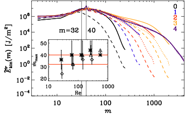
Figure 21: Longitudinal power spectra of the radial kinetic energy density, $\widetilde{E}^{r}_{\rm kin}$, near the surface $r$=0.98$\,R$ for a narrow latitudinal band around the equator ($\pm\,7.5\hbox{${}^{\circ}$}$). The colors indicate the run sets and the line style/symbols the run type: solid/asterisk (M), dashed/diamonds (H) and dotted/triangles (S). The spectra are averaged over the $\theta$ bands and time. The inlay shows the $m$ value of the maxima as a function of Re for all runs. The errors are calculated using an 80% range around the peak. The values $m=32$ and $m=40$ are indicated by black vertical and (in inlay) red horizontal lines, respectively.