Separation Power of Equivariant Neural Networks

Abstract

The separation power of a machine learning model refers to its capacity to distinguish distinct inputs, and it is often employed as a proxy for its expressivity. In this paper, we propose a theoretical framework to investigate the separation power of equivariant neural networks with point-wise activations. Using the proposed framework, we can derive an explicit description of inputs indistinguishable by a family of neural networks with given architecture, demonstrating that it remains unaffected by the choice of non-polynomial activation function employed. We are able to understand the role played by activation functions in separability. Indeed, we show that all non-polynomial activations, such as ReLU and sigmoid, are equivalent in terms of expressivity, and that they reach maximum discrimination capacity. We demonstrate how assessing the separation power of an equivariant neural network can be simplified to evaluating the separation power of minimal representations. We conclude by illustrating how these minimal components form a hierarchy in separation power.

1 Introduction

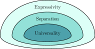
Figure 1: Expressive power of neural networks assess their ability to solve complex tasks. Although universality is traditionally investigated to quantify expressivity, invariant and equivariant models first need to be understood in terms of their separation power.

Alongside the proliferation and success of equivariant models [1, 2, 3], there has been a growing interest in understanding the fundamental reasons behind their performances, and in assessing their expressive power [4, 5]. For traditional deep learning approaches, this expressive power is usually quantified in terms of universality [6], or their ability to approximate any element of a given class of functions to arbitrary precision. However, universality is not directly applicable to neural networks that incorporates invariances of the data [7], since they necessarily act by identifying pairs of inputs that are equivalent under the given set of transformations. This feature creates a complex interaction between the network’s ability to discriminate different input data, and the invariant or equivariant structure that they are trying to preserve. Assessing expressivity thus requires first a fine-grained analysis of a network’s separation power – the capacity of a model to distinguish distinct inputs, which is a necessary condition for the universality of the models [8]. In the graph learning community, which is a paramount domain where invariant and equivariant models are studied [3, 9, 10], networks are required to be invariant or equivariant under the group of permutations of the graph’s nodes. In this domain the primary methods for comparing separation power are the Weisfeiler-Leman (WL) isomorphism test [11] and homomorphism counting [12]. Significant attention has been devoted to studying this property for graph processing models such as Graph Neural Networks (GNNs) [13, 14, 15], Invariant Graph Networks (IGNs) [3, 16], and subgraph GNNs [17, 10]. However, the WL test and homomorphism counting, along with their variants, have severe limitations imposed by their combinatorial nature. In particular, recent research [8] have highlighted the necessity of developing expressivity measures applicable to models that process data beyond relational structures, such as geometric graphs. In this paper we contribute to this effort by studying the separation power of a more general class of equivariant neural networks, which are not covered by the existing results but are of significant practical interest. Namely, we focus on the family of neural networks with regular convolutions [18], i.e., networks with non-polynomial point-wise activations, finite-dimensional representations, and equivariance with respect to the action of finite groups acting on representations as permutations. This class is rich enough to comprise many models of common interest, such as IGNs [3], Convolutional Neural Networks (CNNs) [19], and Icosahedral CNNs [20]. We are able to precisely describe the set of input pairs identified by neural networks with a fixed architecture, in contrast to other approaches that only provide upper bounds on the expressiveness of IGNs [21] or lower bounds that imply arbitrary network width for the features [4]. To study the separation power of the entire class of equivariant networks with fixed architecture, we consider the dual problem of characterizing the set of points that are identified by the networks. By constructing a suitable twin network, we show that the set of identified points corresponds to the set of common zeros of a modified set of networks (Section 5.1). We then describe this set in an exhaustive way by introducing an explicit formula which, remarkably, is recursive over the networks depth (Section 5.2). This explicit result has a number of relevant consequences on the design of equivariant neural network architectures, which are determined by their activation function, their width, and the blocks of different type and multiplicity that form their affine equivariant layers. Namely, we show that any non-polynomial activation yields exactly the same separation power. Furthermore, we prove that the multiplicity of the blocks in the affine layers does not affect the separation power of the networks (Section 5.3), and we demonstrate that the separation power of different block types forms a hierarchy, corresponding to the partial ordering of sub-groups of the symmetry group with respect to which the model is equivariant (Section 5.4). This result is in analogy with the hierarchy of the WL tests for graph learning tasks.

In summary, our contributions can be summarized as follows:

• We address the separation power of equivariant neural networks by fully characterizing, with a formula which is recursive over the network depth, the set of points which are identified by networks of fixed architecture.

• We show that any non-polynomial activation is equivalent in terms of separation power, and that they reach the maximum separability capacity of the family of neural networks induced by a fixed architecture.

• We demonstrate how the block decomposition of layers impacts separability and illustrate how these minimal components form a hierarchy in separation power.

2 Related Work

Recently, equivariant deep learning models have gained popularity [22, 18, 23], being successful in diverse fields such as computer graphics [24], galaxy morphology prediction [25], computational biology [26], and computational chemistry [27]. In the case of permutation equivariance, the WL test has been adopted as the fundamental tool to measure the expressivity of GNNs [28, 29] and has been used to derive upper bounds [30] and lower bounds [4] on the expressiveness of IGNs and GNNs [31]. Recently, homomorphism counting has been proposed as a more fine-grained measure of expressivity for GNNs [32], capable of assessing the separation power of subgraph GNNs and their variants [17, 33, 10]. In [8], the authors address the problem of separability by generalizing the WL test from combinatorial structures to geometric graphs. Other works that are related to the study of neural network separability include specific universality results for equivariant networks [34, 5, 35, 36, 37, 38]. In fact, it has been demonstrated in [28] that a universal model within the class of functions invariant with respect to certain symmetries is also maximally separating, modulo symmetries.

3 Preliminaries

3.1 Groups and Equivariance

We aim to define functions that are symmetric with respect to specific transformations. Groups, which are particularly useful for computation and technical manipulation, consist of transformations that fulfill certain criteria: the elements can be combined, each element has an inverse, and there is a neutral element with respect to composition. While group theory efficiently studies symmetries and transformations from a purely algebraic perspective, it needs to be adapted to the linear algebra framework required for defining neural networks. Representation theory acts as a dictionary for translating between these two languages, showing how abstract groups can be mapped to sets of matrices that themselves form groups. For an overview, see [39]. Let $X$ be a finite set and $G$ a finite group acting on it. A permutation representation of $G$ is an action of $G$ on $\operatorname{\mathbb{R}}^{X}$ such that $g(e_{x})=e_{gx}$ for each $g\in G$ and $x\in X$. Let $\operatorname{\mathbb{R}}^{X}$ and $\operatorname{\mathbb{R}}^{Y}$ be permutation $G$-representations, we say that a function $\phi:\operatorname{\mathbb{R}}^{X}\to\operatorname{\mathbb{R}}^{Y}$ is $G$-equivariant if $\phi(gv)=g\phi(v)$ for each $v\in\operatorname{\mathbb{R}}^{X}$ and $g\in G$. We denote by $\operatorname{Hom}(\mathbb{R}^{X},\mathbb{R}^{Y})$ the set of linear maps between $\mathbb{R}^{X}$ and $\mathbb{R}^{Y}$, and by $\operatorname{Hom}_{G}(\mathbb{R}^{X},\mathbb{R}^{Y})$ the subset of $G$-equivariant linear maps. Similarly, we refer to the set of affine maps between $\mathbb{R}^{X}$ and $\mathbb{R}^{Y}$ as $\operatorname{Aff}(\mathbb{R}^{X},\mathbb{R}^{Y})$, and the set of $G$-equivariant affine maps as $\operatorname{Aff}_{G}(\mathbb{R}^{X},\mathbb{R}^{Y})$. Note that $\operatorname{Hom}(\mathbb{R}^{X},\mathbb{R}^{Y})$, $\operatorname{Aff}(\mathbb{R}^{X},\mathbb{R}^{Y})$, and their equivariant counterparts are real vector spaces with respect to addition and scalar multiplication. Moreover, [40] shows that each affine map $\phi:\mathbb{R}^{X}\to\mathbb{R}^{Y}$ has a unique decomposition $\phi=\tau_{v}\circ\phi^{\prime}$, where $\phi^{\prime}$ is a linear map and $\tau_{v}$ is a translation by a vector $v\in\mathbb{R}^{Y}$, and furthermore, that an affine map $\phi=\tau_{v}\circ\phi^{\prime}$ is equivariant if and only if its linear part $\phi^{\prime}$ is equivariant and $v$ is invariant with respect to the action of $G$. We have relevant linear morphisms $\lambda:\operatorname{Aff}_{G}(V,W)\to\operatorname{Hom}_{G}(V,W)$, which projects an affine map onto its linear part, and $\tau:\operatorname{Aff}_{G}(V,W)\to W^{G}$, which projects an affine map onto its translational part. Thanks to the unique decomposition of affine maps, each subspace $M<\operatorname{Aff}(\mathbb{R}^{X},\mathbb{R}^{Y})$ is characterized by the subspaces $\lambda(M)$ and $\tau(M)$. Indeed, it can be reconstructed using the isomorphism $\lambda(M)\times\tau(M)\to M$, defined by $(\phi^{\prime},v)\mapsto\tau_{v}\phi^{\prime}$. Both components are finitely generated, so $M$ is associated by the set $\{\phi^{\prime}_{i},\tau_{v_{j}}\}_{i,j}$, where $\{\phi^{\prime 1},\dots,\phi^{\prime h}\}$ is a finite set of linear maps that generate $\lambda(M)$ and $\{v_{1},\dots,v_{k}\}$ is a finite set of invariant vectors that generate $\tau(M)$.

3.2 Equivariant Neural Networks

With all the necessary definitions in place, we can now introduce the notion of equivariant neural network. Our study will focus on neural networks that are equivariant with respect to finite groups, have point-wise continuous activation functions, and whose hidden representations are permutation representations.

Definition 3.1.

Let $G$ be a finite group and $V,W$ be two $G$-representations which are respectively the input and output space. A $G$-equivariant neural network with point-wise activations is a composition

$$\eta:V\xrightarrow{\phi_{1}}\operatorname{\mathbb{R}}^{X_{1}}\xrightarrow{\tilde{\sigma}}\operatorname{\mathbb{R}}^{X_{1}}\xrightarrow{\phi_{2}}\operatorname{\mathbb{R}}^{X_{2}}\xrightarrow{\tilde{\sigma}}\cdots\xrightarrow{\phi_{d}}\operatorname{\mathbb{R}}^{X_{d}}\xrightarrow{\tilde{\sigma}}\operatorname{\mathbb{R}}^{X_{d}}\xrightarrow{\phi_{d+1}}W$$

where $X_{i}$ are finite sets with $G$ acting on them, $\phi_{i}\in\operatorname{Aff}_{G}(\operatorname{\mathbb{R}}^{X_{i-1}},\operatorname{\mathbb{R}}^{X_{i}})$ is an affine $G$-equivariant map, and $\tilde{\sigma}$ are point-wise activations induced by a continuous function $\sigma:\operatorname{\mathbb{R}}\rightarrow\operatorname{\mathbb{R}}$, defined as $\tilde{\sigma}(\sum_{x\in X_{i}}\alpha_{x}e_{x})=\sum_{\alpha\in X_{i}}\sigma(\alpha_{x})e_{x}$.

As shown in Figure 1, in machine learning practice, we are interested in specific function spaces that can approximate, learn, and train on the required task. In the following, we define the space of neural networks with a fixed architecture. This means that the input, output, and intermediate representations of the neural networks are fixed, as well as the activation function. However, the linear mappings between representations can vary within appropriate subspaces of affine mappings. This latter restriction is necessary for two reasons. The first reason is practical: to ensure our framework aligns as closely as possible with real-world practices, we must adapt it, considering that deep learning models are rarely trained on the entire family of equivariant networks but are instead restricted to specific cases. For example, in computer vision, convolutional filters are chosen to be of fixed and small size, representing only a limited subspace of the possible equivariant linearities available. The second reason is technical. This notational complexity will enable us to use the twin neural network trick, which is central to the proof of Theorem 1.

Definition 3.2.

Given subsets $M_{i}$ of $\operatorname{Aff}_{G}(\operatorname{\mathbb{R}}^{X_{i}},\operatorname{\mathbb{R}}^{X_{i+1}})$, we can define the space $\operatorname{\mathcal{N}}_{\sigma}(M_{1},\dots,M_{d})$ of equivariant networks with fixed architecture as the set of all equivariant neural networks with point-wise activations $\tilde{\sigma}$ induced by $\sigma$, and with affine parts constrained by the $M_{i}$s, i.e., $\phi_{i}\in M_{i}$ for each $i$. When $M_{i}=\operatorname{Aff}_{G}(\operatorname{\mathbb{R}}^{X_{i}},\operatorname{\mathbb{R}}^{X_{i+1}})$ are the entire sets of affine maps, we will simply write $\operatorname{\mathcal{N}}_{\sigma}(\operatorname{\mathbb{R}}^{X_{1}},\dots,\operatorname{\mathbb{R}}^{X_{d}})$.

In Definition 3.2, we specify no further structure on $M_{i}$ beyond it being a simple subset of $\operatorname{Aff}_{G}(\operatorname{\mathbb{R}}^{X_{i}},\operatorname{\mathbb{R}}^{X_{i+1}})$, even though we will mostly consider $M_{i}$ to be a linear subspace. This more general definition is due to technical reasons involving the proof of Theorem 1 and Lemma 4, but readers not interested in the technical details should just assume $M_{i}$ to be a linear subspace.

In this work we will study how architecture choice influences the separation power of the family of neural networks with such structure. In particular, we want to understand how the choices of $\sigma$, $\operatorname{\mathbb{R}}^{X_{i}}$, and $M_{i}$ affect $\rho(\operatorname{\mathcal{N}}_{\sigma}(M_{1},\dots,M_{d}))$ (see (1)).

4 The Relevance of Separability

The universality property of neural networks, or they ability to approximate any element of a given class of functions to arbitrary precision, has attracted significant attention in the machine learning community. To establish a systematic study of this property, one needs to understand which is the set of functions that can reasonably be approximated, and what are the architectures that are suitable for this task. In this paper we study the expressive power of equivariant neural networks by taking a step back from universality and focusing instead on their separation power. This concept is meaningful for general classes of functions, and we discuss in this section its significance and relation with the notion of universality (Figure 1).

We first give the following definition, where our interest will mainly be in sets $\operatorname{\mathcal{C}}\subseteq\operatorname{\mathcal{C}}(X,Y)$ of continuous functions between topological spaces $X$ and $Y$, since this includes the set of equivariant neural networks of interest (Section 3.2).

Definition 4.1.

For given sets $X,Y$, a function $f:X\rightarrow Y$ separates two points $\alpha,\beta\in X$ if $f(\alpha)\neq f(\beta)$. A family of functions $\operatorname{\mathcal{C}}$ from $X$ to $Y$ separates $\alpha,\beta\in X$ if there exist a function $f\in\operatorname{\mathcal{C}}$ separating $\alpha$ and $\beta$. If a function or a family of functions do not separate two points, we say that it identifies them.

By grouping together sets of points that are identified by $\operatorname{\mathcal{C}}$, we may define on $X$ an equivalence relation

$$\rho(\operatorname{\mathcal{C}})=\{(\alpha,\beta)\in X\times X\,|\,f(\alpha)=f(\alpha)\text{ for each }f\in\operatorname{\mathcal{C}}\}.$$ (1)

We address the problem of characterizing $\rho(\operatorname{\mathcal{C}})$ when $\operatorname{\mathcal{C}}$ is the set of all equivariant neural networks with a certain given architecture (Definition 3.1), and this offers significant advantages. First of all, this point of view is tailored to the practice: we provide results that hold for any network with a given structure, meaning that they remain valid under the optimization of the parameters of the network, and independently of the training dataset, the loss function, and the optimization method. Moreover, the study of the separation power for fixed architectures allows us to understand how this architecture can be improved: we discuss if and how common modifications of a fixed architecture, namely the width (Section 5.3) and structure of the intermediate layers (Section 5.4) lead to an improved separation power.

Finally, this characterization provides a framework that allows us to address questions along the two following directions:

Q1

Given a pair of points that need to be separated, which are the architectures $\operatorname{\mathcal{C}}$ that separates them, i.e., $\rho(\operatorname{\mathcal{C}})$ does not contain it?

Q2

Can we design sequences of networks with architectures of increasing separation power that can approximate continuous functions with separation power stronger than $\operatorname{\mathcal{C}}$?

Answering these questions will prove highly valuable to address universality, and in particular to understand how to design sequences of architectures that can approximate, in the limit, all functions from a given class.

5 Main Results

In this section, we lay the foundation for understanding the effect that architectural choices have on the separation power of a family of neural networks with a fixed architecture. We aim to demonstrate that non-polynomial activations achieve maximal separation power and to provide a recursive formula for explicitly computing points identified by this family of functions. This is the most technical result presented in this work and requires proper setup to be accurately stated. We will begin by describing and formulating the twin network trick in Section 5.1. This will be the main tool for transforming a separation problem into a zero locus problem, which we will solve in Section 5.2. We will conclude by stating and proving Corollary 1, which asserts that whenever the activations are chosen to be non-polynomial, they do not affect the separation power.

5.1 The Twin Network Trick

In this part of the paper, we explain the twin network trick, which allows us to transform a network separation problem into a zero locus problem for neural networks. This transformation enables us to solve the problem more easily using the recursive techniques explained in Section 5.2. Specifically, a zero locus problem involves computing all the points that are mapped to zero by all the neural networks in the chosen family.

More precisely, the identification equivalence relation (1) can be reformulated as the following zero locus problem: $(\alpha,\beta)\in\rho(\operatorname{\mathcal{N}}_{\sigma}(M_{1},\dots,M_{d}))$ if and only if

$$\eta(\alpha)-\eta(\beta)=0\;\;\forall\eta\in\operatorname{\mathcal{N}}_{\sigma}(M_{1},\dots,M_{d}).$$ (2)

The key idea is to observe that (2) actually reduces to a zero locus problem involving twin networks. As illustrated in Figure 2, the twin network $\overline{\eta}:V\oplus V\rightarrow W$, defined by

$$\overline{\eta}(\alpha,\beta)=\eta(\alpha)-\eta(\beta),$$ (3)

is itself a neural network with the same depth as $\eta$ but with a different architecture, namely $\overline{\eta}\in\operatorname{\mathcal{N}}_{\sigma}(\overline{M}_{1},\dots,\overline{M}_{d-1},M^{\prime}_{d})$ where $M^{\prime}_{d}=\{(x,y)\mapsto\phi(x)-\phi(y)\,|\,\phi\in M_{d}\}$, and

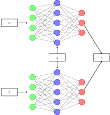
Figure 2: The twin network trick illustrated. Evaluating two copies of $\eta$ on $\alpha$ and $\beta$, and subtracting the resulting outputs, is equivalent to evaluating the twin network $\overline{\eta}$ on $(\alpha,\beta)$.

$$\overline{M}_{i}=\left\{\overline{\phi}=\begin{bmatrix}\phi&0\\ 0&\phi\end{bmatrix}\,\big{|}\,\phi\in M_{i}\right\}.$$

Thanks to the definition of the twin network, we can restate the identification problem in Equation 2 as the equivalent zero locus problem of finding all $\overline{\beta}$ in $V\oplus V$ that solve

$$\overline{\eta}(\overline{\beta})=0\;\forall\overline{\eta}\in\operatorname{\mathcal{N}}_{\sigma}(\overline{M}_{1},\dots,\overline{M}_{d-1},M^{\prime}_{d}).$$

In summary, all these observations can be synthesized into the following proposition, directly linking the identification relation to a zero locus.

Proposition 1.

For a family $\operatorname{\mathcal{F}}$ of continuous functions $\operatorname{\mathcal{C}}(X,V)$ between a topological space $X$ and a real vector space $V$, let

$$\operatorname{\mathcal{I}}(\operatorname{\mathcal{F}})=\{\beta\in X\,|\,\eta(\beta)=0\,\forall\eta\in\operatorname{\mathcal{F}}\}.$$

be the zero locus of $\operatorname{\mathcal{F}}$. Then we have

$$\rho(\operatorname{\mathcal{N}}_{\sigma}(M_{1},\dots,M_{d}))=\\ \operatorname{\mathcal{I}}(\operatorname{\mathcal{N}}_{\sigma}(\overline{M}_{1},\dots,\overline{M}_{d-1},M^{\prime}_{d})).$$

We are thus tasked with finding the set of common zeros for all elements in a new class of twin networks. To study this problem, particular attention must be paid to the bias term. In truth, the presence of bias in all the entries of the hidden representations is a necessary condition for our theory to work. Nevertheless, our assumptions regarding the bias term are always satisfied in standard practice. Without bias in all entries, the scenario becomes more complex, as we show in Section 6.2. The following definition formalizes this kind of bias and its opposite, where the bias is always zero.

Definition 5.1.

Let $M<\operatorname{Aff}_{G}(V,\operatorname{\mathbb{R}}^{X})$ be a linear subspace. We say that $M$ presents complete bias if there exists an element $y$ in its translational part $\tau(M)$ such that $y_{x}\neq 0$ for each $x\in X$; otherwise, we say that $M$ has incomplete bias. In particular, we say that $M$ has null bias if its translational part $\tau(M)$ is zero; in other words, $M<\operatorname{Hom}_{G}(V,\operatorname{\mathbb{R}}^{X})$.

Note that Equation 3 ensures that $\overline{M}_{i}$ has complete bias whenever $M_{i}$ does. Moreover, $M^{\prime}_{d}$ always has null bias, independently of the bias type of $M_{d}$. We have now presented all the tools needed to state and prove Theorem 1, which will be the main objective of the next section.

5.2 Main Theorem

In the previous sections, thanks to Proposition 1, we have translated the problem of computing the identification relation $\rho(\operatorname{\mathcal{N}}_{\sigma}(M_{1},\dots,M_{d}))$ into the problem of computing the zero locus $\operatorname{\mathcal{I}}(\operatorname{\mathcal{N}}_{\sigma}(\overline{M}_{1},\dots,\overline{M}_{d-1},M^{\prime}_{d}))$. This conversion is relevant, as the computation of the zero locus for a family of particular neural networks can be achieved using the recursive formula proposed by Theorem 1, which we will now state and prove.

Roughly speaking, the theorem shows that the set $\operatorname{\mathcal{I}}$ of a family of $d$-layers networks can be computed as suitable intersections and unions of sets $\operatorname{\mathcal{I}}$ corresponding to certain $(d-1)$-layers networks, thus recursively reducing the problem to incrementally shorter depths. Moreover, these shallower networks are obtained by reduction operations over the original ones: the last layer is removed, and the penultimate one is replaced by a suitable linearization.

Theorem 1.

Let $M_{1},\dots,M_{d-1}$ have complete bias and let $M_{d}$ have null bias. Denote as $\{\phi^{d+1,1},\dots,\phi^{d+1,s_{d}}\}$ a set of generators of $M_{d}$, and let $\operatorname{\mathcal{P}}_{n}$ be the set of all partitions of $[n]$. Define furthermore

$$\Psi_{h,k}=\{\operatorname{\mathcal{P}}\in\operatorname{\mathcal{P}}_{n}\,|\,\sum_{i\in P}\phi^{d+1,h}_{ki}=0,\,\forall P\in\operatorname{\mathcal{P}}\}.$$

If $\sigma$ is a non-polynomial activation function, then we have the following formula recursive with respect to network depth

$$\operatorname{\mathcal{I}}(\operatorname{\mathcal{N}}_{\sigma}(M_{1},\dots,M_{d}))=\bigcap_{h,k}\bigcup_{P\in\Psi_{h,k}}\bigcap_{i,j\in P}\operatorname{\mathcal{I}}(\operatorname{\mathcal{N}}_{\sigma}(M_{1},\dots,M_{d-2},(M_{d-1})_{ij})),$$ (4)

where $(M_{d-1})_{ij}=\{\phi^{\prime}:x\mapsto\pi_{i}\phi(x)-\pi_{j}\phi(x)\,|\,\phi\in\lambda(M_{d-1})\}$, $\pi_{i}:\operatorname{\mathbb{R}}^{X}\rightarrow\operatorname{\mathbb{R}}$ is the projection on the $i$-th component of $\operatorname{\mathbb{R}}^{X}$ for each $i$ in $X$, and $\lambda(M_{d-1})$ is linear part of $M_{d-1}$.

Proof.

Let $\operatorname{\mathcal{F}}_{i}=\{\phi^{i+1,1},\dots,\phi^{di+1,s_{i}}\}$ be a generating set for the linear part of $M_{i}$. By Lemma 3 we know that $\operatorname{\mathcal{I}}(\operatorname{\mathcal{N}}_{\sigma}(M_{1},\dots,M_{d}))=\operatorname{\mathcal{I}}(\operatorname{\mathcal{N}}_{\sigma}(M_{1},\dots,\operatorname{\mathcal{F}}_{d}))$. Hence $\beta$ belongs to $\operatorname{\mathcal{I}}(\operatorname{\mathcal{N}}_{\sigma}(M_{1},\dots,\operatorname{\mathcal{F}}_{d}))$ if and only if

$$\eta^{d,h}_{k}(\beta)=\sum_{i}\phi_{ki}^{d+1,h}\sigma\Big{(}\sum_{t}x_{t}\eta_{i}^{d-1,t}(\beta)+y_{i}\Big{)}=0$$ (5)

for each $h$ and $k$ where $\eta_{i}^{d-1,t}$ is a neural network in $\operatorname{\mathcal{N}}_{\sigma}(M_{1},\dots,M_{d-2},\operatorname{\mathcal{F}}_{d-1})$. Thanks to Theorem 4, if $\sigma$ is non-polynomial then $\beta$ solves the system $\sum_{i}\phi_{ki}^{d+1,h}\sigma\Big{(}\sum_{t}x_{t}\eta_{i}^{d-1,t}(\beta)+y_{i}\Big{)}=0$ if and only if $\eta_{i}^{d-1,t}(\beta)=\eta_{j}^{d-1,t}(\beta)$ for each $i,j\in P$ for each $P\in\operatorname{\mathcal{P}}$ for each partition $\operatorname{\mathcal{P}}$ of $[n]$ such that $\sum_{i\in P}\phi_{ki}^{d+1,h}=0$ for each $P\in\operatorname{\mathcal{P}}$. Note that $\beta$ solves the equation $\eta_{i}^{d-1,t}(\beta)-\eta_{j}^{d-1,t}(\beta)=0$ for each $t$ if and only if $\beta$ belongs to $\operatorname{\mathcal{N}}(M_{1},\dots,M_{d-2},(M_{d-1})_{ij})$. ∎

Remark 1.

Note that Theorem 1 and Corollary 1 could be stated with different activation functions for each layer, provided that all of them are non-polynomial. For readability and simplicity of notation, we have stated these results using a single activation function.

Although the actual execution of Formula 4 requires superpolynomial time, this recursive approach is particularly useful for deriving relevant properties of the identification relation, such as the influence of activations on separation power. The following corollary states that the choice of activation function is irrelevant in terms of separability, as long as activations are non-polynomial.

Corollary 1.

Let $\sigma$ and $\sigma^{\prime}$ be two continuous non-polynomial activations. Then

$$\operatorname{\mathcal{I}}(\operatorname{\mathcal{N}}_{\sigma}(M_{1},\dots,M_{d}))=\operatorname{\mathcal{I}}(\operatorname{\mathcal{N}}_{\sigma^{\prime}}(M_{1},\dots,M_{d})).$$

Proof.

We prove the equality by induction on $d$. Note that if $d=1$ then $\operatorname{\mathcal{I}}(\operatorname{\mathcal{N}}_{\sigma}(M_{1}))=\operatorname{\mathcal{I}}(M_{1})$ which does not depend on $\sigma$. Now suppose that $\operatorname{\mathcal{I}}(\operatorname{\mathcal{N}}_{\sigma}(M_{1},\dots,M_{d-1}))$ does not depends on $\sigma$ for each sequence $M_{1},\dots,M_{d-1}$. Then, observing Equation 4

$$\operatorname{\mathcal{I}}(\operatorname{\mathcal{N}}_{\sigma}(M_{1},\dots,M_{d}))=\bigcap_{h,k}\bigcup_{P\in\Psi_{h,k}}\bigcap_{i,j\in P}\operatorname{\mathcal{I}}(\operatorname{\mathcal{N}}_{\sigma}(M_{1},\dots,M_{d-2},(M_{d-1})_{ij})),$$

we note that $\operatorname{\mathcal{I}}(\operatorname{\mathcal{N}}_{\sigma}(M_{1},\dots,M_{d}))$ is independent of $\sigma$ as indices such as $h,k$ and $i,j$ are independent of $\sigma$, as well as $\operatorname{\mathcal{I}}(\operatorname{\mathcal{N}}_{\sigma}(M_{1},\dots,M_{d-2},(M_{d-1})_{ij}))$ is by inductive hypothesis. ∎

Remark 2.

Note that by the proof of Theorem 1 and Corollary 1, if $\sigma$ is a non-polynomial activation function and $\sigma^{\prime}$ is a polynomial activation function, then

$$\rho(\operatorname{\mathcal{N}}_{\sigma}(M_{1},\dots,M_{d}))\subseteq\rho(\operatorname{\mathcal{N}}_{\sigma^{\prime}}(M_{1},\dots,M_{d})).$$

Hence, non-polynomial activation functions have equivalent maximal separation power.

Remark 3.

Here, we demonstrate that the complete bias assumption is necessary for all non-polynomial activations to achieve maximal separation power. Specifically, let us examine the separation power of the set of shallow neural networks where all representation spaces are one-dimensional and the hidden layer has a null, and therefore incomplete, bias term. The main concern is the separability of opposite inputs $\beta$ and $-\beta$. This reduces to study the identification equation

$$y\sigma(\beta x)=y\sigma(-\beta x)$$

for each $x,y\in\operatorname{\mathbb{R}}$. Any even function $\sigma$, including non-polynomial ones, solves this equation but does not achieve maximal separation power, which could be reached by adding a bias term, as shown in Remark 2.

5.3 The Role of Intermediate Representations

In this section, we show that if a hidden representation $\operatorname{\mathbb{R}}^{X}$ can be decomposed as $\operatorname{\mathbb{R}}^{X^{\prime}}\oplus\operatorname{\mathbb{R}}^{X^{\prime\prime}}$, then the separation power of networks with the hidden representation $\operatorname{\mathbb{R}}^{X}$ can be easily reduced to the combined separation power of two distinct families of neural networks with hidden representations $\operatorname{\mathbb{R}}^{X^{\prime}}$ and $\operatorname{\mathbb{R}}^{X^{\prime\prime}}$. Indeed, Theorem 2 shows that the identification equivalence relation of the networks defined on $\operatorname{\mathbb{R}}^{X}$ is the intersection of the identification equivalence relations of the networks defined on $\operatorname{\mathbb{R}}^{X^{\prime}}$ and $\operatorname{\mathbb{R}}^{X^{\prime\prime}}$. This result is relevant because it implies that, given a decomposition of each hidden representation $\operatorname{\mathbb{R}}^{X}$ into a sum of minimal factors, we can reduce the study of the separation power of families of neural networks to the study of the separation power of families of neural networks defined on minimal representations. This will be the topic of Section 5.4.

For now, we focus on developing the notation necessary to state and prove Theorem 2. The structure of our network of interest is as follows:

$$\eta:V\xrightarrow{\phi_{1}}\operatorname{\mathbb{R}}^{X_{1}}\xrightarrow{\tilde{\sigma}}\cdots\xrightarrow{\phi_{i}}\operatorname{\mathbb{R}}^{X^{\prime}_{i}}\oplus\operatorname{\mathbb{R}}^{X^{\prime\prime}_{i}}\xrightarrow{\tilde{\sigma}}\operatorname{\mathbb{R}}^{X^{\prime}_{i}}\oplus\operatorname{\mathbb{R}}^{X^{\prime\prime}_{i}}\xrightarrow{\phi_{i+1}}\cdots\xrightarrow{\tilde{\sigma}}\operatorname{\mathbb{R}}^{X_{d}}\xrightarrow{\phi_{d+1}}W$$

with $\eta\in\operatorname{\mathcal{N}}_{\sigma}(M_{1},\dots,M_{d})$. To formulate the identification equivalence relation of these networks in terms of the identification relations of simpler architectures with only $\operatorname{\mathbb{R}}^{X^{\prime}_{i}}$ and $\operatorname{\mathbb{R}}^{X^{\prime\prime}_{i}}$ as intermediate representations, we need to define projection maps $\pi^{\prime}:\operatorname{\mathbb{R}}^{X^{\prime}_{i}}\oplus\operatorname{\mathbb{R}}^{X^{\prime\prime}_{i}}\rightarrow\operatorname{\mathbb{R}}^{X^{\prime}_{i}}$ and immersion maps $\iota^{\prime}:\operatorname{\mathbb{R}}^{X^{\prime}_{i}}\rightarrow\operatorname{\mathbb{R}}^{X^{\prime}_{i}}\oplus\operatorname{\mathbb{R}}^{X^{\prime\prime}_{i}}$. Similarly, we can define $\pi^{\prime\prime}$ and $\iota^{\prime\prime}$. Hence, we can write

$$\operatorname{\mathcal{N}}_{\sigma}(M_{1},\dots,M_{d})=\operatorname{\mathcal{N}}_{\sigma}(M_{1},\dots,\pi^{\prime}M_{i}+\pi^{\prime\prime}M_{i},M_{i+1}\iota^{\prime}+M_{i+1}\iota^{\prime\prime},\dots,M_{d}),$$

and the problem informally stated above reduces to determining the separation power of the entire family $\operatorname{\mathcal{N}}_{\sigma}(M_{1},\dots,M_{d})$ by understanding the separation power of the smaller families $\operatorname{\mathcal{N}}_{\sigma}(M_{1},\dots,\pi^{\prime}M_{i},M_{i+1}\iota^{\prime},\dots,M_{d})$ and $\operatorname{\mathcal{N}}_{\sigma}(M_{1},\dots,\pi^{\prime\prime}M_{i},M_{i+1}\iota^{\prime\prime},\dots,M_{d})$. This is achieved by the following theorem.

Theorem 2.

With the notation defined above, we have

$$\rho(\operatorname{\mathcal{N}}_{\sigma}(M_{1},\dots,M_{d}))=\\ \rho(\operatorname{\mathcal{N}}_{\sigma}(M_{1},\dots,\pi^{\prime}M_{i},M_{i+1}\iota^{\prime},\dots,M_{d}))\,\cap\,\rho(\operatorname{\mathcal{N}}_{\sigma}(M_{1},\dots,\pi^{\prime\prime}M_{i},M_{i+1}\iota^{\prime\prime},\dots,M_{d})).$$

Proof.

Note that

$$\overline{(\psi\iota^{\prime}+\psi\iota^{\prime\prime})}\,\tilde{\sigma}\,\overline{(\pi^{\prime}\phi+\pi^{\prime\prime}\phi)}=(\overline{\psi\iota^{\prime}}+\overline{\psi\iota^{\prime\prime}})\,\tilde{\sigma}\,(\overline{\pi^{\prime}\phi}+\overline{\pi^{\prime\prime}\phi}).$$

Hence,

$$\operatorname{\mathcal{N}}_{\sigma}(\overline{M}_{1},\dots,\overline{M}_{d})=\operatorname{\mathcal{N}}_{\sigma}(\overline{M}_{1},\dots,\overline{\pi^{\prime}M_{i}+\pi^{\prime\prime}M_{i}},\overline{M_{i+1}\iota^{\prime}+M_{i+1}\iota^{\prime\prime}},\dots,\overline{M}_{d})=\\ \operatorname{\mathcal{N}}_{\sigma}(\overline{M}_{1},\dots,\overline{\pi^{\prime}M_{i}}+\overline{\pi^{\prime\prime}M_{i}},\overline{M_{i+1}\iota^{\prime}}+\overline{M_{i+1}\iota^{\prime\prime}},\dots,\overline{M}_{d}).$$

By Theorem 1 and the previous observation, we can limit to study spaces of the type

$$\operatorname{\mathcal{N}}_{\sigma}(\overline{M}_{1},\dots,\overline{\pi^{\prime}M_{i}}+\overline{\pi^{\prime\prime}M_{i}},(\overline{M_{i+1}\iota^{\prime}}+\overline{M_{i+1}\iota^{\prime\prime}})_{uv}),$$

which is equal to

$$\operatorname{\mathcal{N}}_{\sigma}(\overline{M}_{1},\dots,\overline{\pi^{\prime}M_{i}}+\overline{\pi^{\prime\prime}M_{i}},(M_{i+1}\iota^{\prime})_{uv})+\operatorname{\mathcal{N}}_{\sigma}(\overline{M}_{1},\dots,\overline{\pi^{\prime}M_{i}}+\overline{\pi^{\prime\prime}M_{i}},(M_{i+1}\iota^{\prime\prime})_{uv})$$

thanks to the linearity of the map $\phi\mapsto(\phi)_{uv}$. Note that

$$\operatorname{\mathcal{N}}_{\sigma}(\overline{M}_{1},\dots,\overline{\pi^{\prime}M_{i}}+\overline{\pi^{\prime\prime}M_{i}},(M_{i+1}\iota^{\prime})_{uv})=\operatorname{\mathcal{N}}_{\sigma}(\overline{M}_{1},\dots,\overline{\pi^{\prime}M_{i}},(M_{i+1}\iota^{\prime})_{uv})$$

as $\pi^{\prime}\circ\iota^{\prime\prime}=0$ and both projections and immersions are commute with activations. From Lemma 2 we get

$$\operatorname{\mathcal{I}}(\operatorname{\mathcal{N}}_{\sigma}(\overline{M}_{1},\dots,\overline{\pi^{\prime}M_{i}}+\overline{\pi^{\prime\prime}M_{i}},(M_{i+1}\iota^{\prime})_{uv}))\cap\operatorname{\mathcal{I}}(\operatorname{\mathcal{N}}_{\sigma}(\overline{M}_{1},\dots,\overline{\pi^{\prime}M_{i}}+\overline{\pi^{\prime\prime}M_{i}},(M_{i+1}\iota^{\prime\prime})_{uv})).$$

Putting all together we obtain the thesis. ∎

We can now restate Theorem 2 in the case where $M_{i}$ is the full set $\operatorname{Aff}_{G}(\operatorname{\mathbb{R}}^{X_{i}},\operatorname{\mathbb{R}}^{X_{i+1}})$. A relevant phenomenon to notice is that the multiplicity of the components appearing in the decomposition of a hidden layer $\operatorname{\mathbb{R}}^{X}$ do not affect separation power. This is clearly stated in the following corollary.

Corollary 2.

Following the notation provided above, it holds that

$$\rho(\operatorname{\mathcal{N}}_{\sigma}(\operatorname{\mathbb{R}}^{X_{1}},\dots,\operatorname{\mathbb{R}}^{X^{\prime}_{i}}\oplus\operatorname{\mathbb{R}}^{X^{\prime\prime}_{i}},\dots,\operatorname{\mathbb{R}}^{X_{d}}))=\\ \rho(\operatorname{\mathcal{N}}_{\sigma}(\operatorname{\mathbb{R}}^{X_{1}},\dots,\operatorname{\mathbb{R}}^{X^{\prime}_{i}},\dots,\operatorname{\mathbb{R}}^{X_{d}}))\cap\rho(\operatorname{\mathcal{N}}_{\sigma}(\operatorname{\mathbb{R}}^{X_{1}},\dots,\operatorname{\mathbb{R}}^{X^{\prime\prime}_{i}},\dots,\operatorname{\mathbb{R}}^{X_{d}})).$$

Note that if $X^{\prime}_{i}=X^{\prime\prime}_{i}$ we obtain

$$\rho(\operatorname{\mathcal{N}}_{\sigma}(\operatorname{\mathbb{R}}^{X_{1}},\dots,\operatorname{\mathbb{R}}^{X^{\prime}_{i}}\oplus\operatorname{\mathbb{R}}^{X^{\prime\prime}_{i}},\dots,\operatorname{\mathbb{R}}^{X_{d}}))=\rho(\operatorname{\mathcal{N}}_{\sigma}(\operatorname{\mathbb{R}}^{X_{1}},\dots,\operatorname{\mathbb{R}}^{X^{\prime}_{i}},\dots,\operatorname{\mathbb{R}}^{X_{d}})).$$

Hence, multiplicity does not affect separability.

Proof.

Follow directly from Theorem 2 and noticing that

$$\pi^{\prime}\operatorname{Aff}_{G}(\operatorname{\mathbb{R}}^{X_{i-1}},\operatorname{\mathbb{R}}^{X^{\prime}_{i}}\oplus\operatorname{\mathbb{R}}^{X^{\prime\prime}_{i}})=\operatorname{Aff}_{G}(\operatorname{\mathbb{R}}^{X_{i-1}},\operatorname{\mathbb{R}}^{X^{\prime}_{i}})$$

and

$$\operatorname{Aff}_{G}(\operatorname{\mathbb{R}}^{X^{\prime}_{i}}\oplus\operatorname{\mathbb{R}}^{X^{\prime\prime}_{i}},\operatorname{\mathbb{R}}^{X_{i+1}})\iota^{\prime}=\operatorname{Aff}_{G}(\operatorname{\mathbb{R}}^{X^{\prime}_{i}},\operatorname{\mathbb{R}}^{X_{i+1}}).$$

∎

5.4 The Role of Representation Type

Thanks to Theorem 2 we can restrict to study separation power of networks defined on minimal representation spaces. Such minimal spaces are $\operatorname{\mathbb{R}}^{X}$ when $X$ admits a transitive action of $G$. Namely, for each pair of points $x$ and $y$ in $X$ there exist an element $g\in G$ such that $gx=y$. Basic group theory [39] shows that a set with transitive action is in bijective correspondence with a group quotient $G/H$ for some subgroup $H<G$. The following theorem enable us to compare representation induced by transitive actions arising from comparable subgroups.

Theorem 3.

Let $K<H<G$ be finite groups. We have

$$\rho(\operatorname{\mathcal{N}}_{\sigma}(V,\dots,\operatorname{\mathbb{R}}^{G/K},\dots,W))\subseteq\rho(\operatorname{\mathcal{N}}_{\sigma}(V,\dots,\operatorname{\mathbb{R}}^{G/H},\dots,W)).$$

Informal Proof.

First we show that $\operatorname{\mathbb{R}}^{G/H}<\operatorname{\mathbb{R}}^{G/K}$ and that there exist an equivariant projection $\pi:\operatorname{\mathbb{R}}^{G/K}\to\operatorname{\mathbb{R}}^{G/H}$ and an equivariant immersion $\iota:\operatorname{\mathbb{R}}^{G/H}\to\operatorname{\mathbb{R}}^{G/K}$. Suppose $\operatorname{\mathbb{R}}^{G/H}$ and $\operatorname{\mathbb{R}}^{G/K}$ appear as $i$-th representation space of the network families $\operatorname{\mathcal{N}}_{\sigma}(V,\dots,\operatorname{\mathbb{R}}^{G/H},\dots,W)$ and $\operatorname{\mathcal{N}}_{\sigma}(V,\dots,\operatorname{\mathbb{R}}^{G/K},\dots,W)$. Let $\eta$ be a neural network in $\operatorname{\mathcal{N}}_{\sigma}(V,\dots,\operatorname{\mathbb{R}}^{G/H},\dots,W)$. Let $\phi:\operatorname{\mathbb{R}}^{X_{i-1}}\to\operatorname{\mathbb{R}}^{G/H}$ and $\psi:\operatorname{\mathbb{R}}^{G/H}\to\operatorname{\mathbb{R}}^{X_{i+1}}$ be the linearities of $\eta$ in correspondence of the representation $\operatorname{\mathbb{R}}^{G/H}$. Write $\phi^{\prime}=\iota\phi$, $\psi^{\prime}=\psi\pi$, and $\tilde{\sigma}^{\prime}=\iota\tilde{\sigma}\pi$ and note that $\psi^{\prime}\tilde{\sigma}^{\prime}\phi^{\prime}=\psi\pi\iota\tilde{\sigma}\pi\iota\phi=\psi\tilde{\sigma}\phi$. Substituting $\psi\tilde{\sigma}\phi$ with $\psi^{\prime}\tilde{\sigma}^{\prime}\phi^{\prime}$ inside the definition of $\eta$, we obtain the same function but we can show that it belongs to $\operatorname{\mathcal{N}}_{\sigma}(V,\dots,\operatorname{\mathbb{R}}^{G/K},\dots,W)$. Hence, we have obtained an immersion of $\operatorname{\mathcal{N}}_{\sigma}(V,\dots,\operatorname{\mathbb{R}}^{G/H},\dots,W)$ inside $\operatorname{\mathcal{N}}_{\sigma}(V,\dots,\operatorname{\mathbb{R}}^{G/K},\dots,W)$. For more details we refer the reader to Appendix A.3. ∎

Theorem 3 implies that the collection of neural network spaces with a hidden layer with minimal representations, namely $\{\operatorname{\mathcal{N}}_{\sigma}(V,\dots,\mathbb{R}^{G/H},\dots,W)\}_{H<G}$, forms a separation power hierarchy that corresponds to the hierarchy of subgroups of $G$. In particular, this means that $\mathbb{R}^{G}$ is the representation with maximum separation power. This is consistent with the results in [41], which demonstrate that shallow networks with $\mathbb{R}^{G}$ as hidden representation are universal. This universality implies maximal separation power, as stated in Theorem 16 of [8].

6 Conclusions

6.1 Implications

The implications of the presented work are twofold. In a theoretical context, we establish clear boundaries for the potential answers to questions Q1 and Q2 posed in Section 4. Indeed, question Q1 highlights the necessity of properly defining the target set of functions that we can approximate with the architectures available to us. We can better define this target set as a subset of continuous functions that respect the identification relation of our architectures, which we can now compute thanks to Theorem 1. A dual version of question Q1 investigates the opposite problem, namely, discovering the potential architectures available that can approximate a target class of functions. Assuming this class of functions respects a particular identification relation, Theorem 2 enable us to construct a variety of architectures that satisfy this relation. However, proving that this family of architectures can approximate the target function with arbitrary precision remains an open problem and is beyond the scope of this work. Regarding question Q2, Theorem 3 specifies a hierarchy in the separation power of representations. Depending on the separation power needed, this result can be used to choose the proper architecture. In a practical context, having expert knowledge about the task and being able to translate it into an identification relation allows, thanks to Theorem 2, for the construction of network architectures that can potentially learn the task efficiently.

6.2 Limitations

The main limitations of the proposed framework lie within the initial assumptions. First, it only works for permutation representations. Despite this, it manages to cover a significant number of important models, such as regular CNNs and IGNs. The second relevant assumption we make is to consider only intermediate layers with complete bias, which is standard for practically relevant models. Nevertheless, we discuss the pathological case of incomplete bias in Remark 3. The last relevant assumption we make is to employ non-polynomial activations. This assumption aligns with common practice, where activation functions are usually non-polynomial. Notable examples include $\operatorname{ReLU}$, $\tanh$, and sigmoid. However, non-polynomiality is only a sufficient condition; there could exist polynomial activations with maximal separation power. But identifying which polynomial activations have this property is a problem of non-trivial mathematical difficulty. We refer interested readers to [42] for more details on how to identify these polynomials.

Appendix A Appendix

A.1 Technical Results

In what follows, let $\operatorname{\mathcal{C}}$, $\operatorname{\mathcal{D}}$ and $\operatorname{\mathcal{F}}$ be families of functions in $\operatorname{\mathcal{C}}(X,V)$, where $X$ is a topological space and $V$ a real vector space.

Lemma 1.

If $\operatorname{\mathcal{C}}\subseteq\operatorname{\mathcal{D}}$, then $\rho(\operatorname{\mathcal{D}})\subseteq\rho(\operatorname{\mathcal{C}})$.

Lemma 2.

Let $\operatorname{\mathcal{C}}$ and $\operatorname{\mathcal{D}}$ be two families of real-valued functions such that each of them contains at least a constant function. The equivalence relations induced by their identification condition are linked by the following conditions $\rho(\operatorname{\mathcal{C}}+\operatorname{\mathcal{D}})=\rho(\operatorname{\mathcal{C}}\cup\operatorname{\mathcal{D}})=\rho(\operatorname{\mathcal{C}})\cap\rho(\operatorname{\mathcal{D}})$.

Proof.

Let us prove the first equality. Let $c$ be the constant function in $\operatorname{\mathcal{D}}$. Hence $\rho(\operatorname{\mathcal{C}}+\operatorname{\mathcal{D}})\subseteq\rho(\operatorname{\mathcal{C}}+c)=\rho(\operatorname{\mathcal{C}})\subseteq\rho(\operatorname{\mathcal{C}})\cup\rho(\operatorname{\mathcal{D}})$. To prove the inverse inclusion, suppose there exists a function $f$ either in $\operatorname{\mathcal{C}}$ or $\operatorname{\mathcal{D}}$ separating $x$ and $y$. Without loss of generality, suppose $f\in\operatorname{\mathcal{C}}$, $f+c\in\operatorname{\mathcal{C}}+\operatorname{\mathcal{D}}$ would be separating $x$ and $y$. This conclude the proof of the first equality. The proof of the second equality follows from the definition of $\rho$. Indeed,

$$\rho(\operatorname{\mathcal{C}}\cup\operatorname{\mathcal{D}})=\{x\in X|f(x)=0\,\forall f\in\operatorname{\mathcal{C}}\cup\operatorname{\mathcal{D}}\}=\\ \{x\in X|f(x)=0\,\forall f\in\operatorname{\mathcal{C}}\}\cap\{x\in X|f(x)=0\,\forall f\in\operatorname{\mathcal{D}}\}=\rho(\operatorname{\mathcal{C}})\cap\rho(\operatorname{\mathcal{D}}).$$

∎

Lemma 3.

If $\langle\operatorname{\mathcal{F}}\rangle$ is the set generated by the linear combinations of functions in $\operatorname{\mathcal{F}}$. Then $\rho(\langle\operatorname{\mathcal{F}}\rangle)=\rho(\operatorname{\mathcal{F}})$.

Proof.

By Lemma 1, $\rho(\langle\operatorname{\mathcal{F}}\rangle)\subseteq\rho(\operatorname{\mathcal{F}})$ as $\operatorname{\mathcal{F}}\subseteq\langle\operatorname{\mathcal{F}}\rangle$. To prove the opposite implication, just note that if each function in $\operatorname{\mathcal{F}}$ identifies $x$ and $y$ then each linear combination of them will identify $x$ and $y$ as well. ∎

Note that if $\operatorname{\mathcal{M}}$ is a set spanning $M_{d}$, then the set $\operatorname{\mathcal{N}}(M_{1},\dots,M_{d-1},\operatorname{\mathcal{M}})$ spans the entire set $\operatorname{\mathcal{N}}(M_{1},\dots,M_{d})$. The necessity of this observation will become clear later in Lemma 4.

Lemma 4.

If $\operatorname{\mathcal{M}}$ is a set of generators for $M_{d}$, then

$$\rho(\operatorname{\mathcal{N}}_{\sigma}(M_{1},\dots,M_{d}))=\rho(\operatorname{\mathcal{N}}_{\sigma}(M_{1},\dots,M_{d-1},\operatorname{\mathcal{M}})).$$

Proof.

For the first point, let $v$ be a non trivial bias term for $M_{d}$. If $\eta\in\operatorname{\mathcal{N}}_{\sigma}(M_{1},\dots,M_{d})$ and $\eta(\beta)=0$, then $\eta^{\prime}(x)=\eta(x)+v$ still belongs to $\operatorname{\mathcal{N}}_{\sigma}(M_{1},\dots,M_{d})$ but $\eta^{\prime}(\beta)\neq 0$.

The proof of the second point follows by applying Lemma 3 (Appendix A.1), and noticing that $\operatorname{\mathcal{N}}_{\sigma}(M_{1},\dots,M_{d})=\langle\operatorname{\mathcal{N}}_{\sigma}(M_{1},\dots,M_{d-1},\operatorname{\mathcal{M}})\rangle$, where $\langle\cdot\rangle$ denotes the vector space generated by a set. ∎

A.2 Linear Functional Equations

To prove Theorem 1 we need the following result.

Theorem 4.

Let $a_{1},\dots,a_{n}$ be real numbers and $b_{1},\dots,b_{n}$ real vectors. Let $\operatorname{\mathcal{P}}$ the smallest partition of $\{1,\dots,n\}$ for whom $b_{i}=b_{j}$ for each $i,j\in P$ and $P\in\operatorname{\mathcal{P}}$. If for each $P\in\operatorname{\mathcal{P}}$ we have that $\sum_{i\in P}a_{i}=0$, each continuous function $\sigma$ is solution

$$\sum_{i}a_{i}\sigma\Big{(}b_{i}\cdot x+y\Big{)}=0.$$ (6)

Otherwise, if for some partition $P$ the sum $\sum_{i\in P}a_{i}$ does not vanish, the only solutions of Equation 6 are polynomial.

The proof of Theorem 4 is essentially a restatement of the following Theorem 5 (2.27 in [42]) without the assumptions that the $a_{i}$s are non-zero and the $b_{i}$s are distinct.

Theorem 5.

Given non-null real values $a_{1},\dots,a_{k}$ and distinct real vectors $b_{1},\dots,b_{k}$, continuous solutions $\sigma:\operatorname{\mathbb{R}}\rightarrow\operatorname{\mathbb{R}}$ of

$$\sum_{i}a_{i}\sigma\Big{(}\sum_{t}b_{t,i}x_{t}+y\Big{)}=0.$$ (7)

are polynomial.

A.3 Immersion Theorem

Theorem 6.

Let $K<H<G$ finite groups. We have

$$\rho(V,\dots,\operatorname{\mathbb{R}}^{G/K},\dots W)\subseteq\rho(V,\dots,\operatorname{\mathbb{R}}^{G/H},\dots W)$$

Proof.

Write $H/K=\{h_{1}K,\dots,h_{s}K\}$, we have the following injection

$$\iota:\quad\begin{gathered}\operatorname{\mathbb{R}}^{G/H}\longrightarrow\operatorname{\mathbb{R}}^{G/K}\\ e_{gH}\mapsto\frac{1}{s}\sum_{i=1}^{s}e_{gh_{i}K}\\ \end{gathered}$$ (8)

and projection

$$\pi:\quad\begin{gathered}\operatorname{\mathbb{R}}^{G/K}\longrightarrow\operatorname{\mathbb{R}}^{G/H}\\ e_{gK}\mapsto e_{gH}.\\ \end{gathered}$$ (9)

Note that $\pi\iota=id_{\operatorname{\mathbb{R}}^{G/H}}$, indeed,

$$\pi\iota(e_{gH})=\frac{1}{s}\sum_{i=1}^{s}\pi(e_{gh_{i}K})=\frac{1}{s}\sum_{i=1}^{s}e_{gh_{i}H}=e_{gH},$$

as $gh_{i}H=gH$ for each $i=1,\dots,s$.

Consider the following diagram

From the network $\eta$ in $\operatorname{\mathcal{N}}_{\sigma}(V,\dots,\operatorname{\mathbb{R}}^{G/H},\dots,W)$ composed by $\phi$, $\psi$, and $\sigma$ we want construct a new representation $\eta^{\prime}$ defined as follows. Let $\phi^{\prime}=\iota\phi$, $\psi^{\prime}=\psi\pi$, and $\tilde{\sigma}^{\prime}=\iota\tilde{\sigma}\pi$ and note that $\psi^{\prime}\tilde{\sigma}^{\prime}\phi^{\prime}=\psi\pi\iota\tilde{\sigma}\pi\iota\phi=\psi\tilde{\sigma}\phi$. Hence, substituting $\psi\tilde{\sigma}\phi$ with $\psi^{\prime}\tilde{\sigma}^{\prime}\phi^{\prime}$ inside the definition of $\eta$ do not change the function, and embeds it into a parameter space with intermediate representation $\operatorname{\mathbb{R}}^{G/K}$ instead of $\operatorname{\mathbb{R}}^{G/H}$. But to prove that $\eta$ is a neural network, we need to prove that $\tilde{\sigma}^{\prime}$ is a point-wise activation function for some real-valued function $\sigma^{\prime}$.

If $\tilde{\sigma}$ is a point-wise activation associated to $\sigma:\operatorname{\mathbb{R}}\rightarrow\operatorname{\mathbb{R}}$ defined on $\operatorname{\mathbb{R}}^{G/H}$ we have that

$$\tilde{\sigma}(\sum_{gH\in G/H}a_{gH}e_{gH})=\sum_{gH\in G/H}\sigma(a_{gH})e_{gH}.$$

On the other hand, we have

$$\tilde{\sigma}^{\prime}(\sum_{gK\in G/K}a_{gK}e_{gK})=\iota\tilde{\sigma}\pi(\sum_{gK\in G/K}a_{gK}e_{gK})=$$

$$\iota\tilde{\sigma}(\sum_{\begin{subarray}{c}gH\in G/H\\ ghK\in gH/K\end{subarray}}a_{ghK}e_{gH})=\iota\sum_{gH\in G/H}\sigma(\sum_{ghK\in gH/K}a_{ghK})e_{gH}=$$

$$\frac{1}{s}\sum_{gH\in G/H}\sigma(\sum_{ghK\in gH/K}a_{ghK})\sum_{hK\in H/K}e_{ghK}=$$

$$\frac{1}{s}\sum_{gK\in G/K}\sigma(\sum_{hK\in H/K}a_{ghK})e_{gK}.$$

Note that the map

$$\alpha:\sum_{gK\in G/K}a_{gK}e_{gK}\mapsto\sum_{hK\in H/K}a_{ghK}e_{gK}$$

is linear and $G$-equivariant. Note that $\tilde{\sigma}^{\prime}=\frac{\tilde{\sigma}_{K}\circ\alpha}{s}$, where we denote the standard point-wise activation induced by $\sigma$ on $\operatorname{\mathbb{R}}^{G/K}$ as $\tilde{\sigma}_{K}$, to distinguish it from $\tilde{\sigma}$, the point-wise activation induced by $\sigma$ but defined on $\operatorname{\mathbb{R}}^{G/H}$. Hence, substituting $\psi\tilde{\sigma}\phi$ with $\psi^{\prime}\tilde{\sigma}^{\prime}\phi^{\prime}=\psi^{\prime}\frac{\tilde{\sigma}_{K}\circ\alpha}{s}\phi^{\prime}$, we obtain an immersion of $\eta$ in $\operatorname{\mathcal{N}}_{\sigma}(V,\dots,\operatorname{\mathbb{R}}^{G/K},\dots,W)$. Hence $\operatorname{\mathcal{N}}_{\sigma}(V,\dots,\operatorname{\mathbb{R}}^{G/H},\dots,W)\subseteq\operatorname{\mathcal{N}}_{\sigma}(V,\dots,\operatorname{\mathbb{R}}^{G/K},\dots,W)$ and $\rho(\operatorname{\mathcal{N}}_{\sigma}(V,\dots,\operatorname{\mathbb{R}}^{G/K},\dots,W))\subseteq\rho(\operatorname{\mathcal{N}}_{\sigma}(V,\dots,\operatorname{\mathbb{R}}^{G/H},\dots,W))$ ∎

References

- [1] Jeffrey Wood and John Shawe-Taylor. Representation theory and invariant neural networks. Discrete Applied Mathematics, 69(1-2):33–60, August 1996.
- [2] Taco Cohen. Equivariant convolutional networks. PhD Thesis, Taco Cohen, 2021.
- [3] Haggai Maron, Heli Ben-Hamu, Nadav Shamir, and Yaron Lipman. Invariant and Equivariant Graph Networks. In International Conference on Learning Representations, September 2018.
- [4] Haggai Maron, Heli Ben-Hamu, Hadar Serviansky, and Yaron Lipman. Provably Powerful Graph Networks. International Conference of Learning Representations, 2019.
- [5] Dmitry Yarotsky. Universal approximations of invariant maps by neural networks, April 2018. arXiv:1804.10306 [cs].
- [6] Weinan E. Machine Learning: Mathematical Theory and Scientific Applications. Notices of the American Mathematical Society, 66(11):1, December 2019.
- [7] Michael M. Bronstein, Joan Bruna, Taco Cohen, and Petar Veličković. Geometric Deep Learning: Grids, Groups, Graphs, Geodesics, and Gauges. arXiv:2104.13478 [cs, stat], May 2021. arXiv: 2104.13478.
- [8] Chaitanya K. Joshi, Cristian Bodnar, Simon V. Mathis, Taco Cohen, and Pietro Lio. On the Expressive Power of Geometric Graph Neural Networks. International Conference of Learning Representations, 2023.
- [9] Omri Puny, Derek Lim, Bobak T. Kiani, Haggai Maron, and Yaron Lipman. Equivariant Polynomials for Graph Neural Networks, June 2023. arXiv:2302.11556 [cs].
- [10] Beatrice Bevilacqua, Fabrizio Frasca, Derek Lim, Balasubramaniam Srinivasan, Chen Cai, Gopinath Balamurugan, Michael M. Bronstein, and Haggai Maron. Equivariant Subgraph Aggregation Networks, March 2022. The Tenth International Conference on Learning Representations (ICLR), 2022.
- [11] B Yu Weisfeiler and A A Leman. The Reduction of a Graph to Canonical Form and the Algebra Which Appears Therein. 1968.
- [12] László Lovász. Large Networks and Graph Limits, 2012.
- [13] Franco Scarselli, Marco Gori, Ah Chung Tsoi, Markus Hagenbuchner, and Gabriele Monfardini. The graph neural network model. Faculty of Informatics - Papers (Archive), January 2009.
- [14] M. Gori, G. Monfardini, and F. Scarselli. A new model for learning in graph domains. In Proceedings. 2005 IEEE International Joint Conference on Neural Networks, 2005., volume 2, pages 729–734 vol. 2, July 2005. ISSN: 2161-4407.
- [15] Thomas N. Kipf and Max Welling. Semi-Supervised Classification with Graph Convolutional Networks. arXiv:1609.02907 [cs, stat], February 2017. arXiv: 1609.02907.
- [16] Haggai Maron, Or Litany, Gal Chechik, and Ethan Fetaya. On Learning Sets of Symmetric Elements. In Proceedings of the 37th International Conference on Machine Learning, pages 6734–6744. PMLR, November 2020. ISSN: 2640-3498.
- [17] Emily Alsentzer, Samuel G. Finlayson, Michelle M. Li, and Marinka Zitnik. Subgraph Neural Networks, November 2020. arXiv:2006.10538 [cs, stat].
- [18] Taco Cohen and Max Welling. Group Equivariant Convolutional Networks. In Proceedings of The 33rd International Conference on Machine Learning, pages 2990–2999. PMLR, June 2016. ISSN: 1938-7228.
- [19] Y. LeCun, B. Boser, J. S. Denker, D. Henderson, R. E. Howard, W. Hubbard, and L. D. Jackel. Backpropagation Applied to Handwritten Zip Code Recognition. Neural Computation, 1(4):541–551, December 1989. Conference Name: Neural Computation.
- [20] Taco S. Cohen, Maurice Weiler, Berkay Kicanaoglu, and Max Welling. Gauge Equivariant Convolutional Networks and the Icosahedral CNN, May 2019. arXiv:1902.04615 [cs, stat].
- [21] Floris Geerts. The expressive power of kth-order invariant graph networks, July 2020. arXiv:2007.12035 [cs, math, stat].
- [22] Taco Cohen and Max Welling. Learning the Irreducible Representations of Commutative Lie Groups. In Proceedings of the 31st International Conference on Machine Learning, pages 1755–1763. PMLR, June 2014. ISSN: 1938-7228.
- [23] Taco S. Cohen and Max Welling. Steerable CNNs. In International Conference on Learning Representations, November 2016.
- [24] Charles R. Qi, Su, Hao, Mo, Kaichun, and Guibas, Leonidas J. PointNet: Deep Learning on Point Sets for 3D Classification and Segmentation. In 2017 IEEE Conference on Computer Vision and Pattern Recognition (CVPR), pages 77–85, Honolulu, HI, July 2017. IEEE.
- [25] Sander Dieleman, Kyle W. Willett, and Joni Dambre. Rotation-invariant convolutional neural networks for galaxy morphology prediction. Monthly Notices of the Royal Astronomical Society, 450(2):1441–1459, June 2015.
- [26] Chaitanya K. Joshi, Arian R. Jamasb, Ramon Viñas, Charles Harris, Simon V. Mathis, Alex Morehead, and Pietro Liò. gRNAde: Geometric Deep Learning for 3D RNA inverse design, April 2024.
- [27] Lowik Chanussot, Abhishek Das, Siddharth Goyal, Thibaut Lavril, Muhammed Shuaibi, Morgane Riviere, Kevin Tran, Javier Heras-Domingo, Caleb Ho, Weihua Hu, Aini Palizhati, Anuroop Sriram, Brandon Wood, Junwoong Yoon, Devi Parikh, C. Lawrence Zitnick, and Zachary Ulissi. Open Catalyst 2020 (OC20) Dataset and Community Challenges. ACS Catalysis, 11(10):6059–6072, May 2021. Publisher: American Chemical Society.
- [28] Keyulu Xu, Weihua Hu, Jure Leskovec, and Stefanie Jegelka. How Powerful are Graph Neural Networks?, February 2019. Number: arXiv:1810.00826 arXiv:1810.00826 [cs, stat].
- [29] Christopher Morris, Martin Ritzert, Matthias Fey, William L. Hamilton, Jan Eric Lenssen, Gaurav Rattan, and Martin Grohe. Weisfeiler and Leman Go Neural: Higher-Order Graph Neural Networks. Proceedings of the AAAI Conference on Artificial Intelligence, 33:4602–4609, July 2019.
- [30] Floris Geerts, Thomas Muñoz, Cristian Riveros, and Domagoj Vrgoč. Expressive Power of Linear Algebra Query Languages. In Proceedings of the 40th ACM SIGMOD-SIGACT-SIGAI Symposium on Principles of Database Systems, PODS’21, pages 342–354, New York, NY, USA, 2021. Association for Computing Machinery.
- [31] Floris Geerts and Juan L Reutter. Expressiveness and Approximation Properties of Graph Neural Networks. The Tenth International Conference on Learning Representations (ICLR), 2022.
- [32] Bohang Zhang, Jingchu Gai, Yiheng Du, Qiwei Ye, Di He, and Liwei Wang. Beyond Weisfeiler-Lehman: A Quantitative Framework for GNN Expressiveness, January 2024. arXiv:2401.08514 [cs, math].
- [33] Fabrizio Frasca, Beatrice Bevilacqua, Michael M. Bronstein, and Haggai Maron. Understanding and Extending Subgraph GNNs by Rethinking Their Symmetries The Thirty-sixth Annual Conference on Neural Information Processing Systems, 2022.
- [34] Haggai Maron, Ethan Fetaya, Nimrod Segol, and Yaron Lipman. On the Universality of Invariant Networks. In Proceedings of the 36th International Conference on Machine Learning, pages 4363–4371. PMLR, May 2019. ISSN: 2640-3498.
- [35] Ding-Xuan Zhou. Universality of deep convolutional neural networks. Applied and Computational Harmonic Analysis, 48(2):787–794, March 2020.
- [36] Siamak Ravanbakhsh. Universal Equivariant Multilayer Perceptrons. Proceedings of the 37th International Conference on Machine Learning, 2020
- [37] Nicolas Keriven and Gabriel Peyré. Universal Invariant and Equivariant Graph Neural Networks, October 2019. arXiv:1905.04943 [cs, stat].
- [38] Nadav Dym and Haggai Maron. On the Universality of Rotation Equivariant Point Cloud Networks. In International Conference on Learning Representations, October 2020.
- [39] William Fulton and Joe Harris. Representation Theory, volume 129 of Graduate Texts in Mathematics. Springer, New York, NY, 2004.
- [40] Marco Pacini, Xiaowen Dong, Bruno Lepri, and Gabriele Santin. A Characterization Theorem for Equivariant Networks with Point-wise Activations The Twelfth International Conference on Learning Representations (ICLR), 2024.
- [41] Siamak Ravanbakhsh, Jeff Schneider, and Barnabás Póczos. Equivariance Through Parameter-Sharing Proceedings of the 34th International Conference on Machine Learning, 2017.
- [42] Gergely Kiss and Miklos Laczkovich. Linear functional equations. PhD Thesis, Gergely Kiss, 2014.