Covariate Selection for Optimizing Balance with Covariate-Adjusted Response-Adaptive Randomization

Abstract

Balancing influential covariates is crucial for valid treatment comparisons in clinical studies. While covariate-adaptive randomization is commonly used to achieve balance, its performance can be inadequate when the number of baseline covariates is large. It is therefore essential to identify the influential factors associated with the outcome and ensure balance among these critical covariates. In this article, we propose a novel covariate-adjusted response-adaptive randomization that integrates the patients’ responses and covariates information to select sequentially significant covariates and maintain their balance. We establish theoretically the consistency of our covariate selection method and demonstrate that the improved covariate balancing, as evidenced by a faster convergence rate of the imbalance measure, leads to higher efficiency in estimating treatment effects. Furthermore, we provide extensive numerical and empirical studies to illustrate the benefits of our proposed method across various settings.

Keywords: Covariate-adjusted response-adaptive randomization; covariate selection; covariate balance; treatment effect estimation.

1 Introduction

In clinical trials, ensuring the comparability of treatment groups with respect to crucial baseline covariates is critical for maintaining the credibility of the results. Covariate-adaptive randomization (CAR) methods (Rosenberger et al.,, 2008; Hu et al.,, 2014) are extensively used to balance these influential covariates. Review articles such as Taves, (2010), Kahan and Morris, (2012), Lin et al., (2015), and Ciolino et al., (2019) have reported the prevalent applications of these methods in leading medical journals. For a detailed exploration of the development of CAR procedures, we direct readers to foundational works by Taves, (1974), Pocock and Simon, (1975), Baldi Antognini and Zagoraiou, (2011), Hu and Hu, 2012a , Hu et al., (2023), and Ma et al., (2024).

Despite the widespread applications of CAR procedures, their finite-sample performance may be inadequate when dealing with a large set of baseline covariates. This issue can be particularly severe when prior knowledge for selecting relevant covariates is insufficient and the sample size is not proportionate to or even less than the number of covariates. Typically, CAR procedures seek to sequentially minimize a weighted imbalance score that incorporates various covariates (Hu and Hu, 2012a, ; Ma et al.,, 2024; Hu et al.,, 2023). The over-inclusion of covariates in CAR might lead to the under-weighting of those truly influential covariates, thereby reducing the procedures’ effectiveness on the key covariates. Furthermore, when dealing with continuous covariates, Mahalanobis distance has been adopted commonly as an imbalance measure (Qin et al.,, 2024; Morgan and Rubin,, 2012). When the dimensionality is larger than the sample size, all such methods will require the estimation of the precision matrix and thus are either not implementable or highly unstable. As a result, accurately identifying and selecting influential covariates is vital for ensuring the effectiveness of covariate balancing in CAR implementation. This becomes particularly important in practical scenarios, such as the development of drugs for new and urgent diseases, where practitioners lack of prior knowledge in choosing appropriate baseline factors. Consequently, there is a pressing need to develop procedures that integrate covariate selection into covariate balancing within adaptive randomization.

The randomization procedure achieving simultaneous goals of selecting and balancing covariates necessitates the utilization of both patients’ covariates and response information, and thus falls under the framework of covariate-adjusted response-adaptive randomization (CARA) (Atkinson and Biswas,, 2013; Hu and Rosenberger,, 2006; Rosenberger and Lachin,, 2015). This class of procedures is proposed to allocate more patients to beneficial treatment arms based on the patients’ covariates and responses profiles (Rosenberger et al.,, 2001; Bandyopadhyay and Biswas,, 2001). Zhang et al., (2007) provides a general framework for CARA and derives the asymptotic properties of the treatment effect estimate and the allocation ratios. Sverdlov et al., (2013), Huang et al., (2013), and Cheung et al., (2014) further demonstrate the usage of CARA for survival outcomes, generalized linear model, and longitudinal data, respectively. Hu et al., (2015) and Antognini and Zagoraiou, (2012) consider extending this class of CARA to address concerns such as cost, estimation efficiency, ethics, and other related factors. In a recent work, Zhu and Zhu, (2023) proposes incorporating semi-parametric estimation techniques within CARA designs to address the concern of model misspecification. In another line of research, Villar and Rosenberger, (2018) introduces a new class of CARA methods based on the forward-looking Gittins index rule to achieve the goal of non-myopic response-adaptive randomization.

Nevertheless, very few works in the CARA literature tackle the simultaneous selection and balancing of influential covariates. For discrete covariates, Zhang et al., (2022) proposes a CARA design that sequentially selects influential covariates via group Lasso and then balances them utilizing Hu and Hu, 2012a ’s procedure. When dealing with continuous covariates, one can discretize them and apply Zhang et al., (2022), but this approach may result in efficiency loss (Li et al.,, 2019; Ma et al.,, 2020). In practice, while the CAR procedures for discrete covariates are the most widely used (Zelen,, 1974; Pocock and Simon,, 1975; Hu and Hu, 2012a, ; Baldi Antognini and Zagoraiou,, 2011), there has been recent development of designs that can directly balance continuous covariates (Hu and Hu, 2012b, ; Ma and Hu,, 2013; Zhou et al.,, 2018; Qin et al.,, 2024). Incorporating covariate selection into these existing methods can effectively address the issue of over-incorporation and improve the estimation efficiency of treatment effects. Notably, Ma et al., (2024) introduces a novel framework that balances not only individual continuous covariates but also functions of them, showcasing its potential for enhancing estimation efficiency. The number of functions can be significantly larger than the original number of covariates; consequently, there is an urgent need to adopt simultaneous covariate selection when applying methods like Ma et al., (2024).

In this article, we propose a CARA randomization procedure, named ARCS (Adaptive Randomization with Covariate Selection), that aims to achieve the dual goals of covariate selection and covariate balancing. ARCS is an iterative procedure by assigning the recruited patients in batches. At each iteration, we first select important covariates by employing either simple $l_{1}$ regularization techniques like Lasso or incorporating covariate selection using an additive outcome model. In the second step, we minimize the imbalance measures associated with various functional forms for the selected covariates, as proposed in Ma et al., (2024). This ensures that the ARCS procedure not only selects the important covariates, but also adapts to newly developed CAR procedures with flexible covariate balancing. This adaptive randomization procedure enables a significant reduction in the dimension of covariates through the selection step, greatly enhances balancing efficiency, and improves the accuracy of inference results. In particular, we consider two special cases of Ma et al., (2024) as the choices of imbalance measure: 1) Mahalanobis distance, and we denote the corresponding procedure as ARCS-M; 2) the weighted sum of differences-in-covariates means and covariances, and we denote the corresponding procedure as ARCS-COV. Extensive numerical studies are conducted to comprehensively evaluate the superior performance of the proposed ARCS procedures.

Our theoretical results demonstrate the advantages of ARCS by simultaneously selecting and balancing covariates. As we allow for an increasing number of covariates, our analyses reveal that the rate of imbalance depends on the covariate dimension. Specifically, the performance of traditional CAR procedures without covariate selection suffers from a slow convergence rate of imbalance when the dimension of covariates is large. Furthermore, if significant covariates associated with the response are not adequately balanced, the efficiency gains from using CAR in estimating treatment effects may be compromised. On the other hand, the appropriate selection of influential covariates significantly mitigates the impact of covariate dimension on the performance of CAR, particularly when the number of influential covariates associated with the response is finite. To this end, we derive the consistency of covariate selection and demonstrate the improved convergence rates of imbalance for selected covariates under ARCS. Using a linear outcome model, we show that the efficiency gain achieved through ARCS-M or ARCS-COV is substantial, as the difference-in-means estimate attains optimal efficiency for treatment effect estimation. These findings underscore the necessity of achieving covariate selection and balance through ARCS, and they provide a novel framework for exploring the properties of CAR and CARA in high-dimensional settings.

The rest of this article is organized as follows. In Section 2, we introduce the essential notations and lay out the details of ARCS. In Section 3, we present the mild assumptions and the theoretical properties of ARCS. Extensive simulation studies and a well-calibrated clinical trial example are provided in Sections 4 and 5 respectively. We conclude the article with a summary and short discussion in Section 6. The technical proofs and additional numerical results are relegated to the Appendix.

1.1 Notations

For a set $\mathcal{A}$, let $|\mathcal{A}|$ be the cardinality of $\mathcal{A}$, and $\mathcal{A}^{c}$ be the complement of $\mathcal{A}$. For a vector $\beta=(\beta_{1},\dots,\beta_{p})^{\top}$, denote the set of indices corresponding to the nonzero elements of $\beta$ as $J(\beta):=\{j\in\{1,\dots,p\}:\beta_{j}\neq 0\}$. $\stackrel{{\scriptstyle d}}{{\to}}$ means converge in distribution. $\lVert\cdot\rVert_{p}$ represents the $L_{p}$ norm of a vector and $\lVert\cdot\rVert_{F}$ denotes the Frobenius norm of a matrix. For any matrix $G\in\mathbb{R}^{q\times p}$, with $g_{ij}$ denoting its element in the $i$-th row and $j$-th column, let $\lVert G\rVert_{1,2}=\max_{1\leq j\leq p}\sqrt{\sum_{i=1}^{q}g_{ij}^{2}}$.

2 Framework

Consider an experiment with two treatments and $n$ patients. Let $T_{i}$ denote the treatment assignment for the $i$-th patient, where $T_{i}=1$ if the patient is assigned to the treatment group and $T_{i}=0$ if the patient is assigned to the control group. Then, the numbers of patients in the treatment and control groups are $n_{1}=\sum_{i=1}^{n}T_{i}$ and $n_{0}=\sum_{i=1}^{n}(1-T_{i})$, respectively. Let $X_{i}=(x_{i1},\dots,x_{ip})^{\top}\in\mathbb{R}^{p}$ represent the baseline covariates of the $i$-th patient and $\mathbb{X}=(X_{1},\dots,X_{n})^{\top}\in\mathbb{R}^{n\times p}$. Moreover, let $\mathbb{X}(0)$ be the submatrix of $\mathbb{X}$ containing covariates for all patients in the control group and $\mathbb{X}(1)$ is defined similarly. Furthermore, we define $X_{i,J}$ as the subvector of $X_{i}$ constrained to set $J$, i.e., the vector containing all $\{x_{ik}:k\in{J}\}$.

After the assignment of the $i$-th unit, we assume the observed outcome satisfies the following linear model:

$$Y_{i}=\mu(1)T_{i}+\mu(0)(1-T_{i})+X_{i}^{\top}\beta^{*}+\varepsilon_{i},$$ (2.1)

where $\mu(1)$, $\mu(0)$ are the main effects for treatment group and control group, and $\tau=\mu(1)-\mu(0)$ represents the treatment effect. Let $\beta^{*}=(\beta^{*}_{1},\dots,\beta^{*}_{p})^{\top}\in\mathbb{R}^{p}$, $J^{*}=J(\beta^{*})$ denote the set of indices corresponding to the non-zero coordinates in $\beta^{*}$ and $s=|J(\beta^{*})|$ represent the sparsity. Furthermore, $\{\varepsilon_{i}\}_{i=1}^{n}$ are independent and identically distributed random errors with mean zero and variance $\sigma^{2}_{\varepsilon}$.

To incorporate the concern of covariates balancing from multiple perspectives, we adopt $\phi(X_{i})$ proposed in Ma et al., (2024) as a $q$-dimensional function of covariate for the construction of the imbalance measure. Here, $\phi(X_{i}):\mathbb{R}^{p}\to\mathbb{R}^{q}$ is a function where $q\geq p$, and is used to incorporate additional functionals beyond individual covariates of $X_{i}$ to achieve finer covariate balance. The corresponding imbalance measure is

$$\text{Imb}_{n}^{\phi}=\lVert\Lambda_{n}\rVert^{2}_{2}=\left\lVert\sum_{i=1}^{n}(2T_{i}-1)\phi(X_{i})\right\rVert^{2}_{2},$$

where $\Lambda_{n}=\sum_{i=1}^{n}(2T_{i}-1)\phi(X_{i})$. Given that $q\geq p$, $\phi(X_{i})$ may have a much higher dimension than $X_{i}$. This could potentially lead to down-weighting of the influential covariates, which highlights the need for a design that incorporates covariate selection. The following ARCS is proposed to address this concern. Our procedure assigns the patients in batches, with $b$ denoting the batch number. We use the first $N_{0}$ patients for the initial stage and proceed with our sequential randomization procedure for the remaining $(n-N_{0})/N$ batches of patients, with $N$ representing the batch size so that $(n-N_{0})/N$ is an integer. When $N=1$, this goes back to the traditional individual assignment.

• Given an even integer $N_{0}$ (size of the initial batch $b=0$), for $1\leq i\leq N_{0}/2$, assign $(1,0)$ or $(0,1)$ to $(T_{2i-1},T_{2i})$ with probability 1/2. After observing $\{Y_{i},X_{i},T_{i}\}_{i=1}^{N_{0}}$, apply Lasso to obtain $\hat{\mu}^{(0)}(a)$, $\hat{\beta}^{(0)}(a)$ for $a\in\{0,1\}$ from the following optimization problem:

  $$(\hat{\mu}^{(0)}(a),(\hat{\beta}^{(0)}(a))^{\top})^{\top}=\mathop{\arg\min}\limits_{(\mu,\beta)}\left\{\frac{1}{n_{a}^{(0)}}\sum_{1\leq i\leq N_{0}:T_{i}=a}(Y_{i}-\mu(a)-X_{i}^{\top}\beta)^{2}+\lambda_{a}\sum_{j=1}^{p}|\beta_{j}|\right\}\,,$$

  where $\beta=(\beta_{1},\dots,\beta_{p})^{\top}$, $\hat{\beta}^{(0)}(a)=(\hat{\beta}_{1}^{(0)}(a),\dots,\hat{\beta}_{p}^{(0)}(a))^{\top}$, $n_{0}^{(0)}=N_{0}-\sum_{i=1}^{N_{0}}T_{i}$, $n_{1}^{(0)}=\sum_{i=1}^{N_{0}}T_{i}$, and $\lambda_{0}$ and $\lambda_{1}$ are tuning parameters. Let $\widehat{J}^{(0)}$ denote the set of selected covariates from the initial stage, defined as the intersection of the supports of $\hat{\beta}^{(0)}(0)$ and $\hat{\beta}^{(0)}(1)$ : $\widehat{J}^{(0)}=J(\hat{\beta}^{(0)}(0))\cap J(\hat{\beta}^{(0)}(1)).$

• For $1\leq b\leq(n-N_{0})/N$, repeat steps (3)-(4) given below until all $(n-N_{0})/N$ batches of patients are assigned.

• Suppose the first $(b-1)$ batches of subjects (with a total of $N_{0}+(b-1)N$ patients) have already been assigned, repeat the following until the $N$ patients in the $b$-th batch is assigned. For $1\leq j\leq N$, suppose the first $(j-1)$ patients in the $b$-th batch have been assigned and the $j$-th patient is waiting for the assignment. In other words, it is the $i=(N_{0}+(b-1)N+j)$-th patient in the whole sample about to be assigned. Define the imbalance measure for the selected covariates evaluated from the first $i$ patients by

  $$\text{Imb}^{\phi}_{i,\widehat{J}^{(b-1)}}=\lVert\Lambda_{i,\widehat{J}^{(b-1)}}\rVert^{2}_{2}=\left\lVert\sum_{k=1}^{i}(2T_{k}-1)\phi(X_{k,\widehat{J}^{(b-1)}})\right\rVert_{2}^{2},$$

  with the last assignment $T_{i}$ unknown and to be determined. More specifically, Let $\text{Imb}^{\phi}_{i,\widehat{J}^{(b-1)}}(a)$ denote the imbalance measure $\text{Imb}^{\phi}_{i,\widehat{J}^{(b-1)}}$ if $T_{i}=a$, for $a\in\{0,1\}$. Assign the $i$-th patient with probability

  $${\rm I}\kern-1.79993pt{\rm P}\left(T_{i}=1\mid X_{i},X_{i-1},\dots,X_{1},T_{i-1},\dots,T_{1}\right)=\left\{\begin{array}[]{ll}\rho,&\text{Imb}^{\phi}_{i,\widehat{J}^{(b-1)}}(1)<\text{Imb}^{\phi}_{i,\widehat{J}^{(b-1)}}(0),\\ 1-\rho,&\text{Imb}^{\phi}_{i,\widehat{J}^{(b-1)}}(1)>\text{Imb}^{\phi}_{i,\widehat{J}^{(b-1)}}(0),\\ 0.5,&\text{Imb}^{\phi}_{i,\widehat{J}^{(b-1)}}(1)=\text{Imb}^{\phi}_{i,\widehat{J}^{(b-1)}}(0),\end{array}\right.$$

  where $\rho\in(0.5,1)$ is probability of a biased coin (Efron,, 1971). Intuitively, we assign the $i$-th patient to the treatment arm which leads to a smaller imbalance measure, with a higher probability.

• After the first $b$ batches with $N_{0}+bN$ patients have been assigned, perform covariate selection with Lasso for $a\in\{0,1\}$ as:

  $$(\hat{\mu}^{(b)}(a),(\hat{\beta}^{(b)}(a))^{\top})=\mathop{\arg\min}\limits_{(\mu,\beta)}\left\{\frac{1}{n_{a}^{(b)}}\sum_{1\leq i\leq N_{0}+bN:T_{i}=a}(Y_{i}-\mu-X_{i}^{\top}\beta)^{2}+\lambda_{a}\sum_{j=1}^{p}|\beta_{j}|\right\}\,,$$

  where $\hat{\beta}^{(b)}(a)=(\hat{\beta}^{(b)}_{1}(a),\dots,\hat{\beta}^{(b)}_{p}(a))^{\top}$, $n_{0}^{(b)}=N_{0}+bN-\sum_{i=1}^{N_{0}+bN}T_{i}$, and $n_{1}^{(b)}=\sum_{i=1}^{N_{0}+bN}T_{i}$. Then update the set of selected covariates $\widehat{J}^{(b)}$ to be the intersection of the supports of $\hat{\beta}^{(b)}(0)$ and $\hat{\beta}^{(b)}(1)$: $\widehat{J}^{(b)}=J(\hat{\beta}^{(b)}(0))\cap J(\hat{\beta}^{(b)}(1))$.

Remark 1.

In general, the values of $N_{0}$ and $N$ may not affect the asymptotic properties of ARCS. For the implementation, we may choose a relatively large number of $N_{0}$ to ensure the initial estimation of $\widehat{J}^{(0)}$, e.g., $N_{0}\in\{30,40,50\}$. Furthermore, the value of the batch size improves the flexibility of ARCS. When $N=1$, the corresponding procedure is fully adaptive and may exhibit finer finite-sample performance, though at a higher computational cost. For numerical evidence, see Section 4 for details.

Steps (3) and (4) are the key components of ARCS. Step (3) ensures the covariate balancing through sequential adaptive randomization. It assigns the $i$-th patient to the treatment arm leading to a smaller imbalance measure, with a higher probability $(\rho>0.5)$. Typically, a large value of $\rho$, such as 0.85 and 0.9, is suggested for practical implementations (Hu and Hu, 2012a, ). Furthermore, $\phi(\cdot)$ in the imbalance measure can address different concerns regarding covariate balancing and improve the estimation of treatment effect (Ma et al.,, 2024). We demonstrate its usage with two special cases, as given below this remark.

Step (4) selects important covariates by sequentially applying regularization methods such as Lasso. Combining steps (3) and (4), the main contribution of the ARCS procedures is that it works with the imbalance measure $\text{Imb}_{i,\widehat{J}}^{\phi}$, which is defined only on the sequentially selected set of covariates $\widehat{J}$, rather than utilizing $\text{Imb}_{i}^{\phi}$ defined on all the $p$ covariates. Through iteratively selecting and balancing the influential covariates, theoretically we guarantee that $\widehat{J}$ is a consistent estimate of the true relevant set of covariates $J^{*}$ (see Theorem 1). Thus, the ARCS procedure asymptotically and adaptively solves the issue of over-incorporation that may arise when using all the $p$ covariates, as well as the problem of under-incorporation that could occur if we artificially decide on a few covariates to use in the procedure, as this may cause us to miss important covariates.

While ARCS can adapt to various choices of $\phi(\cdot)$, we illustrate its theoretical properties and empirical performance through two common examples from the literature.

Special case 1 (Balancing the Mahalanobis distance).

Suppose $\Sigma_{J^{*}}=\text{Cov}(X_{k,J^{*}})$ is known and the eigen-decomposition of the precision matrix is $\Sigma_{J^{*}}^{-1}=\Gamma D\Gamma^{\top}$. Further, let us assume $\phi(X_{k,J^{*}})=(\sqrt{w_{0}},\sqrt{w_{1}}X_{k,J^{*}}^{\top}\Gamma D^{1/2})^{\top}$, then the corresponding imbalance measure for the first $i$ patients is

$$\text{Imb}^{\phi}_{i,J^{*}} =w_{0}(n_{1}-n_{0})^{2}$$

$$+w_{1}\left(\sum_{1\leq k\leq i:T_{k}=1}X_{k,J^{*}}-\sum_{1\leq k\leq i:T_{k}=0}X_{k,J^{*}}\right)^{\top}\Sigma_{J^{*}}^{-1}\left(\sum_{1\leq k\leq i:T_{k}=1}X_{k,J^{*}}-\sum_{1\leq k\leq i:T_{k}=0}X_{k,J^{*}}\right),$$

where $w_{0}$, $w_{1}$ are positive constants and $w_{0}+w_{1}=1$. The first term in $\text{Imb}^{\phi}_{i,J^{*}}$ retains the magnitude of the overall difference $n_{1}-n_{0}$, and thus the second term in $\text{Imb}^{\phi}_{i,J^{*}}$ is asymptotically proportional to the Mahalanobis distance. We refer to ARCS with the choice of $\phi(X_{k,J^{*}})$ in this special case as ARCS-M..

Mahalanobis distance is often considered in the literature for several reasons (Qin et al.,, 2024; Morgan and Rubin,, 2012). It is an affinely invariant measure, so the scaling of the covariates will not affect the value of the imbalance. Further, minimizing the Mahalanobis distance ensures the balance for each component in $X_{i,J^{*}}$. Additionally, improving balance in terms of the Mahalanobis distance usually leads to efficiency gains in estimating the treatment effect  (Qin et al.,, 2024; Morgan and Rubin,, 2012). ARCS-M is thus considered as an example of $\phi(X_{k,J^{*}})$ for achieving balancing through Mahalanobis distance.

Special case 2 (Balancing the mean and the covariance).

Let $\phi(X_{k,J^{*}})=(\sqrt{w_{0}},\sqrt{w_{1}}X_{k,J^{*}}^{\top},\\ \sqrt{w_{2}}\text{vec}(X_{k,J^{*}}X_{k,J^{*}}^{\top})^{\top})^{\top}$, then the corresponding imbalance measure for the first $i$ patients is

$$\text{Imb}_{i,J^{*}}^{\phi} =w_{0}(n_{1}-n_{0})^{2}+w_{1}\left\lVert\sum_{1\leq k\leq i:T_{k}=1}X_{k,J^{*}}-\sum_{1\leq k\leq i:T_{k}=0}X_{k,J^{*}}\right\rVert_{2}^{2}$$

$$+w_{2}\left\lVert\sum_{1\leq k\leq i:T_{k}=1}X_{k,J^{*}}X_{k,J^{*}}^{\top}-\sum_{1\leq k\leq i:T_{k}=0}X_{k,J^{*}}X_{k,J^{*}}^{\top}\right\rVert_{F}^{2},$$

where $w_{0}$, $w_{1}$ and $w_{2}$ are nonnegative constants with $w_{0}+w_{1}+w_{2}=1$. We refer to ARCS with the choice of $\phi(X_{k,J^{*}})$ in this special case as ARCS-COV.

ARCS-COV measures imbalance through the means and covariances of the covariates. Similar to the Mahalanobis distance, including covariate means can also enhance the efficiency of estimating treatment effects (Li et al.,, 2019; Ma et al.,, 2024). Practically, $Y$ may be influenced by higher-order covariate effects, and $\text{vec}(X_{k,J^{*}}X_{k,J^{*}}^{\top})$ is incorporated into $\phi(X_{k,J^{*}})$ to account for quadratic effects. When more complex relationships between $X_{i,J^{*}}$ and $Y_{i}$ are of interest, more intricate forms of $\phi(X_{i,J^{*}})$, such as the kernelized imbalance measure discussed in Ma et al., (2024), may be considered. In cases where additive relationships are assumed for $\{X_{i,J^{*}},Y_{i}\}$, we illustrate an extension of ARCS in the following remark.

Remark 2.

An extension of the ARCS framework is to select covariates through methods designed for sparse additive models (Ravikumar et al.,, 2009). This extension is especially beneficial if we consider a nonlinear outcome model as follows, where the performance of Lasso may not be desirable:

$$Y_{i}=\mu(1)T_{i}+\mu(0)(1-T_{i})+\sum_{j=1}^{p}\beta_{j}^{*}g_{j}(x_{ij})+\varepsilon_{i},$$ (2.2)

where $\{g_{j}\}_{j=1}^{p}$ are component functions. Correspondingly, we modify step (4) in ARCS to (4’) as follows.

• After the first $b$ batches with $N_{0}+bN$ patients have been assigned, we perform covariate selection via a sparse additive model such as Ravikumar et al., (2009) for $a\in\{0,1\}$ as:

  $$(\hat{\mu}^{(b)}(a),(\hat{\beta}^{(b)}(a))^{\top})=\mathop{\arg\min}\limits_{(\mu,\beta)}\left\{\frac{1}{n_{a}^{(b)}}\sum_{1\leq i\leq N_{0}+bN:T_{i}=a}(Y_{i}-\mu-\sum_{j=1}^{p}\beta_{j}g_{j}(x_{ij}))^{2}+\lambda_{a}\sum_{j=1}^{p}|\beta_{j}|\right\}\,.$$

  where $\hat{\beta}^{(b)}(a)=(\hat{\beta}^{(b)}_{1}(a),\dots,\hat{\beta}^{(b)}_{p}(a))^{\top}$, $n_{0}^{(b)}=N_{0}+bN-\sum_{i=1}^{N_{0}+bN}T_{i}$, and $n_{1}^{(b)}=\sum_{i=1}^{N_{0}+bN}T_{i}$. Then update the set of selected covariates $\widehat{J}^{(b)}$ to be the intersection of the supports of $\hat{\beta}^{(b)}(0)$ and $\hat{\beta}^{(b)}(1)$: $\widehat{J}^{(b)}=J(\hat{\beta}^{(b)}(0))\cap J(\hat{\beta}^{(b)}(1))$.

We name the procedures with step (4’) ARCS-M-add and ARCS-COV-add. Thus far, we have finished constructing the ARCS framework illustrated with four specific methods: ARCS-M, ARCS-COV, ARCS-M-add and ARCS-COV-add. We summarize the ARCS procedure in Algorithm 1 in the Appendix.

3 Theoretical results

3.1 Properties of ARCS

In this section, we evaluate the properties of ARCS (with $\phi(\cdot)$ in the two special cases) for covariate selection and covariate balancing. Recall $\Lambda_{n,J}=\sum_{i=1}^{n}(2T_{i}-1)\phi(X_{i,J})$ is the vector of imbalance measure evaluated for the selected set of covariates $J$. For $i>N_{0}$, let $b_{i}=\lfloor(i-N_{0})/N\rfloor$ be the batch index before the batch in which patient $i$ is located. Because the following results are valid for any batch $b=0,1,\dots,(n-N_{0})/N$, we write $\hat{\beta}^{(b)}(a)$ in short as $\hat{\beta}(a)$ and $n_{a}^{(b)}$ as $n_{a}$ for simplicity, when there is no ambiguity.

Definition 1 (Restricted Eigenvalue (RE) condition (Bickel et al.,, 2009)).

We say matrix $A\in\mathbb{R}^{q\times p}$ satisfies $\text{RE}(\tilde{s},\tilde{c})$ condition with $\tilde{c}>0$ and $\tilde{s}$ an integer such that $1\leq\tilde{s}\leq p$, if the following condition holds:

$$\kappa(\tilde{s},\tilde{c})\coloneq\min_{\begin{subarray}{c}J\subset\{1,\dots,p\},\\ |J|\leq\tilde{s}\end{subarray}}\min_{\begin{subarray}{c}\delta\neq 0,\\ \lVert\delta_{J^{\sf c}}\rVert_{1}\leq\tilde{c}\lVert\delta_{J}\rVert_{1}\end{subarray}}\frac{\lVert A\delta\rVert_{2}}{\sqrt{q}\lVert\delta_{J}\rVert_{2}}>0\,.$$

Definition 2 (Isotropic $\psi_{2}$ random vector with constant $\iota$ (Rudelson and Zhou,, 2012)).

A random vector $u\in\mathbb{R}^{p}$ is called isotropic $\psi_{2}$ with constant $\iota$ if for every $v\in\mathbb{R}^{p}$, ${\rm I}\kern-1.79993pt{\rm E}|u^{\top}v|^{2}=\lVert v\rVert_{2}^{2}$, and

$$\lVert u^{\top}v\rVert_{\psi_{2}}\coloneq\inf\{t:{\rm I}\kern-1.79993pt{\rm E}(\exp((u^{\top}v)^{2}/t^{2}))\leq 2\}\leq\iota\lVert v\rVert_{2}.$$

Assumption 1.

Under the outcome model (2.1), the following conditions hold.

1. For $a=\{0,1\}$, $\mathbb{X}(a)$ can be represented as $\mathbb{X}(a)=\Psi_{a}A_{a}$, for some $\Psi_{a}\in\mathbb{R}^{n_{a}\times p}$, $A_{a}\in\mathbb{R}^{p\times p}$, where the rows of $\Psi_{a}$ are all isotropic $\psi_{2}$ random vectors with constant $\iota$, and $p^{1/2}A_{a}$ satisfies $\text{RE}(s,9)$ condition. Additionally, $\lVert A_{a}\rVert_{1,2}$ is upper bounded by a constant.

2. $\varepsilon_{1},\dots,\varepsilon_{n}$ are i.i.d. copies of random variable $\varepsilon$ with mean 0 and variance $\sigma_{\varepsilon}^{2}$. Furthermore, $\lVert\varepsilon\rVert_{\psi_{2}}\leq L\sigma_{\varepsilon}$ holds for some positive constant $L$.

3. Let $\kappa(s,3)$ be the value associated with $p^{1/2}A_{a}$ under $\text{RE}(s,3)$. We will assume $\min_{j\in J^{*}}|\beta_{j}^{*}|\geq l_{\beta}$, where

   $$l_{\beta}\geq\frac{8c\sigma_{\varepsilon}s^{1/2}}{(1-r_{a})^{2}\kappa^{2}(s,3)}\max\left\{\sqrt{\frac{(1+\alpha)\log n_{a}+\log 2p}{\xi_{a}n_{a}}},\frac{(1+\alpha)\log n_{a}+\log 2p}{\xi_{a}n_{a}}\right\},\ \ a\in\{0,1\}$$

   for some $r_{0},r_{1}\in(0,1)$, and positive constants $c$, $\xi_{0}$, $\xi_{1}$ and $\alpha$.

4. ${\rm I}\kern-1.79993pt{\rm E}(\lVert\phi(X_{i,J^{*}})\rVert_{2}^{\gamma})=O(s_{\phi}^{\gamma/2})$ for some $\gamma>2$, where $s_{\phi}$ is the number of dimensions of vector $\phi(X_{i,J^{*}})$. The nonzero eigenvalues of ${\rm I}\kern-1.79993pt{\rm E}(\phi(X_{i,J^{*}})\phi(X_{i,J^{*}})^{\top})$ are bounded below by a positive constant.

Remark 3.

In Assumption 1, (i)- (iii) are commonly assumed in the Lasso literature (Bickel et al.,, 2009; Rudelson and Zhou,, 2012). Assumption (ii) roughly assumes that $\varepsilon$ follows sub-Gaussian distributions.

Assumption (iv) is similar to Assumptions 2 and 3 in Ma et al., (2024), but with two key differences. First, we consider $\phi(X_{i,J^{*}})$ defined on an important subset $J^{*}$, while Ma et al., (2024) considers $\phi(X)$ defined on all covariates. In high-dimensional settings where the number of covariates $p$ can greatly exceed the sample size $n$, the dimension of $\phi(X)$ is on the order of $p$ or powers of $p$. Directly assuming ${\rm I}\kern-1.79993pt{\rm E}(\lVert\phi(X)\rVert_{2}^{\gamma})$ to be finite, the nonzero eigenvalue of ${\rm I}\kern-1.79993pt{\rm E}(\phi(X)\phi(X)^{\top})$ to be lower-bounded by a positive constant, and balancing all dimensions of $\phi(X)$ may not be reasonable. In contrast, by focusing on the important subset $J^{*}$, we effectively reduce the dimension of $\phi(X_{i,J^{*}})$ to $s_{\phi}$, which is at the same order of $s$ or powers of $s$, making the corresponding assumptions more reasonable. Second, instead of assuming a constant moment condition, we introduce $s_{\phi}$ that can slowly diverge depending on the choice of $\gamma$, allowing for greater flexibility. We discuss the implication of $s_{\phi}$ in Theorem 1. Lastly, the minimum nonzero eigenvalue assumption could be relaxed to allow it to slowly diminish to 0, but then it would appear in the rate of $\Lambda_{n,J^{*}}$. For a cleaner presentation, we will maintain the current Assumption (iv).

Proposition 1 (Covariate selection consistency).

Under Assumption 1 (i)-(iii) with the defined constants, for $a\in\{0,1\}$, let the penalty parameter satisfy

$$\lambda_{a}=2c\sigma_{\varepsilon}\max\left(\sqrt{\frac{(1+\alpha)\log n_{a}+\log(2p)}{\xi_{a}n_{a}}},\frac{(1+\alpha)\log n_{a}+\log(2p)}{\xi_{a}n_{a}}\right)\,,$$

Then, when $n_{a}>C\log(p)$, with probability at least $1-n_{0}^{-1-\alpha}-n_{1}^{-1-\alpha}-\exp\{-C_{0}n_{0}\}-\exp\{-C_{1}n_{1}\}$,

$$\widehat{J}\coloneq\bigcap_{a\in\{0,1\}}\left\{j:|\hat{\beta}_{j}(a)|\geq l_{\beta}\right\}=J^{*}\,,$$ (3.1)

where $C$, $C_{0}$ and $C_{1}$ are some positive constants depending on $\iota$, $r_{0}$ and $r_{1}$ in the assumptions.

Note that, (3.1) implies that if $p=o(e^{n_{a}})$ for $a\in\{0,1\}$, then $\widehat{J}^{((n-N_{0})/N)}=J^{*}$ almost surely as $n_{0},n_{1}$ diverge, indicating the consistent selection of the significant covariates from step (4) of ARCS.

Theorem 1.

Suppose Assumptions 1 (i) - (iv) hold and ARCS is used, then ${\rm I}\kern-1.79993pt{\rm E}(\lVert\Lambda_{n,J^{*}}\rVert_{2}^{2})=O(n^{\frac{1}{\gamma-1}}s_{\phi}^{\frac{2\gamma-3}{\gamma-1}})$ and $\Lambda_{n,J^{*}}=O_{p}(n^{\frac{1}{2(\gamma-1)}}s_{\phi}^{\frac{2\gamma-3}{2\gamma-2}})$. Further, if ${\rm I}\kern-1.79993pt{\rm E}(\lVert\phi(X_{i,J^{*}})\rVert_{2}^{\gamma})=O(s_{\phi}^{\frac{\gamma}{2}})$ for all $\gamma>2$, then $\Lambda_{n,J^{*}}=O_{p}(n^{\epsilon}s^{1-\epsilon}_{\phi})$ for any small $\epsilon>0$.

Since $\gamma>2$, Theorem 1 indicates that the convergence rate of the imbalance measure under ARCS is faster than that of many other CAR procedures, such as $O_{p}(\sqrt{n})$ under complete randomization. Additionally, with simple algebraic calculations, $\Lambda_{n,J^{*}}=o_{p}(\sqrt{n})$ when $s_{\phi}=o(n^{\frac{\gamma-2}{2\gamma-3}})$. This allows $s_{\phi}$ to diverge with a rate defined by $\gamma$. Furthermore, if relaxing Assumption 1 (iv) is of concern, by allowing the minimum nonzero eigenvalue of ${\rm I}\kern-1.79993pt{\rm E}(\phi(X_{i,J^{*}})\phi(X_{i,J^{*}})^{\top})$ to diminish with a rate $l_{n}$ to 0 (instead of lower bounded by a positive constant as in Assumption 1 (iv)), $\Lambda_{n,J^{*}}=O_{p}(n^{\frac{1}{2(\gamma-1)}}s_{\phi}^{\frac{2\gamma-3}{2\gamma-2}}l_{n}^{-\frac{\gamma-2}{2\gamma-2}})$.

Corollary 1 (ARCS-M).

Suppose the conditions of Theorem 1 hold. If ARCS-M is used, then

• $\sum_{i=1}^{n}(2T_{i}-1)=O_{p}(n^{\frac{1}{2(\gamma-1)}}s_{\phi}^{\frac{2\gamma-3}{2\gamma-2}})$,

• $(\bar{X}_{n,J^{*}}(1)-\bar{X}_{n,J^{*}}(0))^{\top}\Sigma_{J^{*}}^{-1}(\bar{X}_{n,J^{*}}(1)-\bar{X}_{n,J^{*}}(0))=O_{p}(n^{-\frac{2\gamma-3}{\gamma-1}}s_{\phi}^{\frac{3\gamma-4}{\gamma-1}})$, where $\bar{X}_{n,J^{*}}(a)=n_{a}^{-1}\sum_{1\leq i\leq n:T_{i}=a}X_{i,J^{*}}$ for $a\in\{0,1\}$.

In particular, with a diverging $s_{\phi}=o(n^{\frac{\gamma-2}{2\gamma-3}})$, $\sum_{i=1}^{n}(2T_{i}-1)=o_{p}(\sqrt{n})$ matching with the results in Ma et al., (2024); and $(\bar{X}_{n,J^{*}}(1)-\bar{X}_{n,J^{*}}(0))^{\top}\Sigma_{J^{*}}^{-1}(\bar{X}_{n,J^{*}}(1)-\bar{X}_{n,J^{*}}(0))=o_{p}(n^{-\frac{\gamma-1}{2\gamma-3}})$. If we assume $s_{\phi}=O(1)$, $\sum_{i=1}^{n}(2T_{i}-1)=O_{p}(n^{\frac{1}{2(\gamma-1)}})$ and $(\bar{X}_{n,J^{*}}(1)-\bar{X}_{n,J^{*}}(0))^{\top}\Sigma_{J^{*}}^{-1}(\bar{X}_{n,J^{*}}(1)-\bar{X}_{n,J^{*}}(0))=O_{p}(n^{-\frac{2\gamma-3}{\gamma-1}})$.

Furthermore, since the imbalance measure considered in ARCS-M is proportional to the Mahalanobis distance, we would like to provide a discussion about its comparison with Qin et al., (2024), where the ARM method is developed to uniquely minimize the Mahalanobis distance, assuming $X$ follows a Gaussian distribution. Corollary 1 generalizes ARM by extending it to sub-Gaussian distributions. Note that ARM in Qin et al., (2024) works with only finite dimension assuming $s_{\phi}=O(1)$. Thus, when ${\rm I}\kern-1.79993pt{\rm E}(\lVert\phi(X_{i,J^{*}})\rVert_{2}^{\gamma})=O(s_{\phi}^{\frac{\gamma}{2}})$ for all $\gamma>2$, the rate in Corollary 1(b) degenerates to that of Qin et al., (2024), that is, $O_{p}(n^{-2})$. This is much faster than the rate for complete randomization, i.e., $O_{p}(n^{-1})$, when $s_{\phi}=O(1)$.

The next corollary is an immediate consequence of Theorem 1.

Corollary 2 (ARCS-COV).

Assume the conditions of Theorem 1 hold, with ARCS-COV,

• $\sum_{i=1}^{n}(2T_{i}-1)=O_{p}(n^{\frac{1}{2(\gamma-1)}}s_{\phi}^{\frac{2\gamma-3}{2\gamma-2}})$,

• $\sum_{i=1}^{n}(2T_{i}-1)X_{ij}=O_{p}(n^{\frac{1}{2(\gamma-1)}}s_{\phi}^{\frac{2\gamma-3}{2\gamma-2}})$ for $j\in J^{*}$,

• $\sum_{i=1}^{n}(2T_{i}-1)X_{ij}X_{ij^{\prime}}=O_{p}(n^{\frac{1}{2(\gamma-1)}}s_{\phi}^{\frac{2\gamma-3}{2\gamma-2}})$ for $j,j^{\prime}\in J^{*}$.

This implies that the convergence rates in Corollary 2 (a)-(c) are all $o_{p}(\sqrt{n})$ when $s_{\phi}=o(n^{\frac{\gamma-2}{2\gamma-3}})$. This matches the results in Ma et al., (2024) with a more reasonable moment condition in high-dimensional settings, and is better than the $O_{p}(\sqrt{n})$ under complete randomization.

Proposition 2 (Parallel results to those in Ma et al., (2024) without covariate selection).

Suppose $X_{1},\dots,X_{n}$ are i.i.d. copies of $X$ and ${\rm I}\kern-1.79993pt{\rm E}(\lVert\phi(X)\rVert_{2}^{\gamma})=O(a_{n}^{\gamma/2})$ for some $\gamma>2$, and a rate $a_{n}$ to be discussed. Also, let us assume the nonzero eigenvalues of ${\rm I}\kern-1.79993pt{\rm E}(\phi(X)\phi(X)^{\top})$ are lower-bounded by a positive constant. Then, utilizing methods in Ma et al., (2024), $\Lambda_{n}=\sum_{i=1}^{n}(2T_{i}-1)\phi(X_{i})=O_{p}(n^{\frac{1}{2(\gamma-1)}}a_{n}^{\frac{2\gamma-3}{2\gamma-2}})$.

Proposition 2 characterizes the convergence rate of the imbalance measure $\Lambda_{n}$ for the CAR without covariate selection (Ma et al.,, 2024), under high-dimensional settings. Ma et al., (2024) assumes a finite moment condition, which implicitly suggests a form of sparsity constraint in high-dimensional settings. However, this assumption may lose its validity as the dimension of baseline covariates, i.e., $p$, increases significantly as a function of $n$ and covariate selection is not considered. Typically, in the absence of a sparsity assumption or the covariate selection, the parameter $a_{n}$ should depend on $p$ and be considerably larger than $s_{\phi}$. Thus, employing CAR without covariates selection could lead to inadequate balance, particularly as $a_{n}$ diverges.

By effectively selecting covariates, ARCS improves the convergence rate of the imbalance measure on the important covariates, from $O_{p}(n^{\frac{1}{2(\gamma-1)}}a_{n}^{\frac{2\gamma-3}{2\gamma-2}})$ to $O_{p}(n^{\frac{1}{2(\gamma-1)}}s_{\phi}^{\frac{2\gamma-3}{2\gamma-2}})$. The significant improvement can be illustrated by considering a simple case where $\gamma=3$, $a_{n}=O(n)$, and $s_{\phi}=O(n^{1/3-\epsilon})$ for a given $\epsilon>0$. In this setting, CAR without covariate selection results in $\Lambda_{n}=O_{p}(n)$, whereas under ARCS, $\Lambda_{n,J^{*}}=O_{p}(n^{1/2-3\epsilon/4})$. Given that $n^{-1/2}\Lambda_{n}=O_{p}(n^{1/2})$ is diverging, CAR without covariate selection becomes ineffective in balancing each covariate component. In contrast, ARCS ensures that $n^{-1/2}\Lambda_{n,J^{*}}=O_{p}(n^{-3\epsilon/4})=o_{p}(1)$. In accordance with the outcome model (2.1) and as delineated in Theorem 2, this improved balance translates into substantial efficiency gain for estimating treatment effects, thus underscoring the advantages of ARCS.

3.2 Treatment Effect Estimation

In this section, we demonstrate the impact of ARCS on the subsequent estimation of treatment effect. For simplicity, we consider the difference-in-means estimator:

$$\hat{\tau}=\frac{1}{n_{1}}\sum_{i=1}^{n}T_{i}Y_{i}-\frac{1}{n_{0}}\sum_{i=1}^{n}(1-T_{i})Y_{i}.$$

Theorem 2.

(Optimal precision) Under the conditions of Theorem 1, and let us assume $s=O(1)$, $s_{\phi}=o(n^{\frac{\gamma-2}{2\gamma-3}})$. With both ARCS-M and ARCS-COV, we have

$$\sqrt{n}(\hat{\tau}-\tau)\stackrel{{\scriptstyle d}}{{\to}}\mathcal{N}(0,4\sigma_{\varepsilon}^{2}).$$

It is worth noting that with complete randomization, $\sqrt{n}(\hat{\tau}-\tau)$ converges to $\mathcal{N}(0,4\{\sigma_{\varepsilon}^{2}+\text{Var}[X^{\top}\beta^{*}]\})$ in distribution, thus the difference of $4\text{Var}[X^{\top}\beta^{*}]$ demonstrates the benefit of covariate balancing (Ma et al.,, 2020, 2024)

Remark 4.

The asymptotic variance of ARCS-M and ARCS-COV in Theorem 2 achieve the same optimal rates because both methods are based on the same linear generative model (2.1). Therefore, if the important covariates in $J^{*}$ are asymptotically balanced, which is guaranteed by Theorem 1, both methods will achieve the optimal asymptotic variance.

This phenomenon might change if we relax the model (2.1) to a general outcome model since ARCS-M can only balance the mean of covariates, while ARCS-COV balances higher-order moments or more sophisticated functions of covariates. In such situations, we generally anticipate $\sigma_{\sf COV}^{2}\leq\sigma_{\sf M}^{2}$, where $\sigma_{\sf COV}^{2}$ and $\sigma_{\sf M}^{2}$ are the corresponding counterparts of $\sigma_{\varepsilon}^{2}$ for the asymptotic variance of $\hat{\tau}$ under ARCS-COV and ARCS-M. Lastly, for the ARCS-M procedure, when $p>n$, it solves the inverse of $\widehat{\Sigma}_{J^{*}}$ instead of the singular matrix $\widehat{\Sigma}$ in the Mahalanobis distance, thus significantly improving the results.

4 Numerical Studies

In this section, we demonstrate the superiority of ARCS through four simulation studies. In Example 1 and Example 2, we compare our method ARCS-M with complete randomization (CR), rerandomization (RR) in Morgan and Rubin, (2012), adaptive randomization via Mahalanobis distance (ARM) in Qin et al., (2024), and compare ARCS-COV with the original COV procedure without covariate selection in Ma et al., (2024) and CR. In terms of simulation models, we consider both the low-dimensional ($n\geq p$) and the high-dimensional settings ($n<p$). It is worth noting that RR may be problematic when $n<p$ , thus it is not considered for high-dimensional settings.

More specifically, in Example 1 we illustrate the performance of various methods where all the covariates are continuous. While the current theoretical framework only accommodates continuous covariates, ARCS procedures perform well numerically when the covariates are discrete or mixed. To further demonstrate the robustness of ARCS against variable types, in Example 2 we implement a model with a combination of discrete and continuous covariates. Example 3 considers a non-linear outcome model and we compare the performances of CR, COV, with that of ARCS-M-add and ARCS-COV-add discussed in Remark 2. We aim to illustrate the advantages of utilizing sparse additive models in terms of covariate balancing in such situations. In Example 4, we consider a nonlinear outcome model that matches the selection of $\phi$ in COV, which is similar to the simulation settings in Ma et al., (2024). We compare the performance of COV with that of ARCS-COV and ARCS-COV-add. This special setting will demonstrate the superior performance of the ARCS methods, not only in terms of covariate balance but also in terms of the standard error of the estimated treatment effect.

We will compare different methods based on the following measures. For RR, ARM, ARCS-M, ARCS-M-add, we compare

$$\text{Imb}_{n,J^{*}}^{M}=(n/2)(\bar{X}_{n,J^{*}}(1)-\bar{X}_{n,J^{*}}(0))^{\top}\widehat{\Sigma}_{J^{*}}^{-1}(\bar{X}_{n,J^{*}}(1)-\bar{X}_{n,J^{*}}(0)),$$

for which these methods are designed, and it is the Mahalanobis distance with sample covariance matrix. For COV, ARCS-COV and ARCS-COV-add, we report the results of Differences-in-Normed Covariates Means (DNCM), i.e., $n^{2}\lVert\bar{X}_{n,J^{*}}(1)-\bar{X}_{n,J^{*}}(0)\rVert^{2}_{2}$, Differences-in-Normed Covariances (DNC), i.e., $n^{2}\lVert\widehat{\Sigma}_{J^{*}}(1)-\widehat{\Sigma}_{J^{*}}(0)\rVert_{F}^{2}$, and $\text{Imb}_{n,J^{*}}^{\phi}$ with $\phi$ in the Special case 2. For these three COV-related methods, the randomization is based on the imbalance measure $\text{Imb}_{n,J^{*}}^{\phi}$, where DNCM and DNC are components of $\text{Imb}_{n,J^{*}}^{\phi}$.

In all of the examples, we report results based on 5,000 repetitions. For the covariate selection step in ARCS, we apply 5-fold cross-validation to choose the penalty parameters. We set initial batch size $N_{0}=30$, and to obtain comprehensive and reliable results, we systematically vary the incremental batch size $N=1,2,10$.

Example 1 (Continuous covariates only).

Let us assume the following outcome model (4.1), with $\beta^{*}=(3,1.5,0,0,2,\mathbf{0}_{p-5}^{\top})^{\top}$, $\mu(0)=0$ and $\mu(1)=1$,

$$Y_{i}=\mu(1)T_{i}+\mu(0)(1-T_{i})+X_{i}^{\top}\beta^{*}+\varepsilon_{i}.$$ (4.1)

Furthermore, we generate the i.i.d. covariates $\{X_{i}\}_{i=1}^{n}\sim\mathcal{N}(0,\Sigma)$, with $\Sigma_{ij}=0.5^{|i-j|}$, $i,j\in\{1,\cdots,p\}$, and $\{\varepsilon_{i}\}_{i=1}^{n}$ are i.i.d. $\mathcal{N}(0,1)$.

• Low-dimensional setting with $s=3$, $p=10$, and $n_{0}\in\{60,120\}$.

• High-dimensional setting with $s=3$, $p=150$, and $n_{0}\in\{60,120\}$.

We summarize the performance of ARCS-M and its competitors under settings (a) and (b) in Table 1 and 2, respectively. Similarly, we report the performance of ARCS-COV and its competitors under settings (a) and (b) in Table 3 and 4, respectively. Figures 1 and 2 visualize the advantage of ARCS-M and ARCS-COV over their competitors in terms of the distributions of the corresponding imbalance metrics. Figure 3 reports the false positive rate and true positive rate for selecting the significant covariates in $J(\beta^{*})$ with ARCS. It indicates that ARCS algorithms successfully solve both the issues of over-incorporation and under-incorporation of covariates as the sample size grows.

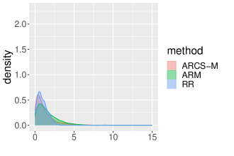
(a) $n=60$, $p=10$.

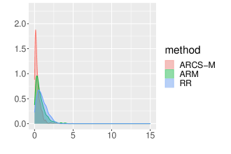
(b) $n=120$, $p=10$.

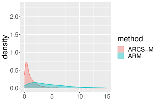
(c) $n=60$, $p=150$.

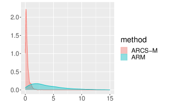
(d) $n=120$, $p=150$.

Figure 1: The simulated distribution of $\text{Imb}_{i,J^{*}}^{M}$ in Example 1.

Table 1: Simulation results for Example 1 (a) with $p=10$: (1) $\text{Imb}_{n,J^{*}}^{M}$; (2) $\tau$: mean and $\sqrt{n}\times$standard deviation ($\sqrt{n}$s.d.) and (3) computation time (in seconds).

	$n$	CR	RR	ARM	ARCS-M
					$N=2$	$N=10$
$\text{Imb}_{n,J^{*}}^{M}$	60	5.82	0.97	1.63	1.27	1.10
	120	5.86	0.96	0.76	0.41	0.39
$\tau$: mean ($\sqrt{n}$s.d.)	60	1.06 (9.34)	1.02 (4.09)	0.98 (5.20)	0.98 (4.53)	0.99 (4.60)
	120	0.98 (9.20)	0.98 (4.19)	0.99 (3.82)	1.00 (3.21)	1.00 (3.02)
time (s)	60	0.00	0.11	0.13	1.97	0.50
	120	0.00	0.08	0.18	5.22	1.20

Table 2: Simulation results Example 1 (b) with for $p=150$: (1) $\text{Imb}_{n,J^{*}}^{M}$; (2) $\tau$: mean and $\sqrt{n}\times$standard deviation ($\sqrt{n}$s.d.) and (3) computation time (in seconds).

	$n$	CR	ARM	ARCS-M
				$N=2$	$N=10$
$\text{Imb}_{n,J^{*}}^{M}$	60	5.94	4.47	1.12	1.17
	120	6.21	4.16	0.34	0.34
$\tau$: mean ($\sqrt{n}$s.d.)	60	1.00 (9.47)	1.04 (7.95)	0.98 (4.42)	0.98 (4.34)
	120	1.01 (9.72)	1.02 (7.69)	0.99 (2.95)	1.00 (2.94)
time (s)	60	0.00	1.62	2.39	0.55
	120	0.00	3.23	7.63	1.77

The superiority of ARCS-M is evident in three key aspects, as shown in Tables 1 and 2. Firstly, in terms of covariate imbalance measured by $\text{Imb}_{n,J^{*}}^{M}$, ARCS-M consistently outperforms its competitors (in both low-dimensional and high-dimensional settings, with $n=60$ or $n=120$), with the only exception in $n=60,p=10$ where ARCS-M is slightly worse than RR. The advantage is more evident in the high-dimensional case where $p=150$, as ARCS-M reduces the imbalance to only 25% and 10% of that of ARM (and CR) when $n=60$ and $n=120,$ respectively. Secondly, as shown in panel (a) of Figure 3, the variable selection step successfully identifies all three influential covariates ($J^{*}$) even with a small sample size of $30$ (after 1st batch), resulting in a true positive rate of 1 on average. On the other hand, with $s=3$ influential covariates and $p=10$, a false-positive rate of 0.25 indicates an average selection of 1.75 non-influential covariates. Thus, on average, ARCS-M balances 4.75 covariates while its competitors balance all 10 covariates. When $p=150$, panel (b) of Figure 3 reports a true positive rate of 1 after around 10 batches, and a 0 false positive rate consistently. This means ARCS-M can balance on exactly the 3 truly important covariates rather than 150 covariates as done in other competing methods. By focusing on a smaller set of covariates covering $J^{*}$, thanks to the additional covariate selection step, ARCS-M mitigates the issue of over-incorporation of covariates, resulting in superior performance in terms of balancing the underlying influential set $J^{*}$. Thirdly, ARCS-M achieves smaller standard errors of the estimated treatment effect compared to its competitors in general, and the improvement is more pronounced with increasing sample size ($n$). While ARCS-M with $N=2$ may be slower than ARM due to the additional Lasso step, increasing the batch size to $N=10$ significantly reduces computational time. Therefore, for users with limited computational resources, choosing a slightly larger batch size can substantially reduce computation time without sacrificing efficiency, as demonstrated in both Tables 1 and 2.

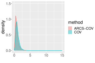
(a) $n=60$, $p=10$.

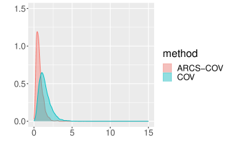
(b) $n=120$, $p=10$.

(c) $n=60$, $p=150$.

(d) $n=120$, $p=150$.

Figure 2: The simulated distribution of $\text{Imb}_{i,J^{*}}^{\phi}/100$ in Example 1.

Table 3: Simulation results for Example 1 (a) with $p=10$ : (1) DNCM; (2) DNC; (3) $\text{Imb}_{n,J^{*}}^{\phi}$; (4) $\tau$: mean and $\sqrt{n}\times$standard deviation in Special case 2 and (5) computation time (in seconds).

	$n$	CR	COV	ARCS-COV
				$N=1$	$N=10$
DNCM	60	718.78	133.09	132.09	131.84
	120	1453.19	147.20	108.92	106.56
DNC	60	3023.38	1678.61	1365.60	1387.96
	120	5999.52	2522.13	1286.70	1261.87
$\text{Imb}_{n,J^{*}}^{\phi}$	60	308.76	101.92	79.20	80.44
	120	620.76	141.22	72.02	71.70
$\tau$: mean ($\sqrt{n}$s.d.)	60	0.99 (9.32)	1.00 (4.07)	1.00 (4.09)	1.00 (4.05)
	120	0.99 (9.56)	1.00 (3.23)	1.00 (3.04)	1.00 (3.02)
time (s)	60	0.00	0.00	3.53	0.46
	120	0.00	0.01	7.83	0.81

Table 4: Simulation results for Example 1(b) with $p=150$: (1) DNCM; (2) DNC; (3) $\text{Imb}_{n,J^{*}}^{\phi}$; (4) $\tau$: mean and $\sqrt{n}\times$standard deviation in Special case 2 and (5) computation time (in seconds).

	$n$	CR	COV	ARCS-COV
				$N=1$	$N=10$
DNCM	60	726.54	388.97	139.97	155.55
	120	1430.37	600.13	103.25	104.17
DNC	60	3043.94	3002.91	1412.86	1453.88
	120	6064.75	5968.93	1153.76	1203.63
$\text{Imb}_{n,J^{*}}^{\phi}$	60	310.87	231.08	82.08	87.90
	120	622.20	422.87	65.14	67.20
$\tau$: mean ($\sqrt{n}$s.d.)	60	1.01 (9.37)	0.98 (6.64)	1.01 (4.16)	1.00 (4.27)
	120	1.01 (9.35)	1.01 (5.77)	1.00 (3.04)	0.99 (2.98)
time (s)	60	0.00	0.04	5.98	0.47
	120	0.00	0.09	13.47	1.69

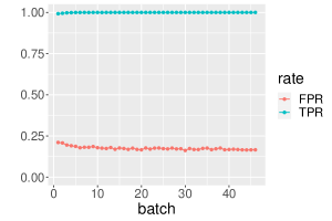
(a) ARCS-M, $n=120$, $p=10$.

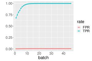
(b) ARCS-M, $n=120$, $p=150$.

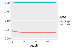
(c) ARCS-COV, $n=120$, $p=10$.

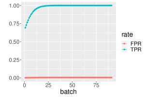
(d) ARCS-COV, $n=120$, $p=150$.

Figure 3: True positive rate and false positive rate for covariates selection in Example 1.

Similar messages for ARCS-COV have been conveyed in Tables 3 and 4. Additionally, we present results on DNCM and DNC (defined at the beginning of this section) following the methodology outlined in Ma et al., (2024). Although these quantities are not the primary focus of ARCS-COV, the numerical results indicate that ARCS-COV consistently outperforms COV in all scenarios. Specifically, for cases with $n=120,p=10$ and $n=120,p=150$, the DNC achieved by ARCS-COV is only approximately 50% and 20% of that attained by COV, respectively. Similarly, for cases with $n=60,p=150$ and $n=120,p=150$ in Table 4, the DNCM achieved by ARCS-COV is only about 35% and 18% of that obtained by COV, indicating significant reductions in those metrics.

When comparing the results between low-dimensional settings with $p=10$ (Tables 1 and 3) and high-dimensional settings with $p=150$ (Tables 2 and 4), we observe that the performance of ARCS-M and ARCS-COV remains largely unchanged, while the performance of the competitors deteriorates rapidly. Figure 1 and 2 deliver similar messages. There are two potential explanations for this observation: 1) The estimation of the precision matrix is crucial for the implementation of ARM. When the number of covariates ($p$) exceeds the sample size ($n$), incorporating all covariates can lead to either an invalid inverse of a low-rank matrix or inaccurate results when using the generalized inverse of $\widehat{\Sigma}$. ARCS-M is not affected since the number of selected covariates is smaller than $n$ in general; 2) Both ARM and COV tend to incorporate more unimportant covariates, which reduces the emphasis on balancing the important covariates. Specifically, COV balances all $p=150$ covariates, while ARCS-COV balances only the 3 true covariates. As a result, the issue of over-incorporation of non-influential covariates worsens as $p$ increases from 10 to 150.

Example 2 (A combination of continuous and discrete covariates).

In accordance with the basic setups outlined in Example 1, we introduce a modification by replacing the last four continuous covariates with discrete covariates. Specifically, we start by generating i.i.d. $Z_{i1}$, $Z_{i2}\sim\text{Bernoulli}(0.5)$ for $1\leq i\leq n$. Subsequently, we construct a set of discrete covariates by considering the four-way combinations of indicator functions involving $Z_{i1}$ and $Z_{i2}$, as described in the outcome model (4.2). The remaining covariates and random noises are generated following Example 1, while maintaining the dimension $p$ unchanged. The updated outcome model can be represented as

$$Y_{i}=\mu(1)T_{i}+\mu(0)(1-T_{i})+X_{i}^{\top}\beta^{*}+\varepsilon_{i},$$ (4.2)

where the first $p-4$ coordinates of $X_{i}$ remain unchanged, $x_{i,p-3}={\rm 1}\kern-2.40005pt{\rm I}(Z_{i1}=1,Z_{i2}=1)$, $x_{i,p-2}={\rm 1}\kern-2.40005pt{\rm I}(Z_{i1}=1,Z_{i2}=0)$, $x_{i,p-1}={\rm 1}\kern-2.40005pt{\rm I}(Z_{i1}=0,Z_{i2}=1)$ and $x_{ip}={\rm 1}\kern-2.40005pt{\rm I}(Z_{i1}=0,Z_{i2}=0)$. Moreover, we choose $\beta^{*}=(3,1.5,0,0,2,\mathbf{0}_{p-9}^{\top},1,0,0,0)^{\top}$, thus beyond the three influential continuous covariates, we have one more influential discrete covariate that contributes to the response $Y$. Since we have demonstrated the effect of varying sample size $n$ in Example 1, we will examine only ARCS-COV, keeping $n=120$ and varying $p=\{10,150\}$, with $s=4$.

We present the results in Table 5. It is evident that when $p=150$, ARCS-COV achieves a remarkable improvement over COV, reducing all three metrics to at most 30% of their corresponding values generated by COV. Notably, CR remains the poorest performing method across all approaches. On the other hand, when $p=10$, while the performance of ARCS-COV in terms of the DNCM is comparable to that of COV, ARCS-COV still outperforms its competitors in terms of the other two metrics. Therefore, Example 2 demonstrates that ARCS is applicable not only to the selection of continuous covariates but also to a mixture of continuous and discrete covariates. Furthermore, the average TPR and FPR of the last batch is $99.06\%$ and $22.94\%$ respectively when $n=120$, $p=10$; and the corresponding values are $91.71\%$ and $0.68\%$ when $n=120$, $p=150$. The results clearly indicate that, in both cases, we incorporate an average of only 1 non-influential covariate into our model ($22.94\%\times 6=1.38$ and $0.68\%\times 146=0.99$). This effectively addresses the problem of covariate over-incorporation. Moreover, the average true positive rates exceed 99% and 91%, demonstrating that ARCS reliably captures all the influential covariates.

Table 5: Simulation results for Example 2: (1) DNCM; (2) DNC; (3) $\text{Imb}_{n,J^{*}}^{\phi}$ in Special case 2; (4) $\tau$: mean and $\sqrt{n}\times$standard deviation and (5) computation time (in seconds).

	$p$	CR	COV	ARCS-COV
				$N=1$	$N=10$
DNCM	10	1572.69	111.10	113.21	117.20
	150	1510.91	668.13	165.04	164.22
DNC	10	6909.01	2331.25	1736.38	1711.03
	150	6963.59	6586.54	1854.04	1855.22
$\text{Imb}_{n,J^{*}}^{\phi}$	10	640.62	111.24	82.90	83.49
	150	632.19	408.33	97.75	98.59
$\tau$: mean ($\sqrt{n}$s.d.)	10	0.99 (9.77)	0.99 (2.91)	1.01 (2.92)	1.00 (2.95)
	150	1.01 (9.30)	1.00 (5.81)	1.00 (3.10)	1.00 (3.06)
time (s)	10	0.00	0.00	7.11	0.78
	150	0.00	0.11	9.91	1.09

Since Example 1 has been thorough in exploring various settings, including small and large sample sizes, as well as low and high dimensions, in Examples 3 and 4, we will focus on a single setting in terms of $n=300$ and $p=150$ to deliver a more focused message.

Example 3.

We consider a nonlinear outcome model, utilizing $f_{1}(x)$, $f_{2}(x)$, $f_{3}(x)$ and $f_{4}(x)$ which represent sine, polynomial and exponential functions. Specifically,

$$Y_{i}=\mu(1)T_{i}+\mu(0)(1-T_{i})+f_{1}(x_{i1})+f_{2}(x_{i2})+f_{3}(x_{i3})+f_{4}(x_{i4})+\varepsilon_{i},$$

with $f_{1}(x)=-2\sin(2x),\quad f_{2}(x)=x^{2}-\frac{1}{3},\quad f_{3}(x)=x-\frac{1}{2},\quad f_{4}(x)=e^{-x}+e^{-1}-1\,.$ The covariates and random noises are generated similarly as in Example 1 .

Table 6: Simulation results for Example 3: (1) $\text{Imb}_{n,J^{*}}^{M}$; (2) DNCM; (3) DNC; (4) $\text{Imb}_{n,J^{*}}^{\phi}$ in Special case 2 and (5) $\tau$: mean and $\sqrt{n}\times$ standard deviation.

	CR	ARM	ARCS-M-add	COV	ARCS-COV-add
$\text{Imb}_{n,J^{*}}^{M}$	8.00	5.16	1.23	-	-
DNCM	4686.11	-	-	1177.82	567.72
DNC	26754.32	-	-	23811.09	11273.14
$\text{Imb}_{n,J^{*}}^{\phi}$	2217.85	-	-	1255.95	538.76
$\tau$: mean ($\sqrt{n}$s.d.)	1.00 (6.20)	1.00 (5.66)	1.00 (5.15)	1.01 (5.28)	1.01 (4.66)

From Table 6, ARCS-M-add reduces the Mahalanobis distance to 16% and 24% of the values achieved by CR and ARM, respectively. Further, ARCS-COV-add method reduces all the three measures DNCM, DNC, and $\text{Imb}_{n,J^{*}}^{\phi}$ to at most 50% of the values achieved by COV. Thus overall, ARCS-M-add and ARCS-COV-add are effective in balancing the important covariates when the outcome model is nonlinear.

Example 4.

We choose the following outcome model such that it matches the choice of $\phi$ in COV.The covariates and random noises are generated similarly as in Example 1.

$$Y_{i}=\mu(1)T_{i}+\mu(0)(1-T_{i})+3x_{i1}+3x_{i2}+3x_{i1}^{2}+3x_{i2}^{2}+3x_{i1}x_{i2}+\varepsilon_{i}.$$

Table 7 presents a three-fold message. First, when the underlying outcome model matches the choice of $\phi$ that defines the imbalance measure in the CAR procedure, both ARCS-COV and ARCS-COV-add significantly improve the inference result by reducing the standard error of the estimated treatment effect to approximately half. COV is expected to perform well in this setting, as stated in Ma et al., (2024), but it appears to underperform because the outcome model (defined with only $x_{i1}$ and $x_{i2}$) does not match the $\phi$ that is defined on all $p=150$ covariates without selection. Second, in terms of DNCM, ARCS-COV mildly improves the results compared to COV, while ARCS-COV-add directly reduces the DNCM measure to less than 27% of the value obtained with COV. This illustrates the advantage of utilizing the sparse additive models. Third, in terms of the DNC and $\text{Imb}_{n,J^{*}}^{\phi}$ metrics, both ARCS-COV and ARCS-COV-add outperforms COV and CR by reducing the metrics to less than 28% of the values obtained with their competitors, with ARCS-COV-add performs comparatively better. This suggests that the key improvement in reducing DNC and $\text{Imb}_{n,J^{*}}^{\phi}$ is primarily due to the covariate selection step.

Table 7: Simulation results over 5000 repetitions in Example 4, comparing the performances of CR, COV, ARCS-COV and ARCS-COV-add under a nonlinear outcome model matching $\phi$ in COV.

	CR	COV	ARCS-COV	ARCS-COV-add
DNCM	2508.21	602.80	565.41	160.24
DNC	8625.14	8290.49	1926.34	1740.01
$\text{Imb}_{n,J^{*}}^{\phi}$	1182.76	617.95	178.73	112.53
$\tau$: mean ($\sqrt{n}$s.d.)	0.95 (7.79)	0.98 (7.41)	0.99 (3.43)	1.03 (3.63)

5 An Example based on Clinical Trial Study

We present an extensive analysis of an illustrative clinical trial study to highlight the advantages of ARCS over other existing methods without a covariate selection step, in terms of covariate balancing and treatment effect estimation. The concerned randomized clinical trial was originally conducted to compare the effectiveness of three treatments for chronic depression: nefazodone, the cognitive behavioral-analysis system of psychotherapy, and their combination (Keller et al.,, 2000). As we aim to address the scenario involving two treatments in this paper, we will focus only on the data related to the nefazodone treatment and the combination treatment following Ma et al., (2024). In this study, the outcome variable $Y$ of interest is the 24-item Hamilton Rating Scale for Depression post-treatment, specifically the last observed score (referred to as FinalHAMD). We consider all 57 informative covariates in the dataset, including both discrete and continuous ones, but excluding any meaningless covariates such as the indices. Thus, we work with a dataset of size $n=376$ and $p=57$. We apply 5-fold cross-validated Lasso, and select $s=2$ covariates, namely RACE and HAMD24. We consider the following two outcome models, one is linear and the other is quadratic.

$$\text{{\sf Linear:}}\text{ FinalHAMD}_{i}=\mu(1)T_{i}+\mu(0)(1-T_{i})+\beta_{1}^{*}\text{RACE}_{i}+\beta_{2}^{*}\text{HAMD24}_{i}+\varepsilon_{i}.$$ (5.1)

$$\text{{\sf Quadratic:}}\text{ FinalHAMD}_{i} =\mu(1)T_{i}+\mu(0)(1-T_{i})+\beta_{1}^{*}\text{RACE}_{i}+\beta_{2}^{*}\text{HAMD24}_{i}$$

$$+\beta_{3}^{*}\text{RACE}_{i}^{2}+\beta_{4}^{*}\text{HAMD24}_{i}^{2}+\beta_{5}^{*}\text{RACE}_{i}\times\text{HAMD24}_{i}+\varepsilon_{i}.$$ (5.2)

We first compute the least-square estimators $(\hat{\mu}(1),\hat{\mu}(0),\hat{\beta})$ based on the original dataset and further get $\hat{\mu}(1)-\hat{\mu}(0)$. Then in each replication, we generate a pseudo dataset based on these estimated parameters and $\varepsilon_{i}\overset{\text{i.i.d.}}{\sim}\mathcal{N}(0,1)$. Numerical results are summarized in Table 8 and Figure 4 based on 5,000 replications.

Table 8: Numerical results for the clinical trial example: comparison across different methods based on both linear and quadratic outcome models.

		CR	ARM	ARCS-M	COV	ARCS-COV
Linear model	$\text{Imb}_{n,J^{*}}^{M}$	3.93	0.88	0.08	-	-
	DNCM$(\times 10^{3})$	38.34	-	-	3.02	0.94
	DNC$(\times 10^{6})$	127.82	-	-	10.02	3.13
	$\text{Imb}_{n,J^{*}}^{\phi}(\times 10^{6})$	64.86	-	-	6.84	1.42
	$\tau$: mean ($\sqrt{n}$s.d.)	-4.33 (5.02)	-4.34 (2.91)	-4.34 (2.06)	-4.34 (2.44)	-4.34 (2.11)
Quadratic model	$\text{Imb}_{n,J^{*}}^{M}(\times 10^{6})$	4.05	0.91	0.15	-	-
	DNCM$(\times 10^{3})$	38.8	-	-	3.18	1.47
	DNC$(\times 10^{6})$	129.79	-	-	10.47	4.94
	$\text{Imb}_{n,J^{*}}^{\phi}(\times 10^{6})$	63.35	-	-	6.81	3.43
	$\tau$: mean ($\sqrt{n}$s.d.)	-4.48 (5.61)	-4.47 (3.62)	-4.48 (3.17)	-4.47 (2.87)	-4.48 (2.30)

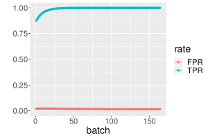
(a) ARCS-M, Linear model.

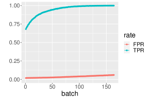
(b) ARCS-M, Quadratic model.

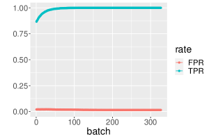
(c) ARCS-COV, Linear model.

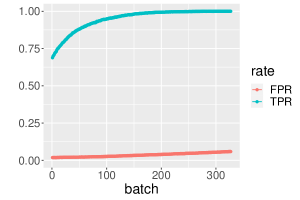
(d) ARCS-COV, Quadratic model.

Figure 4: True positive rate and false positive rate for covariates selection in the clinical trial example.

Figure 4 demonstrates the advanced performance of the covariate selection step used in ARCS. For both the linear and the quadratic models, Figure 4 indicates that ARCS-M and ARCS-COV control the false positive rate under 10% or less, and their true positive rates reach 1 once the accumulated sample size exceeds $n/2$ or even earlier. Consequently, it ensures the significant covariates are selected and used for balancing in ARCS-M or ARCS-COV.

Thanks to the reduced dimension of covariates, both ARCS-M and ARCS-COV can improve the balance of the significant covariates and further enhance the efficiency of the treatment effect estimation. Examining first the results from ‘Linear model’ in Table 8, we observe that both ARCS-M and ARCS-COV significantly reduce the covariate imbalance and the standard error of $\hat{\tau}$, compared to their counterparts ARM and COV, not to mention CR which has the poorest performance consistently. This demonstrates the effect of the extra covariate selection step in ARCS. The similar standard errors of $\hat{\tau}$ by ARCS-M and ARCS-COV indicate that when a linear model is used, balancing the covariate means might be sufficient. When we further look at the ‘Quadratic model’ results, where the outcome model matches the selection of $\phi$ in COV, ARCS-COV achieves a scaled standard error of $\hat{\tau}$ of 2.30, while ARCS-M is 3.17. This shows that when the model becomes more sophisticated, balancing higher-order functions of covariates can further improve the estimation of the treatment effect, validating the development of ARCS-COV.

6 Conclusion

In this article, ARCS procedures are proposed to achieve the simultaneous goals of covariates selection and balancing. Importantly, we extend the finite-dimensional covariates framework to compare the balance properties of the CAR without covariate selection and ARCS. Under a high-dimensional covariates setting, we show that the CAR without covariates selection suffers from a slow convergence rate of its imbalance measure, whereas ARCS achieves a much faster convergence rate for the imbalance over the set of true influential covariates. The benefit of ARCS is further demonstrated by showing improved efficiency in estimating the treatment effect from a linear outcome model. We conduct extensive numerical studies to demonstrate the appealing properties of ARCS under various settings.

While our primary focus has been on demonstrating the impact of selecting and balancing covariates on treatment effect estimation, the results presented also yield significant insights into subsequent hypothesis testing. Assuming the linear outcome model (2.1), inference for the treatment effect can be conducted based on Theorem 2 and the estimate based on Lasso regression. However, in practice, the presumed linear outcome models might not accurately capture the data generating process (Liu et al.,, 2022; Ma et al.,, 2022; Gu et al.,, 2023; Ye et al.,, 2021, 2023). Therefore, there is a pressing need to extend the presented framework to develop model-robust inference methods for treatment effects following the application of ARCS.

To understand the balance properties of the CAR procedure, it is desirable to examine the finite-sample performance of the imbalance measure in more detail. In typical clinical trials, it is assumed that baseline covariates are predefined prior to the experiment, with the dimension considered finite as patient enrollment increases (Hu and Hu, 2012a, ; Qin et al.,, 2024; Ma et al.,, 2024). However, integrating electronic health records and other technological advancements can result in a substantial increase in the dimension of covariates available for the design of the trial. When the number of covariates is large, the features used for achieving balance may have an even higher dimension, potentially leading to worse finite-sample performance on covariate balancing. Although Proposition 2 partially addresses this issue by introducing a simplified assumption, more comprehensive and relaxed assumptions are necessary to adequately delineate the structure of the features utilized in the design. Subsequently, detailed evaluations of the finite sample properties should be undertaken to understand better the impacts and efficacy of the balance achieved through CAR in high-dimensional settings.

The fast diverging dimension of the functions of covariates used in CAR demonstrates the need to reduce their dimension in order to improve the performance of covariate balancing. It is thus advantageous to directly select the basis of the functions used in the design with ARCS. However, correlations among the basis of these functionals can introduce complexities in the selection process. To mitigate this challenge, one might consider employing the group lasso technique on blocks of functional elements, particularly when supplementary information facilitates the segmentation of these functionals into independent blocks. It is also of interest to understand the impact of the selection of the functionals with ARCS on the estimation of treatment effect. We leave this problem as a future research topic.

7 Acknowledgements

Yang Liu’s research is supported by the National Natural Science Foundation of China grant 12301324. Lucy Xia’s research is supported by the Hong Kong Research Grants Council ECS grant 26305120.

Appendix A Supplement for ARCS procedure

A.1 Implementation of of ARCS-M

Since $\text{Imb}^{\phi}_{i,J^{*}}$ is proportional to the Mahalanobis distance and $\Sigma_{J^{*}}$ is unknown in practice, we alternatively implement step (3) of ARCS following the procedure in (Qin et al.,, 2024), described as following step (3’).

• Suppose we have assigned $(2i-2)$ units. For $a=0,1$, the imbalance measure via Mahalanobis distance is

  $$\text{Imb}^{M}_{2i,\widehat{J}^{(b-1)}}=(2i/2)(\bar{X}_{2i,\widehat{J}^{(b-1)}}(1)-\bar{X}_{2i,\widehat{J}^{(b-1)}}(0))^{\top}\widehat{\Sigma}_{\widehat{J}^{(b-1)}}^{-1}(\bar{X}_{2i,\widehat{J}^{(b-1)}}(1)-\bar{X}_{2i,\widehat{J}^{(b-1)}}(0))\,,$$

  where $\widehat{\Sigma}_{\widehat{J}^{(b-1)}}$ is the sample covariance matrix calculated by the sample set $\{X_{k,\widehat{J}^{(b-1)}}\}_{k=1}^{2i}$. Let $\text{Imb}^{M}_{2i,\widehat{J}^{(b-1)}}(a)$ be the imbalance measure with $T_{2i-1}=a$, $T_{2i}=1-a$ for $a=0,1$. Let us assign the $(2i-1)$-th unit with probability

  $${\rm I}\kern-1.79993pt{\rm P}\left(T_{2i-1}=1\mid X_{1},\ldots,X_{2i},T_{1},\ldots,,T_{2i-2}\right)=\left\{\begin{array}[]{ll}\rho,&\text{Imb}^{M}_{2i,\widehat{J}^{(b-1)}}(1)<\text{Imb}^{M}_{2i,\widehat{J}^{(b-1)}}(0),\\ 1-\rho,&\text{Imb}^{M}_{2i,\widehat{J}^{(b-1)}}(1)>\text{Imb}^{M}_{2i,\widehat{J}^{(b-1)}}(0),\\ 0.5,&\text{Imb}^{M}_{2i,\widehat{J}^{(b-1)}}(1)=\text{Imb}^{M}_{2i,\widehat{J}^{(b-1)}}(0),\end{array}\right.$$

  where $\rho\in(0.5,1)$, and define $T_{2i}=1-T_{2i-1}$.

A.2 Summary of the ARCS Procedures

Algorithm 1 ARCS Procedure

0:    $X_{1},\dots,X_{n}$: Covariates; $N_{0}$: Initial batch size; $N$: Batch size; $\rho$: The probability of the biased coin.

0:    $T_{1},\dots,T_{n}$: Assignments.

1:  for $i=1$ to $N_{0}$ do

2:     Let $T_{i}=1$ with probability 0.5.

3:  end for

4:  For $a=0,1$, obtain the Lasso estimator

$$(\hat{\mu}^{(0)}(a),(\hat{\beta}^{(0)}(a))^{\top})=\mathop{\arg\min}\limits_{(\mu,\beta)}\left\{\frac{1}{n_{a}^{(0)}}\sum_{1\leq i\leq N_{0}:T_{i}=a}(Y_{i}-\mu-X_{i}^{\top}\beta)^{2}+\lambda_{a}\sum_{j=1}^{p}|\beta_{j}|\right\}\,.$$

5:  Set $\widehat{J}^{(0)}=J(\hat{\beta}^{(0)}(0))\cap J(\hat{\beta}^{(0)}(1))$.

6:  for $b=1$ to $(n-N_{0})/N$ do

7:     for $i=N_{0}+(b-1)N+1$ to $N_{0}+bN$ do

8:        Calculate $\text{Imb}_{i,\widehat{J}^{(b-1)}}(1)$, $\text{Imb}_{i,\widehat{J}^{(b-1)}}(0)$.

9:        if $\text{Imb}_{i,\widehat{J}^{(b-1)}}(1)<\text{Imb}_{i,\widehat{J}^{(b-1)}}(0)$ then

10:           Set $T_{i}=1$ with probability $\rho$.

11:        else if $\text{Imb}_{i,\widehat{J}^{(b-1)}}(1)>\text{Imb}_{i,\widehat{J}^{(b-1)}}(0)$ then

12:           Set $T_{i}=1$ with probability $1-\rho$.

13:        else

14:           Set $T_{i}=1$ with probability 0.5.

15:        end if

16:     end for

17:     For $a=0,1$, obtain the Lasso estimator

$$(\hat{\mu}^{(b)}(a),(\hat{\beta}^{(b)}(a))^{\top})=\mathop{\arg\min}\limits_{(\mu,\beta)}\left\{\frac{1}{n_{a}^{(b)}}\sum_{1\leq i\leq N_{0}+bN:T_{i}=a}(Y_{i}-\mu-X_{i}^{\top}\beta)^{2}+\lambda_{a}\sum_{j=1}^{p}|\beta_{j}|\right\}\,.$$

18:     Set $\widehat{J}^{(b)}=J(\hat{\beta}^{(b)}(0))\cap J(\hat{\beta}^{(b)}(1))$.

19:  end for

20:  return  $T_{1},\dots,T_{n}$.

Appendix B Proof of the Main Results

B.1 Proof of Proposition 1: the selection consistency of Lasso

In this section, we prove the covariate selection consistency of Lasso in Proposition 1. The proof contains two major steps. First, we prove that the Restricted Eigenvalue (RE) condition holds for $\mathbb{X}(a)$ with high probability under Assumption 1(i)(iii) in Lemma 1. Second, we derive the covariate selection consistency based on the RE condition. The second part is based on Bickel et al., (2009).

Let $e_{j}\in\mathbb{R}^{p}$ be the vector with the $j$-th element equal to 1 and all other elements equal to 0. For simplicity of notation, $c^{\prime}$, $C$, $C^{\prime}$ are generic constants that vary from line to line. Lemma 1 provides results for a general $c_{a}$. Later we will apply the result to $c_{a}=3$ in our context.

Lemma 1.

Suppose Assumption 1 (i) and (iii) hold with $c_{a}=3$ replaced by a generic $c_{a}$, for $a\in\{0,1\}$. Further, let $\kappa(s,3c_{a})$ be the value associated with $p^{1/2}A_{a}$ under $\text{RE}(s,3c_{a})$, $\kappa(s,c_{a})$ be the value associated with $p^{1/2}A_{a}$ under $\text{RE}(s,c_{a})$, and set

$$m=\min\left(s+s\max_{1\leq j\leq p}\lVert A_{a}e_{j}\rVert_{2}^{2}\frac{16(3c_{a})^{2}(3c_{a}+1)}{r_{a}^{2}\kappa^{2}(s,3c_{a})},p\right).$$

Suppose

$$n_{a}\geq\frac{2000m\iota^{4}}{r_{a}^{2}}\log\left\{(mr_{a})^{-1}60pe\right\}.$$

Then with probability at least $1-2\exp\{-r_{a}^{2}n_{a}/(2000\iota^{4})\}$, $\mathbb{X}(a)$ satisfies $\text{RE}(s,c_{a})$ condition. Additionally, if we denote $\kappa_{\mathbb{X}(a)}(s,c_{a})$ as the value of $\kappa(\cdot,\cdot)$ associated with $\mathbb{X}(a)$ under $\text{RE}(s,c_{a})$, then

$$\kappa_{\mathbb{X}(a)}(s,c_{a})\geq(1-r_{a})\kappa(s,c_{a})>0.$$

Lemma 1 is a direct consequence of Theorem 6 in Rudelson and Zhou, (2012), we thus omit the proof. The following lemma provides a key step used in the proof of Proposition 1.

Lemma 2.

Under Assumption 1 (i) and (ii), for group $a\in\{0,1\}$, let

$$\lambda_{a}=2c\sigma_{\varepsilon}\max\left(\sqrt{\frac{(1+\alpha)\log n_{a}+\log(2p)}{\xi_{a}n_{a}}},\frac{(1+\alpha)\log n_{a}+\log(2p)}{\xi_{a}n_{a}}\right)\,,$$

then with probability at least $1-n_{a}^{-(1+\alpha)}$, for all $\beta\in\mathbb{R}^{p}$,

$$\quad\frac{1}{n_{a}}\lVert\mathbb{X}(a)(\hat{\beta}(a)-\beta^{*})\rVert_{2}^{2}+\lambda_{a}\sum_{j=1}^{p}|\hat{\beta}_{j}(a)-\beta_{j}|$$

$$\leq\frac{1}{n_{a}}\lVert\mathbb{X}(a)(\beta-\beta^{*})\rVert_{2}^{2}+4\lambda_{a}\sum_{j\in J(\beta)}|\hat{\beta}_{j}(a)-\beta_{j}|$$ (B.1)

$$\leq\frac{1}{n_{a}}\lVert\mathbb{X}(a)(\beta-\beta^{*})\rVert_{2}^{2}+4\lambda_{a}\sqrt{|J(\beta)|}\sqrt{\sum_{j\in J(\beta)}|\hat{\beta}_{j}(a)-\beta_{j}|^{2}}.$$ (B.2)

Proof of Lemma 2.

Without loss of generality, suppose $Y$ is centralized. By the definition of Lasso, for all $\beta\in\mathbb{R}^{p}$ and group $a=0,1$, we have

$$\frac{1}{n_{a}}\lVert Y-\mathbb{X}(a)\hat{\beta}(a)\rVert_{2}^{2}+2\lambda_{a}\sum_{j=1}^{p}|\hat{\beta}_{j}(a)|\leq\frac{1}{n_{a}}\lVert Y-\mathbb{X}(a)\beta\rVert_{2}^{2}+2\lambda_{a}\sum_{j=1}^{p}|\beta_{j}|\,.$$

Since $Y=\mathbb{X}\beta^{*}+\varepsilon$, it follows that

$$\quad\frac{1}{n_{a}}\lVert\mathbb{X}(a)(\beta^{*}-\hat{\beta}(a))\rVert_{2}^{2}+2\lambda_{a}\sum_{j=1}^{p}|\hat{\beta}_{j}(a)|$$

$$\leq\frac{1}{n_{a}}\lVert\mathbb{X}(a)(\beta^{*}-\beta)\rVert_{2}^{2}+2\lambda_{a}\sum_{j=1}^{p}|\beta_{j}|+\frac{2}{n_{a}}\varepsilon^{\top}\mathbb{X}(a)(\hat{\beta}(a)-\beta)\,.$$ (B.3)

Define the event

$$\mathcal{A}_{a}=\bigcap_{j=1}^{p}\left\{\frac{2}{n_{a}}\left|\sum_{i:T_{i}=a}\varepsilon_{i}x_{ij}\right|\leq\lambda_{a}\right\}\,,\quad a\in\{0,1\},$$

By Assumption 1 (i) and (ii), we obtain $\lVert x_{ij}\rVert_{\psi_{2}}\leq C^{\prime}$ for some constant $C^{\prime}$. It follows from Lemma 2.7.7. of Vershynin, (2018) that $\varepsilon_{i}x_{ij}$ is sub-exponential with

$$\lVert\varepsilon_{i}x_{ij}\rVert_{\psi_{1}}\coloneq\inf\{t>0:{\rm I}\kern-1.79993pt{\rm E}[\exp(|\varepsilon_{i}x_{ij}|/t)]\leq 2\}\leq C^{\prime}L\sigma_{\varepsilon}.$$

Therefore, by Bernstein’s inequality, i.e., Corollary 2.8.3 in Vershynin, (2018), it follows that

$${\rm I}\kern-1.79993pt{\rm P}(\mathcal{A}_{a}^{c}) \leq\sum_{j=1}^{p}{\rm I}\kern-1.79993pt{\rm P}\left(\frac{2}{n_{a}}\left|\sum_{i:T_{i}=a}\varepsilon_{i}x_{ij}\right|>\lambda_{a}\right)$$

$$\leq 2p\exp\left(-\xi_{a}n_{a}\min\left(\frac{\lambda_{a}^{2}}{4L^{2}(C^{\prime})^{2}\sigma^{2}_{\varepsilon}},\sqrt{\frac{\lambda_{a}^{2}}{4L^{2}(C^{\prime})^{2}\sigma^{2}_{\varepsilon}}}\right)\right)$$

$$=n_{a}^{-(1+\alpha)}.$$

Then, on the event $\mathcal{A}_{a}$, equation (B.1) can be rewritten as

$$\quad\frac{1}{n_{a}}\lVert\mathbb{X}(a)(\hat{\beta}(a)-\beta^{*})\rVert_{2}^{2}+\lambda_{a}\sum_{j=1}^{p}|\hat{\beta}_{j}(a)-\beta_{j}|$$

$$\leq\frac{1}{n_{a}}\lVert\mathbb{X}(a)(\beta-\beta^{*})\rVert_{2}^{2}+2\lambda_{a}\sum_{j=1}^{p}(|\hat{\beta}_{j}(a)-\beta_{j}|+|\beta_{j}|-|\hat{\beta}_{j}(a)|)$$

$$\leq\frac{1}{n_{a}}\lVert\mathbb{X}(a)(\beta-\beta^{*})\rVert_{2}^{2}+4\lambda_{a}\sum_{j\in J(\beta)}|\hat{\beta}_{j}(a)-\beta_{j}|,$$

yielding the conclusion of (B.2). This completes the proof of this lemma. ∎

Next we prove Proposition 1 based on Lemma 1 with $c_{a}=3$ and Lemma 2.

Proposition 1 (Covariate selection consistency).

Under Assumption 1 (i)-(iii) with the defined constants, for $a\in\{0,1\}$, let the penalty parameter satisfy

$$\lambda_{a}=2c\sigma_{\varepsilon}\max\left(\sqrt{\frac{(1+\alpha)\log n_{a}+\log(2p)}{\xi_{a}n_{a}}},\frac{(1+\alpha)\log n_{a}+\log(2p)}{\xi_{a}n_{a}}\right)\,,$$

Then, when $n_{a}>C\log(p)$, with probability at least $1-n_{0}^{-1-\alpha}-n_{1}^{-1-\alpha}-2\exp\{-C_{0}n_{0}\}-2\exp\{-C_{1}n_{1}\}$,

$$\widehat{J}\coloneq\bigcap_{a\in\{0,1\}}\left\{j:|\hat{\beta}_{j}(a)|\geq l_{\beta}\right\}=J^{*}\,,$$ (B.4)

where $C$, $C_{0}$ and $C_{1}$ are some positive constants depending on $\iota$, $r_{0}$ and $r_{1}$ in the assumptions.

Proof of Proposition 1.

Let $\delta(a)=\hat{\beta}(a)-\beta^{*}$, and set $\beta=\beta^{*}$ for (B.1) and (B.2). It follows from (B.1) that $\lVert\delta_{(J^{*})^{c}}(a)\rVert_{1}\leq 3\lVert\delta_{J^{*}}(a)\rVert_{1}$, and thus $\lVert\delta(a)\rVert_{1}\leq 4\lVert\delta_{J^{*}}(a)\rVert_{1}\leq 4\sqrt{s}\lVert\delta_{J^{*}}(a)\rVert_{2}$. On the event $\mathcal{A}_{a}$ in the proof of Lemma 2, we have

$$\frac{1}{n_{a}}\lVert\mathbb{X}(a)\delta(a)\rVert_{2}^{2}\leq 4\lambda_{a}\sqrt{s}\lVert\delta_{J^{*}}(a)\rVert_{2}\,.$$

Taking $c_{a}=3$ for Lemma 1, it follows that $\lVert\delta_{J^{*}}(a)\rVert_{2}\leq 4\lambda_{a}\sqrt{s}/((1-r_{a})\kappa(s,3))^{2}$, and it further yields

$$\lVert\hat{\beta}(a)-\beta^{*}\rVert_{1}\leq l_{\beta}\,.$$ (B.5)

In addition, by Assumption 1 (iii) and the fact that

$$\lVert\hat{\beta}(a)-\beta^{*}\rVert_{1}=\sum_{j\notin J^{*}}|\hat{\beta}(a)|+\sum_{j\in J^{*}}|\hat{\beta}(a)-\beta^{*}|,$$

it follows that $\max_{j\notin J^{*}}|\hat{\beta}_{j}(a)|\leq l_{\beta}$, and $\min_{j\in J^{*}}|\hat{\beta}_{j}(a)|\geq l_{\beta}$. Thus, on the intersection of $\mathcal{A}_{0}$, $\mathcal{A}_{1}$, and the event that $\mathbb{X}(0)$ and $\mathbb{X}(1)$ satisfy $\text{RE}(s,3)$, we have (B.4). By Lemma 1 and 2, this event has probability at least $1-n_{1}^{-1-\alpha}-n_{0}^{-1-\alpha}-2\exp\{-r_{0}^{2}n_{0}/(2000\iota^{4})\}-2\exp\{-r_{1}^{2}n_{1}/(2000\iota^{4})\}$, which completes the proof for Proposition 1. ∎

B.2 Proof of Theorem 1: the convergence rate of imbalance measure

In this section, we present the proof of Theorem 1, Corollary 1, and Proposition 1.

Theorem 1.

Suppose Assumptions 1 (i) - (iv) hold and ARCS is used, then ${\rm I}\kern-1.79993pt{\rm E}(\lVert\Lambda_{n,J^{*}}\rVert_{2}^{2})=O(n^{\frac{1}{\gamma-1}}s_{\phi}^{\frac{2\gamma-3}{\gamma-1}})$ and $\Lambda_{n,J^{*}}=O_{p}(n^{\frac{1}{2(\gamma-1)}}s_{\phi}^{\frac{2\gamma-3}{2\gamma-2}})$. Further, if ${\rm I}\kern-1.79993pt{\rm E}(\lVert\phi(X_{i,J^{*}})\rVert_{2}^{\gamma})=O(s_{\phi}^{\frac{\gamma}{2}})$ for all $\gamma>2$, then $\Lambda_{n,J^{*}}=O_{p}(n^{\epsilon}s^{1-\epsilon}_{\phi})$ for any small $\epsilon>0$.

Proof of Theorem 1.

The outline for the proof is as follows. By the selection consistency of Lasso, we can divide the patients who have already been assigned into two parts. The first part consists of finite number of patients at the beginning whose covariates are inadequately selected, resulting in over-incorporation or under-incorporation of balancing. The second part consists of those patients whose covariates are consistently selected and balanced by ARCS. Then, for the first part of the patients, we derive the rate of the imbalance measure. Finally, based on Ma et al., (2024), we establish another rate of the imbalance measure for the second part of the patients, depending on both $n$ and $s_{\phi}$.

Recall $b_{n}=\lfloor(n-N_{0})/N\rfloor$. Define the event $\mathcal{B}_{n}:=\{\widehat{J}^{(b_{n})}=J^{*}\}$ and its complement $\mathcal{B}_{n}^{c}$.

Step 1: By Proposition 1, it follows that

$${\rm I}\kern-1.79993pt{\rm P}(\mathcal{B}_{n}^{c})\leq n_{0}^{-(1+\alpha)}+n_{1}^{-(1+\alpha)}+2\exp(-C_{0}n_{0})+2\exp(-C_{1}n_{1}),$$

which implies $\sum_{n=1}^{\infty}{\rm I}\kern-1.79993pt{\rm P}(\mathcal{B}_{n}^{c})<\infty.$ By the Borel-Cantelli lemma, we have

$${\rm I}\kern-1.79993pt{\rm P}(\mathcal{B}_{n}^{c}\text{ infinitly often})={\rm I}\kern-1.79993pt{\rm P}(\text{for any }m,\text{ there exists }n>m,\mathcal{B}_{n}^{c})=0.$$

In other words, with probability 1, there exists $m_{0}$, for all $n>m_{0}$, $\mathcal{B}_{n}$ holds. For this $m_{0}$, we decompose $\Lambda_{n,J^{*}}$ into two parts,

$$\Lambda_{n,J^{*}}=\Lambda_{m_{0},J^{*}}+\sum_{i=m_{0}+1}^{n}(2T_{i}-1)\phi(X_{i,J^{*}}).$$ (B.6)

The remaining part of the proof is to derive the rates of the two terms in (B.6).

Step 2: For the first term in (B.6), we have

$${\rm I}\kern-1.79993pt{\rm E}\lVert\Lambda_{m_{0},J^{*}}\rVert_{2}^{2} ={\rm I}\kern-1.79993pt{\rm E}\left\{\sum_{1\leq i,k\leq m_{0}}(2T_{i}-1)(2T_{k}-1)(\phi(X_{i,J^{*}}))^{\top}\phi(X_{k,J^{*}})\right\}$$

$$\leq\sum_{i=1}^{m_{0}}{\rm I}\kern-1.79993pt{\rm E}\lVert\phi(X_{i,J^{*}})\rVert_{2}^{2}+\sum_{1\leq i,k\leq m_{0}:i\neq k}{\rm I}\kern-1.79993pt{\rm E}\{(\phi(X_{i,J^{*}}))^{\top}\phi(X_{k,J^{*}})\}$$

$$\leq C_{1}s_{\phi}$$ (B.7)

for some constant $C_{1}$ that does not depend on $n$. The last inequality in (B.2) follows from Assumption 1 (iv).

Step 3: Note that when $n>m_{0}$, by the law of total expectation,

$${\rm I}\kern-1.79993pt{\rm E}(\cdot)={\rm I}\kern-1.79993pt{\rm E}(\cdot\mid\mathcal{B}_{n}){\rm I}\kern-1.79993pt{\rm P}(\mathcal{B}_{n})+{\rm I}\kern-1.79993pt{\rm E}(\cdot\mid\mathcal{B}_{n}^{c}){\rm I}\kern-1.79993pt{\rm P}(\mathcal{B}_{n}^{c})={\rm I}\kern-1.79993pt{\rm E}(\cdot\mid\mathcal{B}_{n}).$$

For brevity, the expectations in the sequel are all conditional on the event $\mathcal{B}_{n}$. We will start with an elementary inequality by Taylor’s expansion as follows. For $\gamma\geq 2$, and any vectors $u$ and $v$, we have

$$\lVert u+v\rVert_{2}-\lVert u\rVert_{2}\leq\gamma u^{\top}v\lVert u\rVert_{2}^{\gamma-2}+c_{\gamma}(\lVert v\rVert^{\gamma}_{2}+\lVert v\rVert^{2}_{2}\lVert u\rVert_{2}^{\gamma-2})$$ (B.8)

for some constant $c_{\gamma}$. Denote the second term in (B.6) as $\Lambda_{m_{0}:n,J^{*}}$. Substitute the decomposition $\Lambda_{m_{0}:(n+1),J^{*}}=\Lambda_{m_{0}:n,J^{*}}+(2T_{n+1}-1)\phi(X_{n+1,J^{*}})$ into (B.8), it follows that

$$\lVert\Lambda_{m_{0}:(n+1),J^{*}}\rVert_{2}^{\gamma}-\lVert\Lambda_{m_{0}:n,J^{*}}\rVert_{2}^{\gamma} \leq\gamma(2T_{n+1}-1)\Lambda_{m_{0}:n,J^{*}}^{\top}\phi(X_{n+1,J^{*}})\lVert\Lambda_{m_{0}:n,J^{*}}\rVert_{2}^{\gamma-2}$$

$$\quad+c_{\gamma}(\lVert\phi(X_{n+1,J^{*}})\rVert_{2}^{\gamma}+\lVert\phi(X_{n+1,J^{*}})\rVert_{2}^{2}\lVert\Lambda_{m_{0}:n,J^{*}}\rVert_{2}^{\gamma-2}).$$ (B.9)

By some calculations, we have $\text{Imb}_{n,J^{*}}^{\phi}(1)-\text{Imb}_{n,J^{*}}^{\phi}(0)=4\Lambda_{n,J^{*}}^{\top}\phi(X_{n+1,J^{*}})$. Then, under ARCS, we have

$$\quad{\rm I}\kern-1.79993pt{\rm E}((2T_{n+1}-1)\Lambda_{m_{0}:n,J^{*}}^{\top}\phi(X_{n+1,J^{*}})\mid X_{n+1},\dots,X_{1},T_{n},\dots,T_{1})$$

$$={\rm I}\kern-1.79993pt{\rm E}((2T_{n+1}-1)(\Lambda_{n,J^{*}}-\Lambda_{m_{0},J^{*}})^{\top}\phi(X_{n+1,J^{*}})\mid X_{n+1},\dots,X_{1},T_{n},\dots,T_{1})$$

$$\leq-(2\rho-1)|\Lambda_{n,J^{*}}^{\top}\phi(X_{n+1,J^{*}})|+cs_{\phi}$$ (B.10)

for some constant $c$. Taking the conditional expectation ${\rm I}\kern-1.79993pt{\rm E}(\cdot\mid\Lambda_{n,J^{*}})$ on both sides of (B.2), by inequality (B.2) and Assumption 1 (iv), we obtain

$$\quad{\rm I}\kern-1.79993pt{\rm E}(\lVert\Lambda_{m_{0}:(n+1),J^{*}}\rVert_{2}^{\gamma}\mid\Lambda_{n,J^{*}})-\lVert\Lambda_{m_{0}:n,J^{*}}\rVert_{2}^{\gamma}$$

$$\leq(-\gamma(2\rho-1){\rm I}\kern-1.79993pt{\rm E}(|\Lambda_{n,J^{*}}^{\top}\phi(X_{n+1,J^{*}})|\mid\Lambda_{n,J^{*}})+cs_{\phi})\lVert\Lambda_{m_{0}:n,J^{*}}\rVert_{2}^{\gamma-2}+c_{\gamma}(s_{\phi}^{\gamma/2}+s_{\phi}\lVert\Lambda_{m_{0}:n,J^{*}}\rVert_{2}^{\gamma-2}).$$

Similar to the proof of that in Theorem 3.1, Ma et al., (2024), with Assumption 1 (iv), we can derive the lower bound of ${\rm I}\kern-1.79993pt{\rm E}(|\Lambda_{n,J^{*}}^{\top}\phi(X_{n+1,J^{*}})|\mid\Lambda_{n,J^{*}})$. To be specific, note that there exists an orthonormal matrix $U$ that satisfies

$$U{\rm I}\kern-1.79993pt{\rm E}(\phi(X_{i,J^{*}})(\phi(X_{i,J^{*}}))^{\top})U^{\top}=\text{diag}(\eta_{1},\dots,\eta_{d},0,\dots,0),$$

where $\eta_{1},\dots,\eta_{d}$ are positive eigenvalues of ${\rm I}\kern-1.79993pt{\rm E}(\phi(X_{i,J^{*}})(\phi(X_{i,J^{*}}))^{\top})$, and $d\leq s_{\phi}$. Denote $\tilde{\Lambda}_{n,j}$ and $\tilde{\phi}_{j}(X_{n+1,J^{*}})$ as the $j$-th element of $U\Lambda_{n,J^{*}}$ and $U\phi(X_{n+1,J^{*}})$, respectively. Then

$${\rm I}\kern-1.79993pt{\rm E}(|\Lambda_{n,J^{*}}^{\top}\phi(X_{n+1,J^{*}})|\mid\Lambda_{n,J^{*}}) ={\rm I}\kern-1.79993pt{\rm E}(|\Lambda_{n,J^{*}}^{\top}U^{\top}U\phi(X_{n+1,J^{*}})|\mid\Lambda_{n,J^{*}})$$

$$={\rm I}\kern-1.79993pt{\rm E}(|\sum_{j=1}^{d}\tilde{\Lambda}_{n,j}^{\top}\tilde{\phi}_{j}(X_{n+1,J^{*}})|\mid\Lambda_{n,J^{*}})$$

$$\geq c_{0}\lVert\Lambda_{n,J^{*}}\rVert_{2}$$

$$\geq c_{0}\lVert\Lambda_{m_{0}:n,J^{*}}\rVert_{2}-c_{0}\lVert\Lambda_{m_{0},J^{*}}\rVert_{2}$$

for some positive constant $c_{0}$, and the first inequality is by Assumption 1 (iv) and

$$\inf\left\{{\rm I}\kern-1.79993pt{\rm E}\left((\sum_{j=1}^{d}a_{j}\tilde{\phi}_{j}(X_{n+1,J^{*}}))^{2}\right):\sum_{j=1}^{d}a_{j}^{2}=1\right\}=\inf\left\{\sum_{j=1}^{d}\eta_{j}a_{j}^{2}:\sum_{j=1}^{d}a_{j}^{2}=1\right\}=\inf_{1\leq j\leq d}\eta_{j}>0.$$

Then it follows that

$$\quad{\rm I}\kern-1.79993pt{\rm E}(\lVert\Lambda_{m_{0}:(n+1),J^{*}}\rVert_{2}^{\gamma}\mid\Lambda_{n,J^{*}})-\lVert\Lambda_{m_{0}:n,J^{*}}\rVert_{2}^{\gamma}$$

$$\leq-\gamma(2\rho-1)c_{0}\lVert\Lambda_{m_{0}:n,J^{*}}\rVert_{2}^{\gamma-1}+c_{\gamma}^{\prime}(s_{\phi}^{\gamma/2}+s_{\phi}\lVert\Lambda_{m_{0}:n,J^{*}}\rVert_{2}^{\gamma-2}),$$ (B.11)

for some constant $c_{\gamma}^{\prime}$. Note that the function $h(x)=-c_{1}x^{\gamma-1}+c_{\gamma}^{\prime}s_{\phi}x^{\gamma-2}$ for $x\geq 0$ and $c_{1}>0$ has a maximum value that increases at a rate of $s_{\phi}^{\gamma-1}$. We also have $\gamma-1>\gamma/2$ by Assumption 1 (iv), then for some constant $C_{\gamma}$,

$${\rm I}\kern-1.79993pt{\rm E}(\lVert\Lambda_{m_{0}:n,J^{*}}\rVert_{2}^{\gamma})\leq{\rm I}\kern-1.79993pt{\rm E}(\lVert\Lambda_{m_{0}:(n-1),J^{*}}\rVert_{2}^{\gamma})+C_{\gamma}s_{\phi}^{\gamma-1}\leq\dots\leq C_{\gamma}ns_{\phi}^{\gamma-1}.$$ (B.12)

Let $\gamma=2$ in (B.2), it follows that

$${\rm I}\kern-1.79993pt{\rm E}(\lVert\Lambda_{m_{0}:(n+1),J^{*}}\rVert_{2}^{2})-{\rm I}\kern-1.79993pt{\rm E}(\lVert\Lambda_{m_{0}:n,J^{*}}\rVert_{2}^{2})\leq-2(2\rho-1)c_{0}{\rm I}\kern-1.79993pt{\rm E}(\lVert\Lambda_{m_{0}:n,J^{*}}\rVert_{2})+2c_{\gamma}^{\prime}s_{\phi}.$$

Let $m_{0}\leq m^{\prime}\leq n$ be the largest integer such that $-2(2\rho-1)c_{0}{\rm I}\kern-1.79993pt{\rm E}(\lVert\Lambda_{m_{0}:m^{\prime},J^{*}}\rVert_{2})+2c_{\gamma}^{\prime}s_{\phi}\geq 0$. Then

$${\rm I}\kern-1.79993pt{\rm E}(\lVert\Lambda_{m_{0}:n,J^{*}}\rVert_{2}^{2}) ={\rm I}\kern-1.79993pt{\rm E}(\lVert\Lambda_{m_{0}:(m^{\prime}+1),J^{*}}\rVert_{2}^{2})+\sum_{i=m^{\prime}+2}^{n}({\rm I}\kern-1.79993pt{\rm E}(\lVert\Lambda_{m_{0}:i,J^{*}}\rVert^{2}_{2})-{\rm I}\kern-1.79993pt{\rm E}(\lVert\Lambda_{m_{0}:(i-1),J^{*}}\rVert^{2}_{2}))$$

$$\leq{\rm I}\kern-1.79993pt{\rm E}(\lVert\Lambda_{m_{0}:(m^{\prime}+1),J^{*}}\rVert_{2}^{2})$$

$$\leq{\rm I}\kern-1.79993pt{\rm E}(\lVert\Lambda_{m_{0}:m^{\prime},J^{*}}\rVert_{2}^{2})+2c_{\gamma}^{\prime}s_{\phi}$$

$$\leq C_{2}n^{1/(\gamma-1)}s_{\phi}^{(2\gamma-3)/(\gamma-1)}$$ (B.13)

for some constant $C_{2}$. The last inequality of (B.2) is by the H$\ddot{\text{o}}$lder’s inequality for $t_{1}=\gamma-1$, $t_{2}=\frac{\gamma-1}{\gamma-2}$ and (B.12),

$${\rm I}\kern-1.79993pt{\rm E}(\lVert\Lambda_{m_{0}:m^{\prime},J^{*}}\rVert_{2}^{2}) \leq\{{\rm I}\kern-1.79993pt{\rm E}(\lVert\Lambda_{m_{0}:m^{\prime},J^{*}}\rVert_{2}^{t_{1}\gamma/(\gamma-1)})\}^{1/t_{1}}\{{\rm I}\kern-1.79993pt{\rm E}(\lVert\Lambda_{m_{0}:m^{\prime},J^{*}}\rVert_{2}^{t_{2}(\gamma-2)/(\gamma-1)})\}^{1/t_{2}}$$

$$\leq(m^{\prime})^{1/(\gamma-1)}s_{\phi}^{(2\gamma-3)/(\gamma-1)}C_{\gamma}^{\prime}$$

for some constant $C_{\gamma}^{\prime}$.

In conclusion, combining (B.2) and (B.2), we obtain ${\rm I}\kern-1.79993pt{\rm E}\lVert\Lambda_{n,J^{*}}\rVert_{2}^{2}=O(n^{1/(\gamma-1)}s_{\phi}^{(2\gamma-3)/(\gamma-1)})$. ∎

Corollary 1.

(ARCS-M) Assume the conditions of Theorem 1 hold, with ARCS-M,

• $\sum_{i=1}^{n}(2T_{i}-1)=O_{p}(n^{\frac{1}{2(\gamma-1)}}s_{\phi}^{\frac{2\gamma-3}{2\gamma-2}})$,

• $(\bar{X}_{n,J^{*}}(1)-\bar{X}_{n,J^{*}}(0))^{\top}\Sigma_{J^{*}}^{-1}(\bar{X}_{n,J^{*}}(1)-\bar{X}_{n,J^{*}}(0))=O_{p}(n^{-\frac{2\gamma-3}{\gamma-1}}s_{\phi}^{\frac{3\gamma-4}{\gamma-1}})$, where $\bar{X}_{n,J^{*}}(a)=n_{a}^{-1}\sum_{1\leq i\leq n:T_{i}=a}X_{i,J^{*}}$ for $a\in\{0,1\}$.

Proof of Corollary 1.

(a) is a direct result of Theorem 1. For (b), by Theorem 1 and noticing that

$$\Lambda_{n,J^{*}}^{\top}\Lambda_{n,J^{*}}=(n_{1}-n_{0})^{2}+(n_{1}\bar{X}_{n,J^{*}}(1)-n_{0}\bar{X}_{n,J^{*}}(0))^{\top}\Sigma_{J^{*}}^{-1}(n_{1}\bar{X}_{n,J^{*}}(1)-n_{0}\bar{X}_{n,J^{*}}(0)),$$

we obtain the result. ∎

Next, we derive a similar result to Theorem 1 in the case where covariate selection is not performed.

Proposition 2.

Suppose $X_{1},\dots,X_{n}$ are i.i.d. copies of $X$ and ${\rm I}\kern-1.79993pt{\rm E}(\lVert\phi(X)\rVert_{2}^{\gamma})=O(a_{n}^{\gamma/2})$ for some $\gamma>2$, and a rate $a_{n}$ to be discussed. Also, let us assume the nonzero eigenvalues of ${\rm I}\kern-1.79993pt{\rm E}(\phi(X)\phi(X)^{\top})$ are lower-bounded by a positive constant. Then, utilizing methods in Ma et al., (2024), $\Lambda_{n}=\sum_{i=1}^{n}(2T_{i}-1)\phi(X_{i})=O_{p}(n^{\frac{1}{2(\gamma-1)}}a_{n}^{\frac{2\gamma-3}{2\gamma-2}})$.

Proof of Proposition 2.

Similar to the proof in Theorem 1, we divide the patients into two parts and obtain the increasing rate of the imbalance measure for each part. However, without the covariates selection step, the rate of both parts will include $a_{n}$, which is a much larger rate than $s_{\phi}$.

Step 1: Denote $\mathcal{B}_{n}=\{\widehat{J}^{(b_{n})}=J^{*}\}$. By Proposition 1 and the Borel-Cantelli lemma, with probability 1, there exists $m_{0}$ such that for all $n>m_{0}$, $\mathcal{B}_{n}$ holds. Then we decompose $\Lambda_{n}$ as follows

$$\Lambda_{n}=\Lambda_{m_{0}}+\sum_{m_{0}+1}^{n}(2T_{i}-1)\phi(X_{i}).$$

Step 2: For the first part, we have

$${\rm I}\kern-1.79993pt{\rm E}\lVert\Lambda_{m_{0}}\rVert_{2}^{2} ={\rm I}\kern-1.79993pt{\rm E}\left\{\sum_{1\leq i,k\leq m_{0}}(2T_{i}-1)(2T_{k}-1)(\phi(X_{i}))^{\top}\phi(X_{k})\right\}$$

$$\leq\sum_{i=1}^{m_{0}}{\rm I}\kern-1.79993pt{\rm E}\lVert\phi(X_{i})\rVert_{2}^{2}+\sum_{1\leq i,k\leq m_{0}:i\neq k}{\rm I}\kern-1.79993pt{\rm E}\{(\phi(X_{i}))^{\top}\phi(X_{k})\}$$

$$\leq C_{1}a_{n}$$ (B.14)

for some constant $C_{1}$.

Step 3: When $n>m_{0}$, $\mathcal{B}_{n}$ holds almost surely. For brevity, the expectation below are all conditional on the event $\mathcal{B}_{n}$. Denote $\Lambda_{m_{0}:n}=\sum_{i=m_{0}+1}^{n}(2T_{i}-1)\phi(X_{i})$. Substitute $\Lambda_{m_{0}:(n+1)}=\Lambda_{m_{0}:n}+(2T_{n+1}-1)\phi(X_{n+1})$ into the inequality (B.8), we have

$$\lVert\Lambda_{m_{0}:(n+1)}\rVert_{2}^{\gamma}-\lVert\Lambda_{m_{0}:n}\rVert_{2}^{\gamma} \leq\gamma(2T_{n+1}-1)\Lambda_{m_{0}:n}^{\top}\phi(X_{n+1})\lVert\Lambda_{m_{0}:n}\rVert_{2}^{\gamma-2}$$

$$\quad+c_{\gamma}(\lVert\phi(X_{n+1})\rVert_{2}^{\gamma}+\lVert\phi(X_{n+1})\rVert_{2}^{2}\lVert\Lambda_{m_{0}:n}\rVert_{2}^{\gamma-2}).$$ (B.15)

Assuming ${\rm I}\kern-1.79993pt{\rm E}(\lVert\phi(X)\rVert_{2}^{\gamma})=O(a_{n}^{\gamma/2})$, the procedure in Ma et al., (2024) yields

$$\quad{\rm I}\kern-1.79993pt{\rm E}((2T_{n+1}-1)\Lambda_{m_{0}:n}^{\top}\phi(X_{n+1})\mid X_{n+1},\dots,X_{1},T_{n},\dots,T_{1})$$

$$\quad{\rm I}\kern-1.79993pt{\rm E}((2T_{n+1}-1)(\Lambda_{n}-\Lambda_{m_{0}})^{\top}\phi(X_{n+1})\mid X_{n+1},\dots,X_{1},T_{n},\dots,T_{1})$$

$$\leq-(2\rho-1)|\Lambda_{n}^{\top}\phi(X_{n+1})|+ca_{n}$$

for some constant $c$. Then

$$\quad{\rm I}\kern-1.79993pt{\rm E}(\lVert\Lambda_{m_{0}:(n+1)}\rVert_{2}^{\gamma}\mid\Lambda_{n})-\lVert\Lambda_{m_{0}:n}\rVert_{2}^{\gamma}$$

$$\leq(-\gamma(2\rho-1){\rm I}\kern-1.79993pt{\rm E}(|\Lambda_{n}^{\top}\phi(X_{n+1})|\mid\Lambda_{n})+ca_{n})\lVert\Lambda_{m_{0}:n}\rVert_{2}^{\gamma-2}+c_{\gamma}(a_{n}^{\gamma/2}+a_{n}\lVert\Lambda_{m_{0}:n}\rVert_{2}^{\gamma-2})$$

$$\leq-\gamma(2\rho-1)c_{0}\lVert\Lambda_{m_{0}:n}\rVert_{2}^{\gamma-1}+c_{\gamma}^{\prime}(a_{n}^{\gamma/2}+a_{n}\lVert\Lambda_{m_{0}:n}\rVert_{2}^{\gamma-2})$$ (B.16)

for some constants $c_{0},c_{\gamma}^{\prime}$, where the last inequality follows from

$${\rm I}\kern-1.79993pt{\rm E}(|\Lambda_{n}^{\top}\phi(X_{n+1})|\mid\Lambda_{n})\geq c_{0}\lVert\Lambda_{n}\rVert_{2}\geq c_{0}\lVert\Lambda_{m_{0}:n}\rVert_{2}-c_{0}\lVert\Lambda_{m_{0}}\rVert_{2},$$

which is similar to the proof of that in Theorem 3.1 in Ma et al., (2024) and Theorem 1. The function $h(x)=-c_{1}x^{\gamma-1}+c^{\prime}a_{n}x^{\gamma-2}$ has a maximum value that increases at a rate of $a_{n}^{\gamma-1}$. Thus,

$${\rm I}\kern-1.79993pt{\rm E}(\lVert\Lambda_{m_{0}:n}\rVert_{2}^{\gamma})\leq{\rm I}\kern-1.79993pt{\rm E}(\lVert\Lambda_{m_{0}:(n-1)}\rVert_{2}^{\gamma})+C_{\gamma}a_{n}^{\gamma-1}\leq\dots\leq C_{\gamma}na_{n}^{\gamma-1}.$$

Let $\gamma=2$ in (B.2), we obtain

$${\rm I}\kern-1.79993pt{\rm E}(\lVert\Lambda_{m_{0}:(n+1)}\rVert_{2}^{2})-{\rm I}\kern-1.79993pt{\rm E}(\lVert\Lambda_{m_{0}:n}\rVert_{2}^{2})\leq-2(2\rho-1)c_{0}{\rm I}\kern-1.79993pt{\rm E}(\lVert\Lambda_{m_{0}:n}\rVert_{2})+2c_{\gamma}^{\prime}a_{n}.$$

Define $m_{0}\leq m^{\prime}\leq m$ as the largest integer satisfies $-2(2\rho-1)c_{0}{\rm I}\kern-1.79993pt{\rm E}(\lVert\Lambda_{m_{0}:n}\rVert_{2})+2c_{\gamma}^{\prime}a_{n}\geq 0$. Following the proof of Theorem 1,

$${\rm I}\kern-1.79993pt{\rm E}(\lVert\Lambda_{m_{0}:n}\rVert_{2}^{2}) ={\rm I}\kern-1.79993pt{\rm E}(\lVert\Lambda_{m_{0}:(m^{\prime}+1)}\rVert_{2}^{2})+\sum_{i=m^{\prime}+2}^{n}({\rm I}\kern-1.79993pt{\rm E}(\lVert\Lambda_{m_{0}:i}\rVert^{2}_{2})-{\rm I}\kern-1.79993pt{\rm E}(\lVert\Lambda_{m_{0}:(i-1)}\rVert^{2}_{2}))$$

$$\leq{\rm I}\kern-1.79993pt{\rm E}(\lVert\Lambda_{m_{0}:(m^{\prime}+1)}\rVert_{2}^{2})$$

$$\leq{\rm I}\kern-1.79993pt{\rm E}(\lVert\Lambda_{m_{0}:m^{\prime}}\rVert_{2}^{2})+2c_{\gamma}^{\prime}a_{n}$$

$$\leq C_{2}n^{1/(\gamma-1)}a_{n}^{(2\gamma-3)/(\gamma-1)}.$$ (B.17)

Finally, by (B.2) and (B.2), we have ${\rm I}\kern-1.79993pt{\rm E}(\lVert\Lambda_{n}\rVert_{2}^{2})=O_{p}(n^{\frac{1}{\gamma-1}}a_{n}^{\frac{2\gamma-3}{\gamma-1}})$, and it implies that $\Lambda_{n}=O_{p}(n^{\frac{1}{2(\gamma-1)}}a_{n}^{\frac{2\gamma-3}{2\gamma-2}})$, which completes the proof. ∎

B.3 Proof of Theorem 2: optimal precision with ARCS-M and ARCS-COV

Using the convergence rate of $\Lambda_{n,J^{*}}$ proved in section B.2, we can establish the following optimal precision for $\hat{\tau}$ with ARCS-M and ARCS-COV procedures.

Theorem 2.

(Optimal precision) Under the conditions of Theorem 1, and let us assume $s=O(1)$, $s_{\phi}=o(n^{\frac{\gamma-2}{2\gamma-3}})$. Then with both ARCS-M and ARCS-COV, we have

$$\sqrt{n}(\hat{\tau}-\tau)\stackrel{{\scriptstyle d}}{{\to}}\mathcal{N}(0,4\sigma_{\varepsilon}^{2}).$$

Proof of Theorem 2.

First, it is worth noting that $s_{\phi}=o(n^{\frac{\gamma-2}{2\gamma-3}})$ implies that $\sum_{i=1}^{n}(2T_{i}-1)=o_{p}(\sqrt{n})$, then it follows from $s=O(1)$ that

$$\sqrt{n}(\hat{\tau}-\tau) =\frac{2}{\sqrt{n}}\sum_{i=1}^{n}(2T_{i}-1)(X_{i}^{\top}\beta^{*}+\varepsilon_{i})+o_{p}(1).$$ (B.18)

In addition, since $(2T_{i}-1)^{2}=1$ for $i=1,\dots,n$, the central limit theorem conditional on $T_{1},\dots,T_{n}$ yields that

$$\frac{2}{\sqrt{n}}\sum_{i=1}^{n}(2T_{i}-1)\varepsilon_{i}\stackrel{{\scriptstyle d}}{{\to}}\mathcal{N}(0,4\sigma^{2}_{\varepsilon}).$$ (B.19)

Since the asymptotic distribution in (B.19) does not depend on $T_{1},\dots,T_{n}$, it also holds unconditionally.

Next, we derive for ARCS-COV. Since $s_{\phi}=o(n^{\frac{\gamma-2}{2\gamma-3}})$ and by Corollary 2, we have $\sum_{i=1}^{n}(2T_{i}-1)x_{ij}=o_{p}(\sqrt{n})$ for $j\in J^{*}$. Further with $s=O(1)$, it follows that $n^{-1/2}\sum_{i=1}^{n}(2T_{i}-1)X_{i}^{\top}\beta^{*}=o_{p}(1)$. Then the asymptotic distribution of $\hat{\tau}$ follows from (B.18) and (B.19).

For ARCS-M, recall the eigen-decomposition $\Sigma_{J^{*}}^{-1}=\Gamma D\Gamma^{\top}$ and $\phi(X_{k,J^{*}})=(\sqrt{w_{0}},\sqrt{w_{1}}\\ X_{k,J^{*}}^{\top}\Gamma D^{1/2})^{\top}$. Denote the element in the $j$-th row and $r$-th column of matrix $\Gamma$ as $\gamma_{jr}$, $j,r=1,\dots,s$, and $\eta_{1},\dots,\eta_{s}$ are the eigenvalues of $\Sigma_{J^{*}}$. By Assumption 1 (i) and $s=O(1)$, $\eta_{1},\dots,\eta_{s}$ are bounded above by a constant. Furthermore, with $s_{\phi}=o(n^{\frac{\gamma-2}{2\gamma-3}})$ and Theorem 1, we have $\sum_{i=1}^{n}(2T_{i}-1)\sum_{j\in J^{*}}x_{ij}\gamma_{jr}/\sqrt{\eta_{r}}=o_{p}(\sqrt{n})$ for $r=1,\dots,s$, and thus $\sum_{i=1}^{n}(2T_{i}-1)x_{ij}=o_{p}(\sqrt{n})$. This together with (B.18) and (B.19) yields the the asymptotic distribution of $\hat{\tau}$. The proof for this theorem is now complete. ∎

Appendix C Additional simulation results

Example 5 ($n=500$ version of Example 1).

Consider the following outcome model (C.1):

$$Y_{i}=\mu(1)T_{i}+\mu(0)(1-T_{i})+X_{i}^{\top}\beta^{*}+\varepsilon_{i},$$ (C.1)

where $\beta^{*}=(3,1.5,0,0,2,\mathbf{0}_{p-5}^{\top})^{\top}$, $\mu(0)=0$ and $\mu(1)=1$. Furthermore, we assume $\{X_{i}\}_{i=1}^{n}$ are jointly $\mathcal{N}(0,\Sigma)$ with the $(i,j)$-th element of $\Sigma$, $\Sigma_{ij}=0.5^{|i-j|}$ for $i,j\in\{1,\cdots,p\}$, $\{\varepsilon_{i}\}_{i=1}^{n}$ are i.i.d. $\mathcal{N}(0,1)$, and $p\in\{10,150\}$.

Table 9: Simulation results Example 5: (1) $\text{Imb}_{n,J^{*}}^{M}$ and (2) $\tau$: mean and $\sqrt{n}\times$standard deviation ($\sqrt{n}$s.d.).

	$p$	CR	ARM	ARCS-M
				$N=2$	$N=10$
$\text{Imb}_{n,J^{*}}^{M}$	10	5.61	0.16	0.09	0.09
	150	6.09	2.65	0.08	0.08
$\tau$: mean ($\sqrt{n}$s.d.)	10	0.98 (9.12)	1.00 (2.60)	1.00 (2.29)	1.00 (2.32)
	150	1.01 (9.45)	1.00 (6.25)	1.00 (2.30)	1.00 (2.30)

Table 10: Simulation results for Example 5: (1) DNCM; (2) DNC; (3) $\text{Imb}_{n,J^{*}}^{\phi}$ in Special case 2 and (4) $\tau$: mean and $\sqrt{n}\times$standard deviation.

	$p$	CR	COV	ARCS-COV
				$N=1$	$N=10$
DNCM	10	6044.10	166.22	112.58	116.89
	150	5860.69	1054.43	104.49	106.40
DNC	10	24909.45	4277.54	1551.77	1546.48
	150	25419.84	23706.31	1148.54	1157.76
$\text{Imb}_{n,J^{*}}^{\phi}$	10	2650.90	212.49	82.15	85.56
	150	2579.55	1391.70	66.37	67.03
$\tau$: mean ($\sqrt{n}$s.d.)	10	1.01 (9.50)	1.00 (2.40)	0.99 (2.31)	1.00 (2.41)
	150	0.98 (9.36)	1.00 (3.75)	1.00 (2.21)	0.99 (2.28)

References

• Antognini and Zagoraiou, (2012) Antognini, A. B. and Zagoraiou, M. (2012). Multi-objective optimal designs in comparative clinical trials with covariates: The reinforced doubly adaptive biased coin design. The Annals of Statistics, 40(3):1315 – 1345.
• Atkinson and Biswas, (2013) Atkinson, A. C. and Biswas, A. (2013). Randomised Response-Adaptive Designs in Clinical Trials. CRC Press, Boca Raton, FL.
• Baldi Antognini and Zagoraiou, (2011) Baldi Antognini, A. and Zagoraiou, M. (2011). The covariate-adaptive biased coin design for balancing clinical trials in the presence of prognostic factors. Biometrika, 98(3):519–535.
• Bandyopadhyay and Biswas, (2001) Bandyopadhyay, U. and Biswas, A. (2001). Adaptive designs for normal responses with prognostic factors. Biometrika, 88(2):409–419.
• Bickel et al., (2009) Bickel, P. J., Ritov, Y., and Tsybakov, A. B. (2009). Simultaneous analysis of Lasso and Dantzig selector. The Annals of Statistics, 37(4):1705 – 1732.
• Cheung et al., (2014) Cheung, S. H., Zhang, L.-X., Hu, F., and Chan, W. S. (2014). Covariate-adjusted response-adaptive designs for generalized linear models. Journal of Statistical Planning and Inference, 149:152–161.
• Ciolino et al., (2019) Ciolino, J. D., Palac, H. L., Yang, A., Vaca, M., and Belli, H. M. (2019). Ideal vs. real: a systematic review on handling covariates in randomized controlled trials. BMC medical research methodology, 19(136):1–11.
• Efron, (1971) Efron, B. (1971). Forcing a sequential experiment to be balanced. Biometrika, 58(3):403–417.
• Gu et al., (2023) Gu, Y., Liu, H., and Ma, W. (2023). Regression-based multiple treatment effect estimation under covariate-adaptive randomization. Biometrics, 79(4):2869–2880.
• Hu et al., (2014) Hu, F., Hu, Y., Ma, Z., and Rosenberger, W. F. (2014). Adaptive randomization for balancing over covariates. WIREs Computational Statistics, 6(4):288–303.
• Hu and Rosenberger, (2006) Hu, F. and Rosenberger, W. F. (2006). The Theory of Response-Adaptive Randomization in Clinical Trials. John Wiley & Sons, Hoboken, New Jersey.
• Hu et al., (2023) Hu, F., Ye, X., and Zhang, L.-X. (2023). Multi-arm covariate-adaptive randomization. Science China Mathematics, 66(1):163–190.
• Hu et al., (2015) Hu, J., Zhu, H., and Hu, F. (2015). A unified family of covariate-adjusted response-adaptive designs based on efficiency and ethics. Journal of the American Statistical Association, 110(509):357–367.
• (14) Hu, Y. and Hu, F. (2012a). Asymptotic properties of covariate-adaptive randomization. The Annals of Statistics, 40(3):1794 – 1815.
• (15) Hu, Y. and Hu, F. (2012b). Balancing treatment allocation over continuous covariates: a new imbalance measure for minimization. Journal of Probability and Statistics, 2012(1).
• Huang et al., (2013) Huang, T., Liu, Z., and Hu, F. (2013). Longitudinal covariate-adjusted response-adaptive randomized designs. Journal of Statistical Planning and Inference, 143(10):1816–1827.
• Kahan and Morris, (2012) Kahan, B. C. and Morris, T. P. (2012). Reporting and analysis of trials using stratified randomisation in leading medical journals: review and reanalysis. BMJ, 345.
• Keller et al., (2000) Keller, M. B., McCullough, J. P., Klein, D. N., Arnow, B., Dunner, D. L., Gelenberg, A. J., Markowitz, J. C., Nemeroff, C. B., Russell, J. M., Thase, M. E., et al. (2000). A comparison of nefazodone, the cognitive behavioral-analysis system of psychotherapy, and their combination for the treatment of chronic depression. New England journal of medicine, 342(20):1462–1470.
• Li et al., (2019) Li, X., Zhou, J., and Hu, F. (2019). Testing hypotheses under adaptive randomization with continuous covariates in clinical trials. Statistical Methods in Medical Research, 28(6):1609–1621.
• Lin et al., (2015) Lin, Y., Zhu, M., and Su, Z. (2015). The pursuit of balance: an overview of covariate-adaptive randomization techniques in clinical trials. Contemporary Clinical Trials, 45(2015):21–25.
• Liu et al., (2022) Liu, H., Tu, F., and Ma, W. (2022). Lasso-adjusted treatment effect estimation under covariate-adaptive randomization. Biometrika, 110(2):431–447.
• Ma et al., (2024) Ma, W., Li, P., Zhang, L.-X., and Hu, F. (2024). A new and unified family of covariate adaptive randomization procedures and their properties. Journal of the American Statistical Association, 119(545):151–162.
• Ma et al., (2020) Ma, W., Qin, Y., Li, Y., and Hu, F. (2020). Statistical inference for covariate-adaptive randomization procedures. Journal of the American Statistical Association, 115(531):1488–1497.
• Ma et al., (2022) Ma, W., Tu, F., and Liu, H. (2022). Regression analysis for covariate-adaptive randomization: A robust and efficient inference perspective. Statistics in Medicine, 41(29):5645–5661.
• Ma and Hu, (2013) Ma, Z. and Hu, F. (2013). Balancing continuous covariates based on kernel densities. Contemporary Clinical Trials, 34(2):262–269.
• Morgan and Rubin, (2012) Morgan, K. L. and Rubin, D. B. (2012). Rerandomization to improve covariate balance in experiments. The Annals of Statistics, 40(2):1263 – 1282.
• Pocock and Simon, (1975) Pocock, S. J. and Simon, R. (1975). Sequential treatment assignment with balancing for prognostic factors in the controlled clinical trial. Biometrics, (1):103–115.
• Qin et al., (2024) Qin, Y., Li, Y., Ma, W., and Hu, F. (2024). Adaptive randomization via mahalanobis distance. Statistica Sinica, (1):353–375.
• Ravikumar et al., (2009) Ravikumar, P., Lafferty, J., Liu, H., and Wasserman, L. (2009). Sparse additive models. Journal of the Royal Statistical Society Series B: Statistical Methodology, 71(5):1009–1030.
• Rosenberger and Lachin, (2015) Rosenberger, W. F. and Lachin, J. M. (2015). Randomization in Clinical Trials: Theory and Practice. John Wiley & Sons, Hoboken, New Jersey, 2nd edition.
• Rosenberger et al., (2008) Rosenberger, W. F., Sverdlov, O., et al. (2008). Handling covariates in the design of clinical trials. Statistical Science, 23(3):404–419.
• Rosenberger et al., (2001) Rosenberger, W. F., Vidyashankar, A., and Agarwal, D. K. (2001). Covariate-adjusted response-adaptive designs for binary response. Journal of Biopharmaceutical Statistics, 11(4):227–236.
• Rudelson and Zhou, (2012) Rudelson, M. and Zhou, S. (2012). Reconstruction from anisotropic random measurements. In Mannor, S., Srebro, N., and Williamson, R. C., editors, Proceedings of the 25th Annual Conference on Learning Theory, volume 23 of Proceedings of Machine Learning Research, pages 10.1–10.24, Edinburgh, Scotland. PMLR.
• Sverdlov et al., (2013) Sverdlov, O., Rosenberger, W. F., and Ryeznik, Y. (2013). Utility of covariate-adjusted response-adaptive randomization in survival trials. Statistics in Biopharmaceutical Research, 5(1):38–53.
• Taves, (1974) Taves, D. R. (1974). Minimization: a new method of assigning patients to treatment and control groups. Clinical Pharmacology & Therapeutics, 15(5):443–453.
• Taves, (2010) Taves, D. R. (2010). The use of minimization in clinical trials. Contemporary Clinical Trials, 31(2):180–184.
• Vershynin, (2018) Vershynin, R. (2018). High-Dimensional Probability: An Introduction with Applications in Data Science, volume 47. Cambridge university press, New York.
• Villar and Rosenberger, (2018) Villar, S. S. and Rosenberger, W. F. (2018). Covariate-adjusted response-adaptive randomization for multi-arm clinical trials using a modified forward looking gittins index rule. Biometrics, 74(1):49–57.
• Ye et al., (2023) Ye, T., Shao, J., Yi, Y., and Zhao, Q. (2023). Toward better practice of covariate adjustment in analyzing randomized clinical trials. Journal of the American Statistical Association, 118(544):2370–2382.
• Ye et al., (2021) Ye, T., Yi, Y., and Shao, J. (2021). Inference on the average treatment effect under minimization and other covariate-adaptive randomization methods. Biometrika, 109(1):33–47.
• Zelen, (1974) Zelen, M. (1974). The randomization and stratification of patients to clinical trials. Journal of Chronic Diseases, 27(7):365–375.
• Zhang et al., (2022) Zhang, H., Hu, F., and Yin, J. (2022). Covariate-adaptive randomization with variable selection in clinical trials. Stat, 11(1):e461.
• Zhang et al., (2007) Zhang, L.-X., Hu, F., Cheung, S. H., Chan, W. S., et al. (2007). Asymptotic properties of covariate-adjusted response-adaptive designs. The Annals of Statistics, 35(3):1166–1182.
• Zhou et al., (2018) Zhou, Q., Ernst, P. A., Morgan, K. L., Rubin, D. B., and Zhang, A. (2018). Sequential rerandomization. Biometrika, 105(3):745–752.
• Zhu and Zhu, (2023) Zhu, H. and Zhu, H. (2023). Covariate-Adjusted Response-Adaptive Designs Based on Semiparametric Approaches. Biometrics, 79(4):2895–2906.