Emergent Universal Quench Dynamics in Randomly Interacting Spin Models

Abstract

Universality often emerges in low-energy equilibrium physics of quantum many-body systems, despite their microscopic complexity and variety. Recently, there has been a growing interest in studying far-from-equilibrium dynamics of quantum many-body systems. Such dynamics usually involves highly excited states beyond the traditional low-energy theory description. Whether universal behaviors can also emerge in such non-equilibrium dynamics is a central issue at the frontier of quantum dynamics. Here we report the experimental observation of universal dynamics by monitoring the spin depolarization process in a solid-state NMR system described by an ensemble of randomly interacting spins. The spin depolarization can be related to temporal spin-spin correlation functions at high temperatures. We discover a remarkable phenomenon that these correlation functions obey a universal functional form. This experimental fact helps us identify the dominant interacting processes in the spin depolarization dynamics that lead to this universality. Our observation demonstrates the existence of universality even in non-equilibrium dynamics at high temperatures, thereby complementing the well-established universality in low-energy physics.

The notion of universality refers to simple rules and a small number of parameters that can universally describe a physical phenomenon across various systems, despite their complicated and distinct microscopic details. Numerous examples have demonstrated that universal behaviors can occur in different sub-fields of physics. For examples, in atomic physics, a single parameter, the $s$-wave scattering length, governs the low-energy scattering between two atoms Cheng ; Pethick . In other words, regardless of the specific atomic species with different interatomic Van der Waals potentials, their low-energy interaction properties tend to be identical as long as their $s$-wave scattering lengths are the same. Similarly, in condensed matter physics, systems within the quantum critical regime exhibit identical low-energy properties if they belong to the same universality class, even though their microscopic Hamiltonians can be vastly different Schadev .

However, most known examples of universal behaviors occur in low-energy physics. In contrast, far-from-equilibrium quantum dynamics always involve highly excited states. In particular, we often study a type of quench dynamics where we start with an initial state at high temperature and follow its unitary evolution governed by a quantum many-body Hamiltonian, such as in cold atoms ColdAtom_KPZ2022 ; Rydberg_Floquet2021 , Ions Ion_OTOC2017 ; Ion_hydrodynamics2022 , NV centers NV_hydrodynamics2021 ; NV_LukinThermalization2023 and NMR systems NMR_UniversalDecay2008 ; NMR_UniversalDecay2011 ; NMR_UniversalDecay2012 ; NMR_transport2011 ; NMR_localization2015 ; NMR_OTOC2017 ; NMR_TimeCrystal2018 ; NMR_MBL2018 ; NMR_prethermal2019 ; NMR_Losch2020 ; NMR_prethermal2021 ; NMR_hydrodynamics2023 . Such dynamics can be attributed to temporal correlation functions at infinite temperatures Fine2004 ; Fine2005 ; ColdAtom_KPZ2022 ; Zhai ; theo2017 ; theo_KPZ2019 ; theo_Transport2019_1 ; theo_Transport2019_2 ; theo_Moore2020 ; theo_EnergyTransport2023 ; NMR_UniversalDecay2008 ; NMR_UniversalDecay2011 ; NMR_UniversalDecay2012 ; NMR_transport2011 ; NMR_OTOC2017 ; NMR_prethermal2019 ; NMR_Losch2020 ; NMR_prethermal2021 ; NMR_hydrodynamics2023 ; NV_hydrodynamics2021 ; NV_LukinThermalization2023 ; Ion_OTOC2017 ; Ion_hydrodynamics2022 ; Rydberg_Floquet2021 . Discovering universality in such dynamics complements established universality on low-energy equilibrium physics. So far, such examples are still rare. A recent experiment in a cold atom system has revealed universal Kardar-Parisi-Zhang scaling for such quench dynamics in an integrable spin chain ColdAtom_KPZ2022 . In contrast, we study spin models with random and all-to-all interactions using a solid-state NMR system. We reveal a couple of universal parameters in this system that can capture the main features of the quench dynamics, including both spin depolarization dynamics and multiple quantum coherence.

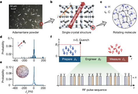
Figure 1: The experimental protocol. a, Microscopic picture of powder sample of adamantane (C₁₀H₁₆). The granules, whose sizes are of the order of micrometers, exhibit random orientations. b, In one granule, the adamantane molecules form a face-centered cubic lattice. The orientation of the static magnetic field $\mathbf{B}_{0}$ relative to the lattice principal axes determines the values of the secular dipolar coupling strength $J_{ij}$. c, Each molecule undergoes rapid rotation around its lattice site due to thermal motion, and the lattice site effectively serves as a time-averaged position for all the nuclear spins within the same molecule. ¹H carries nuclear spin-$1/2$ and ¹²C carries no spin. d,e, The probability distribution of the intermolecular coupling $J_{ij}$. d shows the distribution for a given orientation of $\mathbf{B}_{0}$, and e shows the distribution averaged over $10^{5}$ random orientations denoted by arrows in the spherical surface. Up to the 13th neighbor couplings are incorporated in the calculation code . f, The experimental protocol of the quench dynamics. Firstly we prepare a polarized initial density matrix $\hat{\rho}_{\alpha}\propto\mathbbm{1}+\epsilon\sum_{ia}\hat{S}_{ia}^{\alpha}$, $\alpha=\hat{x},\ \hat{y}$ or $\hat{z}$. Then, the state evolves under the anisotropic random spin models engineered by the RF pulse sequence illustrated below and also used in Refs. Suter1987 ; NMR_MBL2018 ; NMR_prethermal2019 ; NMR_Losch2020 ; NMR_prethermal2021 ; NMR_hydrodynamics2023 , after which we measure the magnetization $\hat{O}_{\alpha}=\sum_{ia}\hat{S}_{ia}^{\alpha}$.

To be concrete, let us consider an initial density matrix as $\hat{\rho}\propto\mathbbm{1}+\epsilon\hat{O}$, where $\epsilon$ is a small parameter and $\hat{O}$ is a traceless operator as a perturbation to the infinite temperature ensemble. This density matrix undergoes time evolution governed by a quantum many-body Hamiltonian $\hat{H}$, given by $\hat{\rho}(t)=\text{e}^{-\text{i}\hat{H}t/\hbar}\hat{\rho}~{}\text{e}^{\text{i}\hat{H}t/\hbar}$. Then, by measuring the expectation value of operator $\hat{O}$, we can access the auto-correlation function as $\langle\hat{O}(t)\rangle=\text{Tr}[\hat{O}\hat{\rho}(t)]\propto\mathcal{C}(t)$, where $\mathcal{C}(t)=\frac{1}{c_{O}}\text{Tr}[\hat{O}(t)\hat{O}(0)]$ is the auto-correlation function with normalization constant $c_{O}$ such that $\mathcal{C}(0)=1$. This auto-correlation function is defined at infinite temperatures because it equally incorporates contributions from all eigenstates, thereby reflecting the properties of the many-body Hamiltonian. During the Heisenberg evolution, the operator complexity of $\hat{O}(t)$ continuously increases complexity1 ; complexity2 , resulting in decaying of $\mathcal{C}(t)$. Therefore, the universality observed in $\mathcal{C}(t)$ ultimately stems from the universal behavior in the complexity theory of operator growth Zhai .

Our experiment is conducted on a powder sample of adamantane (C₁₀H₁₆) NMR_localization2015 ; NMR_Losch2020 ; Pastawski2009 ; Claudia2014 ; Suter2010 . Each adamantane molecule contains sixteen Hydrogen atoms (¹H), and each ¹H carries nuclear spin $S=1/2$. There are approximately $10^{9}$ to $10^{12}$ molecules contained in a single granule of the powder, which has a size on the order of micrometers (Fig. 1a). These spins interact with each other through magnetic dipolar interactions. Moreover, the sample is placed in a uniformed magnetic field of $B_{0}=9.4$ T along the $\hat{z}$ direction. Therefore, the Hamiltonian reads

$$\hat{H}=-\hbar\gamma_{\text{H}}B_{0}\sum\limits_{ia}\hat{S}^{z}_{ia}+$$

$$\sum\limits_{(i,a)<(j,b)}\frac{\mu_{0}\hbar^{2}\gamma^{2}_{\text{H}}}{4\pi r^{3}_{ia,jb}}\Bigg{[}\hat{\bm{S}}_{ia}\cdot\hat{\bm{S}}_{jb}-\frac{3(\hat{\bm{S}}_{ia}\cdot{\bf r}_{ia,jb})(\hat{\bm{S}}_{jb}\cdot{\bf r}_{ia,jb})}{r^{2}_{ia,jb}}\Bigg{]},$$ (1)

where $\hat{\bm{S}}_{ia}=(\hat{S}_{ia}^{x},\hat{S}_{ia}^{y},\hat{S}_{ia}^{z})$ are spin operators for each ¹H. $i$ and $j$ label molecules positioned on a face-centered cubic lattice (Fig. 1b). The indices $a,b=1,\dots,16$ label the spin-$1/2$ within each molecule. The constraint $(i,a)<(j,b)$ is defined as $a<b$ when $i=j$ and otherwise $i<j$. $\mu_{0}$ is the vacuum magnetic permeability and $\gamma_{\text{H}}$ is the proton’s gyromagnetic ratio. ${\bf r}_{ia,jb}={\bf R}_{ij}+{\bf l}_{a}-{\bf l}_{b}$ and $r_{ia,jb}=|{\bf r}_{ia,jb}|$, where ${\bf R}_{ij}$ denotes the displacement between centers of two molecules. ${\bf l}_{a}$ and ${\bf l}_{b}$ are the vectors from the center of the molecule to each nuclear spin carrier ¹H. $\gamma_{\text{H}}B_{0}$ represents the strength of the Zeeman splitting resulting from the external magnetic field.

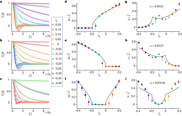
Figure 2: Dynamical evolution of spin polarization during the quench dynamics. a-c, Experimental measurements of $\mathcal{C}_{\alpha}(t)\propto\langle\hat{O}_{\alpha}\rangle$, with $\hat{O}_{\alpha}=\sum_{ia}\hat{S}_{ia}^{\alpha}$. The data is normalized by its value at $t=0$, with error bars ($\sim 10^{-4}$) incorporated within the markers of the data points. The initial state density matrix is prepared as $\hat{\rho}_{\alpha}\propto\mathbbm{1}+\epsilon\hat{O}_{\alpha}$, respectively. We have $\alpha=\hat{x}$ for (a), $\alpha=\hat{y}$ for (b), and $\alpha=\hat{z}$ for (c). Here we fix $\xi_{z}=0.2$ and $\sum_{\alpha}\xi_{\alpha}=0$ in the Hamiltonian Eq. (4). Different colors in the figures denote different values of $\xi_{x}$, varying from $-0.4$ to $0.2$. The solid lines represent the fittings using a general function $A\cos(\Omega t+\Phi)\exp(-\Lambda t)$, from which both $\Omega$ and $\Lambda$ are obtained. d-f, The oscillation frequencies $\Omega/\bar{J}$ extracted from (a-c) are plotted as a function of $\xi_{x}$ for $\alpha=\hat{x}$ (d), $\hat{y}$ (e) and $\hat{z}$ (f). The solid line denotes zero when $W_{\alpha}<0$ and fits $c\sqrt{W_{\alpha}}$ for $W_{\alpha}>0$. g-i, $\Lambda/\bar{J}$ extracted from (a-c) is plotted as a function of $\xi_{x}$ for $\alpha=\hat{x}$ (g), $\hat{y}$ (h) and $\hat{z}$ (i). The solid line fits $c\sqrt{\Gamma}$ when $W_{\alpha}>0$ and fits $c(\sqrt{\Gamma}-\sqrt{-W_{\alpha}})$ for $W_{\alpha}<0$. The constant $c$ is obtained from simultaneous fitting of both $\Omega/\bar{J}$ and $\Lambda/\bar{J}$, with the $95\%$ confidence interval in the parenthesis. The error bars of data points in (d-i) include both the $95\%$ confidence intervals estimated from the fitting residuals, and the fluctuation due to varying the fitting range (from $15$ to $41$ points) code . This strategy reduces the fitting error caused by the ambiguity of the fitting range, thereby enhancing the reliability of the fitting results.

At room temperature, each molecule undergoes rapid rotation around its center due to thermal motion, with a characteristic timescale of $10^{-11}$ s Resing1969 (Fig. 1c). This timescale is much faster than the timescale of dipolar interaction, which is approximately $10^{-3}$ s. By averaging the Hamiltonian over the solid angles of ${\bf l}_{a}$ and ${\bf l}_{b}$, and to the leading-order approximation, the Hamiltonian Eq. (1) becomes Resing1969 ; McCall1960 ; Smith1961

$$\hat{H}=\sum\limits_{i<j,ab} \frac{\mu_{0}\hbar^{2}\gamma^{2}_{\text{H}}}{4\pi R^{3}_{ij}}\left[\hat{\bm{S}}_{ia}\cdot\hat{\bm{S}}_{jb}-\frac{3(\hat{\bm{S}}_{ia}\cdot{\bf R}_{ij})(\hat{\bm{S}}_{jb}\cdot{\bf R}_{ij})}{R^{2}_{ij}}\right]$$

$$-\hbar\gamma_{\text{H}}B_{0}\sum\limits_{ia}\hat{S}^{z}_{ia}.$$ (2)

That is to say, a nuclear spin in one molecule interacts identically with any other nuclear spin in another molecule.

Furthermore, the presence of an external magnetic field causes all spins to rotate along the $\hat{z}$ direction, with a characteristic timescale of $10^{-9}$ s. This rapid motion can be effectively eliminated by applying a unitary transformation $\exp(-\text{i}\gamma_{\text{H}}B_{0}\sum\limits_{ia}\hat{S}^{z}_{ia}t)$. After taking the secular approximation Abragam1961 , we obtain the Hamiltonian

$$\hat{H}=\hbar\sum\limits_{i<j,ab}J_{ij}(-\hat{S}^{x}_{ia}\hat{S}^{x}_{jb}-\hat{S}^{y}_{ia}\hat{S}^{y}_{jb}+2\hat{S}^{z}_{ia}\hat{S}^{z}_{jb}),$$ (3)

where $J_{ij}\equiv(\mu_{0}/4\pi)(\hbar\gamma^{2}_{\text{H}}/2R^{3}_{ij})(1-3\cos^{2}\theta_{ij})$. $\theta_{ij}$ represents the angle between ${\bf R}_{ij}$ and the $\hat{z}$ direction. Now, the randomness arises because the molecules occupy lattice sites, and in a powder sample, the orientations between the lattice axes and the $\hat{z}$ direction are random. Fig. 1d-e present the probability distributions of $J_{ij}$ calculated from the lattice structure code , supporting the notion that $J_{ij}$ can be regarded as random variables, with a mean and variance satisfying $\overline{J_{ij}}=0$ and $\overline{J^{2}_{ij}}=4J^{2}/N$. $N=N_{\text{m}}N_{\text{a}}$ is the total number of spins, in which $N_{\text{m}}$ is the number of molecules and $N_{\text{a}}=16$ represents the number of ¹H in each molecule. We calibrate $J$ within the range of $2\pi[1432,1502]$ Hz supple , with an average value $\bar{J}=(2\pi)\ 1460$ Hz, which is used later in the notation of the dimensionless time scale $\bar{J}t$.

Next, by periodically applying a radio-frequency pulse sequence as shown in Fig. 1f Suter1987 ; NMR_MBL2018 ; NMR_prethermal2019 ; NMR_Losch2020 ; NMR_prethermal2021 ; NMR_hydrodynamics2023 , the Hamiltonian in Eq. (3) can be further engineered into a more general form according to the average Hamiltonian theory Haeberlen1968

$$\hat{H}=\hbar\sum\limits_{i<j,ab}J_{ij}(\xi_{x}\hat{S}^{x}_{ia}\hat{S}^{x}_{jb}+\xi_{y}\hat{S}^{y}_{ia}\hat{S}^{y}_{jb}+\xi_{z}\hat{S}^{z}_{ia}\hat{S}^{z}_{jb})+\dots$$ (4)

Here $\xi_{\alpha}$ ($\alpha=\hat{x},\ \hat{y},\ \hat{z}$) represents three anisotropic parameters that are subjected to a constraint $\sum_{\alpha}\xi_{\alpha}=0$, which is inherited from the Hamiltonian (3) and conserved under global rotations. Note that the measurement is summed over random crystalline orientations, which facilitates Eq. (4) a random spin model in the sense of ensemble average. The various configurations of $(\xi_{x},\ \xi_{y},\ \xi_{z})$ can be achieved by manipulating the pulse intervals (Methods and Supplementary Information supple ). The Floquet-engineered random spin model (4) is non-integrable and generically prethermalizes an initial state with finite energy to quasi equilibrium, which could be characterized by a canonical ensemble $\hat{\rho}_{\mathrm{pre}}=\mathrm{e}^{-\beta\hat{H}}/\mathcal{Z}$, with $\mathcal{Z}$ the partition function and $\beta$ determined by the initial-state energy Deutsch2018 ; Mori2016 ; Abanin2017 ; NMR_prethermal2019 ; NMR_prethermal2021 . The Hamiltonian information is thus inherited by the prethermal state $\hat{\rho}_{\mathrm{pre}}$, which can be learned via state tomography (Methods and Supplementary Information supple ). The deviations from the target Hamiltonian configurations are calibrated to be within $3\%$. The term $\dots$ in Eq. (4) represents residual terms other than $\hat{S}^{\alpha}_{ia}\hat{S}^{\alpha}_{jb}$, and the total weight of these terms has been calibrated to be less than $20\%$.

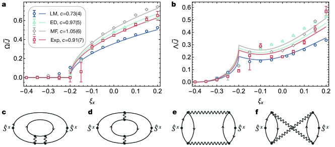
Figure 3: Theoretical results and diagrammatic analysis. a,b, We present the frequency (a) and decay rate (b) obtained respectively from the large-$M$ expansion (LM), exact diagonalization (ED), mean-field theory (MF), and the experimental data (Exp), which are represented by different colors code . The solid lines in (a),(b) are simultaneous fittings of the frequency $\Omega/\bar{J}$ and the decay rate $\Lambda/\bar{J}$ using their theoretical piecewise functions determined from Eq. (7): $(\Omega,\Lambda)/\bar{J}=c(\sqrt{W_{x}},\sqrt{\Gamma})$ when $W_{x}>0$, whereas $(\Omega,\Lambda)/\bar{J}=c(0,\sqrt{\Gamma}-\sqrt{-W_{x}})$ when $W_{x}<0$. The uncertainties of the constants $c$ in the parentheses denote the $95\%$ confidence intervals. c-f, These four diagrams represent contributions from (c) $\sum_{i,a}\operatorname{Tr}\left[\hat{H}^{2}\hat{S}_{ia}^{x}\hat{S}_{ia}^{x}\right]$, (d) $\sum_{i,a}\operatorname{Tr}\left[\hat{H}\hat{S}_{ia}^{x}\hat{H}\hat{S}_{ia}^{x}\right]$, (e) $\sum_{(i,a)\neq(j,b)}\operatorname{Tr}\left[\hat{H}\hat{S}_{ia}^{x}\hat{H}\hat{S}_{jb}^{x}\right]$ and (f) $\sum_{(i,a)\neq(j,b)}\operatorname{Tr}\left[\hat{H}^{2}\hat{S}_{ia}^{x}\hat{S}_{jb}^{x}\right]$. In each diagram, the dots represent spin operators, and two of them are labeled as $\hat{S}^{x}$ since they are the corresponding operators in the two-point correlator. The loops represent the trace of spin operators, while the arrows indicate the order of spin operator contractions. The wavy lines and their associated dots denote the vertices of random spin interactions.

In this experiment, we consider three different initial density matrices, denoted as $\hat{\rho}_{\alpha}\propto\mathbbm{1}+\epsilon\hat{O}_{\alpha}$. Here, $\hat{O}_{\alpha}=\sum_{ia}\hat{S}^{\alpha}_{ia}$ ($\alpha=\hat{x}$, $\hat{y}$, or $\hat{z}$) represents the total spin along different directions, and $\epsilon\approx 6.4\times 10^{-5}$. We evolve the initial density matrix under the Hamiltonian (4). Subsequently, we measure $\langle\hat{O}_{\alpha}(t)\rangle$. As discussed earlier, the result corresponds to the normalized auto-correlation function $\mathcal{C}_{\alpha}(t)$. The most remarkable finding of this experiment is the discovery of a universal functional form for $\mathcal{C}_{\alpha}(t)$. Specifically, for $\alpha=\hat{x}$, we introduce two quantities, namely, $W_{x}$ and $\Gamma$, which are quadratic polynomials of the microscopic parameters $\xi_{\alpha}$ proposed in Ref. Zhou :

$$W_{x}\equiv-\xi^{2}_{x}+\xi^{2}_{y}-4\xi_{y}\xi_{z}+\xi^{2}_{z},$$ (5)

$$\Gamma\equiv\xi^{2}_{x}+\xi^{2}_{y}+\xi^{2}_{z}.$$ (6)

Using these two polynomials, we can introduce two characteristic energy scales $\hbar\omega_{x}\equiv c\hbar\sqrt{|W_{x}|}J$ and $\hbar\lambda\equiv c\hbar\sqrt{\Gamma}J$. Here $c$ is an $o(1)$ constant. For $\alpha=\hat{y}$ or $\alpha=\hat{z}$, we can introduce $W_{y}$ and $W_{z}$ through permutation as $W_{y}=-\xi^{2}_{y}+\xi^{2}_{z}-4\xi_{z}\xi_{x}+\xi^{2}_{x}$ and $W_{z}=-\xi^{2}_{z}+\xi^{2}_{x}-4\xi_{x}\xi_{y}+\xi^{2}_{y}$. $\hbar\omega_{y}$ and $\hbar\omega_{z}$ are then defined correspondingly. We find that $\mathcal{C}_{\alpha}(t)$ can be well described by

$$\left\{\begin{aligned} &a\cos(\omega_{\alpha}t+\phi)\mathrm{e}^{-\lambda t},\ \ \text{if}\ \ W_{\alpha}>0,\\ &a\cosh(\omega_{\alpha}t+\phi)\mathrm{e}^{-\lambda t}\approx a^{\prime}\mathrm{e}^{-(\lambda-\omega_{\alpha})t}\ \ \text{if}\ \ W_{\alpha}<0,\end{aligned}\right.$$ (7)

where $a$, $a^{\prime}$ and $\phi$ are non-universal constants. This functional form is motivated by the quasinormal mode analysis for non-equilibrium dynamics. Quasinormal modes are collective modes with complex frequencies $\omega_{a}-i\lambda_{a}$, which govern the dynamically oscillatory and decaying response in strongly interacting systems normalmode1 ; normalmode2 . Here, $a$ labels different modes. In the long-time limit, we can retain only the mode with the smallest $\lambda_{a}$, resulting in the functional form proposed in Eq. (7) (see Methods and Supplementary Information supple for detailed derivation). Notably, our results firstly reveal the universal scaling functions between $(\omega_{\alpha},\lambda)$ and the microscopic parameters in the Hamiltonian, which has not been accomplished before to our best knowledge. As a consequence, this framework easily enables the establishment of a precise criterion for determining the presence of oscillatory or monotonic decay in spin relaxation dynamics. By offering a quantitative understanding, this advancement marks a significant step forward in alignment with prior research Fine2004 ; Fine2005 ; NMR_UniversalDecay2008 ; NMR_UniversalDecay2011 ; NMR_UniversalDecay2012 . Despite of the effectiveness and simplicity of Eq. (7), it is observed that it leads to larger deviations from the experimental data around the transition point $W_{\alpha}=0$, where the multi-mode dynamics become more significant.

Eq. (7) is demonstrated by the experimental data presented in Fig. 2. We polarize the system initially in three different directions $\alpha=\hat{x},\ \hat{y},\ \hat{z}$ respectively and then measure $\langle\hat{O}_{\alpha}\rangle$ for $\xi_{z}=0.2$ and $\xi_{x}\in[-0.4,0.2]$. The spin depolarization dynamics of $\langle\hat{O}_{\alpha}\rangle$ are depicted in Fig. 2a-c. We fit these curves using the function $A\cos(\Omega t+\Phi)e^{-\Lambda t}$ and obtain $\Omega$ and $\Lambda$ for each case. Importantly, this approach does not assume the existence of an oscillating-to-monotonic transition. Comparing to Eq. (7), we predict $(\Omega,\Lambda)=(\omega_{\alpha},\lambda)$ when $W_{\alpha}>0$, whereas $(\Omega,\Lambda)=(0,\lambda-\omega_{\alpha})$ when $W_{\alpha}<0$.

Given the constraint $\sum_{\alpha}\xi_{\alpha}=0$, we have $W_{x}=-6\xi_{y}\xi_{z}$, $W_{y}=-6\xi_{z}\xi_{x}$, and $W_{z}=-6\xi_{x}\xi_{y}$. In this experiment, we fix $\xi_{z}=0.2$. Thus, when $\alpha=\hat{x}$, we find $W_{x}=1.2(0.2+\xi_{x})>0$ for $\xi_{x}>-0.2$. As shown in Fig. 2a,d, the auto-correlation function oscillates when $\xi_{x}>-0.2$, and the frequency $\Omega/\bar{J}$ scales as $c\sqrt{W_{x}}$, where $\bar{J}$ is the average value of $J$ determined by experiment. Fig. 2g also demonstrates that $\Lambda/\bar{J}$ scales with $c\sqrt{\Gamma}$ for $\xi_{x}>-0.2$ and scales with $c(\sqrt{\Gamma}-\sqrt{-W_{x}})$ for $\xi_{x}<-0.2$. From the fitting, we obtain $c=0.91(7)$. Similarly, for $\alpha=\hat{y}$, we have $W_{y}=-1.2\xi_{x}>0$ for $\xi_{x}<0$, where the frequency $\Omega/\bar{J}$ fits $c\sqrt{W_{y}}$ and $\Lambda/\bar{J}$ fits $c\sqrt{\Gamma}$. For $\xi_{x}<0$, the frequency is zero, and $\Lambda/\bar{J}$ fits $c(\sqrt{\Gamma}-\sqrt{-W_{y}})$. The fittings result is $c=0.91(7)$, as shown in Fig. 2b,e,h. For $\alpha=\hat{z}$, $W_{z}=6\xi_{x}(0.2+\xi_{x})>0$ for $\xi_{x}>0$ or $\xi_{x}<-0.2$, where the frequency fits $c\sqrt{W_{z}}$ and $\Lambda/\bar{J}$ also fits $c\sqrt{\Gamma}$. For $-0.2<\xi_{x}<0$, the frequency is zero, and $\Lambda/\bar{J}$ fits $c(\sqrt{\Gamma}-\sqrt{-W_{z}})$. The fittings yield $c=0.87(10)$, as shown in Fig. 2c,f,i. The constants $c$ obtained from the three fittings are consistent with each other within the error bars.

As a self-consistent check, we note that when $\Gamma=-W_{x}$, $\Lambda=0$, and our ansatz shows that $\mathcal{C}_{x}(t)$ does not decay at all. It is easy to observe that $\Gamma=-W_{x}$ implies $\xi_{y}=\xi_{z}$, and the system restores spin rotational symmetry along $\hat{x}$. Therefore, $\hat{O}_{x}$ commutes with the Hamiltonian, and the total spin along $\hat{x}$ should not evolve in time. Similar conditions hold for $\alpha=\hat{y}$ or $\hat{z}$. This observation is also consistent with our experimental findings, indicating that our system remains coherent and the decoherence effect is negligible within the experimental timescale. Furthermore, these scaling behaviors have been confirmed by exact diagonalization calculations and approximation methods such as large-$M$ expansion and mean-field theory (see the Methods for further details) Zhou ; code . Each theoretical approach has its own advantages and disadvantages: The exact-diagonalization method captures the exact non-equilibrium quantum dynamics for $\operatorname{SU}(2)$ spin, but only with a small system size $N$. The semi-classical method captures the non-equilibrium spin dynamics through the Landau–Lifshitz equation of the non-equilibrium dynamics, with intermediate system size $N$. The large-$M$ expansion captures the leading order contribution to non-equilibrium dynamics in large system size $N$, which is rigorous at large-$M$ for $\operatorname{SU}(2)\times\operatorname{SU}(M)$ spin. It is remarkable that the same combinations of the anisotropic parameters in Hamiltonian enter the non-equilibrium dynamics, leading to the universal polynomial scaling on oscillation frequency and decay rate. In Fig. 3a,b, we compare $\Omega$ and $\Lambda$ obtained by these three theoretical methods with the experimental data and find good agreements. All the theory results also obey the universal function form shown in Eqs. (5)-(7), with a slightly different value $c$.

Below, we will discuss some physical intuitions as to why the quantities $W_{\alpha}$ and $\Gamma$ emerge as universal parameters in the quench dynamics. In low-energy physics, universality arises when a specific set of diagrams becomes the most relevant one and dominates the physical process under consideration, for instance, near a symmetry-breaking phase transition point in the Landau paradigm RMP . In our case, we argue that the same reasoning applies to the emergence of universality in the quench dynamics, albeit with a focus on the infinite temperature auto-correlation function $\mathcal{C}_{\alpha}(t)$.

Without loss of generality, we consider $\alpha=\hat{x}$ and the correlation function $\mathcal{C}_{x}(t)=\frac{1}{c_{O}}\sum_{ij,ab}\langle\hat{S}^{x}_{ia}(t)\hat{S}^{x}_{jb}(0)\rangle$. The experimental result suggests that dominant contributions to $\langle\hat{S}^{x}_{ia}(t)\hat{S}^{x}_{jb}(0)\rangle$ contain a few interaction channels, which can be identified by examining these terms $\langle\hat{H}\hat{S}^{x}_{ia}\hat{H}\hat{S}^{x}_{jb}\rangle$ and $\langle\hat{H}^{2}\hat{S}^{x}_{ia}\hat{S}^{x}_{jb}\rangle$ supple . This argument can be justified using the large-$M$ and mean-field theory Zhou , which are two of the most popular approximation schemes for studying spin models. The large-$M$ expansion has been particularly successful in studying a randomly interacting spin model known as the Sachdev-Ye (SY) model SY , which was later extended to the celebrated Sachdev-Ye-Kitaev model (SYK) SYK1 ; SYK2 ; SYK3 . These two terms can be illustrated by the Feynman diagrams shown in Fig. 3c-f, with contributions from $i=j$ given by Fig. 3c,d, and contributions from $i\neq j$ given by Fig. 3e,f. Lengthy but straightforward calculations demonstrate that the contribution from diagram Fig. 3c is exactly proportional to $\Gamma$ as defined in Eq. (6), while the contributions from diagrams Fig. 3d-f can be combined into $W_{x}$ as defined in Eq. (5) supple . The fact that the experimental data can be well captured by these parameters reveals the underlying physics behind the dynamics, indicating that this non-equilibrium process is dominated by the interaction processes shown in Fig. 3.

This universal behavior can also be applied to similar models realized in other physical systems. As a concrete example, a similar random spin model has been realized by Rydberg atoms excited in an ultracold atomic gas, and a non-monotonic dependence of the relaxation dynamics on the anisotropic parameter ratio has been observed Rydberg_Floquet2021 . This dependence also aligns with the dependency of the decay rate on the anisotropic parameters presented in this work.

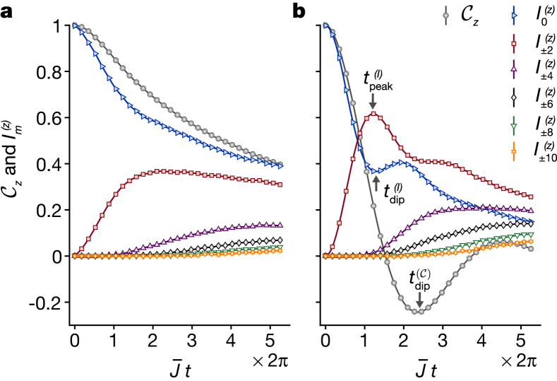
Figure 4: The multiple quantum coherences for randomly interacting spin models. MQC intensities of different order in the eigenbasis of $\hat{O}_{z}$, denoted as $I_{m}^{(z)}$, as a function of the evolution time $\bar{J}t$. The values of $(\xi_{x},\xi_{y},\xi_{z})$ are $(-0.125,-0.025,0.15)$ for a and $(-0.1,0.1,0)$ for b. At each time of $\bar{J}t$, the data is normalized by the value $F(\phi,t)|_{\phi=0}=\sum_{m}I_{m}^{(z)}(t)$, in order to ensure that $\sum_{m}I_{m}^{(z)}(t)=1$. The different curves represent various values of the coherence order $m$. The error bars ($\sim 10^{-4}$) are incorporated within the markers of the data points. The solid lines denote the cubic spline interpolations. In b, we extract that $I_{0}^{(z)}(t)$ reaches its initial trough at $\bar{J}t_{\mathrm{dip}}^{(I)}/2\pi\approx 1.29$, and $I_{\pm 2}^{(z)}(t)$ reaches its initial peak at $\bar{J}t_{\mathrm{peak}}^{(I)}/2\pi\approx 1.22$, while $\mathcal{C}_{z}(t)$ reaches its initial trough at $\bar{J}t_{\mathrm{dip}}^{(\mathcal{C})}/2\pi\approx 2.37$.

For a given direction $\alpha$, whether $W_{\alpha}>0$ or $W_{\alpha}<0$ not only distinguishes two types of quench dynamics for the two-point correlator but also marks the difference in higher-order correlators. We now investigate the higher-order correlation by studying the multiple quantum coherences (MQCs) Ernst1976 ; Ernst1977 ; Drobny1978 ; Bodenhausen1980 ; Pines1983 ; Pines1985 . The experimental protocol, such as described in Refs. Pines1983 ; Pines1985 , can be used to extract the MQC spectrum by utilizing its relation with the out-of-time-order (OTO) correlator $F(\phi,t)=\text{Tr}[\text{e}^{-\text{i}\hat{O}_{\alpha}\phi}\hat{O}_{\alpha}(t)\text{e}^{\text{i}\hat{O}_{\alpha}\phi}\hat{O}_{\alpha}(t)]$ NMR_OTOC2017 ; Ion_OTOC2017 ; Garttner2018 ; OTOC1 ; OTOC2 ; OTOC3 ; Maldacena2016 ; Hosur2016 ; Landsman2019 . $F(\phi,t)$ can be expanded as $F(\phi,t)=\sum_{m}I_{m}^{(\alpha)}(t)e^{-\text{i}m\phi}$, where $I_{m}^{(\alpha)}$ represents the intensity of the $m$th-order quantum coherences in the eigenbasis of $\hat{O}_{\alpha}$. $I_{0}^{(\alpha)}$ incorporates both the zero-quantum coherences and populations (diagonal elements).

In this protocol, we first evolve $\hat{\rho}_{\alpha}$ with the many-body Hamiltonian $\hat{H}$ for a time duration $t$. Then, we apply a spin rotation with angle $\phi$ given by $\exp(-\text{i}\hat{O}_{\alpha}\phi)$. This is followed by another evolution under the Hamiltonian $-\hat{H}$ for the same time duration $t$. Afterward, we measure the expectation value $\langle\hat{O}_{\alpha}\rangle$. Similar to the measurement of the auto-correlation function, this protocol allows us to measure the OTO correlator $F(\phi,t)$, since

$$\langle\hat{O}_{\alpha}\rangle =\text{Tr}[\text{e}^{\text{i}\hat{H}t/\hbar}\text{e}^{-\text{i}\hat{O}_{\alpha}\phi}\text{e}^{-\text{i}\hat{H}t/\hbar}\hat{\rho}_{\alpha}\text{e}^{\text{i}\hat{H}t/\hbar}\text{e}^{\text{i}\hat{O}_{\alpha}\phi}\text{e}^{-\text{i}\hat{H}t/\hbar}\hat{O}_{\alpha}]$$ (8)

$$=\text{Tr}[\text{e}^{-\text{i}\hat{O}_{\alpha}\phi}\hat{\rho}_{\alpha}(t)\text{e}^{\text{i}\hat{O}_{\alpha}\phi}\hat{O}_{\alpha}(t)]\propto F(\phi,t).$$

Then, by varying the rotation angle $\phi$ and time duration $t$, and subsequently applying a Fourier transform with respect to $\phi$, the MQC spectrum $\{I_{m}^{(\alpha)}(t)\}$ can be obtained. It is worth noting that $\partial^{2}F(\phi,t)/\partial\phi^{2}|_{\phi=0}=-\sum_{m}I_{m}^{(\alpha)}(t)m^{2}=\operatorname{Tr}([\hat{O}_{\alpha}(t),\hat{O}_{\alpha}]^{2})$, which is the OTO commutator Garttner2018 . This connection between MQC and OTO commutator allows us to characterize information scrambling in the system Garttner2018 .

In Fig. 4, we present the results of $I_{m}^{(\alpha)}(t)$ for two cases with $\alpha=\hat{z}$. Fig. 4a depicts the case with $(\xi_{x},\xi_{y},\xi_{z})=(-0.125,-0.025,0.15)$, where $W_{z}=-0.01875<0$. In this scenario, we observe a monotonic decay of $I_{0}^{(z)}$, with its weight gradually spreading into higher-order quantum coherences. Fig. 4b illustrates the case with $(\xi_{x},\xi_{y},\xi_{z})=(-0.1,0.1,0)$ and $W_{z}=0.06>0$. In this situation, clear oscillations are observed in both $I_{0}^{(z)}(t)$ and $I_{\pm 2}^{(z)}(t)$. Besides, it seems that $I_{0}^{(z)}(t)$ and $I_{\pm 2}^{(z)}(t)$ oscillate with a frequency roughly double that of $\mathcal{C}_{z}(t)$, as indicated by the time points when $I_{0}^{(z)}(t)$, $I_{\pm 2}^{(z)}(t)$ and $\mathcal{C}_{z}(t)$ reach their initial trough or peak: $\bar{J}t_{\mathrm{dip}}^{(I)}/2\pi\approx 1.29$, $\bar{J}t_{\mathrm{peak}}^{(I)}/2\pi\approx 1.22$, and $\bar{J}t_{\mathrm{dip}}^{(\mathcal{C})}/2\pi\approx 2.37$. This is reasonable considering that the OTO commutator $\operatorname{Tr}([\hat{O}_{z}(t),\hat{O}_{z}]^{2})$ involves a square of $\hat{O}_{z}(t)\hat{O}_{z}$. This observation is further verified by varying the Hamiltonian configurations (see Supplementary Information supple ).

To conclude, we experimentally study the far-from-equilibrium quench dynamics in randomly interacting spin models using solid-state NMR systems. The mean strength of random interaction is the only energy scale in the Hamiltonian governing the dynamics. Hence, this problem is intrinsically a strongly interacting many-body problem that lacks small perturbation parameters, and such a system at non-equilibrium belongs to the most challenging problems for developing physical understandings. The numerical method, like exact diagonalization, is limited to a system size much smaller than the actual physical system and does not provide insightful physical intuitions. The approximation scheme, such as large-M theory, does provide helpful intuition but involves uncontrolled errors. In light of these challenges, quantitative comparison between theory and experiment becomes particularly valuable. To this end, accurate calibration of Hamiltonian parameters and high-quality data on quantum dynamics with insignificant decoherence effects are required. Here, by reaching a consistency between experiment, approximated theory, and numerical diagonalization, we reveal a few universal parameters and uncover dominating interacting processes for this quench dynamics, which can be generalized to similar non-equilibrium dynamics in cold atoms, NV centers, and other systems.

Methods

Hamiltonian Engineering. By periodically applying the radio-frequency (RF) pulse sequence to the natural dipolar Hamiltonian, we can engineer the desired form of the anisotropic Heisenberg models (4) as an effective time-independent Hamiltonian by the average Hamiltonian theory Haeberlen1968 . The basic building block of the RF pulse train is an 8-pulse sequence initially introduced for studying multiple quantum coherences Suter1987 . Explicitly, the 8-pulse sequence is represented as follows:

$$(\tau_{z},\mathbf{x},\tau_{y},\mathbf{y},2\tau_{x},\mathbf{y},\tau_{y},\mathbf{x},2\tau_{z},\mathbf{x},\tau_{y},\mathbf{y},2\tau_{x},\mathbf{y},\tau_{y},\mathbf{x},\tau_{z}),$$

where $\mathbf{x}$ and $\mathbf{y}$ denote the RF pulses that induce collective $\pi/2$ rotations along the $\hat{x}$ and $\hat{y}$ directions, respectively. By adjusting the pulse intervals $\tau_{\alpha}$ such that $\tau_{\alpha}=\left[1+\xi_{\alpha}\right]\tau$, we can realize different configurations of the anisotropic parameters $(\xi_{x},\ \xi_{y},\ \xi_{z})$ to the leading order of the Magnus expansion Magnus1954 ; supple .

Hamiltonian Calibration. We calibrate the actually realized anisotropic parameters $(\xi_{x}^{\prime},\ \xi_{y}^{\prime},\ \xi_{z}^{\prime})$ and the weight of residual terms other than $\hat{S}^{\alpha}_{ia}\hat{S}^{\alpha}_{jb}$ in the effective Floquet Hamiltonian $\hat{H}_{\mathrm{F}}$. The idea is to employ Floquet prethermalization hypothesis Mori2016 ; Abanin2017 . It assumes that the system attains a quasi-stationary state $\hat{\rho}_{\mathrm{pre}}$, approximately characterized by a canonical ensemble associated with the effective Hamiltonian $\hat{H}_{\mathrm{F}}$, before heated to the infinite temperature. We have

$$\hat{\rho}_{\mathrm{pre}}\approx\frac{e^{-\beta_{\text{eff}}\hat{H}_{\mathrm{F}}}}{\operatorname{Tr}\small(e^{-\beta_{\text{eff}}\hat{H}_{\mathrm{F}}}\small)}\propto\mathbbm{1}-\beta_{\text{eff}}\hat{H}_{\mathrm{F}},$$ (9)

where $\beta_{\text{eff}}$ represents an effective inverse temperature, determined by the initial state $\hat{\rho}_{0}$ through the energy conservation $\operatorname{Tr}(\hat{\rho}_{0}\hat{H}_{\text{F}})=\operatorname{Tr}(\hat{\rho}_{\text{pre}}\hat{H}_{\text{F}})$. The Floquet prethermalization has been experimentally demonstrated in spin chains with dipolar interactions NMR_prethermal2019 ; NMR_prethermal2021 .

As elaborated in the Supplementary Information supple , we initially prepare states with finite inverse spin temperatures, and then allow them to prethermalize under the $\hat{H}$ Eq. (4) with various anisotropic configurations for a time period of $\bar{J}t\geq 14\pi$. In addition, we prepare dipolar-ordered states Jeener1967 ; Cho2003 as a reference state using the Jeener-Broekaert method Jeener1967 . The traceless components of the density matrix of these states are given by

$$\delta\hat{\rho}_{x}^{\mathcal{D}} \propto\sum\limits_{i\neq j,ab}J_{ij}(-\hat{S}^{y}_{ia}\hat{S}^{y}_{jb}-\hat{S}^{z}_{ia}\hat{S}^{z}_{jb}+2\hat{S}^{x}_{ia}\hat{S}^{x}_{jb}),$$ (10)

and the other two dipolar-ordered states $\delta\hat{\rho}_{y}^{\mathcal{D}},\ \delta\hat{\rho}_{z}^{\mathcal{D}}$ can be determined through cyclic permutations. In experiment, we measure the inner products between the prethermal state and each of the dipolar-ordered states. These inner products are proportional to the anisotropic parameters

$$\operatorname{Tr}\left(\hat{\rho}_{\mathrm{pre}}\delta\hat{\rho}_{x}^{\mathcal{D}}\right)\propto(2\xi_{x}^{\prime}-\xi_{y}^{\prime}-\xi_{z}^{\prime})\sum\limits_{i\neq j,ab}J_{ij}^{2}\propto\xi_{x}^{\prime}.$$ (11)

Similarly, we find $\operatorname{Tr}\small(\hat{\rho}_{\mathrm{pre}}\delta\hat{\rho}_{y}^{\mathcal{D}}\small)\propto\xi_{y}^{\prime}$ and $\operatorname{Tr}\small(\hat{\rho}_{\mathrm{pre}}\delta\hat{\rho}_{z}^{\mathcal{D}}\small)\propto\xi_{z}^{\prime}$. This determines the actual anisotropic parameters $(\xi_{x}^{\prime},\ \xi_{y}^{\prime},\ \xi_{z}^{\prime})$. The discrepancies between these parameters and their target values $(\xi_{x},\ \xi_{y},\ \xi_{z})$ are quantified by $\Delta\equiv\left|\bm{\xi^{\prime}}-\bm{\xi}\right|/\left|\bm{\xi}\right|$. Throughout all the realized configurations, the values of $\Delta$ are calibrated to be within $3\%$ supple .

The weight of residual terms denoted as $\cdots$ in the overall effective Hamiltonian Eq. (4) is defined by $\varepsilon\equiv\sqrt{\operatorname{Tr}\small(\cdots^{2}\small)/\operatorname{Tr}\small(\hat{H}^{2}\small)}$. It primarily leverages the orthogonal relationships between the residual term in the prethermal states $\hat{\rho}_{\mathrm{pre}}$ and the dipolar-ordered states $\delta\hat{\rho}^{\mathcal{D}}_{\alpha}$, and incorporates more inner product measurements. The values of $\varepsilon$ are determined to be less than $20\%$ across all the realized configurations supple .

Exact Diagonalization. In the exact diagonalization calculation, we are restricted to a simplified model consisting of a single spin-1/2 on each molecule with system size up to $N=8$. The Hamiltonian is

$$\hat{H}_{\text{ED}}=\sum\limits_{i<j}J_{ij}(\xi_{x}\hat{S}^{x}_{i}\hat{S}^{x}_{j}+\xi_{y}\hat{S}^{y}_{i}\hat{S}^{y}_{j}+\xi_{z}\hat{S}^{z}_{i}\hat{S}^{z}_{j}),$$ (12)

where $J_{ij}$ is modelled as a random variable obeying a normal distribution $J_{ij}\sim\mathcal{N}[0,(2J/\sqrt{N})^{2}]$. For each disorder realization of $J_{ij}$, we prepare the initial state as a thermal density matrix, denoted as $\hat{\rho}\propto\exp(-\beta(\hat{H}_{\text{ED}}+\hat{\delta H}))$, where $\beta=\hbar/(k_{B}T)$ denotes the inverse temperature and an external polarization field is introduced as $\hat{\delta H}=-g\sum_{i}\hat{S}^{x}_{i}$. We fix $\beta J=0.2$ and $g/J=2$, as explained later in Parameters in Numerical Simulations. The system is then evolved under the Hamiltonian Eq. (12), and the result is averaged over $10^{3}$ random realizations.

Large-$M$ Expansion. We can transform the randomly interacting spin model Eq. (4) into a theory of randomly interacting fermions by adopting the Abrikosov fermion representation. In this representation, the spin operators are expressed as $\hat{S}^{\alpha}_{ia}=\frac{1}{2}\sum_{ss^{\prime}}\hat{c}^{\dagger}_{ia,s}(\sigma^{\alpha})_{ss^{\prime}}\hat{c}_{ia,s^{\prime}}$ ($s,s^{\prime}=\uparrow,\downarrow$), limited to the single occupation subspace. Our main interest lies in the spin polarization dynamics, which can be expressed as $\langle\hat{O}_{x}(t)\rangle=-iN(G^{\gtrless}_{\uparrow\downarrow}(t,t)+G^{\gtrless}_{\downarrow\uparrow}(t,t))/2$. Here the real-time Green’s functions are defined as $G^{>}_{ss^{\prime}}(t_{1},t_{2})\equiv-i\langle c_{ia,s}(t_{1})c_{ia,s^{\prime}}^{\dagger}(t_{2})\rangle$ and $G^{<}_{ss^{\prime}}(t_{1},t_{2})\equiv i\langle c_{ia,s^{\prime}}^{\dagger}(t_{2})c_{ia,s}(t_{1})\rangle$. The evolution of these Green’s functions can be described by a set of classical equations, commonly known as the Kadanoff-Baym equation

$$i\partial_{t_{1}} G^{\gtrless}=\Sigma^{R}\circ G^{\gtrless}+\Sigma^{\gtrless}\circ G^{A},$$ (13)

$$-i\partial_{t_{2}} G^{\gtrless}=G^{R}\circ\Sigma^{\gtrless}+G^{\gtrless}\circ\Sigma^{A},$$

where $G^{R/A}$ is the retarded/advanced Green’s function. $\Sigma^{\gtrless}$ and $\Sigma^{R/A}$ represent real-time self-energies, which satisfy $\Sigma^{R/A}=\pm\Theta\left(\pm t_{12}\right)\left(\Sigma^{>}-\Sigma^{<}\right)$. To make further theoretical advancements, an SU(M)$\times$SU(2) generalization has been introduced, similar to the approach used in large-M ; Zhou . By taking both the large-$N$ and the large-$M$ limit, melon diagrams play a dominant role in the self-energies, similar as in the SYK model. This leads to

$$\Sigma^{\gtrless}(t_{1},t_{2})=\frac{J^{2}}{4} \sum_{\alpha,\alpha^{\prime}}\xi_{\alpha}\xi_{\alpha^{\prime}}\sigma^{\alpha^{\prime}}G^{\gtrless}(t_{1},t_{2})\sigma^{\alpha}$$ (14)

$$\text{Tr}\left[\sigma^{\alpha^{\prime}}G^{\gtrless}(t_{1},t_{2})\sigma^{\alpha}G^{\lessgtr}(t_{2},t_{1})\right].$$

Numerically, we prepare the system in an initial state described by a thermal ensemble at $\beta J=0.2$ with a polarization field $g/J=2$. The corresponding initial Green’s functions are obtained through iterations. Subsequently, we evolve $G^{\gtrless}$ by combining Eq. (13) and Eq. (14) to determine $\langle\hat{O}_{x}(t)\rangle$. Besides, by conducting a quasinormal mode analysis, one can analytically derive the long-time spin relaxation dynamics Eq. (7) within the large-$M$ approximation Zhou . This calculation is elaborated in the Supplementary Information supple .

Mean-field Theory. Another theoretical scheme for analyzing randomly interacting spin models is the mean-field theory. Here, we introduce the average polarization on each molecule as $\hat{M}_{i}^{\alpha}=\frac{1}{N_{a}}\sum_{a}\hat{S}_{ia}^{\alpha}$. Due to the statistical averaging, we expect the fluctuation of $\hat{M}_{i}^{\alpha}$ to be small, allowing us to approximate it as a classical vector $M_{i}^{\alpha}$. The Heisenberg equation for $\hat{M}$ then becomes:

$$\frac{dM_{i}^{\alpha}}{dt}=N_{a}\sum_{j,\beta\gamma}J_{ij}\epsilon^{\alpha\beta\gamma}\xi_{\beta}M_{j}^{\beta}M_{i}^{\gamma}.$$ (15)

In the numerical simulation, we investigate a system with $2\times 10^{3}$ molecules. The initial configuration of $M_{i}^{\alpha}$ is randomly generated using an independent Gaussian distribution, with mean value $\overline{\bm{M}_{i}}=(\frac{\beta g}{4},0,0)$, $\beta g=0.4$ and variance $\overline{(\delta M_{i}^{\alpha})^{2}}=1/(4N_{a})$. Subsequently, we evolve $M_{i}^{\alpha}$ according to Eq. (15) for each random realization and compute $\langle\hat{O}^{\alpha}\rangle=N_{a}\sum_{i}M_{i}^{\alpha}$. The final result is then averaged over 20 independent simulations.

Parameters in Numerical Simulations. The NMR experiment is conducted at room temperature, necessitating the conditions $\beta J\ll 1$ and $\beta g\ll 1$. Additionally, the external magnetic field strongly polarizes the state, allowing the initial state to be approximated by $\hat{\rho}\propto\mathrm{e}^{-\beta\hat{H}_{\mathrm{dip}}+\beta g\sum_{ia}\hat{S}_{ia}^{\alpha}}\approx\hat{\mathbbm{1}}+\beta g\sum_{ia}\hat{S}_{ia}^{\alpha}$. This requires that the magnitude of the external field must be significantly larger than the characteristic strength of the dipolar interaction $\hat{H}_{\mathrm{dip}}$ [see Eq. (3)], i.e., $g/J\gg 1$. For numerical simulations, all parameters satisfy these conditions. In the Supplementary Information supple , we demonstrate that a moderate change of parameters yield qualitatively similar results. In particular, the oscillation frequencies and decay rates remain independent of $\beta$ and $g$ supple .

References

- (1) Chin, C., Grimm, R., Julienne, P., and Tiesinga, E. Feshbach resonances in ultracold gases. Rev. Mod. Phys. 62, 1225 (2010).
- (2) Pethick, C. J., and Smith, H. Bose–Einstein Condensation in Dilute Gases (Cambridge University Press, 2008).
- (3) Sachdev, S. Quantum Phase Transitions (Cambridge University Press, 2011).
- (4) Wei, D. et al. Quantum gas microscopy of Kardar-Parisi-Zhang superdiffusion. Science 376, 716-720 (2022).
- (5) Geier, S. et al. Floquet Hamiltonian engineering of an isolated many-body spin system. Science 374, 1149 (2021).
- (6) Gärttner, M. et al. Measuring out-of-time-order correlations and multiple quantum spectra in a trapped-ion quantum magnet. Nat. Phys. 13, 781–786 (2017).
- (7) Joshi, M. K. et al. Observing emergent hydrodynamics in a long-range quantum magnet. Science 376, 720–724 (2022).
- (8) Zu, C. et al. Emergent hydrodynamics in a strongly interacting dipolar spin ensemble. Nature 597, 45–50 (2021).
- (9) L. S. Martin et al. Controlling Local Thermalization Dynamics in a Floquet-Engineered Dipolar Ensemble. Phys. Rev. Lett. 130, 210403 (2023).
- (10) Morgan, S. W., Fine, B. V. and Saam, B. Universal Long-Time Behavior of Nuclear Spin Decays in a Solid. Phys. Rev. Lett. 101, 067601 (2008).
- (11) Sorte, E. G., Fine, B. V. and Saam, B. Long-time behavior of nuclear spin decays in various lattices. Phys. Rev. B 83, 064302 (2011).
- (12) Meier, B., Kohlrautz, J. and Haase, J. Eigenmodes in the Long-Time Behavior of a Coupled Spin System Measured with Nuclear Magnetic Resonance. Phys. Rev. Lett. 108, 177602 (2012).
- (13) Álvarez, G. A., Suter, D. and Kaiser, R. Localization-delocalization transition in the dynamics of dipolar-coupled nuclear spins. Science 349, 846–848 (2015).
- (14) Rovny, J., Blum, R. L. and Barrett, S. E. Observation of Discrete-Time-Crystal Signatures in an Ordered Dipolar Many-Body System. Phys. Rev. Lett. 120, 180603 (2018).
- (15) Wei, K. X., Ramanathan, C. and Cappellaro, P. Exploring Localization in Nuclear Spin Chains. Phys. Rev. Lett. 120, 070501 (2018).
- (16) Ramanathan, C., Cappellaro, P., Viola, L. and Cory, D. G. Experimental characterization of coherent magnetization transport in a one-dimensional spin system. New J. Phys. 13, 103015 (2011).
- (17) Li, J. et al. Measuring out-of-time-order correlators on a nuclear magnetic resonance quantum simulator. Phys. Rev. X 7, 031011 (2017).
- (18) Wei, K. X. et al. Emergent Prethermalization Signatures in Out-of-Time Ordered Correlations. Phys. Rev. Lett. 123, 090605 (2019).
- (19) Sánchez, C. M. et al. Perturbation Independent Decay of the Loschmidt Echo in a Many-Body System. Phys. Rev. Lett. 124, 030601 (2020).
- (20) Peng, P., Yin, C., Huang, X., Ramanathan, C. and Cappellaro, P. Floquet prethermalization in dipolar spin chains. Nat. Phys. 17, 444–447 (2021).
- (21) Peng, P., Ye, B., Yao, N. Y. and Cappellaro, P. Exploiting disorder to probe spin and energy hydrodynamics. Nat. Phys. 19, 1027–1032 (2023).
- (22) Fine, B. V. Long-time relaxation on spin lattice as a manifestation of chaotic dynamics. Int. J. Mod. Phys. B 18, 1119–1159 (2004).
- (23) Fine, B. V. Long-Time Behavior of Spin Echo. Phys. Rev. Lett. 94, 247601 (2005).
- (24) Ljubotina, M., Žnidarič, M. and Prosen, T. Spin diffusion from an inhomogeneous quench in an integrable system. Nat. Commun. 8, 16117 (2017).
- (25) Ljubotina, M., Žnidarič, M. and Prosen, T. Kardar-Parisi-Zhang physics in the quantum Heisenberg magnet. Phys. Rev. Lett. 122, 210602 (2019).
- (26) Gopalakrishnan, S. and Vasseur, R. Kinetic theory of spin diffusion and superdiffusion in XXZ spin chains. Phys. Rev. Lett. 122, 127202 (2019).
- (27) Gopalakrishnan, S., Vasseur, R. and Ware, B. Anomalous relaxation and the high-temperature structure factor of XXZ spin chains. Proc. Natl. Acad. Sci. U.S.A. 116, 16250–16255 (2019).
- (28) Dupont, M. and Moore, J. E. Universal spin dynamics in infinite-temperature one-dimensional quantum magnets. Phys. Rev. B 101, 121106 (2020).
- (29) Ljubotina, M., Desaules, J.-Y., Serbyn, M. and Papić, Z. Superdiffusive energy transport in kinetically constrained models. Phys. Rev. X 13, 011033 (2023).
- (30) Zhang, R. and Zhai, H. Universal Hypothesis of Autocorrelation Function from Krylov Complexity. Preprint at https://doi.org/10.48550/arXiv.2305.02356.
- (31) The data and code for Fig. 3 is available at https://github.com/tgzhou98/Quench-Random-Spin, which contains three packages of numerical simulations, and one package for fitting and corresponding error bar analysis. The data and code involved in Figs. 1,2,4 and the Supplementary Information supple are available at https://github.com/lyuchen96/Quench-Random-Spin, of which one package is for calculating the distribution of .
- (32) Suter, D., Liu, S. B., Baum, J. and Pines, A. Multiple quantum NMR excitation with a one-quantum hamiltonian. Chem. Phys. 114, 103–109 (1987).
- (33) Roberts, D. A., Stanford, D. and Susskind, L. Localized shocks. J. High Energ. Phys. 2015, 51 (2015).
- (34) Parker, D. E., Cao, X., Avdoshkin, A., Scaffidi, T. and Altman, E. A universal operator growth hypothesis. Phys. Rev. X 9, 041017 (2019).
- (35) Rufeil-Fiori, E., Sánchez, C. M., Oliva, F. Y., Pastawski, H. M. and Levstein, P. R. Effective one-body dynamics in multiple-quantum NMR experiments. Phys. Rev. A 79, 032324 (2009).
- (36) Sánchez, C. M., Acosta, R. H., Levstein, P. R., Pastawski, H. M., and Chattah, A. K. Clustering and decoherence of correlated spins under double quantum dynamics. Phys. Rev. A 90, 042122 (2014).
- (37) Álvarez, G. A. and Suter, D. NMR Quantum Simulation of Localization Effects Induced by Decoherence. Phys. Rev. Lett. 104, 230403 (2010).
- (38) H. A. Resing. NMR relaxation in adamantane and hexamethylenetetramine: Diffusion and rotation. Mol. Cryst. Liq. Cryst. 9, 101–132 (1969).
- (39) McCall, D. W. and Douglass, D. C. Nuclear magnetic resonance in solid adamantane. J. Chem. Phys. 33, 777–778 (1960).
- (40) Smith, G. W. On the Calculation of Second Moments of Nuclear Magnetic Resonance Lines for Large Molecules. Adamantane Molecule. J. Chem. Phys. 35, 1134–1135 (1961).
- (41) Abragam, A. The Principles of Nuclear Magnetism (Oxford University Press, 1961).
- (42) See supplementary information for (1) Experimental system; (2) Hamiltonian engineering; (3) Hamiltonian calibration; (4) Comparison between dynamics of the global auto-correlation function and the multiple quantum coherences; (5) Theoretical analysis.
- (43) Haeberlen, U. and Waugh, J. S. Coherent averaging effects in magnetic resonance. Phys. Rev. 175, 453 (1968).
- (44) Deutsch, J. M. Eigenstate thermalization hypothesis. Rep. Prog. Phys. 81, 082001 (2018).
- (45) Mori, T., Kuwahara, T. and Saito, K. Rigorous Bound on Energy Absorption and Generic Relaxation in Periodically Driven Quantum Systems. Phys. Rev. Lett. 116, 120401 (2016).
- (46) Abanin, D. A., De Roeck, W., Ho, W. W. and Huveneers, F. Effective Hamiltonians, prethermalization, and slow energy absorption in periodically driven many-body systems. Phys. Rev. B 95, 014112 (2017).
- (47) Konoplya, R. A. and Zhidenko, A. Quasinormal modes of black holes: From astrophysics to string theory. Rev. Mod. Phys. 83, 793–836 (2011).
- (48) Witczak-Krempa, W. and Sachdev, S. Quasinormal modes of quantum criticality. Phys. Rev. B 86, 235115 (2012).
- (49) Zhou, T. G., Zheng, W. and Zhang, P. Universal Aspect of Relaxation Dynamics in Random Spin Models. Preprint at https://doi.org/10.48550/arXiv.2305.02359.
- (50) Shankar, R. Renormalization-group approach to interacting fermions. Rev. Mod. Phys. 66, 129 (1994).
- (51) Sachdev, S. and Ye, J. Gapless spin-fluid ground state in a random quantum Heisenberg magnet. Phys. Rev. Lett. 70, 3339 (1993).
- (52) Kitaev, A. A simple model of quantum holography (part 2). Talk at KITP. Univ. California Santa Barbara https://online.kitp.ucsb.edu/online/entangled15/kitaev2/ (2015).
- (53) Maldacena, J. and Stanford, D. Remarks on the Sachdev-Ye-Kitaev model. Phys. Rev. D 94, 106002 (2016).
- (54) Chowdhury, D., Georges, A., Parcollet, O. and Sachdev, S. Sachdev-Ye-Kitaev models and beyond: Window into non-Fermi liquids. Rev. Mod. Phys. 94, 035004 (2022).
- (55) Altland, A., and Simons, B. D. Condensed matter field theory (Cambridge university press, 2010).
- (56) Aue, W. P., Bartholdi, E. and Ernst, R. R. Two‐dimensional spectroscopy. Application to nuclear magnetic resonance. J. Chem. Phys. 64, 2229–2246 (1976).
- (57) Wokaun, A. and Ernst, R. R. Selective detection of multiple quantum transitions in NMR by two-dimensional spectroscopy. Chem. Phys. Lett. 52, 407–412 (1977).
- (58) Drobny, G., Pines, A., Sinton, S., Weitekamp, D. P. and Wemmer, D. Fourier transform multiple quantum nuclear magnetic resonance. Faraday Symp. Chem. Soc. 13, 49 (1978).
- (59) Bodenhausen, G. Multiple-quantum NMR. Prog Nucl Magn Reson Spectrosc 14, 137–173 (1980).
- (60) Yen, Y. and Pines, A. Multiple‐quantum NMR in solids. J. Chem. Phys. 78, 3579–3582 (1983).
- (61) Baum, J., Munowitz, M., Garroway, A. N. and Pines, A. Multiple‐quantum dynamics in solid state NMR. J. Chem. Phys. 83, 2015–2025 (1985).
- (62) Gärttner, M., Hauke, P. and Rey, A. M. Relating out-of-time-order correlations to entanglement via multiple-quantum coherences. Phys. Rev. Lett. 120, 040402 (2018).
- (63) Larkin, A. I. and Ovchinnikov, Y. N. Quasiclassical method in the theory of superconductivity. Sov. phys. JETP 28, 1200–1205 (1969).
- (64) Shenker, S. H. and Stanford, D. Multiple shocks. J. High Energy Phys. 2014, 46 (2014).
- (65) Kitaev, A. Hidden correlations in the Hawking radiation and thermal noise. Talk given at the Fundamental Physics Prize Symposium (2014).
- (66) Hosur, P., Qi, X.-L., Roberts, D. A. and Yoshida, B. Chaos in quantum channels. J. High Energy Phys. 2016, 4 (2016).
- (67) Maldacena, J., Shenker, S. H. and Stanford, D. A bound on chaos. J. High Energy Phys. 2016, 106 (2016).
- (68) Landsman, K. A. et al. Verified quantum information scrambling. Nature 567, 61 (2019).
- (69) Magnus, W. On the exponential solution of differential equations for a linear operator. Commun Pure Appl Math 7, 649–673 (1954).
- (70) Jeener, J. and Broekaert, P. Nuclear Magnetic Resonance in Solids: Thermodynamic Effects of a Pair of rf Pulses. Phys. Rev. 157, 232–240 (1967).
- (71) Cho, H., Cory, D. G. and Ramanathan, C. Spin counting experiments in the dipolar-ordered state. J. Chem. Phys. 118, 3686–3691 (2003).
- (72) Zhou, T. G., Pan, L., Chen, Y., Zhang, P. and Zhai, H. Disconnecting a traversable wormhole: Universal quench dynamics in random spin models. Phys. rev. res. 3, L022024 (2021).