Stellar-Mass Black Holes with Dark Matter Mini-Spikes:
Evidence of a Primordial Origin?
Abstract
Recent observations of three nearby black hole low-mass X-ray binaries have suggested possible evidence of dark matter density spikes. It has long been established that cold dark matter should form dense spikes around intermediate-mass and supermassive black holes due to adiabatic compression of the surrounding dark matter halo. Lighter black holes formed from stellar collapse, however, are not expected to develop such spikes, and so it is unclear how the stellar-mass black holes in these binaries could have acquired such features. Given that primordial black holes are expected to form ultra-dense dark matter mini-spikes, in this Letter we explore the possibility that these stellar-mass black holes may actually have a primordial origin.
I Introduction
Observations of three nearby black hole low-mass X-ray binaries (BH-LMXBs) have revealed anomalously fast orbital decay rates for the companion star. The BH-LMXBs A0620-00, XTE J1118+480, and Nova Muscae 1991 each consist of an black hole and a much lighter () companion star with nearly circular orbit and short orbital period [1, 2, 3, 4, 5, 6, 7]. For such systems, the dominant sources of angular momentum loss are magnetic braking [8], mass transfer from the donor star [9], and gravitational wave emission, from which we expect [7]. These mechanisms appear wholly inadequate to account for the measured decay rates: for A0620-00, for XTE J1118+480, and for Nova Muscae 1991 [3, 10, 7].
An extremely strong stellar magnetic field could in principle account for the decay of A0620-00, though this is inconsistent with the observed binary mass loss rate [3]. Other potential explanations have invoked angular momentum loss due to interactions between the circumbinary disk and the inner binary [11]. However the inferred mass transfer rate and circumbinary disk mass appear insufficient for this hypothesis to be viable [12]. At present, the origin of these rapid decays remains a mystery which challenges the current paradigm of BH-LMXB evolution and whose resolution likely requires the introduction of some as-yet-unknown element.
The authors of Ref. [13] recently put forth the possibility that dynamical friction due to a dark matter (DM) density spike about the BH may be responsible for the rapid orbital decays in these binaries. As the orbiting companion star traverses the spike, it pulls DM particles into its wake, resulting in a drag force which reduces its energy — dynamical friction [14, 15, 16]. Their analysis found density spikes with “typical” spike indices of to be consistent with the observed decay rates, leading them to suggest that these systems could provide indirect evidence of dark matter spikes.
Their analysis is flawed, however, in that they assumed a DM density profile appropriate for a massive BH residing in the galactic center, not a stellar-mass BH in a LMXB. DM spikes arise in the context of intermediate-mass and supermassive BHs growing adiabatically within cold, collisionless DM halos [17, 18]. Here, an initial cusp profile will evolve to a final profile with an even greater spike index due to the conservation of adiabatic invariants [19]. Such an adiabatically-compressed profile is called a dark matter spike. Due to their much weaker gravitational influence, their locations in baryonically dense but DM sparse regions of galaxies, and the energetic nature of the collapse process, stellar-mass BHs of an astrophysical origin are not expected to have DM spikes.
Stellar-mass BHs of a primordial origin, on the other hand, are expected to efficiently accrete DM particles, forming high-density mini-spikes [20, 21, 22]. Mini-spike assembly begins soon after primordial black hole (PBH) formation, as DM particles which have already decoupled from the Hubble flow fall into the PBH’s gravitational sphere of influence [23]. Following matter-radiation equality, the spike continues to grow through the accretion and virialization of DM, so-called secondary infall [20]. As we will soon show, the resultant DM profile interpolates between a compact constant density core and a power law [24, 25, 26]. This final profile may be modified by DM annihilations as well as astrophysical processes such as tidal stripping, dynamical friction, gravitational scattering, and more.
In this Letter, we investigate whether a primordial origin for the BHs in these LMXBs can account for the DM density inferred by the dynamical friction interpretation of the anomalous orbital decays. We begin in Sec. II by reviewing DM mini-spike formation and growth through radiation and matter dominated eras, as well as modification by astrophysical effects. In Sec. III, we confront the data and compare the DM density implied by the dynamical friction hypothesis with the density profiles derived in the previous section, commenting on the implications.
II Halo Density Profile
II.1 Formation during Radiation Domination
Assembly of the DM mini-spike begins already during radiation domination, soon after PBH formation [23]. Cold DM particles have a distribution of velocities, and those with low velocities in the Boltzmann tail will decouple from the Hubble flow, falling into finite orbits about the PBH. Since the DM mass accreted during radiation domination is at most some fraction of the PBH mass, the gravitational potential of the PBH will dominate throughout the entirety of this era. We thus approximate the Newtonian111Since we are interested in large radii near the orbiting body and since general relativistic corrections are important only out to a radius , we adopt a Newtonian analysis [18]. potential as .
Presuming a FLRW background with scale factor , the radial distance between a given DM particle and the PBH evolves as
| (1) |
The particle decouples from the background expansion once the second term, describing the gravitational attraction, exceeds the first. We can use this condition to derive an approximate expression for the turn-around time — the time at which and the particle begins moving towards the PBH. This is related to the turn-around radius as , where is the Schwarzschild radius. The numerical simulations of Ref. [25] suggest that a more accurate estimate is
| (2) |
which we adopt as our definition going forward. This radius can also be understood as defining the sphere of influence of the PBH.
II.1.1 The Initial Profile
The goal of this subsection is to derive an expression for , the initial DM profile about the PBH. There are two sub-cases to consider, differentiated by whether or not the DM has kinetically decoupled from the primordial plasma at the time of PBH formation [25, 26]. The initial mass of a PBH formed by the collapse of a primordial overdensity upon horizon re-entry is set by the mass of the comoving horizon as , where during radiation domination. The temperature at formation is then
| (3) |
where is the effective degrees of freedom in the primordial plasma. This should be compared with the temperature at which interactions fail to keep the dark matter in kinetic equilibrium with the Standard Model bath — the kinetic decoupling temperature . Note that unlike Refs. [25, 26], we will not restrict our analysis to WIMPs, and thus take to be a free parameter.
Consider first the case where the PBH forms prior to kinetic decoupling, . Initially, the DM is too tightly coupled to the primordial plasma to appreciably accrete, and so the PBH is simply surrounded by a DM halo with a constant background density extending out to . This constant can be related to the energy density at matter-radiation equality as
| (4) |
where is the particle DM fraction222We take the fraction of DM in the form of PBHs to be very small, , in accordance with constraints from gravitational waves [27].. Following kinetic decoupling, DM can be more effectively captured by the PBH and the halo radius grows. Since the density at is close to the background DM density, which dilutes as , the density of the halo beyond falls. Using the scaling in Eq. (2), the profile for radii is the mini-spike profile
| (5) |
The radial profile thus interpolates between a dense, constant core at small and spike profile at larger ,
| (6) |
In the second case of a PBH forming after kinetic decoupling, there is no longer a constant density core, and the profile is simply .
Note that this scaling can also be understood as a consequence of adiabatic compression of the DM halo. For a BH growing adiabatically in a pre-existing DM halo with , the conservation of adiabatic invariants (namely, the radial action and angular momentum) imply a final density profile which is also a power law , with [19, 17, 18]
| (7) |
In our case, the initial DM density about the PBH is uniform (), leading to .
II.1.2 Modification by Orbital Motion of DM
Our treatment thus far has neglected the finite kinetic energies and velocities of the DM particles. Since a large thermal kinetic energy can prevent the formation of a bound halo, we should ensure that the ratio is small. In particular since this is greatest at the turn-around radius, it suffices to check that [25]. The kinetic energy is set by the DM temperature , which falls as after kinetic decoupling, while the potential energy is . Demanding then corresponds to the condition , where we have defined the dimensionless turn-around radius and
| (8) |
Since and for our PBHs, we see that this inequality will be trivially satisfied, and so we are justified in neglecting the potentially disruptive effect of the DM thermal kinetic energy.
Nevertheless, the finite velocities and orbital motions of the DM particles will modify the density profile. This effect was accounted for in Ref. [23] by using conservation of phase space to write
| (9) |
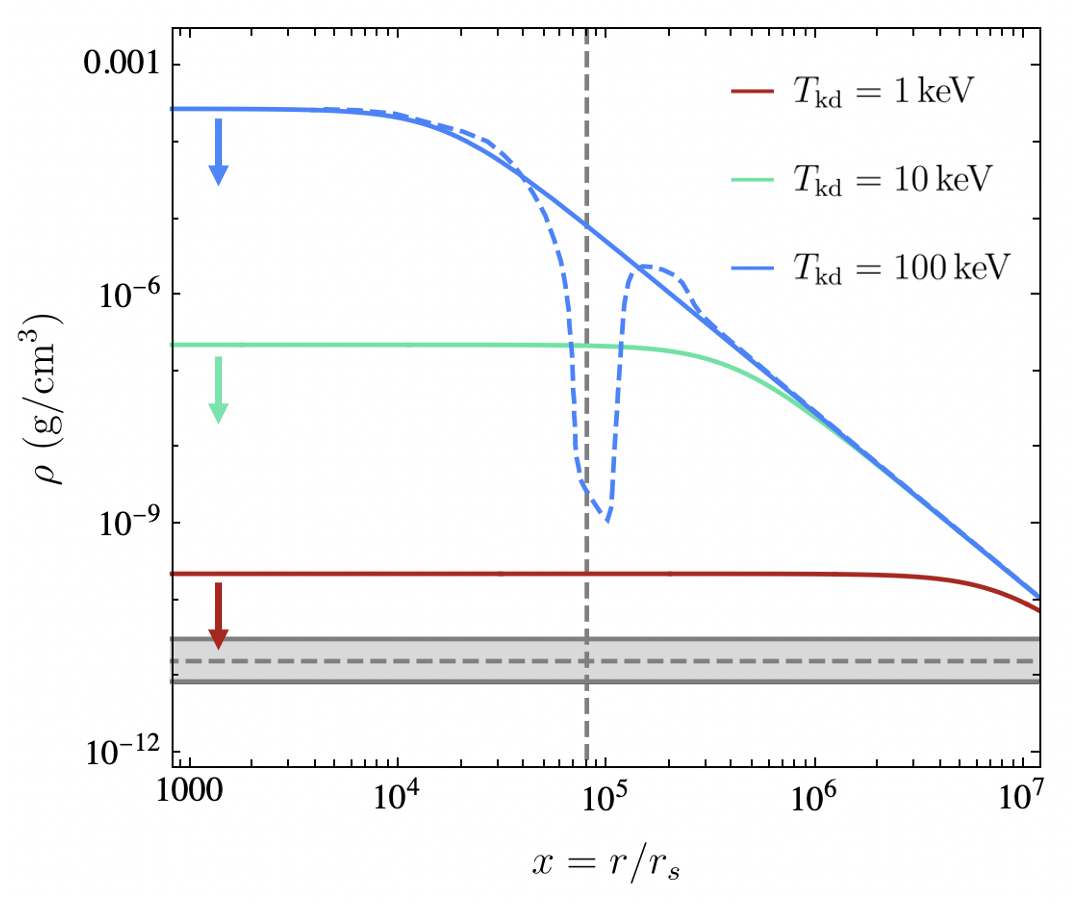
where is the initial radial distance at turn-around, is the initial velocity, is the DM velocity distribution (taken to have a Maxwell-Boltzmann form), is the DM orbital period, and is the initial density profile of Eq. (6). More detail can be found in Appendix A and representative plots are shown in Fig. 1. In the limit of cold DM with small velocities, Eq. (9) reduces to
| (10) |
where we have again introduced the dimensionless radius . In the region where , with the initial spike profile given in Eq. (5), this evaluates explicitly to
| (11) |
with . Thus, the orbital motion of the DM simply serves to amplify the density everywhere by , with the power law scaling intact.
II.1.3 Modification by DM annihilations
For DM that can self-annihilate, the annihilation rate scales as and so will be strongly enhanced in the dense inner core of the halo, resulting in an amplified -ray emission signal [17]. Bounds on the allowed galactic and extragalactic -ray flux then allow us to constrain this hybrid scenario of both PBH and particle DM [24, 26]. In particular for WIMP DM with weak-scale annihilation cross sections, this scenario has been demonstrated to be incompatible with stellar-mass PBHs [25].
Self-annihilations modify the density profile since they impose an upper limit on the DM density [28, 29, 26]
| (12) |
where is the velocity-weighted annihilation cross section. Equating this with Eq. (11) allows us to define the radius below which the power law gives way to a constant density plateau
| (13) |
where . The modified profile is thus
| (14) |
Closer examination has since revealed that instead of a flat annihilation plateau, the spike is flattened to a weak cusp with either for s-wave annihilations [30] or for p-wave [31].
II.2 Growth during Matter Domination
Following matter-radiation equality, accretion becomes efficient and the mass of the DM halo quickly grows to exceed that of the PBH. The dominant process contributing to growth during this era is secondary infall, wherein bound shells of infalling DM are added at successively larger radii [20]. The infall process assumes a self-similar form and for collisionless cold DM results in a power law density profile [20, 21, 25] — the same radial dependence as the mini-spike formed during radiation domination.
To gain some intuition for the origin of this scaling, we follow Ref. [26] and note that the PBH-halo system constitutes an initial overdensity , where is the combined mass of the PBH-halo system and is the background mass in the region. Since density perturbations grow as during matter domination, the mass gravitationally bound to the PBH-halo system grows as
| (15) |
This can amount to a factor growth between matter-radiation equality and the onset of non-linear structure formation around , as confirmed by the numerical simulations of [21]. Meanwhile using that the total energy density dilutes as , the turn-around radius of a DM shell binding at time is
| (16) |
which can be inverted to obtain . Thus we recover the same power law scaling as before, and the density profile of Eq. (5) should be extended beyond
| (17) |
II.3 Modification by Astrophysical Effects
Various astrophysical processes can modify or disrupt the DM spike, particularly at late times after the onset of non-linear structure formation. These include tidal stripping [32, 33], gravitational scattering and other interactions with stars in dense baryonic environments [34, 35, 36], dynamical friction [37, 38], mergers with other BHs [39, 40], and more. Of course there is also the BH-LMXB formation event, which will doubtless affect the profile.
The majority of BH-LMXBs evolve from stellar binaries where one of the stars evolves more quickly than the other and collapses to form a BH [41]. So long as the collapse is not too violent, the bodies remain gravitationally bound and the remaining star begins transferring material to the BH. Though less common, LMXBs can also form through dynamical capture, wherein a star passing close by a BH loses energy through gravitational interactions and becomes gravitationally bound. The likelihood of such an event is highest in dense stellar environments, like globular clusters or galactic centers, as well as when the BH is significantly more massive than the star. The latter criterion is satisfied for our BH-LMXBs of interest, which have (see Table 1).
It is also worth noting that XTE J1118+480 does not seem to have formed through the usual channel. Its stellar component has a metal-rich composition consistent with pollution from a supernova event, which would have ejected the companion from its system of origin [42, 43]. It is thus likely that the constituents of this binary were not born together, instead first encountering one another following this kick and binding dynamically. The BH in XTE J1118+480 need not have originated in stellar collapse, then, but rather may be primordial. If so, then the additional gravitational influence of the massive DM halo as well as the energy dissipation from dynamical friction would have likely aided in the capture process.
It is difficult to estimate the extent to which the DM spike would have been disrupted by tidal stripping during binary formation. Ref. [44] performed numerical studies of PBH-PBH binary formation events and found that tidal stripping could be significant for highly elliptical orbits and comparable masses. Given our small mass ratio and nearly circular orbits, the capture event in our case is likely to be much milder. Numerical simulations are required, however, to make this statement quantitative. Finally, since formation is expected to occur in dense stellar environments, we should also consider gravitational scattering and other interactions with stars. Ref. [45] demonstrated that the highly compact nature of PBH mini-spikes makes them particularly resistant to these sorts of disruptive effects in galactic halos.
We anticipate that dynamical friction and gravitational scattering with the companion star will be the dominant effect modifying the DM profile. Since most of the cold DM particles have speeds less than the star’s orbital speed , they will gain energy through these processes. The energy lost by the star will go into heating up the DM halo, increasing the velocity dispersion and leading to a localized decrease in DM density.
| A0620-00 | XTE J1118+480 | Nova Muscae 1991 | |
|---|---|---|---|
| () | |||
| (km/s) | |||
| (day) | |||
| (ms/yr) | |||
This intuition is confirmed in the numerical simulations of Ref. [37], which demonstrate that dynamical friction can reduce the DM density at the orbital radius by several orders of magnitude. These results were derived in the context of BH-BH binary systems, though, so in Appendix C we generalize to our BH-LMXBs. Using a modified version of the HaloFeedback code of [46], we include in Fig. 1 a representative density profile taking the dynamical friction effect into account. We see that the DM density at the orbital radius is depleted by a factor through these scatterings. In turn, this depletion reduces the effect of dynamical friction.
III Confronting the Data
The companion star traversing the central BH’s DM spike will lose energy to dynamical friction, leading to orbital decay. In Ref. [13], it was argued that this effect could account for the anomalously fast orbital decays of A0620-00 and XTE J1118+480, with and , respectively. We review here how the DM density can be inferred from the orbital decay rate and other precisely measured parameters organized in Table 1.
The star’s energy loss due to this dynamical friction proceeds at a rate [14, 47, 13]
| (18) |
where is the reduced mass, is the DM density at the orbital radius, is the orbital speed, characterizes the fraction of DM particles with speeds less than , and is the Coulomb logarithm. The measured parameters of Table 1 allow us to obtain from the radial velocity and orbital inclination as . We follow Ref. [37] in approximating and . From the total mechanical energy of the system
| (19) |
and Kepler’s law for the orbital period
| (20) |
it follows that
| (21) |
from which we obtain the following expression for the DM density at
| (22) |
Substituting the parameters of Table 1 into this expression, we infer the following densities at the orbital radius: for A0620-00, for XTE J1118+480, and for Nova Muscae 1991. These target densities can then be compared against the PBH mini-spike profiles derived in Sec. II.
Fig. 1 shows sample profiles for the DM mini-spike around a PBH, presuming negligible DM annihilation in accordance with the stringent -ray bounds. Downward arrows indicate that because we have neglected potential halo disruption from tidal stripping during the formation event, these lines should be interpreted as upper bounds on . We see that prior to taking into account halo feedback from dynamical friction, a PBH mini-spike could account for the inferred DM density in XTE J1118+480 so long as the DM has a relatively low333See Ref. [48] for model-building efforts with late-decoupling cold DM, which may help to address the small scale problems of the current cosmological concordance model. kinetic decoupling temperature of . For the benchmark, we also show how the profile may be altered by dynamical friction, using a modified version of the HaloFeedback code of [46]. The observed density depletion at the orbital radius is consistent with the intuition of Sec. II.3, and would make it such that a DM candidate with an earlier kinetic decoupling could account for the inferred density. The plots for A0620-00 and Nova Muscae 1991 are completely analogous to those shown for XTE J1118+480.
If one interprets the anomalously fast orbital decays in these three BH-LMXBs as originating from dynamical friction due to a DM spike, then one is led to the need for some sort of mechanism to build up the DM spike, as stellar-mass BHs of an astrophysical origin are not expected to form DM spikes. In this Letter, we have explored the possibility of a primordial origin for the BHs residing in these LMXBs, as PBHs are expected to efficiently accrete DM, forming ultra-compact high-density mini-spikes. We have computed the mini-spike profile for a cold, collisionless DM candidate and found that for late kinematic decoupling times, this scenario can conceivably account for the density inferred in the dynamical friction hypothesis. We leave to future work the numerical simulations needed to quantify the extent of halo disruption during the formation event.
Acknowledgements
AI thanks Robert Wagoner for suggesting dark matter spikes as a possible topic of interest and for productive conversations.
References
- [1] T. F. J. van Grunsven, P. G. Jonker, F. W. M. Verbunt, and E. L. Robinson, “The mass of the black hole in 1A 0620-00, revisiting the ellipsoidal light curve modelling,” MNRAS 472 no. 2, (Dec., 2017) 1907–1914, arXiv:1708.08209 [astro-ph.HE].
- [2] J. Neilsen, D. Steeghs, and S. D. Vrtilek, “The eccentric accretion disc of the black hole A0620-00,” MNRAS 384 no. 3, (Mar., 2008) 849–862, arXiv:0710.3202 [astro-ph].
- [3] J. I. G. Hernández, R. Rebolo, and J. Casares, “Fast orbital decays of black hole X-ray binaries: XTE J1118+480 and A0620–00,” Mon. Not. Roy. Astron. Soc. 438 no. 1, (2013) L21–L25, arXiv:1311.5412 [astro-ph.HE].
- [4] J. Khargharia, C. S. Froning, E. L. Robinson, and D. M. Gelino, “The Mass of the Black Hole in XTE J1118+480,” APJ 145 no. 1, (Jan., 2013) 21, arXiv:1211.2786 [astro-ph.SR].
- [5] J. Wu et al., “A Dynamical Study of the Black Hole X-ray Binary Nova Muscae 1991,” Astrophys. J. 806 no. 1, (2015) 92, arXiv:1501.00982 [astro-ph.HE].
- [6] J. Wu, J. A. Orosz, J. E. McClintock, I. Hasan, C. D. Bailyn, L. Gou, and Z. Chen, “The Mass of the Black Hole in the X-ray Binary Nova Muscae 1991,” Astrophys. J. 825 no. 1, (2016) 46, arXiv:1601.00616 [astro-ph.HE].
- [7] J. I. González Hernández, L. Suárez-Andrés, R. Rebolo, and J. Casares, “Extremely fast orbital decay of the black hole X-ray binary Nova Muscae 1991,” MNRAS 465 no. 1, (Feb., 2017) L15–L19, arXiv:1609.02961 [astro-ph.SR].
- [8] F. Verbunt and C. Zwaan, “Magnetic braking in low-mass X-ray binaries.,” AAP 100 (July, 1981) L7–L9.
- [9] S. Rappaport, P. C. Joss, and R. F. Webbink, “The evolution of highly compact binary stellar systems.,” APJ 254 (Mar., 1982) 616–640.
- [10] J. I. Gonzalez Hernandez, R. Rebolo, and J. Casares, “The fast spiral-in of the companion star to the black hole XTE J1118+480,” Astrophys. J. Lett. 744 (2012) L25, arXiv:1112.1839 [astro-ph.GA].
- [11] X.-T. Xu and X.-D. Li, “A Circumbinary Disk Model for the Rapid Orbital Shrinkage in Black Hole Low-Mass X-ray Binaries,” Astrophys. J. 859 no. 1, (2018) 46, arXiv:1804.07914 [astro-ph.HE].
- [12] W.-C. Chen and X.-D. Li, “Orbital period decay of compact black hole x-ray binaries: the influence of circumbinary disks?,” Astron. Astrophys. 583 (2015) A108, arXiv:1511.00534 [astro-ph.SR].
- [13] M. H. Chan and C. M. Lee, “Indirect Evidence for Dark Matter Density Spikes around Stellar-mass Black Holes,” Astrophys. J. Lett. 943 no. 2, (2023) L11, arXiv:2212.05664 [astro-ph.HE].
- [14] S. Chandrasekhar, “Dynamical Friction. I. General Considerations: the Coefficient of Dynamical Friction.,” APJ 97 (Mar., 1943) 255.
- [15] S. Chandrasekhar, “Dynamical Friction. II. The Rate of Escape of Stars from Clusters and the Evidence for the Operation of Dynamical Friction.,” APJ 97 (Mar., 1943) 263.
- [16] S. Chandrasekhar, “Dynamical Friction. III. a More Exact Theory of the Rate of Escape of Stars from Clusters.,” APJ 98 (July, 1943) 54.
- [17] P. Gondolo and J. Silk, “Dark matter annihilation at the galactic center,” Phys. Rev. Lett. 83 (1999) 1719–1722, arXiv:astro-ph/9906391.
- [18] L. Sadeghian, F. Ferrer, and C. M. Will, “Dark matter distributions around massive black holes: A general relativistic analysis,” Phys. Rev. D 88 no. 6, (2013) 063522, arXiv:1305.2619 [astro-ph.GA].
- [19] G. D. Quinlan, L. Hernquist, and S. Sigurdsson, “Models of Galaxies with Central Black Holes: Adiabatic Growth in Spherical Galaxies,” APJ 440 (Feb., 1995) 554, arXiv:astro-ph/9407005 [astro-ph].
- [20] E. Bertschinger, “Self-similar secondary infall and accretion in an Einstein-de Sitter universe,” APJ 58 (May, 1985) 39–65.
- [21] K. J. Mack, J. P. Ostriker, and M. Ricotti, “Growth of structure seeded by primordial black holes,” Astrophys. J. 665 (2007) 1277–1287, arXiv:astro-ph/0608642.
- [22] M. Ricotti, “Bondi accretion in the early universe,” Astrophys. J. 662 (2007) 53–61, arXiv:0706.0864 [astro-ph].
- [23] Y. N. Eroshenko, “Dark matter density spikes around primordial black holes,” Astron. Lett. 42 no. 6, (2016) 347–356, arXiv:1607.00612 [astro-ph.HE].
- [24] S. M. Boucenna, F. Kuhnel, T. Ohlsson, and L. Visinelli, “Novel Constraints on Mixed Dark-Matter Scenarios of Primordial Black Holes and WIMPs,” JCAP 07 (2018) 003, arXiv:1712.06383 [hep-ph].
- [25] J. Adamek, C. T. Byrnes, M. Gosenca, and S. Hotchkiss, “WIMPs and stellar-mass primordial black holes are incompatible,” Phys. Rev. D 100 no. 2, (2019) 023506, arXiv:1901.08528 [astro-ph.CO].
- [26] B. Carr, F. Kuhnel, and L. Visinelli, “Black holes and WIMPs: all or nothing or something else,” Mon. Not. Roy. Astron. Soc. 506 no. 3, (2021) 3648–3661, arXiv:2011.01930 [astro-ph.CO].
- [27] A. M. Green and B. J. Kavanagh, “Primordial Black Holes as a dark matter candidate,” J. Phys. G 48 no. 4, (2021) 043001, arXiv:2007.10722 [astro-ph.CO].
- [28] P. Ullio, L. Bergstrom, J. Edsjo, and C. G. Lacey, “Cosmological dark matter annihilations into gamma-rays - a closer look,” Phys. Rev. D 66 (2002) 123502, arXiv:astro-ph/0207125.
- [29] P. Scott and S. Sivertsson, “Gamma-Rays from Ultracompact Primordial Dark Matter Minihalos,” Phys. Rev. Lett. 103 (2009) 211301, arXiv:0908.4082 [astro-ph.CO]. [Erratum: Phys.Rev.Lett. 105, 119902 (2010)].
- [30] E. Vasiliev, “Dark matter annihilation near a black hole: Plateau vs. weak cusp,” Phys. Rev. D 76 (2007) 103532, arXiv:0707.3334 [astro-ph].
- [31] S. L. Shapiro and J. Shelton, “Weak annihilation cusp inside the dark matter spike about a black hole,” Phys. Rev. D 93 no. 12, (2016) 123510, arXiv:1606.01248 [astro-ph.HE].
- [32] M. P. Hertzberg, E. D. Schiappacasse, and T. T. Yanagida, “Implications for dark matter direct detection in the presence of LIGO-motivated primordial black holes,” Phys. Lett. B 807 (2020) 135566, arXiv:1910.10575 [astro-ph.CO].
- [33] A. Schneider, L. Krauss, and B. Moore, “Impact of Dark Matter Microhalos on Signatures for Direct and Indirect Detection,” Phys. Rev. D 82 (2010) 063525, arXiv:1004.5432 [astro-ph.GA].
- [34] P. Ullio, H. Zhao, and M. Kamionkowski, “A Dark matter spike at the galactic center?,” Phys. Rev. D 64 (2001) 043504, arXiv:astro-ph/0101481.
- [35] G. Bertone and D. Merritt, “Time-dependent models for dark matter at the Galactic Center,” Phys. Rev. D 72 (2005) 103502, arXiv:astro-ph/0501555.
- [36] S. L. Shapiro and D. C. Heggie, “Effect of stars on the dark matter spike around a black hole: A tale of two treatments,” Phys. Rev. D 106 no. 4, (2022) 043018, arXiv:2209.08105 [astro-ph.GA].
- [37] B. J. Kavanagh, D. A. Nichols, G. Bertone, and D. Gaggero, “Detecting dark matter around black holes with gravitational waves: Effects of dark-matter dynamics on the gravitational waveform,” Phys. Rev. D 102 no. 8, (2020) 083006, arXiv:2002.12811 [gr-qc].
- [38] A. Coogan, G. Bertone, D. Gaggero, B. J. Kavanagh, and D. A. Nichols, “Measuring the dark matter environments of black hole binaries with gravitational waves,” Phys. Rev. D 105 no. 4, (2022) 043009, arXiv:2108.04154 [gr-qc].
- [39] H. Nishikawa, E. D. Kovetz, M. Kamionkowski, and J. Silk, “Primordial-black-hole mergers in dark-matter spikes,” Phys. Rev. D 99 no. 4, (2019) 043533, arXiv:1708.08449 [astro-ph.CO].
- [40] P. Jangra, B. J. Kavanagh, and J. M. Diego, “Impact of dark matter spikes on the merger rates of Primordial Black Holes,” JCAP 11 (2023) 069, arXiv:2304.05892 [astro-ph.CO].
- [41] X.-D. Li, “Formation of Black Hole Low-Mass X-ray Binaries,” New Astron. Rev. 64-66 (2015) 1–6, arXiv:1502.07074 [astro-ph.HE].
- [42] J. I. Gonzalez Hernandez, R. Rebolo, G. Israelian, E. T. Harlaftis, A. V. Filippenko, and R. Chornock, “XTE J1118+480: A Metal-Rich Black Hole Binary in the Galactic Halo,” Astrophys. J. Lett. 644 (2006) L49–L52, arXiv:astro-ph/0605107.
- [43] J. I. G. Hernandez, R. Rebolo, G. Israelian, A. V. Filippenko, R. Chornock, N. Tominaga, H. Umeda, and K. Nomoto, “Chemical Abundances of the Secondary Star in the Black Hole X-ray Binary XTE J1118+480,” Astrophys. J. 679 (2008) 732, arXiv:0801.4936 [astro-ph].
- [44] B. J. Kavanagh, D. Gaggero, and G. Bertone, “Merger rate of a subdominant population of primordial black holes,” Phys. Rev. D 98 no. 2, (2018) 023536, arXiv:1805.09034 [astro-ph.CO].
- [45] M. Sten Delos and J. Silk, “Ultradense dark matter haloes accompany primordial black holes,” Mon. Not. Roy. Astron. Soc. 520 no. 3, (2023) 4370–4375, arXiv:2210.04904 [astro-ph.CO].
- [46] B. J. Kavanagh, “Halofeedback [code v0.9],” https://github.com/bradkav/HaloFeedback, 2020.
- [47] F. Dosopoulou, “Dynamical friction in dark matter spikes: corrections to Chandrasekhar’s formula,” arXiv:2305.17281 [astro-ph.HE].
- [48] T. Bringmann, H. T. Ihle, J. Kersten, and P. Walia, “Suppressing structure formation at dwarf galaxy scales and below: late kinetic decoupling as a compelling alternative to warm dark matter,” Phys. Rev. D 94 no. 10, (2016) 103529, arXiv:1603.04884 [hep-ph].
- [49] M. Cirelli, E. Moulin, P. Panci, P. D. Serpico, and A. Viana, “Gamma ray constraints on Decaying Dark Matter,” Phys. Rev. D 86 (2012) 083506, arXiv:1205.5283 [astro-ph.CO].
- [50] S. Ando and K. Ishiwata, “Constraints on decaying dark matter from the extragalactic gamma-ray background,” JCAP 05 (2015) 024, arXiv:1502.02007 [astro-ph.CO].
- [51] Fermi-LAT Collaboration, M. Ackermann et al., “The spectrum of isotropic diffuse gamma-ray emission between 100 MeV and 820 GeV,” Astrophys. J. 799 (2015) 86, arXiv:1410.3696 [astro-ph.HE].
- [52] J. Binney and S. Tremaine, Galactic Dynamics: Second Edition. 2008.
Appendix A Modification by DM Orbital Motion
In this appendix, we determine how the initial density profile of Eq. (6) is modified by the finite velocities and orbital motion of the DM. Following the treatment of Refs. [23, 26], we begin by using conservation of phase space to write
| (23) |
where is the initial radial distance from the PBH at turn-around, is the initial velocity, is the DM orbital period, and is the initial density profile of Eq. (6). We take the DM velocity to have a Maxwell-Boltzmann distribution,
| (24) |
where is the DM temperature, which depends on radial position as
| (25) |
For convenience, we normalize radii to and define the dimensionless , . The initial energy of a DM particle then reads
| (26) |
while the energy at an arbitrary time is
| (27) |
which we have simplified using the conservation of angular momentum . Conservation of energy then allows us to identify the radial speed as
| (28) |
and the orbital period as
| (29) |
Writing and performing the integral over , we arrive at the expression
| (30) |
where we have defined
| (31) |
which takes values . For each , we will first perform the integral over . The range of can be found by demanding that , corresponding to bound orbits, and that the integrand of Eq. (28) be positive. There are two sub-cases, depending on whether or .
Case 1) : Here, the particle initially moves outward, corresponding to the situation where at turn-around. We have already demonstrated that this regime is not relevant for our stellar-mass PBHs of interest, and so we will not consider it further beyond commenting that this case is what gives rise to the intermediate power law scaling found in Ref. [23]. We thus do not expect to see this behavior in our density profile.
Case 2) : Here, the particle moves always inwards since at turn-around. The limits of integration for are
| (32) |
Though in Fig. 1 we evaluate Eq. (23) numerically with the distribution of Eq. (24), for the sake of obtaining an analytic expression here we can approximate , which is reasonable since we are thoroughly in the regime where potential energy dominates kinetic. In this case, Eq. (30) becomes444Technically, the upper limit should be . This is sufficiently large, however, that little error is incurred in approximating .
| (33) |
In the region where , with the initial mini-spike profile given in Eq. (5), this evaluates to
| (34) |
with . Thus, we see that this effect serves to amplify the density everywhere by . In particular, the power law scaling is retained.
Appendix B Constraints on DM Annihilations
DM self-annihilations in the density spike proceed at a rate [24]
| (35) |
which for the density profile of Eq. (14) can be explicitly evaluated as
| (36) |
The -ray flux from these annihilations contributes to both galactic and extragalactic backgrounds, and so can be compared against measurements of the isotropic -ray flux.
Following Ref. [49], we resolve the total flux into galactic and extragalactic components
| (37) |
Note that although the galactic contribution is not isotropic (hence the differential solid angle ), its minimum still constitutes an irreducible background contribution to the isotropic flux. Explicitly, these fluxes are [49, 24]
| (38) |
and
| (39) |
where describes the number of photons per unit energy produced in the annihilation channel. The first integral is taken over the line of sight (l.o.s.) while the second is taken over all redshifts. We also note that the density appearing in the second expression is the total DM density today, and the optical depth appears in the second integral to account for the attenuation of high-energy -rays.
Following Ref. [24], we will utilize the fact that these expressions are identical to those for decaying DM provided we make the substitution
| (40) |
The idea then is to translate the experimental bounds for decaying DM to constraints on . In particular, we consider the bounds of Ref. [50] derived from data from the Large Area Telescope (LAT) onboard the Fermi satellite [51]. The strongest bounds on DM lifetime for much of the mass range come from the channel and constrain . If we take for example , then for a PBH we must demand .
Such small cross sections correspond to values which are much too large to bring us within range of our target DM densities. The smaller values needed to explain the anomalous orbital decays would result in an overproduction of -rays, and so we do not include them in Fig. 1. We remark, however, that if there are other astrophysical effects which reduce DM density in the halo, such as tidal stripping during the LMXB formation event, then these annihilation density profiles may become relevant.
Appendix C Feedback from Dynamical Friction
Here we analyze how dynamical friction and heating due to gravitational scattering with the companion star redistribute DM density in the halo. We follow the strategy of Ref. [37], who presented an analogous calculation in the context of a BH binary system. The idea is to track how the phase space distribution of the DM evolves as energy is injected by the orbiting compact object.
Given the parameters in Table 1, it is justified to assume the orbital parameters to evolve on a timescale much greater than the orbital period . We also take the DM halo to be spherically symmetric and isotropic, a reasonable assumption given that both LMXB systems have nearly circular orbits, with very little eccentricity. These assumptions allows us to characterize the DM by an equilibrium phase space distribution
| (41) |
which is a function of energy per unit mass alone,
| (42) |
The Newtonian gravitational potential receives contributions from both the PBH and the DM halo,
| (43) |
For a given halo density profile , the corresponding can be obtained from the Poisson equation by first computing the mass enclosed in a radius
| (44) |
and then computing the potential as
| (45) |
The distribution function is then given by Eddington’s inversion formula [52]
| (46) |
Though the DM halo in its entirety is more massive than the PBH by the end of matter domination, the mass contained within the orbital radius of the companion star is smaller by several orders of magnitude. Thus, it is appropriate to approximate the gravitational potential by that of the PBH, . This is convenient since it eliminates the need to update as the halo is perturbed. Further, it allows us to evaluate Eq. (46) explicitly. Presuming a generic power law profile , we can write
| (47) |
in which case
| (48) |
This should be regarded as the “initial” DM phase space distribution, not in a temporal sense but rather in that it describes the distribution before the gravitational interactions with the companion star are taken into account. Given a distribution function , the density profile can be obtained as
| (49) |
with . The idea then is to evolve and then substitute the result into Eq. (49) in order to find the final density profile in the halo.
To that end, we introduce the density of states , computed as
| (50) |
This allows us to write the number of particles with energy in the interval as
| (51) |
Let be the probability per orbit for a DM particle of energy to scatter with the companion star, gaining an energy in the process. Then we can write the change in the number of particles with energy over the course of a single orbit as
| (52) |
where the first term describes the depletion of particles initially of energy that have been upscattered to and the second term describes replenishment from particles of initial energy upscattered to . Using Eq. (51), the change in the distribution function becomes
| (53) |
To proceed further, we need to know the explicit form of . This can be derived using results in appendix L of Ref. [52]. Consider a scattering event between the orbiting companion star and a DM particle with impact parameter , the geometry for which is depicted in Fig. 7 of [37]. Due to this encounter, the parallel component of the star’s velocity changes as
| (54) |
where we have approximated the DM’s velocity as negligible relative to that of the star and defined as the impact parameter required to produce a deflection of the DM, . The resultant change in the star’s energy is , which by conservation of energy implies that the DM particle acquires an energy of
| (55) |
This enters into the scattering probability as
| (56) |
where we have introduced as the root of the remaining delta function. From this, we see that the spatial integration should be carried out over a torus with major and minor radii and , respectively. After performing the trivial integral over the azimuthal angle, it is convenient to perform a change of variables , related as
| (57a) | |||
| (57b) |
By computing the Jacobian for the transformation, one can show that . Using the delta function to perform the integral, the result is
| (58) |
Since we are in the regime , we can expand each factor in the integrand in a power series in , keeping only the leading terms. Evaluating the integral and using Eq. (50) to simplify the answer, we find to leading order
| (59) |
Using and as well as writing things in terms of the dimensionless radii introduced previously, the scattering probability takes the very compact form
| (60) |
Now equipped with an expression for , we return to Eq. (53). Since the system evolves on a timescale much longer than the orbital frequency, we can convert this to a differential equation by writing , where is the orbital period. Solving with the aid of a modified version of the HaloFeedback code of [46], we plot a sample result in Fig. 1. Note that for simplicity, we have considered the companion star orbiting at a fixed radius. For a self-consistent treatment, however, we should really solve the coupled system of differential equations for the evolving orbital radius and . Since the required numerics are beyond the scope of this work, we maintain self-consistency by restricting evolution to orbits, corresponding to a change in .