Tailoring Bound State Geometry in High-Dimensional Non-Hermitian Systems
Abstract
It is generally believed that the non-Hermitian effect (NHSE), due to its non-reciprocal nature, creates barriers for the appearance of impurity bound states. In this paper, we find that in two and higher dimensions, the presence of geometry-dependent skin effect eliminates this barrier such that even an infinitesimal impurity potential can confine bound states in this type of non-Hermitian systems. By examining bound states around Bloch saddle points, we find that non-Hermiticity can disrupt the isotropy of bound states, resulting in concave dumbbell-shaped bound states. Our work reveals a geometry transition of bound state between concavity and convexity in high-dimensional non-Hermitian systems.
Introduction.— The non-Hermitian Hamiltonian serves as an effective tool for describing open systems that interact with environments [1, 2, 3, 4, 5, 6, 7, 8, 9, 10, 11, 12, 13, 14, 15]. Recently, non-Hermitian band systems have drawn much attention due to their intriguing phenomena that surpass the traditional Bloch band framework [16, 17]. A representative phenomenon is the non-Hermitian skin effect (NHSE) [18, 19, 20, 21, 22, 23, 24, 25, 26, 27, 28, 29, 30, 31, 32, 33, 34, 35, 36, 37, 38, 39, 40, 41, 42]. In one dimension, the NHSE is characterized by a large number of eigenstates localized at the ends of an open chain, well understood in the generalized Bloch band framework [20, 23, 27, 29, 35]. In two and higher dimensions, the NHSE exhibits more complexity due to the interplay between mode localization and open boundary geometries. Particularly, the NHSE may disappear under certain geometry but reappear under others. This dimensionality enriched phenomenon is referred to as the geometry-dependent skin effect (GDSE) [39, 43, 44, 45, 46, 47, 48, 49, 50].
The topic of impurity states is fundamental in Hermitian systems and has been extensively studied due to its wide-ranging applications. For example, the Kondo effect is induced by magnetic impurities in metals [51], and Yu-Shiba-Rusinov impurity bound states appear in s-wave superconductors [52, 53, 54]. Recently, the investigation of impurity states in non-Hermitian settings, especially their interplay with NHSE, has revealed various new physical phenomena [55, 56]. A key aspect is that, NHSE creates barriers for the formation of impurity bound states due to its non-reciprocal nature [57, 58]. Consequently, a finite impurity potential is necessary to induce a bound state when NHSE is present [59]. However, these phenomena have primarily been studied in 1D non-Hermitian systems, it is still unclear whether impurity states can exhibit new properties in higher dimensions. Additionally, NHSE presents new characteristics in higher dimensions [60, 39, 61], such as GDSE. The potential for impurity states to exhibit novel behaviors in interaction with these emerging forms of NHSE in higher dimensions remains a significant and largely unexplored research gap.
In this paper, we find that in the presence of GDSE, the impurity potential exhibits a zero threshold for the emergence of bound states, which is demonstrated by establishing an exact mapping between the bound state energy and the required impurity potential. Specifically, even an infinitesimal impurity potential can confine bound states in a non-Hermitian system exhibiting GDSE. A key reason is that the GDSE ensures the presence of Bloch saddle points, which further eliminates the barriers for the formation of impurity bound states.
In two and higher dimensions, the geometry of equal amplitude contour of wavefunction introduces a new characteristic for non-Hermitian impurity bound states. Here, we determine the geometry of bound states utilizing a mathematical tool of amoeba. We find that in two dimensions, the impurities can host anisotropic, concave bound states. This geometry feature is in sharp contrast with that observed in Hermitian systems, where bound states are typically isotropic and convex. Furthermore, we reveal a geometric transition from convexity to concavity in the bound states by manipulating the impurity potential. This transition is characterized using our method and is observable in experimental setups, such as through the local density of states patterns.
A general theory of bound states in non-Hermitian systems.— We start from a general tight-binding Hamiltonian with finite range couplings in two dimensions,
| (1) |
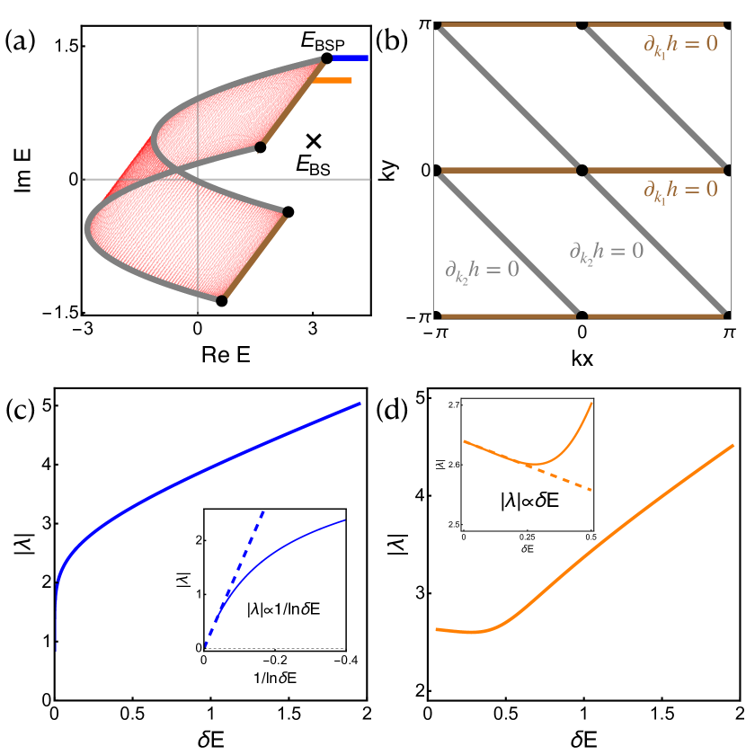
where , represents the position of lattice site, and indicates the hopping strength. The Bloch spectrum is formed by the eigenvalues of as and scan over the entire Brillouin zone (BZ), which we denote by [red dots in Fig. 1(a)].
To generate an impurity bound state, we place a single impurity potential of strength at the origin of the lattice, where the coordinate is set to . The impurity potential takes the form
| (2) |
One can tune the impurity strength such that the excited bound state has an energy appearing beyond the region of [the black cross in Fig. 1(a)]. Utilizing Green’s function method, the wavefunction of this bound state can be analytically obtained as [62]
| (3) |
where is the Green’s function, is given by Eq. (1), and is determined by the wavefunction’s normalization condition. Setting and to zero in Eq. (3), the relationship between the bound state energy and the required impurity strength is established as
| (4) |
Under PBC, the Green’s function on the right-hand side of Eq. (4) can be expanded under Bloch basis as an integral form, and thus the relationship becomes
| (5) |
Typically, a state with energy within a continuum spectrum is expressed as a scattering state. Correspondingly, the energy of a bound state should lie outside the region of . The critical point, where the bound state energy merges with the PBC continuous spectrum, signifies a phase transition. This phase transition determines the minimum impurity strength required to create bound states. Consequently, we can define the set of minimum impurity strengths as
| (6) |
where represents the boundary of PBC continuum spectrum, and denotes a spectral boundary point. We define the impurity strength threshold as the minimum absolute value in the set . The Bloch saddle points (BSPs), denoted as , refer to the saddle points in the BZ where the relation holds: for . In the following, we demonstrate that zero threshold of impurity strength is ensured by the presence of BSPs in the Bloch spectrum .
The critical response to impurity potential near BSPs.— Here, we examine the excitation around the BSP energy, which is assumed to be located at the spectrum boundary, denoted by . The lattice Bloch Hamiltonian can be expanded at the BSP as , where and are the derivations from the BSP momentum, and represent expansion coefficients. It’s worth noting that the linear and terms have been omitted since is a BSP. The cross term can be eliminated through a proper momentum basis rotation such that certain conditions are satisfied [63]. Therefore, the expanded Hamiltonian around a BSP can be classified according to the coefficients . For demonstration, we utilize the following concrete lattice Hamiltonian,
| (7) |
With a weak impurity potential, the excited bound state energy shifts slightly from the BSP energy , i.e., . Substituting Eq. (7) into Eq. (5), when , the relationship between the impurity strength and the bound state energy becomes (see details in Supplementary Material [64]): , where the parameters and . Here, diverges asymptotically as when , which is expressed as:
| (8) |
Here, we emphasize that according to the relation in Eq. (8), the excited bound state energy is highly sensitive to the impurity potential near the BSP energy, which is verified in Fig. 1(c). This stands in stark contrast to the linear response relation for excitations near the regular spectrum boundary energy, shown in Fig. 1(d). It can be expected that such response sensitivity to impurities can be utilized to detect the existence of BSPs in experiments in higher-dimensional non-Hermitian systems [46, 47, 48]. It follows from Eq. (8) that as approaches zero, the required impurity potential also tends to zero, indicating a zero threshold for the impurity potential at the BSPs. We conclude that the existence of BSPs leads to the zero threshold of impurity potential.
The numerical verification for the zero threshold at BSPs is illustrated in Fig. 1. As the bound state energy approaches the BSP energy along the blue line in Fig. 1(a), the required impurity potential decreases to zero, as shown in Fig. 1(c). As a comparison, when moves toward a regular spectral boundary energy, e.g., along the orange trajectory in Fig. 1(a), the associated impurity potential approaches a finite value, as illustrated in Fig. 1(d). Dashed lines in Figs. 1(c) and (d) indicate the asymptotic behavior near the boundary.
A natural question arises: what kind of systems can ensure the existence of BSPs in higher dimensions? The answer lies in systems that exhibit GDSE. In GDSE, there are two special directions, in which the momenta are denoted by and , respectively. When boundary cuts are made along these directions, the resulting open boundary eigenstates manifest as Bloch waves. By imposing the open boundary conditions along the direction and periodic boundary conditions along the direction, momentum is conserved, allowing the Hamiltonian to be treated as a 1D -subsystem for a fixed . Since the system has no skin effect in the direction, the energy spectrum forms an arc along this direction. The endpoints of this arc satisfy . As varies from to , these endpoints form two lines [the brown lines shown in Fig. 1(b)]. Similarly, two additional lines can be obtained for the direction [the black lines illustrated Fig. 1(b)]. At the intersections of these four lines, the BSP conditions, for , are satisfied. Thus, these intersections correspond to four BSPs within the BZ. An illustrative example with is presented in Fig. 1(b), where the intersections are denoted by black dots.
Tailoring the geometry of bound states.— According to Eq. (3), the bound state wave function is determined by Green’s function. The Green’s function can be expressed in an integral form with the Hamiltonian given by Eq. (1):
| (9) |
Here, we have extended the real momentum to the complex value and defined for . Under PBC, the integral contour is the BZ (), a torus in space, which we denote as . To compute this double integral, we adopt a step-by-step integration strategy. Firstly, we evaluate the first integral using the residue theorem. Secondly, for the second integral, as we are primarily concerned with the asymptotic behavior of the wave function far from the impurity (), we can use the saddle-point approximation to handle the second integral, resulting in [64]:
| (10) |
Here, and the complex momentum vector is a saddle point of the exponent in Eq. 9 , depending on the spatial direction . Eq. (10) demonstrates that the bound state wave function exhibits exponential behavior characterized by the complex momentum along a fixed direction , resulting in anisotropy in space. Therefore, we define the characteristic localization that satisfies the relation: , which is further expressed as:
| (11) |
Here, forms a closed loop as changes, which characterizes the localization behavior and describes the geometric shape of impurity bound states.
For a fixed direction , the complex momentum is determined by solving specific constraints (see details in the Supplementary Material [64]). The first constraint is the bulk characteristic equation,
| (12) |
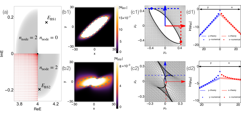
The set of imaginary parts of the complex momentum that satisfy the characteristic equation in Eq. (12) is termed amoeba, as represented by the gray regions in Figs. 2(c1) and (c2). Since [65], the corresponding amoeba always features a central hole [66], as shown by the blank region in Fig. 2(c1) and (c2). Moreover, by solving Eq. (12), or can be expressed as a function of the other. By applying the saddle point approximation to the exponential factor in Eq. (10) and utilizing the implicit function theorem , the second constraint can be derived as
| (13) |
So far, for impurity bound state, the first constraint in Eq. (12) relates the solution domain of () to the mathematical term amoeba; the second constraint in Eq. (13), combined with Eq.(12), locates several isolated points on amoeba. By changing the spatial direction , will form a closed loop which corresponds to a mathematical concept called the amoeba’s contour [67, 68, 69]. As shown in Figs. 2(c1) and (c2), the amoeba’s contours are represented by the black curves. The constraint given by Eq. (13) is a homogeneous function of and , which depends solely on the spatial direction . Therefore, the bound state wavefunction exhibits exponential localization away from the impurity site, while it is not isotropic in real space. Furthermore, by applying implicit function theorem to Eq. (13), it can be transformed into the form . Notably, this is a complex equation, and by taking its imaginary part, we obtain
| (14) |
This formula indicates that the inverse localization length of bound states along each spatial direction is determined by the value on the amoeba’s contour, where the tangent direction is perpendicular to .
As a result, for a fixed direction , we can determine the inverse localization length using Eq. 12 and Eq. 13. By varying the spatial direction , we find that the set of forms a closed loop on the amoeba, corresponding to the amoeba’s contour. Additionally, Eq. 14 indicates that the tangent direction of is perpendicular to .
By substituting the values of into Eq. (11), we can determine the geometric shape of the bound state. As illustrated in Fig. 2(a), the bound states with energies and are illustrated in Figs. 2(b1) and (b2), respectively. Their corresponding amoebas are calculated in Figs. 2(c1) and (c2). To further delve into the localization behaviors, we plot and for these two bound states in Figs 2(d1) and (d2). According to our conclusion, the decay rate of bound states along the and directions are determined by the corresponding points on the amoeba’s contours, which are illustrated by the red and blue dots in Figs 2(c1) and (c2). As the numerical verifications in Figs 2(d1) and (d2), the corresponding slopes at the amoeba’s contour points are represented by the red and blue solid lines, matching exactly with the numerical bound state wavefunctions, as indicated by the red and blue dots.
We conclude that the amoeba’s contour encodes the localization lengths of the bound state along each spatial direction. Therefore, the characteristic geometric shape of the bound state wavefunction can be tailored by the amoeba’s contour. Moreover, since the amoeba’s contour is determined by the bulk Hamiltonian of the system, it is expected that non-Hermitian systems can host unique bound state geometric features beyond those observed in conventional Hermitian systems.
Geometry transition of bound state under weak impurity analysis.—
Here, by perturbation analysis with a weak impurity potential excitation, we demonstrate a geometry transition unique to higher-dimensional non-Hermitian systems. As previously mentioned, the non-Hermitian systems having GDSE ensure the existence of BSPs, where the bound state can be excited by an infinitesimal impurity potential. Therefore, GDSE system provides a platform to examine the bound state geometry features with a weak impurity excitation. As we established before, the bound state geometry can be tailored by the amoeba’s contour. The latter is fully determined by the characterization equation . Here, we only consider its expansion near BSP energy , which is generally expressed as:
| (15) |
Here, the linear term of and vanishes due to the BSP condition, and cross term is omitted for simplicity [64]. By applying the constraints in Eq. (12) and Eq. (13), we can derive an algebraic curve of order 8 that describes the amoeba’s contour (see details in Supplementary Material [64]). Based on Eq. (11), we ultimately obtain an algebraic curve that features the bound state geometry shape:
| (16) |
where . This curve describes the localization length of the wave function along different directions and determines the shape of the bound states.
When , the Hamiltonian reduces to Hermitian, and the geometry curve collapses into a circle, given by
| (17) |
Therefore, the shape of the bound state in Hermitian limit is always circular (or elliptical due to a scaling factor on or ). However, when , as illustrated in Fig.2(a), varying leads to a transition in the shape of the bound state from a regular convex curve in Fig. 2(b1) to a concave and dumbbell-like curve in Fig. 2(b2), which is unique to higher-dimensional non-Hermitian systems. This transition corresponds to the transition of the amoeba’s contour from a regular curve in Fig. 2(c1) to an irregular curve with multiple singular nodes in Fig. 2(c2). Here, a curve is considered as convex if and only if it exhibits positive or negative curvature tracing along its path, while a singular node is defined as the singular point at which the curve intersects with itself. The nodes always appear in pairs due to reciprocity symmetry in GDSE systems. We show that concave geometry of bound states appears if and only if the phase or falls within the range of . The proof is detailed in Supplementary Material [64]. For weak impurity excitation near BSPs, when or , as indicated by the gray region in Fig. 2(a), the amoeba contour exhibits two nodes. Consequently, the geometry of the corresponding bound state wave function is concave.
Conclusion.— In summary, we investigate the characteristics of impurity-induced bound states in 2D non-Hermitian lattice systems. Our findings indicate that existence of BSPs can eliminate the threshold for the formation of impurity bound states. Notably, in a system with GDSE, even an infinitesimal impurity potential can generate bound states near the BSP energy. Such systems serve as optimal platforms for the investigation of bound states with weak excitations near BSPs. The geometry of these bound state wavefunctions is concave and anisotropic, in sharp contrast with convex, isotropic shapes observed in Hermitian systems. The existence of such bound states demonstrates that non-Hermitian properties can significantly enrich the geometric configurations of bound states.
References
- Rotter [2009] Ingrid Rotter, “A non-hermitian hamilton operator and the physics of open quantum systems,” Journal of Physics A: Mathematical and Theoretical 42, 153001 (2009).
- Diehl et al. [2011] Sebastian Diehl, Enrique Rico, Mikhail A. Baranov, and Peter Zoller, “Topology by dissipation in atomic quantum wires,” Nature Physics 7, 971–977 (2011).
- Malzard et al. [2015] Simon Malzard, Charles Poli, and Henning Schomerus, “Topologically protected defect states in open photonic systems with non-hermitian charge-conjugation and parity-time symmetry,” Phys. Rev. Lett. 115, 200402 (2015).
- Dalibard et al. [1992] Jean Dalibard, Yvan Castin, and Klaus Mølmer, “Wave-function approach to dissipative processes in quantum optics,” Phys. Rev. Lett. 68, 580–583 (1992).
- Regensburger et al. [2012] Alois Regensburger, Christoph Bersch, Mohammad-Ali Miri, Georgy Onishchukov, Demetrios N. Christodoulides, and Ulf Peschel, “Parity–time synthetic photonic lattices,” Nature 488, 167–171 (2012).
- Gao et al. [2015] T. Gao, E. Estrecho, K. Y. Bliokh, T. C. H. Liew, M. D. Fraser, S. Brodbeck, M. Kamp, C. Schneider, S. Höfling, Y. Yamamoto, F. Nori, Y. S. Kivshar, A. G. Truscott, R. G. Dall, and E. A. Ostrovskaya, “Observation of non-Hermitian degeneracies in a chaotic exciton-polariton billiard,” Nature 526, 554–558 (2015).
- Feng et al. [2017] Liang Feng, Ramy El-Ganainy, and Li Ge, “Non-Hermitian photonics based on parity–time symmetry,” Nature Photonics 11, 752–762 (2017).
- El-Ganainy et al. [2018] Ramy El-Ganainy, Konstantinos G. Makris, Mercedeh Khajavikhan, Ziad H. Musslimani, Stefan Rotter, and Demetrios N. Christodoulides, “Non-Hermitian physics and PT symmetry,” Nature Physics 14, 11–19 (2018).
- Miri and Alù [2019] Mohammad-Ali Miri and Andrea Alù, “Exceptional points in optics and photonics,” Science 363, eaar7709 (2019).
- Özdemir et al. [2019] Ş. K. Özdemir, S. Rotter, F. Nori, and L. Yang, “Parity–time symmetry and exceptional points in photonics,” Nature Materials 18, 783–798 (2019).
- Kozii and Fu [2017] Vladyslav Kozii and Liang Fu, “Non-Hermitian Topological Theory of Finite-Lifetime Quasiparticles: Prediction of Bulk Fermi Arc Due to Exceptional Point,” arXiv:1708.05841 (2017).
- Shen and Fu [2018] Huitao Shen and Liang Fu, “Quantum oscillation from in-gap states and a non-hermitian landau level problem,” Phys. Rev. Lett. 121, 026403 (2018).
- Nagai et al. [2020] Yuki Nagai, Yang Qi, Hiroki Isobe, Vladyslav Kozii, and Liang Fu, “DMFT Reveals the Non-Hermitian Topology and Fermi Arcs in Heavy-Fermion Systems,” Phys. Rev. Lett. 125, 227204 (2020).
- Song et al. [2019] Fei Song, Shunyu Yao, and Zhong Wang, “Non-hermitian skin effect and chiral damping in open quantum systems,” Phys. Rev. Lett. 123, 170401 (2019).
- Ashida et al. [2020] Yuto Ashida, Zongping Gong, and Masahito Ueda, “Non-hermitian physics,” Advances in Physics 69, 249–435 (2020), doi: 10.1080/00018732.2021.1876991.
- Shen et al. [2018] Huitao Shen, Bo Zhen, and Liang Fu, “Topological Band Theory for Non-Hermitian Hamiltonians,” Phys. Rev. Lett. 120, 146402 (2018).
- Kawabata et al. [2019] Kohei Kawabata, Ken Shiozaki, Masahito Ueda, and Masatoshi Sato, “Symmetry and Topology in Non-Hermitian Physics,” Phys. Rev. X 9, 041015 (2019).
- Lee [2016] Tony E. Lee, “Anomalous edge state in a non-hermitian lattice,” Phys. Rev. Lett. 116, 133903 (2016).
- Martinez Alvarez et al. [2018] V. M. Martinez Alvarez, J. E. Barrios Vargas, and L. E. F. Foa Torres, “Non-hermitian robust edge states in one dimension: Anomalous localization and eigenspace condensation at exceptional points,” Phys. Rev. B 97, 121401(R) (2018).
- Yao and Wang [2018] Shunyu Yao and Zhong Wang, “Edge States and Topological Invariants of Non-Hermitian Systems,” Phys. Rev. Lett. 121, 086803 (2018).
- Kunst et al. [2018] Flore K. Kunst, Elisabet Edvardsson, Jan Carl Budich, and Emil J. Bergholtz, “Biorthogonal Bulk-Boundary Correspondence in Non-Hermitian Systems,” Phys. Rev. Lett. 121, 026808 (2018).
- Yao et al. [2018] Shunyu Yao, Fei Song, and Zhong Wang, “Non-Hermitian Chern Bands,” Phys. Rev. Lett. 121, 136802 (2018).
- Yokomizo and Murakami [2019] Kazuki Yokomizo and Shuichi Murakami, “Non-Bloch Band Theory of Non-Hermitian Systems,” Phys. Rev. Lett. 123, 066404 (2019).
- Lee and Thomale [2019] Ching Hua Lee and Ronny Thomale, “Anatomy of skin modes and topology in non-Hermitian systems,” Phys. Rev. B 99, 201103(R) (2019).
- Lee et al. [2019] Ching Hua Lee, Linhu Li, and Jiangbin Gong, “Hybrid Higher-Order Skin-Topological Modes in Nonreciprocal Systems,” Phys. Rev. Lett. 123, 016805 (2019).
- Longhi [2019] Stefano Longhi, “Probing non-hermitian skin effect and non-bloch phase transitions,” Phys. Rev. Res. 1, 023013 (2019).
- Zhang et al. [2020] Kai Zhang, Zhesen Yang, and Chen Fang, “Correspondence between Winding Numbers and Skin Modes in Non-Hermitian Systems,” Phys. Rev. Lett. 125, 126402 (2020).
- Okuma et al. [2020] Nobuyuki Okuma, Kohei Kawabata, Ken Shiozaki, and Masatoshi Sato, “Topological Origin of Non-Hermitian Skin Effects,” Phys. Rev. Lett. 124, 086801 (2020).
- Yang et al. [2020] Zhesen Yang, Kai Zhang, Chen Fang, and Jiangping Hu, “Non-Hermitian Bulk-Boundary Correspondence and Auxiliary Generalized Brillouin Zone Theory,” Phys. Rev. Lett. 125, 226402 (2020).
- Yi and Yang [2020] Yifei Yi and Zhesen Yang, “Non-hermitian skin modes induced by on-site dissipations and chiral tunneling effect,” Phys. Rev. Lett. 125, 186802 (2020).
- Xiao et al. [2020] Lei Xiao, Tianshu Deng, Kunkun Wang, Gaoyan Zhu, Zhong Wang, Wei Yi, and Peng Xue, “Non-Hermitian bulk–boundary correspondence in quantum dynamics,” Nature Physics 16, 761–766 (2020).
- Ghatak et al. [2020] Ananya Ghatak, Martin Brandenbourger, Jasper van Wezel, and Corentin Coulais, “Observation of non-Hermitian topology and its bulk–edge correspondence in an active mechanical metamaterial,” Proceedings of the National Academy of Sciences 117, 29561–29568 (2020).
- Helbig et al. [2020] T. Helbig, T. Hofmann, S. Imhof, M. Abdelghany, T. Kiessling, L. W. Molenkamp, C. H. Lee, A. Szameit, M. Greiter, and R. Thomale, “Generalized bulk–boundary correspondence in non-Hermitian topolectrical circuits,” Nature Physics 16, 747–750 (2020).
- Li et al. [2020] Linhu Li, Ching Hua Lee, Sen Mu, and Jiangbin Gong, “Critical non-hermitian skin effect,” Nature Communications 11, 5491 (2020).
- Kawabata et al. [2020a] Kohei Kawabata, Nobuyuki Okuma, and Masatoshi Sato, “Non-bloch band theory of non-hermitian hamiltonians in the symplectic class,” Phys. Rev. B 101, 195147 (2020a).
- Wanjura et al. [2020] Clara C. Wanjura, Matteo Brunelli, and Andreas Nunnenkamp, “Topological framework for directional amplification in driven-dissipative cavity arrays,” Nature Communications 11, 3149 (2020).
- Xue et al. [2021] Wen-Tan Xue, Ming-Rui Li, Yu-Min Hu, Fei Song, and Zhong Wang, “Simple formulas of directional amplification from non-bloch band theory,” Phys. Rev. B 103, L241408 (2021).
- Li et al. [2021a] Linhu Li, Sen Mu, Ching Hua Lee, and Jiangbin Gong, “Quantized classical response from spectral winding topology,” Nature Communications 12, 5294 (2021a).
- Zhang et al. [2022] Kai Zhang, Zhesen Yang, and Chen Fang, “Universal non-hermitian skin effect in two and higher dimensions,” Nature Communications 13, 2496 (2022).
- Zhang et al. [2023] Kai Zhang, Chen Fang, and Zhesen Yang, “Dynamical degeneracy splitting and directional invisibility in non-hermitian systems,” Phys. Rev. Lett. 131, 036402 (2023).
- Longhi [2022] Stefano Longhi, “Self-healing of non-hermitian topological skin modes,” Phys. Rev. Lett. 128, 157601 (2022).
- Hu et al. [2022] Yu-Min Hu, Hong-Yi Wang, Zhong Wang, and Fei Song, “Geometric Origin of Non-Bloch PT Symmetry Breaking,” (2022), arXiv:2210.13491 .
- Zhang et al. [2024] Kai Zhang, Zhesen Yang, and Kai Sun, “Edge theory of the non-hermitian skin modes in higher dimensions,” (2024), arXiv:2309.03950 [cond-mat.mes-hall] .
- Xu et al. [2024] Zeqi Xu, Bo Pang, Kai Zhang, and Zhesen Yang, “Two-dimensional asymptotic generalized brillouin zone theory,” (2024), arXiv:2311.16868 [cond-mat.mes-hall] .
- Wang et al. [2022a] Yi-Cheng Wang, Jhih-Shih You, and H. H. Jen, “A non-hermitian optical atomic mirror,” Nature Communications 13, 4598 (2022a).
- Zhou et al. [2023] Qiuyan Zhou, Jien Wu, Zhenhang Pu, Jiuyang Lu, Xueqin Huang, Weiyin Deng, Manzhu Ke, and Zhengyou Liu, “Observation of geometry-dependent skin effect in non-hermitian phononic crystals with exceptional points,” Nature Communications 14, 4569 (2023).
- Wang et al. [2023a] Wei Wang, Mengying Hu, Xulong Wang, Guancong Ma, and Kun Ding, “Experimental realization of geometry-dependent skin effect in a reciprocal two-dimensional lattice,” Phys. Rev. Lett. 131, 207201 (2023a).
- Wan et al. [2023] Tuo Wan, Kai Zhang, Junkai Li, Zhesen Yang, and Zhaoju Yang, “Observation of the geometry-dependent skin effect and dynamical degeneracy splitting,” Science Bulletin 68, 2330–2335 (2023).
- Qin et al. [2024] Yi Qin, Kai Zhang, and Linhu Li, “Geometry-dependent skin effect and anisotropic bloch oscillations in a non-hermitian optical lattice,” Phys. Rev. A 109, 023317 (2024).
- Zhao et al. [2023] Entong Zhao, Zhiyuan Wang, Chengdong He, Ting Fung Jeffrey Poon, Ka Kwan Pak, Yu-Jun Liu, Peng Ren, Xiong-Jun Liu, and Gyu-Boong Jo, “Two-dimensional non-hermitian skin effect in an ultracold fermi gas,” (2023), arXiv:2311.07931 .
- Kondo [1964] Jun Kondo, “Resistance Minimum in Dilute Magnetic Alloys,” Progress of Theoretical Physics 32, 37–49 (1964).
- YU [1965] LUH YU, Acta Physica Sinica 21, 75–91 (1965).
- Shiba [1968] Hiroyuki Shiba, “Classical spins in superconductors,” Progress of Theoretical Physics 40, 435–451 (1968).
- Rusinov [1969] A. I. Rusinov, “Superconcductivity near a paramagnetic impurity,” 9, 146 (1969).
- Li et al. [2021b] Linhu Li, Ching Hua Lee, and Jiangbin Gong, “Impurity induced scale-free localization,” Communications Physics 4, 42 (2021b).
- Guo et al. [2023] Cui-Xian Guo, Xueliang Wang, Haiping Hu, and Shu Chen, “Accumulation of scale-free localized states induced by local non-hermiticity,” Phys. Rev. B 107, 134121 (2023).
- Hatano and Nelson [1996] Naomichi Hatano and David R. Nelson, “Localization transitions in non-hermitian quantum mechanics,” Phys. Rev. Lett. 77, 570–573 (1996).
- Hatano and Nelson [1997] Naomichi Hatano and David R. Nelson, “Vortex pinning and non-hermitian quantum mechanics,” Phys. Rev. B 56, 8651–8673 (1997).
- Fang et al. [2023] Zixi Fang, Chen Fang, and Kai Zhang, “Point-gap bound states in non-hermitian systems,” Phys. Rev. B 108, 165132 (2023).
- Kawabata et al. [2020b] Kohei Kawabata, Masatoshi Sato, and Ken Shiozaki, “Higher-order non-Hermitian skin effect,” Phys. Rev. B 102, 205118 (2020b).
- Wang et al. [2023b] Qiang Wang, Changyan Zhu, Xu Zheng, Haoran Xue, Baile Zhang, and Y. D. Chong, “Continuum of bound states in a non-hermitian model,” Phys. Rev. Lett. 130, 103602 (2023b).
- Wen [2004] Xiao-Gang Wen, Quantum field theory of many-body systems: From the origin of sound to an origin of light and electrons (OUP Oxford, 2004).
- foo [a] When , term can always be eliminated through a suitable rotation .
- [64] See Supplementary Material for more details .
- foo [b] in the system with GDSE .
- Wang et al. [2022b] Hong-Yi Wang, Fei Song, and Zhong Wang, “Amoeba formulation of the non-hermitian skin effect in higher dimensions,” arXiv preprint arXiv:2212.11743 (2022b).
- Passare and Tsikh [2005] Mikael Passare and August Tsikh, “Amoebas: their spines and their contours,” Contemporary Mathematics 377, 275–288 (2005).
- Gelfand et al. [2013] I.M. Gelfand, M. Kapranov, and A. Zelevinsky, Discriminants, Resultants, and Multidimensional Determinants (Birkhäuser Boston, 2013).
- Krasikov [2023] Vitaly A. Krasikov, “A survey on computational aspects of polynomial amoebas,” Mathematics in Computer Science 17, 16 (2023).
Supplementary Material for “Point-Gap Bound States in Non-Hermitian Systems”
S-1 Proof of relation between the bound state and contour of amoeba
In this section, we shall present our theory on geometry of bound state with more technical details. First, we shall explicitly formulate the wavefuntion following the method in the maintext. Then we move on to the proof for the relationship between geometry of wavefunction and amoeba’s contour, i.e., the inverse of localization length at a given direction is determined by the point in the amoeba whose normal line is parallel to that direction. After that, some technical details concerning the deformation of the integration contour are discussed.
S-1.1 Formation of Geometry of Bound State
We begin with the generalization of Green function method. The wavefunction is determined by
| (S1) |
where is the Hamiltonian in bivariate Laurant polynomial form defined in the main text. Integrate with respect to using residue theorem (here we assume , so we choose residue inside the unit circle),
| (S2) |
Here is the residue of the function at pole , and the pole is actually a function of , i.e. , are roots of for given . Since we only care about the asymptotic behavior at infinity, we can assume , and evaluate above equation with saddle point approximation,
| (S3) |
where is given by
| (S4) |
Denote , and replace in above equation with implicit function theorem, one can find
| (S5) |
In next subsection, we shall see that this result is in accordance with the definition of amoeba’s contour.
S-1.2 Proof of the relation
In this subsection, we shall prove that the saddle point determining the localization length of the bound state is given by points in the contour of amoeba.
We shall begin with an introduction to the theory of amoeba contour [1, 2, 3]. Consider a bivariate laurant form polynomial , the contour of its amoeba is defined as
| (S6) |
Here is a real parameter that encodes the slope of the normal line to the contour of the amoeba. The boundary of amoeba is a subset of its contour .
One can intuitively understand this definition by following considerations. Let a point sit at the boundary of the amoeba, then a neighbor point is mapped to
| (S7) |
Giving a pair and treating as variables, one can always find a solution for such that if this equation is not degenerate. In other words, to find a neighbor point not in the amoeba, must be dependent, which gives the second relation in Eq. S6.
In Eq. S6, treating as giving an implicit function , then one get
| (S8) |
A few remarks shall be noted. First, the second term in the last equation naturally equals the first term by holomorphicity. Second, taking the imaginary part of the last equation above, one immediately gets . Taking the real part, one gets , which implies is the slope of the normal line to the contour of the amoeba as we mentioned above.
S-1.3 Some technical details concerning deforming integration contour
In this subsection, we provide some technical details concerning the deformation of the integration contour in the calculation of the localization length.
Note that the statement that the localization length of the bound state is given by the saddle point of the integral is valid only when we can deform the contour of the integral to the saddle point without touching the poles of the integrand. In the following, we shall show that this is indeed the case since the poles are always discrete points in the complex plane for .
Note that after integration of , we get (some constants are dropped for simplicity)
| (S9) |
As a function of , is analytical in the complex plane but for some discrete points. Indeed, gives this implicit function and is not differentiable only when . Jointing this constraint with , one can only get finitely many points in the complex plane.
The same argument holds for the numerator, since pose the other constraint and thus only leads to finite many poles.
S-2 discussion on weak impurity limit
In this section, we shall discuss the weak impurity limit for GDSE case in more detail. We shall first perturbatively solve the contour of amoeba for such case and then we can get the condition for the argument of energy at which irregularity appears. After that, we will describe what can be expected from the bound state when one imposes a weak non-Hermiticity to a Hermitian system and show the relationship between the argument of bound state energy and that of impurity.
S-2.1 GDSE Amoeba at weak impurity
As shown in the main text, at weak impurity, the bound state takes energy near the Bloch Saddle Point and after a transforming of variables, we only need to consider the model , where a factor of 2 is added for the sake of simplicity. We point out here that this model has inversion symmetry , thus the amoeba and its contour should also be symmetric with respect to inversion on x and y axis. Expand the Hamiltonian near the Bloch Saddle Point ,
| (S10) |
with complex momentum . By substituting this Hamiltonian into Equations 9 and 10 in the main text, we obtain equations for two complex number domains, that is, four equations for the real number domain.
| (S11) | ||||
| (S12) | ||||
| (S13) | ||||
| (S14) |
where . We can eliminate the variables and by solving Eq. S13 and Eq. S14, and substitute and into Eq. S11 and Eq. S12. And because Eq. S11 and Eq. S12 have the same k for each . Then we can use the resultant to find the final result . is a algebraic curve with parameters in . Further notice is homogeneous with respect to (which originates from Eq. S10) and one can perform the variable change to eliminate . Here we list the result (denote and we dropped superscript for simplicity)
| (S15) | ||||
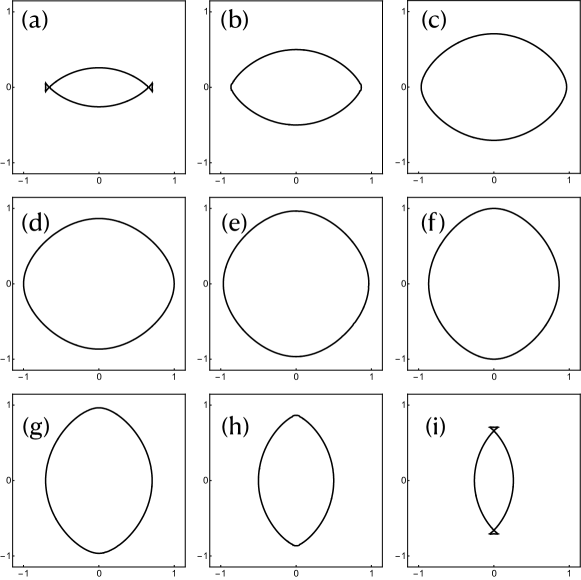
Here is the equation of amoeba’s contour, and and are deformations of Eq. S11 and Eq. S12, and is the resultant of the polynomials and with respect to the variable x. Fig S1 plots for different with fixed . Only when takes value outside spectrum, i.e. , can a central hole be found. As described in the main text ,one may also observe that when (symmetrically, ) , irregularity takes place at axis. In the following we shall make this observation valid.
Let’s take irregularity at x axis as an example and y axis can be treated similarly. Solve the equation ,
| (S16) |
Here we only need to deal with the first four roots since the remaining is just the inverse. Note that is always imaginary and is always real and regular. One can also check that appears as an irregular point, since it’s also a solution for . Thus, to make real, one need (we can always assume ). Then, recall that to make such an irregular point not isolated in the real plane, its Hessian matrix of second derivatives should have both positive and negative eigenvalues, and this gives the other side of the constraint. The Hessian matrix for reads as . Take both constraints and the proposition is proved.
S-2.2 Equal amplitude of wave function
Because amoeba’s contour determines the localization length (determined by equation ) of the wave function along a certain direction , it is able to get the corresponding curves of the localization length of the wave function along different directions through amoeba’s contour Eq S15, which is also the curve of the equal amplitude of the wave function.
| (S17) |
This curve is deemed concave if it exhibits negative and positive curvature along its path, so the transition point between a concave curve and a convex curve is the point at which zero curvature first appears in the path. Using the Hessian matrix to calculate the curvature of the curve, we can find that zero curvature exists in the region with .
S-2.3 Effect of weak non-Hermiticity
Let’s first recast some facts on wavefunction in the Hermitian lattice case in the language of amoeba. In Eq. S15 , let and one get
| (S18) |
The precise form of the function is not important. What matters here is that appears in the function as a whole due to symmetry, which we can also get from eq.S10. This implies that the contour should be a circle, whose radius can be read from eqS16 as . Thus, the wavefunction here is isotropic with localization length .
A few corollaries are ready in hand. First, comparing with the a real , a complex one with same strength tends to suppress the localization of wavefunction. Second, when x and y are not symmetric, i.e., the hoppings are different, the contour of amoeba shall take the form of an ellipse and so will the geometry of wavefunction. One may also note that the mix term shall rotate the orientation of this ellipse.
Next, we fix the bound state energy real () and show the result when one poses the non-Hermiticity to the lattice. In eq.S15, fix a direction by defining and treat as an implicit function of with parameters of , allowing one to expand it at
| (S19) |
Note that the odd powers of terms naturally vanish since it’s an even function. The negativity of the coefficient of the second order implies that in this case non-Hermiticity also suppresses the localization of the bound state. Further notice as a function of k is monotone in and and vanishes at minimal , so such suppression is not isotropic and do not influence localization at x axis, a fact which can also be retained from Eq. S16 and understood intuitively since non-Hermiticity is only imposed to y axis.
S-2.4 relationship of the argument of bound state energy and impurity
In the main text, we established the relationship between bound state energy and impurity near bloch saddle point via evaluating the integral with model ,i.e.
| (S20) |
Note that , the Complete elliptic integral of the first kind, has asymptotic expansion near 1 as ,and one can get
| (S21) |
Thus, the argument of bound state energy is linear with respect to the argument of impurity, i.e.
| (S22) |
S-3 Local Density of States
In this section, we will illustrate how the concavity and convexity of the wave function is reflected in LDOS by calculating LDOS. We consider a non-Hermitian system with an impurity at the origin. Through perturbation theory, we can know that when impurities are added, the Green’s function of the system can be calculated as,
| (S23) |
here represents the perturbed Green’s function, represents the unperturbed Green’s function with its entity at origin denoted as .
From Eq. 3 in the text, we can know that is proportional to the wave function of the bound state, and based on the previous discussion, we know that under the limit of weak impurity, the amoeba contour that determines the wave function has inversion symmetry about the origin. Therefore, our wave function should have inversion symmetry, so that our Green’s function is proportional to the square of the wave function. As a result, LDOS will inherit the concavity and convexity of the wave function.
S-4 Discussion on strong impurity case
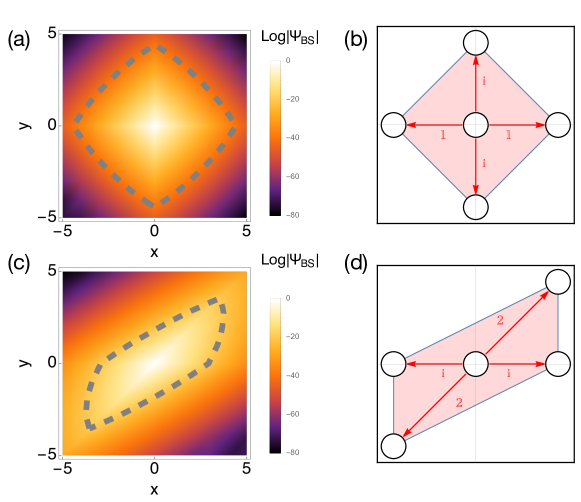
As the impurity strength increases, the shape of the bound state wave function progressively approximates a polygon and ultimately can be represented by a polytope known as the Newton Polytope, which is determined by the Bloch Hamiltonian. The Newton Polytope of a polynomial is defined as the convex hull of the set of exponent vectors of monomials within it. Physically, the Newton Polytope is analogous to the convex hull of the hopping graph, which represents all the hopping terms in the Hamiltonian, as illustrated in Fig S2(b) and (d).
As the impurity strength increases, the central hole of the amoeba expands and retreats to its spine, which is a dual representation of the system’s Newton Polytope. Since the shape of the wave function is dictated by its localization length—a dual of the amoeba’s contour, which encompasses the central hole, the wave function’s shape resembles that of the Newton Polytope.
In Fig. S2, we present the results for two examples of Hamiltonians. The first model incorporates the nearest hopping term, leading to a diamond-shaped Newton Polytope as illustrated in Fig. S2(b). The corresponding wavefunction is plotted in Fig. S2(a), exhibiting a diamond-like form. Conversely, the second model features a parallelogram-shaped Newton Polytope shown in Fig. S2(d), accompanied by its parallelogram-like wave function depicted in Fig. S2(c).
References
- [1] Passare, M. & Tsikh, A. Amoebas: their spines and their contours. Contemporary Mathematics 377, 275–288 (2005).
- [2] Gelfand, I., Kapranov, M. & Zelevinsky, A. Discriminants, Resultants, and Multidimensional Determinants (Birkhäuser Boston, 2013). URL https://books.google.nl/books?id=PC4AswEACAAJ.
- [3] Krasikov, V. A. A survey on computational aspects of polynomial amoebas. Mathematics in Computer Science 17, 16 (2023). URL https://doi.org/10.1007/s11786-023-00570-x.