Mastering truss structure optimization with tree search

Résumé

This study investigates the combined use of generative grammar rules and Monte Carlo Tree Search (MCTS) for optimizing truss structures. Our approach accommodates intermediate construction stages characteristic of progressive construction settings. We demonstrate the significant robustness and computational efficiency of our approach compared to alternative reinforcement learning frameworks from previous research activities, such as Q-learning or deep Q-learning. These advantages stem from the ability of MCTS to strategically navigate large state spaces, leveraging the upper confidence bound for trees formula to effectively balance exploitation-exploration trade-offs. We also emphasize the importance of early decision nodes in the search tree, reflecting design choices crucial for identifying the global optimum. Additionally, we show how MCTS dynamically adapts to complex and extensive state spaces without significantly affecting solution quality. While the focus of this paper is on truss optimization, our findings suggest MCTS as a powerful tool for addressing other increasingly complex engineering applications.

1 Introduction

Machine learning (ML) is impacting engineering applications, from structural health monitoring [1, 2] and predictive maintenance [3], to optimal flow control [4] and automation in construction [5]. Thanks to algorithmic advances and increased computational capabilities, there is a promise in enabling new approaches in computational design synthesis (CDS) — a multidisciplinary research field aimed at automating the generation of design solutions for complex engineering problems [6, 7, 8]. By integrating constraints related to the fabrication process, for instance through physics-based simulation, CDS could unlock the potential of additive manufacturing in various fields [9], e.g., concrete printing [10].

The effectiveness of traditional approaches to truss optimization, such as the ground-structure method [11, 12], has been established through decades of research. However, these methods suffer from high computational complexity and solution instability [13, 14]. Alternative strategies for discrete truss optimization rely on heuristic techniques, including genetic algorithms [15, 16, 17], particle swarm [18, 19], differential evolution [20], and simulated annealing [21]. Nevertheless, the applicability of these methods is similarly limited by their high computational burden and slow convergence as the size of the search space increases [14].

The search space of candidate solutions can be narrowed through generative design grammars [22], which facilitate the exploration of alternative designs within a coherent framework [23, 24]. These grammars are structured sets of rules that constrain the space of design configurations by accounting for mechanical information, such as the stability of static equilibrium. By integrating these rules within optimization procedures, it is therefore possible to explore incremental construction processes where the final design is reached through intermediate feasible configurations. The use of grammar-based approaches for truss topology generation and optimization has been proposed in [25], while their integration within heuristic approaches has been explored in [26, 27, 28, 29, 30].

Recently, the optimal truss design problem has been formalized as a Markov decision process (MDP) [31]. The solution to an MDP involves a series of choices, or actions, aimed at maximizing the long-term accumulation of rewards, which in this context measures the design objective. Viewing truss optimal design through the MDP lens, an action consists of adding or removing truss members, with the ultimate goal of optimizing a design objective, e.g., minimize the structural compliance. The final design thus emerges from a series of actions, possibly guided by grammar rules. This procedure is particularly suitable for truss structures, as it naturally accommodates discrete structural optimization, where adding a single member can significantly alter the functional objective of the design problem. Additionally, it can be extended to design optimization in additive manufacturing settings and continuum mechanics. The same methodology is similarly applicable to parametric optimization problems [32], including cases with stochastic control variables [33].

Reinforcement learning (RL) is the branch of ML that addresses MDPs through repeated and iterative evaluations of how a single action affects a certain objective [34]. Relevant instances of RL-based optimization in engineering include two-dimensional kinematic mechanisms [35] and the ground-structure of binary trusses [36]. The advantage of RL over heuristic methods lies in its flexibility in handling high-dimensional problems, as demonstrated in [37, 38, 39]. In [31], the MDP formalizing the optimal truss design has been solved using Q-learning [40], constraining the search space with the grammar rules proposed in [41]. In a separate work [42], the same authors have also addressed the challenges of large and continuous design spaces through deep Q-learning.

In this paper, we demonstrate how addressing optimal truss design problems with the Monte Carlo tree search (MCTS) algorithm [43, 44] can offer significant computational savings compared to both Q-learning and deep Q-learning. MCTS is the model-free RL algorithm behind the successes achieved by “AlphaGo” [45] and its successors [46, 47] in playing board games and video games. In science and engineering, MCTS has been used for various applications employing its single-player games version [48]. Notable instances include protein folding [49], materials design [50, 51], fluid-structure topology optimization [52], and the optimization of the dynamic characteristics of reinforced concrete structures [53].

For truss design, MCTS has been used in “AlphaTruss” [54] to achieve state-of-the-art performance while adhering to constraints on stress, displacement, and buckling levels. The same framework has been extended to handle continuous state-action spaces through either kernel regression [55] or soft actor-critic [56] — an off-policy RL algorithm. Despite the potential of using continuous descriptions of the design problem, the combination of RL and grammar rules proposed in [31, 42] remains highly competitive, as it enables constraining the design process with strong inductive biases reflecting engineering knowledge. Building on this insight, the novelty of our approach lies in the integration of MCTS with grammar rules to strategically navigate the solution space, allowing for significant computational gains compared to [31, 42], where Q-learning and deep Q-learning have been respectively adopted.

The effectiveness of the proposed approach lies in the MCTS capability to propagate information from the terminal nodes of the tree, which are associated with the final design performance, back to the ancestor nodes linked with the initial design states. This feedback mechanism allows for sequentially informing subsequent simulations, exploiting previously synthesized designs to enhance the decision-making process at initial branches and progressively refine the search towards optimal designs. Moreover, the probabilistic nature of MCTS enables the discovery of optimal design solutions by balancing the exploitation-exploration trade-off. This balance is achieved through a heuristic hyperparameter that tunes the Upper Confidence bound for Trees (UCT) formula, whose effect is investigated through a parametric analysis.

The remainder of the paper is organized as follows. Section 2 first states the optimization problem and provides an overview of the MDP setting, the grammar rules, and the MCTS algorithm. In Sec. 3, the computational procedure is assessed on a series of case studies. We provide both comparative results with respect to [31, 42], demonstrating superior design capabilities, and test our methodology on a progressive construction setup. Section 4 finally summarizes the obtained results and draws the conclusions.

2 Methodology

In this section, we describe the methodology characterizing our optimal truss design strategy. This includes the physics-based numerical model behind the design problem in Sec. 2.1, the MDP formalizing the design process in Sec. 2.2, the grammar rules for truss design synthesis in Sec. 2.3, the MCTS algorithm for optimal truss design formulated as an MDP in Sec. 2.4, and the UCT formula behind the selection policy in Sec. 2.5, before detailing their algorithmic integration in Sec. 2.6.

2.1 Optimal truss design problem

The design problem involves defining the truss geometry that optimizes a design objective under statically applied loading conditions. In the following, we consider minimizing the maximum absolute displacement experienced by the structure, although this is not a restrictive choice. This design setting, similar to the compliance minimization problem typical of topology optimization [13], has been retained for the purpose of comparison with [31, 42].

For the sake of generality, we set the design problem in the context of continuum elasticity, of which truss design is an immediate specialization. Specifically, we seek a set of $I$ subdomains $\{\Omega^{s}_{1},\ldots,\Omega^{s}_{I}\}$, each occupying a certain region of the design domain, whose union $\Omega=\bigcup^{I}_{i=1}\Omega^{s}_{i}$ minimizes the displacement experienced by the structure to the greatest extent, as follows:

$$\bar{\Omega}=\bigcup^{I}_{i=1}\bar{\Omega}^{s}_{i}=\operatorname*{arg\,min}_{\Omega=\bigcup^{I}_{i=1}\Omega^{s}_{i}}\lVert\mathbf{u}(\mathbf{x})\rVert_{\infty},\quad\text{with }\mathbf{x}\in\Omega,$$ (1)

where $\mathbf{u}$ is the displacement field, $\mathbf{x}$ are the spatial coordinates, and $\lVert\mathbf{u}\rVert_{\infty}$ is the infinity norm of $\mathbf{u}$, defined as $\lVert\mathbf{a}\rVert_{\infty}=\operatorname*{max}_{m}\lvert a_{m}\rvert$, with $a_{m}$, $m=1,\ldots,M$, being the $m$-th entry of $\mathbf{a}\in\mathbb{R}^{M}$. Problem (1) is subjected to the following constraints, $\forall\Omega=\bigcup^{I}_{i=1}\Omega^{s}_{i}$:

$$\nabla\cdot\bm{\sigma}+\mathbf{b}=0$$ equilibrium, (2a)

$$\bm{\sigma}=\mathbf{E}\bm{\epsilon}$$ linear elastic constitutive law, (2b)

$$\bm{\epsilon}=\frac{\nabla\mathbf{u}+\nabla\mathbf{u}^{\top}}{2}$$ linear kinematic compatibility, (2c)

ensuring the static elasticity condition. Herein, $\bm{\sigma}$ is the stress field; $\bm{\epsilon}$ is the strain field; $\mathbf{b}$ is the vector of body forces; $\mathbf{E}$ is the elasticity tensor; $(\nabla\cdot)$ is the divergence operator; and $(\nabla)$ is the gradient operator.

Moreover, problem (2) needs to be equipped with the following set of boundary conditions (BCs):

$$\mathbf{u}=\mathbf{u}_{g}, \text{on }\partial\Omega_{g}=\bigcup^{I}_{i=1}\partial{\Omega_{g}^{s}}_{i}\qquad\leavevmode\nobreak\ \text{Dirichlet BC,}$$ (3a)

$$\bm{\sigma}\cdot\mathbf{n}=\mathbf{f}, \text{on }\partial\Omega_{h}=\bigcup^{I}_{i=1}\partial{\Omega^{s}_{h}}_{i}\qquad\text{Neumann BC,}$$ (3b)

where, $\partial\Omega_{g}$ and $\partial\Omega_{h}$ are the Dirichlet and Neumann boundaries, respectively; $\mathbf{u}_{g}$ is the assigned displacement field on $\partial\Omega_{g}$; $\mathbf{f}$ is the vector of surface tractions acting on $\partial\Omega_{h}$; and $\mathbf{n}$ is the outward unit vector normal to $\partial\Omega_{h}$. It is worth highlighting that this framework can be generalized to include non-linear constitutive behaviors — an extension that will be explored in future works.

Equation (1) can be easily adapted for planar trusses by introducing a finite element (FE) discretization to solve problem (2), defining each subdomain $\Omega^{s}_{i}$, $i=1,\ldots,I$, to be a truss element, with the union set operator representing the connections made through hinges. Accordingly, the optimization problem is reformulated as:

$$\min_{\Omega=\bigcup^{I}_{i=1}\Omega^{s}_{i}} \ \ \lVert\mathbf{U}(\Omega)\rVert_{\infty},\leavevmode\nobreak\ \leavevmode\nobreak\ \text{with }\Omega^{s}_{i}\text{ a truss FE,}$$ (4a)

$$\text{subject to}: \ \ \mathbf{K}\mathbf{U}=\mathbf{F},\quad\leavevmode\nobreak\ \text{in }\Omega=\bigcup^{I}_{i=1}\Omega_{i},$$ (4b)

$$\ \ \mathbf{U}=\mathbf{U}_{0},\leavevmode\nobreak\ \quad\text{on }\partial\Omega_{g}=\bigcup^{I}_{i=1}\partial{\Omega_{g}^{s}}_{i},$$ (4c)

$$\ \ V\leq V^{\text{max}},\text{ with }V=\sum_{i=1}^{I}A_{i}L_{i},$$ (4d)

where $\mathbf{U}$ is the vector of nodal displacements; $\mathbf{K}$ is the stiffness matrix; $\mathbf{F}$ is the vector of forces induced by the external loadings; $\mathbf{U}_{0}$ is the vector of nodal displacements enforced on $\partial\Omega_{g}$; $A_{i}$ and $L_{i}$ are the cross-sectional area and the length of the $i$-th truss element $\Omega^{s}_{i}$, respectively; and $V^{\text{max}}$ is a prescribed threshold on the maximum allowed volume of the truss lattice. For further details on the FE method, the reader may refer to [57].

2.2 MDP framework for sequential decision problems

In a decision-making setting, an agent must choose from a set of possible actions, each potentially leading to uncertain effects on the state of the system. The decision-making process aims to maximize, at least on average, the numerical utilities assigned to each possible action outcome. This involves considering both the probabilities of various outcomes and our preferences among them.

In sequential decision problems, the agent’s utility is influenced by a sequence of decisions. MDPs provide a framework for describing these problems in fully observable, stochastic environments with Markov transition models and additive rewards [58]. Formally, an MDP is a $4$-tuple $\langle\mathcal{S},\mathcal{A},\mathcal{P},\mathcal{R}\rangle$, comprising a space of states $\mathcal{S}$ that the system can assume, a space of actions $\mathcal{A}$ that can be taken, a Markov transition model $\mathcal{P}$, and a space of rewards $\mathcal{R}$. The characterization of these quantities for truss optimization purposes is detailed below, after discussing their roles in MDPs.

We consider a time discretization of a planning horizon $(0,T)$ using non-dimensional time steps $t=0,\ldots,T$, and denote the system state at time $t$ as $s_{t}\in\mathcal{S}$, which is the realization of the random variable $S_{t}\sim p(s_{t})$, with $p(s_{t})$ being the probability distribution encoding the relative likelihood that $S_{t}=s_{t}$. Moreover, we denote the control input at time $t$ as $a_{t}\in\mathcal{A}$. The transition model $\mathcal{P}:\mathcal{S}\times\mathcal{S}\times\mathcal{A}\mapsto[0,1]$ encodes the probability of reaching any state $s_{t+1}$ at time $t+1$, given the current state $s_{t}$ and an action $a_{t}$, i.e., $p(s_{t+1}|s_{t},a_{t})\in\mathcal{P}$. The reward $R_{t}\sim p(r_{t})$, with $r_{t}\in\mathcal{R}$, quantifies the value associated with each possible set $\{s_{t},a_{t},s_{t+1}\}$.

We define a control policy $\pi:\mathcal{S}\mapsto\mathcal{A}$ as the mapping from any system state to the space of actions. The goal is to find the optimal control policy $\pi^{*}(S_{t})$ that provides the optimal action $a^{*}_{t}$ for each possible state $s_{t}$. The optimal policy $\pi^{*}(S_{t})$ is learned by identifying the action $a^{*}_{t}$ that maximizes the expected utility over $(0,T)$. The problem of finding the optimal control policy is inherently stochastic. Consequently, the associated objective function is additive and relies on expectations [59]. This is typically expressed as the total expected discounted reward over $(0,T)$.

The sequential decision problem can be viewed from the perspective of an agent-environment interaction, as depicted in Fig. 1. In this view, the agent perceives the environment and aims to maximize the long-term accumulation of rewards by choosing an action $a_{t}$ that influences the environment at time $t+1$. The environment interacts with the agent by defining the evolution of the system state, and providing a reward $r_{t}$ for taking $a_{t}$ and moving to $s_{t+1}$.

Figure 1: Schematic agent-environment interaction.

One way to characterize an MDP is to consider the expected utility associated with a policy $\pi(S_{t})$ when starting in any state $s_{t}$ and following $\pi(S_{t})$ thereafter. To this aim, the state-value function $V^{\pi}(S_{t}):\mathcal{S}\mapsto\mathbb{R}$ quantifies, for every state $s_{t}$, the total expected reward an agent can accumulate starting in $s_{t}$ and following policy $\pi(S_{t})$. In contrast, the action-value function, $Q^{\pi}(S_{t},a_{t}):\mathcal{S}\times\mathcal{A}\mapsto\mathbb{R}$ reflects the expected accumulated reward starting from $s_{t}$, taking action $a_{t}$, and then following policy $\pi(S_{t})$. In both cases, the probability of each reaching any state $s_{t+1}$ is estimated using transition probabilities $p(s_{t+1}|s_{t},a_{t})$.

For our purposes of optimal truss design, we refer to a grid-world environment with a predefined number of nodes on which possible truss layouts can be defined. The reward function shaping $\mathcal{R}$ could account for local design objectives, such as the displacement at a prescribed node, or global performance indicators, such as the maximum absolute displacement, stress level, or strain energy. As previously commented, we monitor the maximum absolute displacement experienced by the structure. The state space $\mathcal{S}$ could potentially include any feasible truss layout resulting from progressive construction processes. Accordingly, the space of actions $\mathcal{A}$ could account for any possible modification of a given layout. In this scenario, the sizes of $\mathcal{S}$ and $\mathcal{A}$ increase significantly, even considering a reasonably small design domain. For this reason, explicitly modeling the Markov transition model $\mathcal{P}$ is not feasible.

The availability of a transition model for an MDP influences the selection of appropriate solution algorithms. Dynamic programming algorithms, for instance, require explicit transition probabilities. In situations where representing the transition model becomes challenging, a simulator is often employed to implicitly model the MDP dynamics. This is typical in episodic RL, where an environment simulator is queried with control actions to sample environment trajectories of the underlying transition model. Exemplary algorithms include Q-learning, as seen in [31, 42], and MCTS, both of which approximate the action-value function and use this estimate as a proxy for the optimal control policy. In our truss design problem, optimal planning is achieved via simulated experience provided by the FE model in Eq. (4b), which can be queried to produce a sample transition given a state and an action.

2.3 Grammar rules for truss design synthesis

To introduce the graph grammar rules that we employ to guide the process of optimal design synthesis, we refer to a starting seed configuration $s_{0}$, defined by deploying a few bars to create a statically determinate truss structure. This initial configuration must be modified through a series of actions selected by an agent. Every time an allowed action is enacted on the current state $s_{t}$, a new configuration $s_{t+1}$ is generated (see Fig. 2). The process continues until reaching a state $s_{T}$, characterized by a terminal condition, such as achieving the maximum allowed volume $V^{\text{max}}$ of the truss members .

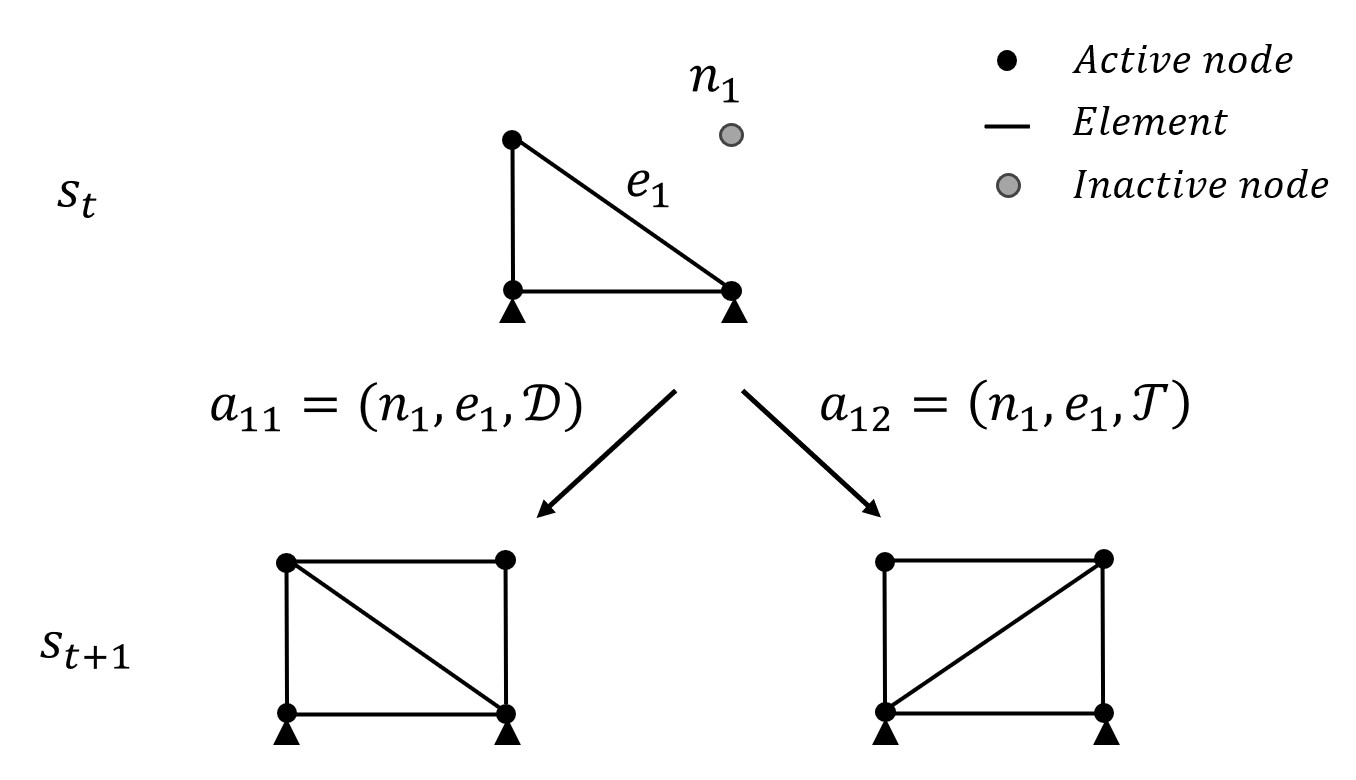
Figure 2: Exemplary actions following operators $\mathcal{D}$ and $\mathcal{T}$. The current configuration $s_{t}$ (top) is modified either through action $a_{1}$ (bottom left) following the $\mathcal{D}$ operator or through action $a_{2}$ (bottom right) following the $\mathcal{T}$ operator, resulting in a new configuration $s_{t+1}$. In both cases, the selected truss element is $e_{1}$, and the chosen inactive node is $n_{1}$.

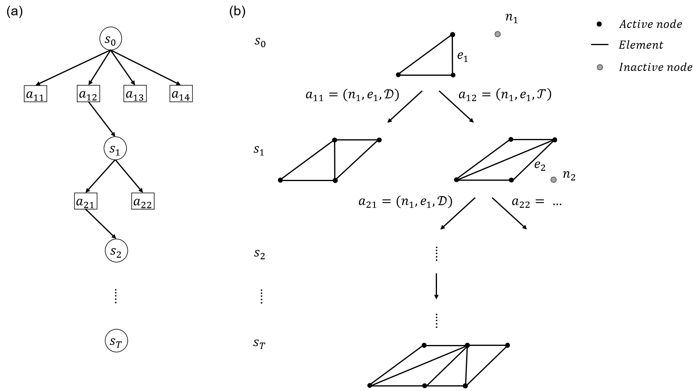
Figure 3: Exemplary use of grammar rules for optimal truss design, formalized as a Markov decision process solved through Monte Carlo tree search: (a) search tree, and (b) corresponding truss design synthesis.

To identify the allowable actions, we use the same grammar rules as those used in [41, 31, 42]. Starting from an isostatic seed configuration, these rules constrain the space of design configurations by allowing only truss elements resulting in triangular forms to be added to the current configuration, thereby ensuring statically determinate configurations. Given any current configuration $s_{t}$, an allowed action is characterized by a sequence of three operations:

1. Choosing a node among those not reached by any already placed truss element. We term these nodes as inactive, to distinguish them from the previously selected active nodes.

2. Selecting a truss element already in place.

3. Applying a legal operator based on the position of the chosen node with respect to the selected element. The legal operators are either “$\mathcal{D}$” or “$\mathcal{T}$”, see also Fig. 2. A $\mathcal{D}$ operator adds the new node and links it to the current configuration without removals, while a $\mathcal{T}$ operator also removes the selected element before connecting the new node. In both cases, the connections to the new node are generated ensuring no intersection with existing elements.

2.4 Monte Carlo tree search

The MCTS algorithm is a model-free RL method for decision-time planning [34]. The algorithm relies on two fundamental principles: ($i$) approximating the action-values through random sampling of simulated environment trajectories, and ($ii$) using these estimates to inform the sequential exploration of the search space, progressively refining the search toward more highly-rewarding trajectories.

In the context of optimal truss design, formulated as a sequential decision-making problem, MCTS incrementally constructs a search tree where each node represents a specific design configuration, and the connections to child nodes correspond to potential state transitions triggered by allowed actions, see Fig. 3. MCTS performs many iterations to incrementally improve a tree policy derived from value estimates of each state–action pair. The algorithm is executed after encountering each new state to select an action for that state. An execution involves many rollouts, each simulating a trajectory starting from the current state $s_{t}$ and evolving the structure to a terminal state $s_{T}$. Actions outside the tree are selected following a random policy guided by grammar rules, known as the rollout policy. For each rollout reaching a terminal state, a trial design is synthesized to assess the value of the design objective. After simulating a collection of sample environment-interaction trajectories, the value of each state–action pair departing from $s_{t}$ are derived from Monte Carlo estimates of the average return gained from that pair. In this way, the rollout policy allows for improving the tree policy, making the preferable state–action pairs more likely to be chosen in the future. Only nodes representing states that look promising, based on the results of the simulated trajectories, are added to incrementally extend the tree. In other words, MCTS focuses multiple simulations starting at $s_{t}$ by extending the initial common portions of previously simulated high-return trajectories, balancing exploitation and exploration. This construction of the tree is termed the training phase. Each time $s_{T}$ is reached, an episode is completed. The number of episodes is determined by the available computational budget. As the number of episodes increases, the tree expands, and the precision of the estimated action-values improves.

Each round of MCTS comprises four steps [34]:

1. Selection: Starting from the root node, the tree policy identifies a path to a leaf node according to the estimated values of the state–action pairs.

2. Expansion: If the selected leaf node allows for expanding the tree, one or more child nodes are created to reflect possible future, yet unexplored actions.

3. Simulation: From the selected node, a Monte Carlo trial of environment interaction is simulated using the rollout policy.

4. Backpropagation: The returns generated by a set of simulations are used to update the value estimates of the state–action pairs traversed by the tree policy.

MCTS continues executing these four steps for each episode. The tree policy expands the tree through selection and expansion, and the rollout policy simulates outcomes from the current tree structure, which are then backed up to update node statistics to inform future decisions. After completing the available episodes, a deterministic policy is derived from the estimated values following each particular state-action pair.

The advantages of MCTS stem from its online, incremental, sample-based value estimation and policy improvement. MCTS is particularly adept at managing environments where rewards are not immediate, as it effectively explores broad search spaces despite the minimal feedback. This makes MCTS especially suitable for progressive construction settings, where the final design requirements often differ from those of intermediate structural states. Intermediate construction stages typically involve sustaining self-load only, while different combinations of dead and live loads are usually experienced during operations. This capability stems from the backpropagation step, which allows information related to $s_{T}$ to be transferred to the early nodes of the tree. In contrast, bootstrapping methods like Q-learning may require a longer training phase to equivalently back-propagate information, as will be demonstrated in Sec. 3. Further advantages of MCTS include: ($i$) accumulating experience by sampling environment trajectories, without requiring domain-specific knowledge to be effective; ($ii$) incrementally growing a lookup table to store a partial action-value function for the state–action pairs yielding highly-rewarding trajectories, without needing to approximate a global action-value function; ($iii$) updating the search tree in real-time whenever the outcome of a simulation becomes available, in contrast, e.g., with minimax’s iterative deepening; and ($iv$) focusing on promising paths thanks to the selective process, leading to an asymmetric tree that prioritizes more valuable decisions. This last aspect not only enhances the algorithm’s efficiency but can also offer insights into the domain itself by analyzing the tree’s structure for patterns of successful courses of action.

2.5 Upper Confidence bounds for Trees

The UCT formula is a widely used selection policy in MCTS because of its capability to balance exploitation and exploration. Here, we employ a modified UCT formula compared to that proposed in [44], which includes an $\alpha$ parameter to scale the relative weights of the exploitation and exploration terms, as follows:

$$\text{UCT}_{j}=(1-\alpha)\frac{v^{\Sigma}_{j}}{n_{j}}+\alpha\sqrt{\frac{2\log\sum_{l}n_{l}}{n_{j}}},$$ (5)

providing the UCT score of the $j$-th child node of $s_{t}$. Herein: $v^{\Sigma}_{j}$ is the Monte Carlo estimate of the total return gained by passing through the $j$-th child node at the end of the training episode; $n_{j}$ is the number of simulations passing through the $j$-th child node; $\sum_{l}n_{l}$ is the total number of simulations traversing the children of $s_{t}$; and $\alpha$ is a parameter to balance exploitation (average reward for the $j$-th child node) and exploration (encourages exploring nodes that have not been visited as frequently as their siblings), respectively encoded in the first and second terms. It is worth highlighting that both $v_{j}$ and $n_{j}$ are updated at each training step.

2.6 Algorithmic description

The algorithmic description of the optimal truss design strategy using the proposed MCTS approach is detailed in algorithm 1. It begins by initializing the root node with a seed configuration and iteratively explores potential truss configurations through a sequence of selection, expansion, simulation, and backpropagation phases. During each episode, the algorithm selects child nodes based on the UCT formula, generates and evaluates new child nodes from possible actions, simulates random child nodes to explore the design space, and backpropagates the computed rewards to update the policy.

input: number of episodes $N_{e}$
              parametrization of the physics-based model
              grid design domain
              seed configuration
              grammar rules for truss design synthesis
              exploration parameter $\alpha$

1:initialize root node for the seed configuration

2:for $N_{e}$ do

3:     $t=0$

4:     set root node for $s_{t=0}$ (seed configuration)

5:$\triangleright$ selection

6:     while $t<T$ and $s_{t}$ previously explored do

7:         select $s_{t+1}$ via UCT formula

8:         $t\leftarrow t+1$      

9:$\triangleright$ expansion

10:     if $t<T$ and $s_{t}$ not previously explored then

11:         for states $s_{t+1}$ from allowed actions $a_{t}$ do

12:              solve static equilibrium for $s_{t+1}$

13:              compute design objective $\lVert\mathbf{U}(\Omega)\rVert_{\infty}$          

14:         $t\leftarrow t+1$      

15:$\triangleright$ simulation

16:     while $t<T$ do

17:         select a random child $s_{t+1}$

18:         if $s_{t+1}$ not previously explored then

19:              solve static equilibrium for $s_{t+1}$

20:              compute design objective $\lVert\mathbf{U}(\Omega)\rVert_{\infty}$          

21:         $t\leftarrow t+1$      

22:$\triangleright$ backpropogation

23:     compute reward $r_{T}$ from terminal state $s_{T}$

24:     while $t>0$ do

25:         append $r_{T}$ to $s_{t}$ rewards list

26:         $s_{t}$ visit count += 1

27:         $t\leftarrow t-1$      

28:return deterministic control policy $\pi\approx\pi^{*}$

Algorithm 1 Monte Carlo tree search for optimal truss design

3 Results

In this section, we assess the proposed MCTS framework on different truss optimization problems. First, we adopt six case studies from [31, 42], each featuring different domain and boundary conditions, to directly compare the achieved performance. Then, we consider an additional case study to demonstrate the applicability of the proposed procedure for progressive construction purposes. While in the former case studies the seed configurations fully cover the available design domain, in the latter one we allow the seed configuration to expand — mimicking an additive construction process — until reaching a terminal node at the far end of the domain.

The experiments have have been implemented in Python using the Spyder scientific environment. All computations have been carried out on a PC featuring an AMD Ryzen^TM 9 5950X CPU @ 3.4 GHz and 128 GB RAM.

3.1 Truss optimization

In the following, we present the results achieved for the six case studies adapted from [31, 42], providing comparative insights for each scenario. All case studies deal with planar trusses, with truss elements featuring dimensionless Young’s modulus $E=10^{3}$ and cross-sectional area $A=1$. The dimensionless value of the applied forces is equal to $f_{x}=f_{y}=10$, as per [31, 42]. The recorded displacement refers to the maximum absolute displacement experienced by the structure.

Each row of Tab. 1 characterizes a case study in terms of the size of the design domain, the number of decision times or planning horizon $T$, and the volume threshold $V^{\text{max}}$. For all case studies, the specified design domain, structural seed configuration, externally applied force(s), and boundary conditions are shown under the corresponding $s_{0}$ label in Fig. 4. The final optimal configuration $s_{T}$, identified through a brute-force exhaustive search approach, is illustrated under the $s_{T}$ label.

Table 1: Truss optimization - Problems settings description.

	Domain size	Decision times $T$	$V^{\text{max}}$ threshold
Case 1	$4\times 3$	$2$	$160$
Case 2	$5\times 3$	$3$	$240$
Case 3	$5\times 5$	$3$	$225$
Case 4	$5\times 9$	$3$	$305$
Case 5	$5\times 5$	$4$	$480$
Case 6	$7\times 7$	$4$	$350$

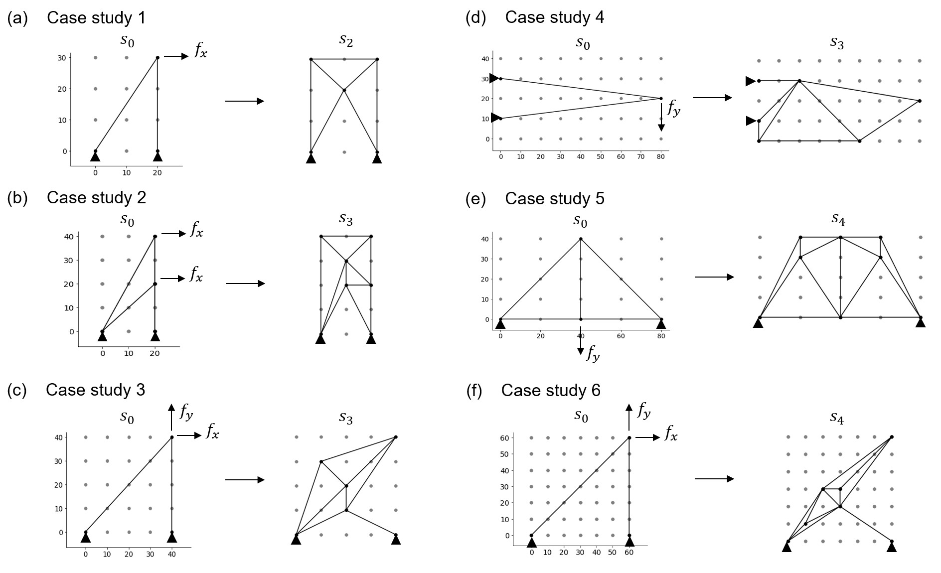
Figure 4: Truss optimization - Case studies adapted from [42]: summary of each design domain, seed configuration $s_{0}$, and target optimal design $s_{T}$ identified through a brute-force exhaustive search.

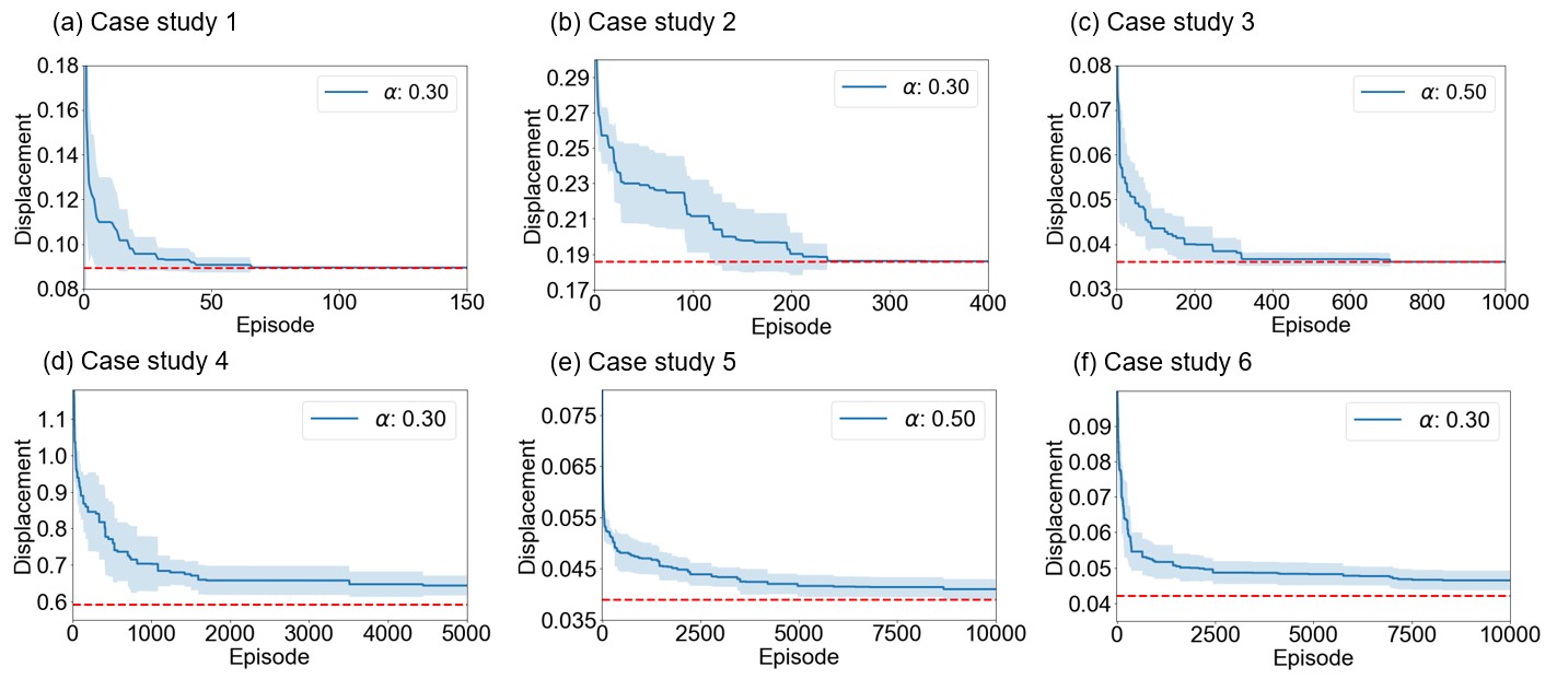
Figure 5: Truss optimization - Design objective evolution during training for case studies 1-6: average value (solid blue line) and one standard deviation credibility interval (shaded blue area) over 10 runs, and target global minimum (dashed red line).

For each case study, Fig. 5 shows the evolution of the design objective, i.e., the maximum absolute displacement experienced by the structure, as the number of episodes increases. Results are reported in terms of average displacement (solid blue line) and one standard deviation credibility interval (dashed blue area), over 10 independent training runs. Each run utilizes MCTS for a predefined number of episodes. In practice, the number of episodes is set after an initial long training run in which we assess the number of episodes required to achieve convergence — which typically depends on the complexity of the case study. After each training run, the best configuration is saved to subsequently compute the relevant statistics. The attained displacement values are compared with those associated with the global minima (red dashed lines), representing the optimal design configurations in Fig. 4.

Table 2: Truss optimization - Results averaged over 10 training runs for case studies 1-6, in terms of: optimal design objective $\lVert\mathbf{U}(\overline{\Omega})\rVert_{\infty}$, ratio of the optimal design objective to the displacement achieved by the learned policy in percentage terms (objective ratio), percentile score relative to the exhaustive search space (percentile score), number of finite element evaluations required to achieve a near-optimal or optimal policy, and relative speed-up compared to [42].

	$\lVert\mathbf{U}(\overline{\Omega})\rVert_{\infty}$	Objective	Percentile	FE runs	FE runs vs [42]
		ratio	score
Case 1	$0.0895$	$100\%$	$100\%$	$106$	$-74.70\%$
Case 2	$0.1895$	$100\%$	$100\%$	$517$	$-76.27\%$
Case 3	$0.0361$	$100\%$	$100\%$	$966$	$-56.51\%$
Case 4	$0.5916$	$91.91\%$	$99.90\%$	$1672$	$-70.85\%$
Case 5	$0.0390$	$95.23\%$	$99.99\%$	$9739$	$-70.74\%$
Case 6	$0.0420$	$90.44\%$	$99.98\%$	$7931$	$-31.25\%$

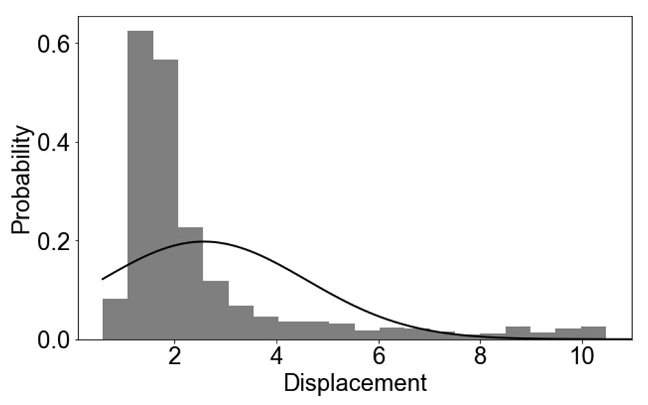
Figure 6: Truss optimization - Case study 4: design objective distribution over the population of designs synthesized from an exhaustive search of the configuration space.

The heuristic $\alpha$ parameter in Eq. (5) controls the balance of exploitation and exploration. The $\alpha$ values employed for the six case studies are overlaid on each learning curve in Fig. 5. Since an optimal value for this parameter is not known a-priori, this is set using a rule of thumb derived through a parametric analysis, as explained in the following section for case study 4.

A quantitative assessment of the optimization performance for each case study is summarized in Tab. 2. Results are reported in terms of the optimal design objective ($\lVert\mathbf{U}(\overline{\Omega})\rVert_{\infty}$), the ratio of the optimal design objective to the displacement achieved by the learned policy in percentage terms (objective ratio), and the percentile score relative to the exhaustive search space (percentile score). To clarify, a percentile score of $100\%$ corresponds to reaching the global optimum. A lower score, such as $99\%$, means that the design objective achieved with the final design $s_{T}$ synthesized from the learned optimal policy is lower than the displacement computed for $99\%$ of all the possible configurations explored through an exhaustive search. An exemplary distribution of the design objective over the population of designs synthesized from an exhaustive search of the configuration space is reported in Fig. 6 for case study 4. Interestingly, the distributions obtained for the other case studies also reveal a lognormal-like shape, although not shown here for the sake of space. While the objective ratio indicator offers a dimensionless measure of how close the achieved design is to the global optimum solution in terms of performance, the percentile score quantifies the capability of MCTS to navigate the search space to find a design solution close to the optimal one. Both performance indicators are computed by averaging over 10 training runs. Additionally, we report the number of FE evaluations required to achieve a near-optimal or optimal policy, also averaged over 10 training runs, and indicate the percentage savings in the number of FE evaluations compared to those needed by the deep Q-learning strategy from [42].

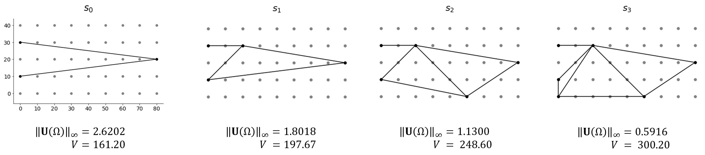
Figure 7: Truss optimization - Case study 4: sequence of design configurations from the target optimal policy, identified through a brute-force exhaustive search, with details about the design objective value and the volume of the truss lattice.

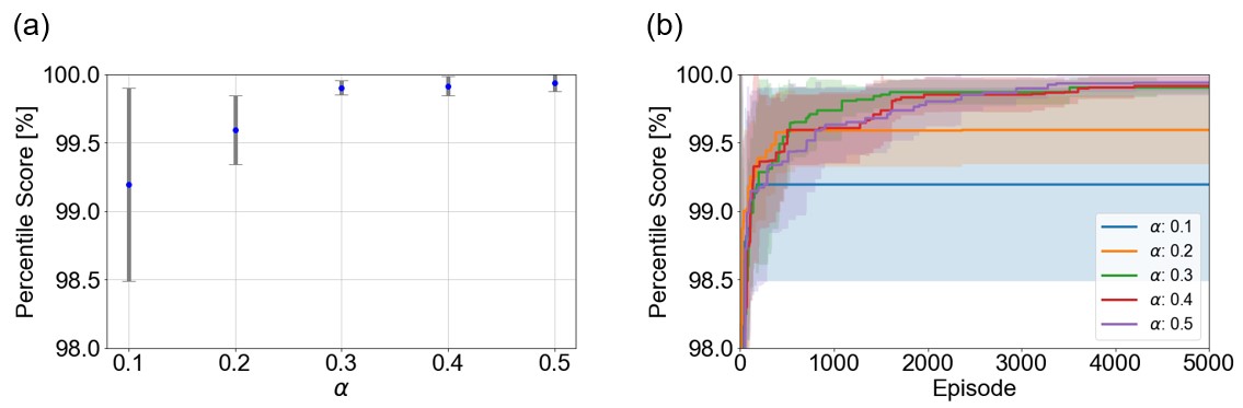
Figure 8: Truss optimization - Case study 4: impact of varying the $\alpha$ parameter on the attained value of the percentile score indicator. For each value of $\alpha$, results are reported in terms of (a) the percentile score relative to the exhaustive search space and its one standard deviation credibility interval, averaged over 10 training runs, and (b) the evolution of the percentile score and its credibility interval as the number of episodes increases, averaged over 10 training runs.

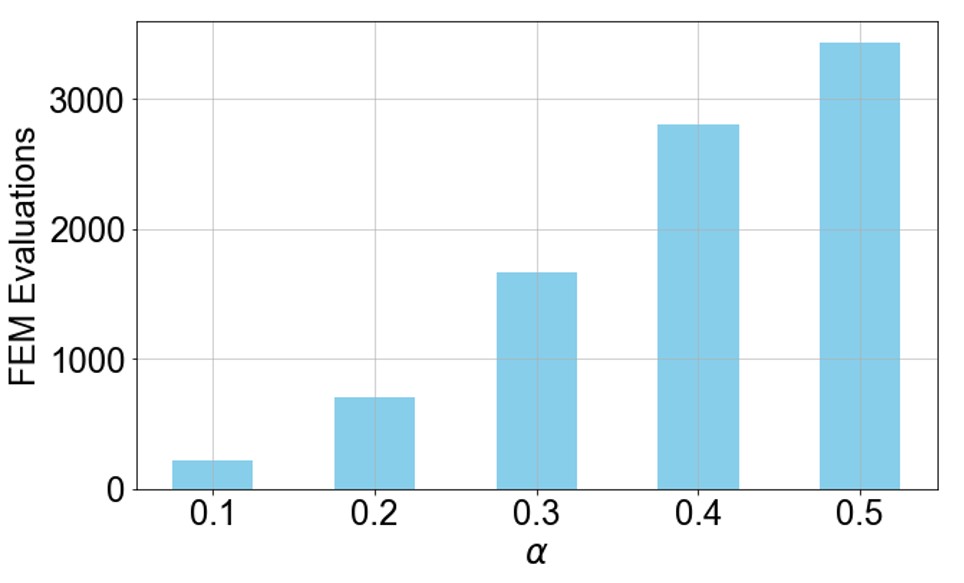
Figure 9: Truss optimization - Case study 4: number of finite element evaluations required to achieve a near-optimal design policy for varying values of the $\alpha$ parameter.

3.2 Case study 4 — detailed analysis

In this section, we provide a detailed analysis for case study 4. This case study is chosen as it is the only one where the optimal result found by our algorithm differs from that reported in [42], exhibiting a further improvement in the design objective. Figure 7 illustrates the sequence of structural configurations synthesized from the exhaustive search optimal policy. For each decision time, we report the corresponding value of design objective and volume of the truss lattice below the synthesized configuration $s_{t}$.

Figure 8 summarizes the impact of varying the $\alpha$ parameter on the attained percentile score, to provide insights into the selection of an appropriate value. Specifically, Fig. 8(a) displays the percentile score relative to the exhaustive search space for the different $\alpha$ values, averaged over 10 training runs. Figure 8(b) shows how the percentile score evolves as the number of episodes increases, providing insights into the effect of $\alpha$ on the convergence of MCTS. To compare the achieved performance for varying values of $\alpha$ with the associated computational burden, Fig. 9 shows the number of FE evaluations required to achieve a near-optimal design policy, highlighting an almost linear trend in the number of FE evaluations as $\alpha$ increases. Therefore, we deem $\alpha=0.3$ to be an adequate exploitation-exploration trade-off, resulting in a $99.90\%$ average percentile score across the 10 training runs, which is close to the percentile score for $\alpha=0.4$ and $\alpha=0.5$, while requiring only 1672 FE evaluations — a reduction of $70.85\%$ compared to [42]. The attained ratio of the optimal design objective to the displacement achieved by the learned policy is $91.91\%$ (see Tab. 2).

3.3 Progressive construction

In this section, we showcase the potential of the proposed MCTS strategy in guiding the progressive construction of a truss cantilever beam. Unlike in the previous case studies, here we allow the seed configuration to progressively grow until reaching a terminal node at the far end of the domain. Therefore, the agent must account for the intermediate construction stages per se, not just as necessary steps to reach the final configuration. Another difference compared to the previous case studies is that instead of considering a fixed external load, the structure is subjected to self-weight (unit dimensionless density), modifying the loading configuration at each stage. However, since the design process aims to maximize the performance of the final configuration, the chosen design objective is the displacement at a prescribed node, i.e., the terminal node. Although we did not set a limit on the maximum number of states, the agent must strike a balance between achieving higher structural stiffness by adding additional members and the weight these extra elements bring.

Figure 10: Progressive construction - Sequence of design configurations from the target optimal policy.

Figure 11: Progressive construction - Design objective evolution during training: average value (solid blue line) and one standard deviation credibility interval (shaded blue area) over 10 runs, and target global minimum (dashed red line).

Figure 10 illustrates the sequence of design configurations, from $s_{0}$ to $s_{7}$, synthesized from an exhaustive search stopped after reaching a state space made of $10,000,000$ possible configurations. To prevent trivial configurations and to force the algorithm to explore more detailed designs, an additional constraint on the maximum length of the individual elements is introduced to the optimization problem (4). After 10 training runs, using $\alpha=0.3$, the optimal configuration is synthesized $100\%$ of the time, requiring an average of 507 FE evaluations per training run, and yielding an optimal displacement of $20.861$. Thus, MCTS finds the optimal configuration by focusing only on the subset of most promising solutions, featuring more elements near the clamped side than in the vicinity of the free end (see $s_{7}$ in Fig. 10). Also, refer to Fig. 11 for the evolution of the attained design objective as the number of episodes increases during training.

This case study exemplifies the advantages of MCTS over Q-learning approaches to optimal design synthesis in problems with large state spaces. In these situations, Q-learning struggles because it requires a Q-table that stores values for every possible state-action pair, leading to exponential growth in memory and computational needs as the number of states increases. This makes it impractical for environments with a vast number of states due to the memory requirements and slow convergence caused by the need to sample each state-action pair sufficiently. In contrast, MCTS dynamically builds a decision tree based on the most promising moves explored through simulation, focusing computational resources on more relevant parts of the search space. This selective exploration helps MCTS manage larger state spaces more efficiently than Q-learning, making it a better fit for problems where direct enumeration of all state-action pairs is infeasible.

3.4 Discussion

In all six case studies adopted for comparison with [42], the proposed MCTS framework has been capable of synthesizing a near-optimal solution with a markedly lower number of FE evaluations. Case study 2 has shown the greatest reduction, requiring $76\%$ fewer evaluations compared to [42]. All examples have achieved a final percentile score greater than $99.9\%$ when compared with all candidate solutions found in the exhaustive search. In case studies 1, 2, and 3, the global optimal solution has been synthesized $100\%$ of the time. However, this was not the case for case studies 4, 5, and 6.

As seen in Tab. 2, case study 4 has the lowest percentile score. A significant factor contributing to this result is the large number of nodes present in the first layer of the decision tree. Although case study 4 has a smaller exhaustive search space compared to case study 5, it exhibits a considerably larger branching factor at the initial layer, with 94 child nodes as opposed to 42 in case study 5. This increased number of initial options introduces a greater degree of complexity, which can impede the algorithm’s convergence rate. Another major reason for this is that the optimal solution is located in a section of the tree crowded with numerous lower-quality configurations. However, the UCT formula (5) favors exploitation of areas of the tree that yield on average good results. Consequently, the procedure tends to overlook tree branches that potentially lead to the global optimum, in favor of branches that yield consistently good configurations. The rationale is that tree areas yielding, on average, better solutions typically also contain the best configurations. However, this is not necessarily true for every problem, and it is not true for case study 4. Even when reaching the global optimum is not precluded, this limitation of the UCT formula may slow the convergence to the optimum. To address these drawbacks, the UCT equation could be modified to account for the standard deviation and the maximum value of the reward obtained from traversing the branch of child nodes, similarly to [48, 60], as follows:

$$\text{UCT}^{\text{new}}_{j}=(1-\alpha)\left[\frac{(1-\beta)v^{\Sigma}_{j}}{n_{j}}+\beta v^{\text{best}}_{j}\right]+\alpha\sqrt{\frac{2\log\sum_{l}n_{l}}{n_{j}}+\text{var}(v_{j})},$$ (6)

where, $v^{\text{best}}_{j}$ and $\text{var}(v_{j})$ are the maximum value and the variance of the reward gained by passing through the $j$-th child node, respectively; while $\beta$ is a hyperparameter to balance the exploitation between tree areas consistently yielding good results and areas containing the best-seen state. This modified selection policy is less likely to be unfairly biased towards nodes with fewer children, while promoting increased exploration.

In the following, we provide a detailed analysis to investigate the effects of varying the heuristic $\alpha$ parameter, which controls the balance between exploitation and exploration in the UCT formula (5). From Fig. 8(b), we observe that for both $\alpha=0.1$ and $\alpha=0.2$, MCTS converges early on local minima. This occurs because the first term in the UCT formula dominates the second term during training, preventing sufficient exploration of child nodes in the tree. While increasing the value of $\alpha$ mitigates this issue, the number of FE evaluations is observed to rise linearly with $\alpha$, as shown in Fig. 9. However, the greater computational burden required by $\alpha=0.4$ and $\alpha=0.5$ results in only a limited improvement in the percentile score compared to $\alpha=0.3$, as shown in Fig. 8. Thus, $\alpha=0.3$ has been chosen to balance a high percentile score with a low number of FE evaluations.

The cantilever case study considered in Sec. 3.3 within the context of progressive construction has showcased the potential of the proposed MCTS framework to synthesize optimal designs in problems with very large state spaces. In this case, the state space consists of over $10,000,000$ possible design configurations. Despite that, the optimal solution has been synthesized $100\%$ of the time, requiring only 507 FE evaluations in each training run. The algorithm has not faced any difficulty in identifying the optimal solution despite the large state space. In contrast, case study 4, which has a much smaller state space, has required many more FE evaluations and still we have not achieved the global optimum. This discrepancy is partly due to the fact that in the cantilever case, the first layer of the decision tree has 15 times fewer nodes compared with case study 4, resulting in much lower complexity. A tree that is too wide can slow down convergence.

One strength of MCTS over Q-learning [31] and deep Q-learning [42] approaches to optimal design synthesis is its ability to back-propagate reward signals more effectively to ancestor nodes in the tree. The difficulty that deep Q-learning faces in performing the backpropagation step has also been mentioned in [42]. Another limitation of Q-learning arises from the fact that the reward signal is not continuously positive. Q-learning updates Q-values based on the difference between estimated future rewards and current estimates, adjusting only the values for the state-action pairs experienced in each step. These incremental updates can not take place before back-propagating information from the final stage to the intermediate design configurations. These drawbacks are not present in the MCTS framework because the reward is computed at the end of every episode, as typically done in Monte Carlo approaches, in contrast to temporal differences methods like Q-learning. Another key advantage of MCTS is that it builds a tree incrementally and selectively, exploring parts of the state space that are more promising based on previous episodes. This selective expansion is particularly advantageous in environments with extremely large or infinite state spaces, where attempting to maintain a value for every state-action pair (as in Q-learning) becomes infeasible. Although we may not synthesize the absolute global optimum solution every time, we are able to achieve very high percentile scores. Most importantly, we can scale this framework to large state spaces without significantly compromising the relative quality of solutions.

4 Conclusion

This study has presented a comprehensive analysis of combining Monte Carlo tree search (MCTS) and generative grammar rules to optimize the design of planar truss lattices. The proposed framework has been tested across various case studies, demonstrating its capability to efficiently synthesize near-optimal (if not optimal) configurations even in large state spaces with minimal computational burden. Specifically, we have compared MCTS with a recently proposed approach based on deep Q-learning, achieving significant reductions in the number of required finite element evaluations, ranging from $31\%$ to $76\%$ across different case studies. Moreover, a novel case study has been used to highlight the adaptability of MCTS to dynamic and large state spaces typical of progressive construction scenarios. A critical analysis has been carried out to clarify why the procedure has been able to get close to the global optimum without reaching it in some cases. Specifically, we have highlighted that this difficulty is not just connected to the size of the state space but is due to the width of the tree and the adopted upper confidence bound for trees formula. This formula pushes to explore tree sections with the best average reward, potentially neglecting sections with lower average reward but containing the global optimum.

Compared to Q-learning, the proposed MCTS-based strategy has shown two key advantages: ($i$) an improved capability of back-propagating reward signals, and ($ii$) the ability to selectively expand the decision tree towards more promising paths, thereby addressing large state spaces more efficiently and effectively.

The obtained results underscore the potential of MCTS not only in reaching high-percentile solutions but also in its scalability to larger state spaces without compromising solution quality. As such, this framework is poised to be a robust tool in the field of structural optimization and beyond, where complex decision-making and extensive state explorations are required. In the future, modifications of the upper confidence bound for trees formula will be explored to address the occasional difficulties encountered in reaching the global optimum. Moreover, we foresee the possibility of exploiting this approach in progressive construction, extending beyond the domain of planar truss lattices.

- [1] Rosafalco, L., Manzoni, A., Mariani, S., and Corigliano, A., 2022, https://doi.org/10.1007/978-3-030-70787-3_16Combined Model Order Reduction Techniques and Artificial Neural Network for Data Assimilation and Damage Detection in Structures, Springer International Publishing, Cham, CH, Chap. 16, pp. 247–259.
- [2] Rosafalco, L., Torzoni, M., Manzoni, A., Mariani, S., and Corigliano, A., 2022, https://doi.org/10.1007/978-3-030-81716_9A Self-adaptive Hybrid Model/data-Driven Approach to SHM Based on Model Order Reduction and Deep Learning, Springer International Publishing, Cham, Switzerland, Chap. 9, pp. 165–184.
- [3] Torzoni, M., Tezzele, M., Mariani, S., Manzoni, A., and Willcox, K. E., 2024, “A digital twin framework for civil engineering structures,” https://doi.org/10.1016/j.cma.2023.116584Computer Methods in Applied Mechanics and Engineering, 418, p. 116584.
- [4] Fan, D., Yang, L., Wang, Z., Triantafyllou, M. S., and Karniadakis, G. E., 2020, “Reinforcement learning for bluff body active flow control in experiments and simulations,” https://doi.org/10.1073/pnas.2004939117Proceedings of the National Academy of Sciences, 117(42), pp. 26091–26098.
- [5] Elmaraghy, A., Montali, J., Restelli, M., Causone, F., and Ruttico, P., 2023, “Towards an AI-Based Framework for Autonomous Design and Construction: Learning from Reinforcement Learning Success in RTS Games,” CAAD Futures 2023, Communications in Computer and Information Science, Vol. 1819, Springer Nature Switzerland, Delft, NL, July 5–7, 2023, pp. 376–392, 10.1007/978-3-031-37189-9_25.
- [6] Antonsson, E. K. and Cagan, J., 2001, https://doi.org/10.1017/CBO9780511529627Formal Engineering Design Synthesis, Cambridge University Press, Cambridge, UK.
- [7] Chakrabarti, A., 2002, Engineering Design Synthesis, Springer Science & Business Media, New York, NY.
- [8] Campbell, M. I. and Shea, K., 2014, “Computational Design Synthesis,” https://doi.org/10.1017/S0890060414000171Artificial Intelligence for Engineering Design, Analysis and Manufacturing, 28(3), pp. 207–208.
- [9] Rizzieri, G., Ferrara, L., and Cremonesi, M., 2024, “Numerical simulation of the extrusion and layer deposition processes in 3D concrete printing with the Particle Finite Element Method,” https://doi.org/10.1007/s00466-023-02367-yComputational Mechanics, 73, pp. 277–295.
- [10] Wangler, T., Lloret, E., Reiter, L., Hack, N., Gramazio, F., Kohler, M., Bernhard, M., Dillenburger, B., Buchli, J., Roussel, N., and Flatt, R., 2016, “Digital Concrete: Opportunities and Challenges,” https://doi.org/10.21809/rilemtechlett.2016.16RILEM Technical Letters, 1, pp. 67–75.
- [11] Dorn, W. S., Gomory, R. E., and Greenberg, H. J., 1964, “Automatic design of optimal structures,” Journal de Mecanique, 3(6), pp. 25–52.
- [12] Rozvany, G., 1997, https://doi.org/10.1007/978-3-7091-2566-3Topology Optimization in Structural Mechanics, Springer Verlag, Vienna, AUST.
- [13] Garayalde, G., Torzoni, M., Bruggi, M., and Corigliano, A., 2024, “Real-time topology optimization via learnable mappings,” https://doi.org/10.1002/NME.7502International Journal for Numerical Methods in Engineering, n/a(n/a), p. e7502.
- [14] Ohsaki, M., 2010, https://doi.org/10.1201/EBK1439820032Optimization of finite dimensional structures, CRC Press.
- [15] Holland, J. H., 1992, Adaptation in Natural and Artificial Systems: An Introductory Analysis with Applications to Biology, Control and Artificial Intelligence, MIT Press, Cambridge, MA.
- [16] Permyakov, V., Yurchenko, V., and Peleshko, I., 2006, “An optimum structural computer-aided design using hybrid genetic algorithm,” Proceeding of the 2006 International Conference on Progress in Steel, Composite and Aluminium Structures, Taylor & Francis, Rzeszow, POL, June 21–23, 2006, pp. 819–826.
- [17] Hooshmand, A. and Campbell, M. I., 2016, “Truss layout design and optimization using a generative synthesis approach,” https://doi.org/10.1016/j.compstruc.2015.09.010Computers & Structures, 163, pp. 1–28.
- [18] Kennedy, J. and Eberhart, R., 1995, “Particle swarm optimization,” Proceedings of the 1995 International Conference on Neural Networks, Vol. 4, IEEE, Perth, WA, Nov 27 – Dec 1, 1995, pp. 1942–1948, 10.1109/ICNN.1995.488968.
- [19] Luh, G.-C. and Lin, C.-Y., 2011, “Optimal design of truss-structures using particle swarm optimization,” https://doi.org/10.1016/j.compstruc.2011.08.013Computers & Structures, 89(23), pp. 2221–2232.
- [20] Ho-Huu, V., Nguyen-Thoi, T., Vo-Duy, T., and Nguyen-Trang, T., 2016, “An adaptive elitist differential evolution for optimization of truss structures with discrete design variables,” https://doi.org/10.1016/j.compstruc.2015.11.014Computers & Structures, 165, pp. 59–75.
- [21] Lamberti, L., 2008, “An efficient simulated annealing algorithm for design optimization of truss structures,” https://doi.org/10.1016/j.compstruc.2008.02.004Computers & Structures, 86(19), pp. 1936–1953.
- [22] Cagan, J., 2001, Engineering shape grammars: where we have been and where we are going, Cambridge University Press, New York, NY, Chap. 3, pp. 65–92.
- [23] Mullins, S. and Rinderle, J. R., 1991, “Grammatical approaches to engineering design, part I: An introduction and commentary,” https://doi.org/10.1007/BF01578994Research in Engineering Design, 2, pp. 121–135.
- [24] Alber, R. and Rudolph, S., 2004, “On a Grammar-Based Design Language That Supports Automated Design Generation and Creativity,” Knowledge Intensive Design Technology, J. C. Borg, P. J. Farrugia, and K. P. C. Camilleri, eds., Springer, St. Julians, MLTA, July 23–25, 2002, pp. 19–35, 10.1007/978-0-387-35708-9_2.
- [25] Reddy, G. and Cagan, J., 1995, “An Improved Shape Annealing Algorithm For Truss Topology Generation,” https://doi.org/10.1115/1.2826141Journal of Mechanical Design, 117, pp. 315–321.
- [26] Shea, K., 1997, “Essays of discrete structures: purposeful design of grammatical structures by directed stochastic search,” Ph.D. thesis, Carnegie Mellon University.
- [27] Shea, K. and Cagan, J., 1997, “Innovative Dome Design: Applying Geodesic Patterns With Shape Annealing,” https://doi.org/10.1017/S0890060400003310Artificial Intelligence for Engineering Design, Analysis and Manufacturing, 11(5), pp. 379–394.
- [28] Puentes, L., Cagan, J., and McComb, C., 2020, “Heuristic-Guided Solution Search Through a Two-Tiered Design Grammar,” https://doi.org/10.1115/1.4044694Journal of Computing and Information Science in Engineering, 20(1), p. 011008.
- [29] Königseder, C., Shea, K., and Campbell, M. I., 2013, “Comparing a Graph-Grammar Approach to Genetic Algorithms for Computational Synthesis of PV Arrays,” CIRP Design 2012, Springer London, Bangalore, INDIA, Mar 28–31, 2012, pp. 105–114, 10.1007/978-1-4471-4507-3_11.
- [30] Fenton, M., McNally, C., Byrne, J., Hemberg, E., McDermott, J., and O’Neill, M., 2015, “Discrete Planar Truss Optimization by Node Position Variation Using Grammatical Evolution,” https://doi.org/10.1109/TEVC.2015.2502841IEEE Transactions on Evolutionary Computation, 20(4), pp. 577–589.
- [31] Ororbia, M. E. and Warn, G. P., 2021, “Design Synthesis Through a Markov Decision Process and Reinforcement Learning Framework,” https://doi.org/10.1115/1.4051598ASME Journal of Computing and Information Science in Engineering, 22(2), p. 021002.
- [32] Rosafalco, L., De Ponti, J. M., Iorio, L., Ardito, R., and Corigliano, A., 2023, “Optimised graded metamaterials for mechanical energy confinement and amplification via reinforcement learning,” https://doi.org/10.1016/j.euromechsol.2023.104947European Journal of Mechanics - A/Solids, 99, p. 104947.
- [33] Rosafalco, L., De Ponti, J. M., Iorio, L., Craster, R. V., Ardito, R., and Corigliano, A., 2023, “Reinforcement learning optimisation for graded metamaterial design using a physical-based constraint on the state representation and action space,” https://doi.org/10.1038/s41598-023-48927-3Scientific Reports, 13, p. 21836.
- [34] Sutton, R. S. and Barto, A. G., 2018, Reinforcement Learning: An Introduction, MIT Press, Cambridge, MA.
- [35] Vermeer, K., Kuppens, R., and Herder, J., 2018, “Kinematic Synthesis Using Reinforcement Learning,” 44th Design Automation Conference, Quebec City, QC, Aug 6–29, 2018, p. V02AT03A009, 10.1115/DETC2018-85529.
- [36] Zhu, S., Ohsaki, M., Hayashi, K., and Guo, X., 2021, “Machine-specified ground structures for topology optimization of binary trusses using graph embedding policy network,” https://doi.org/10.1016/j.advengsoft.2021.103032Advances in Engineering Software, 159, p. 103032.
- [37] Mazyavkina, N., Sviridov, S., Ivanov, S., and Burnaev, E., 2021, “Reinforcement learning for combinatorial optimization: A survey,” https://doi.org/10.1016/j.cor.2021.105400Computers & Operations Research, 134, p. 105400.
- [38] Bello, I., Pham, H., Le, Q. V., Norouzi, M., and Bengio, S., 2016, “Neural Combinatorial Optimization with Reinforcement Learning,” 10.48550/arXiv.1611.09940, arXiv preprint arXiv:1611.09940.
- [39] Jeon, W. and Kim, D., 2020, “Autonomous molecule generation using reinforcement learning and docking to develop potential novel inhibitors,” https://doi.org/10.1038/s41598-020-78537-2Scientific Reports, 10(1), p. 22104.
- [40] Watkins, C. J. and Dayan, P., 1992, “Q–learning,” https://doi.org/10.1007/BF00992698Machine Learning, 8, pp. 279–292.
- [41] Lipson, H., 2008, “Evolutionary Synthesis of Kinematic Mechanisms,” https://doi.org/10.1017/S0890060408000139Artificial Intelligence for Engineering Design, Analysis and Manufacturing, 22(3), pp. 195–205.
- [42] Ororbia, M. E. and Warn, G. P., 2023, “Design Synthesis of Structural Systems as a Markov Decision Process Solved With Deep Reinforcement Learning,” https://doi.org/10.1115/1.4056693Journal of Mechanical Design, 145(6), p. 061701.
- [43] Browne, C. B., Powley, E., Whitehouse, D., Lucas, S. M., Cowling, P. I., Rohlfshagen, P., Tavener, S., Perez, D., Samothrakis, S., and Colton, S., 2012, “A Survey of Monte Carlo Tree Search Methods,” https://doi.org/10.1109/TCIAIG.2012.2186810IEEE Transactions on Computational Intelligence and AI in Games, 4(1), pp. 1–43.
- [44] Kocsis, L. and Szepesvári, C., 2006, “Bandit Based Monte-Carlo Planning,” Proceedings of the 2006 European Conference on Machine Learning, Springer Berlin Heidelberg, Berlin, GER, Sept 18–22, 2006, pp. 282–293, 10.1007/11871842_29.
- [45] Silver, D., Huang, A., Maddison, C. J., Guez, A., Sifre, L., van den Driessche, G., Schrittwieser, J., Antonoglou, I., Panneershelvam, V., Lanctot, M., Dieleman, S., Grewe, D., Nham, J., Kalchbrenner, N., Sutskever, I., Lillicrap, T., Leach, M., Kavukcuoglu, K., Graepel, T., and Hassabis, D., 2016, “Mastering the game of Go with deep neural networks and tree search,” https://doi.org/10.1038/nature16961Nature, 529, pp. 484–489.
- [46] Silver, D., Schrittwieser, J., Simonyan, K., Antonoglou, I., Huang, A., Guez, A., Hubert, T., Baker, L., Lai, M., Bolton, A., Chen, Y., Lillicrap, T., Hui, F., Sifre, L., van den Driessche, G., Graepel, T., and Hassabis, D., 2017, “Mastering the game of Go without human knowledge,” https://doi.org/10.1038/nature24270Nature, 550, pp. 354–359.
- [47] Schrittwieser, J., Antonoglou, I., Hubert, T., Simonyan, K., Sifre, L., Schmitt, S., Guez, A., Lockhart, E., Hassabis, D., Graepel, T., Lillicrap, T., and Silver, D., 2020, “Mastering Atari, Go, chess and shogi by planning with a learned model,” https://doi.org/10.1038/s41586-020-03051-4Nature, 588, pp. 604–609.
- [48] Schadd, M. P., Winands, M. H., Van Den Herik, H. J., Chaslot, G. M. B., and Uiterwijk, J. W., 2008, “Single-Player Monte-Carlo Tree Search,” Computers and Games, Springer Berlin Heidelberg, Beijing, CN, Sept 29 – Oct 1, 2008, pp. 1–12, 10.1007/978-3-540-87608-3_1.
- [49] Yang, X., Yoshizoe, K., Taneda, A., and Tsuda, K., 2017, “RNA inverse folding using Monte Carlo tree search,” https://doi.org/10.1186/s12859-017-1882-7BMC Bioinformatics, 18, p. 468.
- [50] Dieb, T. M., Ju, S., Shiomi, J., and Tsuda, K., 2019, “Monte Carlo tree search for materials design and discovery,” https://doi.org/10.1557/mrc.2019.40MRS Communications, 9, pp. 532–536.
- [51] M. Dieb, T., Ju, S., Yoshizoe, K., Hou, Z., Shiomi, J., and Tsuda, K., 2017, “MDTS: Automatic complex materials design using Monte Carlo tree search,” https://doi.org/10.1080/14686996.2017.1344083Science and Technology of Advanced Materials, 18, pp. 498–503.
- [52] Gaymann, A. and Montomoli, F., 2019, “Deep Neural Network and Monte Carlo Tree Search applied to Fluid-Structure Topology Optimization,” https://doi.org/10.1038/s41598-019-51111-1Scientific Reports, 9, p. 15916.
- [53] Rossi, L., Winands, M. H., and Butenweg, C., 2022, “Monte Carlo Tree Search as an intelligent search tool in structural design problems,” https://doi.org/10.1007/s00366-021-01338-2Engineering with Computers, 38(4), pp. 3219–3236.
- [54] Luo, R., Wang, Y., Xiao, W., and Zhao, X., 2022, “Alphatruss: Monte Carlo Tree Search for Optimal Truss Layout Design,” https://doi.org/10.3390/buildings12050641Buildings, 12(5), p. 641.
- [55] Luo, R., Wang, Y., Liu, Z., Xiao, W., and Zhao, X., 2022, “A Reinforcement Learning Method for Layout Design of Planar and Spatial Trusses Using Kernel Regression,” https://doi.org/10.3390/app12168227Applied Sciences, 12(16), p. 8227.
- [56] Du, W., Zhao, J., Yu, C., Yao, X., Song, Z., Wu, S., Luo, R., Liu, Z., Zhao, X., and Wu, Y., 2023, “Automatic Truss Design with Reinforcement Learning,” 10.48550/arXiv.2306.15182, arXiv preprint arXiv:2306.15182.
- [57] Belytschko, T., Liu, W., and Moran, B., 2000, Nonlinear Finite Elements for Continua and Structures, John Wiley & Sons, Ltd, Chichester, UK.
- [58] Bellman, R., 1957, “A Markovian Decision Process,” Journal of Mathematics and Mechanics, 6(5), pp. 679–684.
- [59] Papakonstantinou, K. G. and Shinozuka, M., 2014, “Planning structural inspection and maintenance policies via dynamic programming and Markov processes. Part I: Theory,” https://doi.org/10.1016/j.ress.2014.04.005Reliability Engineering & System Safety, 130, pp. 202–213.
- [60] Jacobsen, E. J., Greve, R., and Togelius, J., 2014, “Monte Mario: platforming with MCTS,” Proceedings of the 2014 Annual Conference on Genetic and Evolutionary Computation, Vancouver, BC, July 12 – Oct 16, 2014, pp. 293–300, 10.1145/2576768.2598392.