Language Models Resist Alignment

Abstract

Large language models (LLMs) may exhibit undesirable behaviors. Recent efforts have focused on aligning these models to prevent harmful generation. Despite these efforts, studies have shown that even a well-conducted alignment process can be easily circumvented, whether intentionally or accidentally. Do alignment fine-tuning have robust effects on models, or are merely superficial ? In this work, we answer this question through both theoretical and empirical means. Empirically, we demonstrate the elasticity of post-alignment models, i.e., the tendency to revert to the behavior distribution formed during the pre-training phase upon further fine-tuning. Using compression theory, we formally derive that such fine-tuning process disproportionately undermines alignment compared to pre-training, potentially by orders of magnitude. We conduct experimental validations to confirm the presence of elasticity across models of varying types and sizes. Specifically, we find that model performance declines rapidly before reverting to the pre-training distribution, after which the rate of decline drops significantly. We further reveal that elasticity positively correlates with increased model size and the expansion of pre-training data. Our discovery signifies the importance of taming the inherent elasticity of LLMs, thereby overcoming the resistance of LLMs to alignment finetuning.

1 Introduction

Large language models (LLMs) have exhibited remarkable capabilities [1, 2]. However, given the inevitable biases and harmful content in the training dataset [3, 4], these models often exhibit behaviors that deviate from the designer’ intentions, a phenomenon we refer to as model misalignment. Therefore, aligning LLMs to ensure their behaviors remain consistent with human intentions and values is particularly important [2, 5, 6, 7, 8].

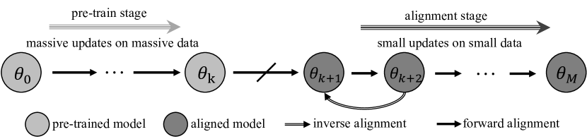
Figure 1: Forward and Inverse Alignment. LLMs undergo numerous iterations during pre-training, forming a stable parameter distribution. Subsequent alignment procedures fine-tune this distribution to reflect human intentions. Our research question is: During further fine-tuning, is it harder to deviate from the stable parameter distribution formed during pre-training than to maintain it?

So far, we mainly steer or align models with finetuning-based methods including supervised fine-tuning (SFT), reinforcement learning from human feedback (RLHF) [9], and more [8, 10, 11, 12, 13, 14]. However, it remains unclear whether such methods truly penetrate the model representations or merely perform superficial alignment. Recent studies [15, 16] have shown that the effect of alignment process is superficial, e.g., models undergoing safety alignment can become unsafe again with minimal fine-tuning. Furthermore, fine-tuning aligned LLMs on non-malicious datasets can weaken the models’ safety mechanisms as well [17, 18]. Why is alignment so fragile?

This counterintuitive phenomenon further prompts exploration into the inverse process of alignment: assuming that the alignment process of LLMs is indeed limited to superficial alignment, is it then possible to perform an inverse operation of alignment, i.e., to achieve the reversal of the alignment process through a series of technical measures? In this work, we investigate the possibility of reversing or revoking the alignment process in LLMs, a concept we refer to as unalignment. In a word, we aim to answer the under-explored question:

Do the parameters of language models exhibit elasticity, thereby resisting alignment?

Our main contribution is Theorem 3.13. We show the elasticity of post-alignment models using tools from compression theory, demonstrating that models tend to retain the distribution learned from the pre-train dataset while forgetting the effects of subsequent fine-tuning. We also prove that after subsequent fine-tuning, the changes in the normalized compression rates of the model for different datasets are proportional to their respective sizes. Furthermore, we experimentally demonstrate that the phenomenon of elasticity in post-alignment models is present across models of various scales, emphasizing that when conducting subsequent safety alignment, it is necessary to consider the impact of model elasticity on alignment effectiveness.

2 Background

2.1 Large Language Models

We consider an LLM parameterized by ${\bm{\theta}}$ and denoted by the output distribution $p_{{\bm{\theta}}}(\cdot|\cdot)$. The generation process of the LLM can be defined by $({\mathcal{X}},{\mathcal{Y}},{\mathcal{V}},{\mathcal{L}},p_{{\bm{\theta}}})$. The input space (prompt space) is $\mathcal{X}\in\sum^{\leq l_{\text{max}}}$ , and the output space (response space) is $\mathcal{Y}\in\sum^{\leq l_{\text{max}}}$ for some constant $l_{\text{max}}$. The model takes a sequence ${\bm{x}}=\left(x_{0},\ldots,x_{n-1}\right)$ as input to generate a corresponding output ${\bm{y}}=\left(y_{0},\ldots,y_{m-1}\right)$, where $x_{i}$ and $y_{j}$ represent the individual tokens from a predetermined vocabulary $\Sigma$.

The autoregressive LLM $p_{{\bm{\theta}}}$ generates tokens sequentially for a given position, relying solely on the previously generated tokens sequence. Consequently, this model can be conceptualized as a markov decision process [19], wherein the conditional probability $p_{\theta}({\bm{y}}|{\bm{x}})$ can be defined through a decomposition as follows,

$$p_{{\bm{\theta}}}\left(y_{0..k-1}\big{|}{\bm{x}}\right)=\prod_{0\leq k\leq m}{p_{{\bm{\theta}}}\left(y_{k}\big{|}{\bm{x}},y_{0..k-1}\right)}.$$

Pre-training.

During pre-training, an LLM acquires foundational language comprehension and reasoning abilities by processing vast quantities of unstructured text. The pre-train loss is defined as follows:

$$\mathcal{L}_{\text{PT}}({\bm{\theta}};\mathcal{D}_{\text{PT}})=-\mathbb{E}_{({\bm{x}},x_{N})\sim\mathcal{D}_{\mathrm{PT}}}\left[\log p_{{\bm{\theta}}}\left(x_{N}\big{|}{\bm{x}}\right)\right].$$

where ${\bm{x}}=(x_{0},\cdots,x_{N-1})$ and $N\in\mathbb{N}$, such that $(x_{0},\cdots,x_{N})$ forms a prefix in some piece of pre-training text.

Supervised Fine-tuning (SFT).

This phase adjusts the pre-trained models to follow specific instructions, utilizing a smaller dataset compared to the pre-training corpus to ensure mode alignment with target tasks. For a given SFT dataset $\mathcal{D}_{\mathrm{SFT}}=\left\{\left({\bm{x}}^{i},{\bm{y}}^{i}\right)\right\}_{i=1}^{N}$ which is sampled from a high-quality distribution, SFT aims to minimize the negative log-likelihood loss:

$$\mathcal{L}_{\text{SFT}}({\bm{\theta}};\mathcal{D}_{\text{SFT}})=-\mathbb{E}_{({\bm{x}},\bf{y)\sim\mathcal{D}_{\mathrm{SFT}}}}\left[\log p_{{\bm{\theta}}}\left({\bm{y}}\big{|}{\bm{x}}\right)\right].$$

Given that $\mathbb{E}_{({\bm{x}},\bf{y)\sim\mathcal{D}_{\text{SFT}}}}\left[\log{p_{\mathcal{D}}\left({\bm{y}}\big{|}{\bm{x}}\right)}\right]$ is fixed when specifying $\mathcal{D}_{\text{SFT}}$, the optimization objective $\mathcal{L}_{\text{SFT}}$ becomes the Kullback-Leible (KL) divergence between the model $p_{{\bm{\theta}}}$ and the SFT distribution.

Note that the loss functions for pre-training and SFT are analogous in their essence. Therefore, we will treat them alike in our later analysis.

2.2 Compression Theory

Lossless Compression.

The goal of lossless compression is to find a compression protocol that encodes a given dataset $\mathcal{D}$ and its distribution $\mathcal{P}_{\mathcal{D}}$ with the smallest possible expected length, and allows for a decoding scheme that can perfectly reconstruct the original dataset $\mathcal{D}$ from the compressed data. According to Shannon’s source coding theorem [20], for a random variable takes value from $\mathcal{D}$ and follows $\mathcal{P}_{\mathcal{D}}$, the expected code length $\mathcal{L}$ of any lossless compression protocol satisfies

$$\mathcal{L}\geq H\left(\mathcal{P}_{\mathcal{D}}\right).$$

where $H\left(\mathcal{P}_{\mathcal{D}}\right)$ stands for the Shannon entropy of $\mathcal{P}_{\mathcal{D}}$. Huffman code [21] is a typical type of optimal code for lossless compression. For a random variable follows $\mathcal{P}_{\mathcal{D}}$, the expected code length $\mathcal{L}$ satisfies

$$H\left(\mathcal{P}_{\mathcal{D}}\right)\leq\mathcal{L}\leq H\left(\mathcal{P}_{\mathcal{D}}\right)+1.$$

Compression and Prediction.

The relationship between data compression and prediction is tightly interconnected. Consider a model $p_{{\bm{\theta}}}$ and ${\bm{x}}=\left(x_{0},\cdots,x_{m-1}\right)$ derived from a dataset $\mathcal{D}$. Under arithmetic coding [22, 23], the optimal expected code length $\mathcal{L}$ is given by:

$$\mathcal{L}=\mathbb{E}_{{\bm{x}}\sim\mathcal{D}}\left[\sum_{0\leq k\leq m}-\log_{2}p_{{\bm{\theta}}}\left(x_{i}\big{|}x_{0,\cdots,k-1}\right)\right].$$

This aligns with the cross-entropy loss used when training $p_{{\bm{\theta}}}$, which suggests a certain consistency between compression and prediction. Hutter [24] provides a more detailed explanation of the equivalence between compressing optimal and predicting optimal. Experimentally, further evidence has been provided to demonstrate the equivalence between large language model prediction and compression [22] and establish that compression performance represents intelligence linearly [23].

3 Elasticity in Large Language Models as Resistance to Alignment

In this section, we formulate the concept of elasticity and prove its existence in LLMs. It gives rise to the possibility of inverse alignment, thereby constituting resistance to alignment. We start by defining these concepts.

Definition 3.1 (Inverse Alignment).

Given an initial language model $p_{{\bm{\theta}}_{0}}$, for any $\epsilon$, after aligning it on dataset $\mathcal{D}_{a}$ to obtain the aligned model $p_{{\bm{\theta}}_{1}}$, we use dataset $\mathcal{D}_{b}$ (where $|\mathcal{D}_{b}|\ll|\mathcal{D}_{a}|$) to perform an operation on $p_{{\bm{\theta}}_{1}}$. This process yields an inverse-aligned model $p_{{\bm{\theta}}_{0}^{\prime}}$, such that $\rho(p_{{\bm{\theta}}_{0}^{\prime}},p_{{\bm{\theta}}_{0}})\leq\epsilon$ for a given metric function $\rho$ (which can be viewed as a measure of behavioral and distributional proximity between two models). We define the transition from $p_{{\bm{\theta}}_{1}}$ back to $p_{{\bm{\theta}}_{0}}$ as inverse alignment.

Definition 3.2 (The Elasticity of LLM Parameters).

Given an LLM $p_{{\bm{\theta}}_{0}}$, and the transformation $p_{{\bm{\theta}}_{0}}\xmapsto{f(\mathcal{D}_{a})}p_{{\bm{\theta}}_{1}}$, elasticity is said to exist in $\left(p_{{\bm{\theta}}_{0}},\mathcal{D}_{a}\right)$ if there is an algorithmically simple inverse operation $g$ and a dataset $\mathcal{D}_{b}$ such that $|\mathcal{D}_{b}|\ll|\mathcal{D}_{a}|$, with the property that

$$p_{{\bm{\theta}}_{1}}\xmapsto{g(\mathcal{D}_{b})}p_{{\bm{\theta}}_{0}^{\prime}}\text{~{}and~{}}\rho(p_{{\bm{\theta}}_{0}^{\prime}},p_{{\bm{\theta}}_{0}})\leq\epsilon.$$

3.1 The Token-level Response Tree for Compression Analysis

We explain that the post-alignment models contain elasticity using information-theoretic concepts specifically related to data compression, given the analytical equivalence and practical consistency between compression and prediction performance (Section 2.2).

We first present our formulation for the compression protocol, using tokenized sequences as the input and output modality. Due to space constraints, we selectively present key definitions, assumptions, and theorems. Please refer to Appendix A for the full collection of assumptions and proofs.

Assumption 3.3 (Binary Tokens).

For the purpose of this analysis, consider the tokenization process employed on the datasets. Without loss of generality (since any vocabulary sizes can be approximately reduced to the binary case with a uniform multiplier to the code length), we assume that the token table contains only binary tokens (specifically 0/1) and is uniform across all datasets.

Definition 3.4 (Token-level Response Tree $\mathcal{T}$).

Consider the dataset $\mathcal{D}=\{{\bm{z}}_{i}\in\{0|1\}^{\infty}\mid i=1,2,\cdots\}$, where each ${\bm{z}}_{i}$ represents a binary response in $\mathcal{D}$. The token-level response tree, denoted as $\mathcal{T}_{\mathcal{D}}$, is structured such that each node contains child nodes labeled 0 or 1. Additionally, each binary node terminates with an end-of-sequence (EOS) token leaf node. The path from the root to a leaf node delineates each response ${\bm{z}}_{i}$. The likelihood of a response that a token represents is indicated by the probability associated with its EOS token node. Meanwhile, the probability of any binary node is defined as the sum of the probabilities of all its child nodes.

Remark 3.5 (Pruning of the TRT).

For a pruned node $\mathcal{S}$ of a TRT, the pruning operation is as follows: remove the pruned node and all its children, then add the probability of the node $S$ to its parent’s EOS node. The pruning operation decreases the depth and the number of nodes in the TRT while the sum of the probability of all EOS nodes remains constant at 1.

Remark 3.6 (${\bm{z}}$’s meaning).

Since model compression for datasets involves both pre-training and SFT processes, ${\bm{z}}$ represents different meanings in these two processes. During pre-training, ${\bm{z}}$ represents a complete sequence of text segments; whereas during SFT, ${\bm{z}}$ represents a complete sequence of questions and corresponding answers in the dataset.

Definition 3.7 (Compression with Finite-parameter Models).

For a finite-parameter model $p_{{\bm{\theta}}}\left(\cdot\right)$ and the dataset $\mathcal{D}$, the compression protocol using $p_{{\bm{\theta}}}$ for $\mathcal{D}$ is defined as follows: For $\mathcal{D}$’s TRT $\mathcal{T}_{\mathcal{D}}$, the compression of $\mathcal{D}$ by $p_{{\bm{\theta}}}$ is defined by the following two steps: 1) Prune the $\mathcal{T}_{\mathcal{D}}$ in the manner of Remark 3.5, retaining only the top $d$ layers of $\mathcal{T}_{\mathcal{D}}$, where $d$ is a quantity determined by $p_{{\bm{\theta}}}$’s parameter count. 2) Compress the pruned response tree using Huffman coding. In this scheme, each response from the root token to a 0/1 token is considered as a letter in the Huffman coding alphabet, with the probability of the EOS token for the corresponding 0/1 token serving as the probability of that letter.

Theorem 3.8 (Ideal Code Length with Finite-parameter Models).

Consider a finite parameter model $p_{{\bm{\theta}}}\left(\cdot\right)$ which is training on dataset $\mathcal{D}$, the ideal code length $\mathcal{L}_{p_{{\bm{\theta}}}}\left({\bm{x}}\right)$ of a random response ${\bm{x}}$ compressed by $p_{{\bm{\theta}}}$ can be expressed as follows,

$$\mathbb{E}\left[\mathcal{L}_{p_{{\bm{\theta}}}}\left({\bm{x}}\right)\right]=\left\lceil\frac{\big{|}{\bm{x}}\big{|}}{d}\right\rceil\left\lceil-\sum_{i=1}^{d}\sum_{j=1}^{2^{i-1}}p_{ij}\log{p_{ij}}\right\rceil,$$ (1)

where $d$ represents the depth of the $\mathcal{T}_{\mathcal{D}}$ after pruning under Definition 3.7 protocol, and $p_{ij}$ represents the probability values of the EOS nodes for the $j$-th node at the $i$-th layer.

Definition 3.9 (Compression Rate of Finite-parameter Model).

Consider a finite parameter model $p_{{\bm{\theta}}}\left(\cdot\right)$ which is training on dataset $\mathcal{D}$ that follows the distribution $p_{\mathcal{D}}$, the reciprocal of the data compression rate $\gamma_{p_{{\bm{\theta}}}}$ of the model $p_{{\bm{\theta}}}$ is defined as follows,

$$\gamma_{p_{{\bm{\theta}}}} =\mathbb{E}_{{\bm{x}}}\left[\frac{\mathbb{E}_{{\bm{x}}}\left[\mathcal{L}_{p_{{\bm{\theta}}}}\left({\bm{x}}\right)\right]}{\big{|}{\bm{x}}\big{|}}\right]$$ (2)

$$=\Theta\left(-\frac{\sum_{i=1}^{d}\sum_{j=1}^{2^{i-1}}p_{ij}\log{p_{ij}}}{d}\right),$$ (3)

where $p_{ij},d$ share the same definition as in Theorem 3.8.

3.2 Formal Derivation of Elasticity

We go on to formally show the existence of elasticity in LLMs. We start by formulating multi-stage training with multiple datasets.

Definition 3.10 (Joint Compression of Multiple Datasets).

Consider using a finite parameter model to compress $N$ pairwise disjoint datasets $\mathcal{D}_{1},\cdots,\mathcal{D}_{N}$. For the TRT of the jointly compressed dataset $\mathcal{D}=\bigcup_{k=1}^{N}\mathcal{D}_{k}$, in the context of joint compression, the node weights relate to the node weights of each compressed dataset $\mathcal{D}_{k}$ as follows.

$$p_{i}^{\mathcal{D}}=\frac{\sum_{k=1}^{N}p_{i}^{\mathcal{D}_{k}}\big{|}\mathcal{D}_{k}\big{|}}{\sum_{k=1}^{N}\big{|}\mathcal{D}_{k}\big{|}},$$ (4)

where $p_{i}^{\mathcal{D}}$ stands for the probability value for the node in $\mathcal{T}_{\mathcal{D}}$ while $p_{i}^{\mathcal{D}_{k}}$ stands for the probability value for the node in $\mathcal{T}_{\mathcal{D}_{k}}$. The finite parameter joint compression process for $\mathcal{D}_{1},\cdots,\mathcal{D}_{N}$ is essentially the process of compressing $\mathcal{D}$ according to Definition 3.7.

Definition 3.11 (Compression Rate for Specific Dataset).

For $N$ pairwise disjoint datasets $\mathcal{D}_{1},\cdots,\mathcal{D}_{N}$ and a finite parameter model $p_{{\bm{\theta}}}$ compressing $\mathcal{D}=\bigcup_{k=1}^{N}\mathcal{D}_{k}$, the reciprocal of the compression rate $\gamma_{p_{{\bm{\theta}}}}^{\mathcal{D}_{i}}$ for a particular dataset $\mathcal{D}_{k}$ is defined as follows.

$$\gamma_{p_{{\bm{\theta}}}}^{\mathcal{D}_{i}} =\mathbb{E}_{{\bm{x}}\sim\mathcal{P}_{i}}\left[\frac{\mathbb{E}_{{\bm{x}}\sim\mathcal{P}_{i}}\left[\mathcal{L}_{p_{{\bm{\theta}}}}^{\mathcal{D}_{i}}({\bm{x}})\right]}{\big{|}{\bm{x}}\big{|}}\right]$$ (5)

$$=\mathbb{E}_{{\bm{x}}\sim\mathcal{P}_{i}}\left[\frac{1}{\big{|}{\bm{x}}\big{|}}\left\lceil\frac{\big{|}{\bm{x}}\big{|}}{d}\right\rceil\left\lceil-\sum_{i=1}^{d}\sum_{j=1}^{2^{i-1}}p_{ij}^{\mathcal{D}_{k}}\log{p_{ij}^{\mathcal{D}}}\right\rceil\right]$$ (6)

$$=\Theta\left(-\frac{\sum_{i=1}^{d}\sum_{j=1}^{2^{i-1}}p_{ij}^{\mathcal{D}_{k}}\log{p_{ij}^{\mathcal{D}}}}{d}\right),$$ (7)

where $p_{ij}^{\mathcal{D}_{k}}$ represents the probability values of the EOS nodes for the $j$-th node at the $i$-th layer in $\mathcal{T}_{k}^{\prime}$.

Our primary focus is on studying the behavioral changes of the model during subsequent fine-tuning after pre-training and one round of SFT. Therefore, it can be assumed that in the analysis of model compression, only three datasets are involved: the pre-training dataset $\mathcal{D}_{1}$, the fine-tuning dataset $\mathcal{D}_{2}$ in the first round of SFT, and the perturbation dataset $\mathcal{D}_{3}$ used in subsequent fine-tuning. Without loss of generality, we can consider these three datasets to be independent and differently distributed.

Due to the different scales of compression rates obtained for different datasets by the model, we consider normalizing the compression rates for different datasets.

Definition 3.12 (Normalized Compression Rate).

For $N$ pairwise disjoint datasets $\mathcal{D}_{1},\cdots,\mathcal{D}_{N}$ and a finite parameter model $p_{{\bm{\theta}}}$ compressing $\mathcal{D}=\bigcup_{k=1}^{N}\mathcal{D}_{k}$, the normalized reciprocal of the compression rate $\gamma_{p_{{\bm{\theta}}}}^{\mathcal{D}_{k}/\mathcal{D}}$ for a particular dataset $\mathcal{D}_{k}$ is defined as:

$$\gamma_{p_{{\bm{\theta}}}}^{\mathcal{D}_{k}/\mathcal{D}}=\frac{\gamma_{p_{{\bm{\theta}}}}^{\mathcal{D}_{k}}-\frac{1}{d}\log{2^{d-1}}}{\gamma_{p_{{\bm{\theta}}}}^{\mathcal{D}}-\frac{1}{d}\log{2^{d-1}}},$$ (8)

where $d$ is the depth of the pruned tree $\mathcal{T}_{k}^{\prime}$ of dataset $\mathcal{D}_{k}$. Here, $\frac{1}{d}\log{2^{d-1}}$ is the reciprocal of the compression rate for a uniform distribution while $\gamma_{p_{{\bm{\theta}}}}^{\mathcal{D}}$ represents the reciprocal of the compression rate for $\mathcal{D}$.

Theorem 3.13 (Elasticity of Language Models).

Consider datasets $\mathcal{D}_{1}$, $\mathcal{D}_{2}$, $\mathcal{D}_{3}$ each with a Pareto mass distribution (Assumption A.8), and the model $p_{{\bm{\theta}}}\left(\cdot\right)$ trained on $\mathcal{D}=\mathcal{D}_{1}\cup\mathcal{D}_{2}\cup\mathcal{D}_{3}$. When dataset $\mathcal{D}_{3}$’s data volume $|\mathcal{D}_{3}|$ changes, the normalized reciprocal of the compression ratio $\gamma_{p_{{\bm{\theta}}}}^{\mathcal{D}_{1}/\mathcal{D}}$, $\gamma_{p_{{\bm{\theta}}}}^{\mathcal{D}_{2}/\mathcal{D}}$ of the model for $\mathcal{D}_{1}$ and $\mathcal{D}_{2}$ satisfies:

$$\frac{d\gamma_{p_{{\bm{\theta}}}}^{\mathcal{D}_{2}/\mathcal{D}}}{d\,l} =\Theta\left(k\frac{d\gamma_{p_{{\bm{\theta}}}}^{\mathcal{D}_{1}/\mathcal{D}}}{d\,l}\right)$$ (9)

$$\frac{d\gamma_{p_{{\bm{\theta}}}}^{\mathcal{D}_{1}/\mathcal{D}}}{d\,l} >0,\frac{d\gamma_{p_{{\bm{\theta}}}}^{\mathcal{D}_{2}/\mathcal{D}}}{d\,l}>0$$ (10)

where $l=\frac{|\mathcal{D}_{3}|}{|\mathcal{D}_{2}|}\ll 1$, $k=\frac{|\mathcal{D}_{1}|}{|\mathcal{D}_{2}|}\gg 1$.

Theorem 3.13 illustrates that as the amount of data in the perturbation dataset $\mathcal{D}_{3}$ increases, the normalized compression rates of the model for both the pre-train dataset $\mathcal{D}_{1}$ and the SFT dataset $\mathcal{D}_{2}$ decrease, but the rate of decrease for the pre-train dataset is smaller than that for the SFT dataset by a factor of $\Theta(k)$, which in practice is many orders of magnitude.

This indicates that when faced with interference, the model tends to maintain the distribution contained in the larger dataset, namely the pre-train dataset, and is inclined to forget the distribution contained in the smaller dataset, namely the SFT dataset, which demonstrates the elasticity of language models.

4 Experiments

In the previous sections, we proved that LLMs achieve stable behavioral distributions during the pre-training stage through massive updates on massive data. The alignment stage with small updates on small data does not erase such a distribution, and subsequent fine-tuning can easily restore this pre-alignment distribution. Building on top of this discovery, in this section, we primarily aim to answer the following questions:

• Is inverse alignment easier than forward alignment?

• Does elasticity consistently exist across models of different types and sizes?

• Is elasticity correlated with model parameter size and pre-training data size?

4.1 Comparison between Inverse Alignment and Forward Alignment

In this section, we extract several sliced models during the fine-tuning process and construct twin datasets to perform inverse operations on models at different stages. We aim to verify the behavioral differences between forward and inverse alignment.

4.1.1 Experiment Setup

Tasks and datasets. During the experiment, we select three tasks for extensive testing, including instruction-following [25], TruthfulQA [26], and PKU-SafeRLHF [4]. These tasks correspond to the widely accepted 3H standards (Helpful, Harmless, and Honest) [27] for LLMs. We divide the dataset into four equal parts to obtain four sliced models during the fine-tuning process. In the Harmless and Honest experiments, we pre-fine-tune the model with the 52K Alpaca [25] instruction-following dataset to equip the base model with conversational capabilities.

Model training and inference. We consider Llama2-7B, Llama2-13B [7] and Llama3-8B [28] as the base model $\theta_{0}$. We adopt the AdamW optimizer with $\beta_{1}=0.99$, $\beta_{2}=0.95$, and weight dacay $=0.01$ in all experiments. All models are trained on 8$\times$A800 GPUs. During inference, we use the parameters of top-k:30, top-p:0.9, and temperature:0.1.

4.1.2 Experiment Design

As shown in Figure 2, we consider two sliced models during the fine-tuning process. Measuring the transition from model $\theta_{k+1}$ to model $\theta_{k+2}$ is straightforward, considering factors such as data volume, update steps, and parameter distribution. However, measuring the transition from model $\theta_{k+2}$ to model $\theta_{k+1}$, i.e., inverse alignment, is difficult. To address this challenge, we design the following experiment: we fine-tune models based on $\theta_{k+1}$ and $\theta_{k+2}$ to derive $\theta_{k+1}^{\prime}$ and $\theta_{k+2}^{\prime}$, which we designate as path $A$ and path $B$, respectively. Specifically, we use a shared query set $Q$ for paths $A$ and $B$.

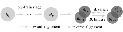
Figure 2: Parameter evaluation over slice models.

Path A. Responses generated by $\theta_{k+1}$ based on $Q$ are used to form $Q-A^{\theta_{k+1}}$ pairs for path $A$’s inverse alignment.

Path B. Similarly, responses generated by $\theta_{k+2}$ based on $Q$ are used to form $Q-A^{\theta_{k+2}}$ pairs for path $B$’s forward alignment.

Given that paths $A$ and $B$ have identical training hyper-parameters and query set, we can assess the differences between $\theta_{k+1}^{\prime}$ and $\theta_{k+1}$ (represented by $\delta_{k+1}$), and between $\theta_{k+2}^{\prime}$ and $\theta_{k+2}$ (represented by $\delta_{k+2}$), utilizing the same training steps. If $\delta_{k+2}$ is consistently greater than $\delta_{k+1}$, it suggests that $\theta_{k+1}^{\prime}$ aligns more closely with $\theta_{k+1}$. Consequently, inverse alignment proves more effective with the same training step than forward alignment. We use cross-entropy as the distance metric when calculating $\delta_{k+1}$ and $\delta_{k+2}$.

4.1.3 Experiment Results

Table 1: Comparsion between inverse alignment and forward alignment.

Datasets	Base Models	$H(p_{\theta_{1}},p_{\theta_{21}^{{\dagger}}})$ vs. $H(p_{\theta_{2}},p_{\theta_{12}^{{\dagger}}})$	$H(p_{\theta_{2}},p_{\theta_{32}^{{\dagger}}})$ vs. $H(p_{\theta_{3}},p_{\theta_{23}^{{\dagger}}})$	$H(p_{\theta_{1}},p_{\theta_{31}^{{\dagger}}})$ vs. $H(p_{\theta_{3}},p_{\theta_{13}^{{\dagger}}})$
Instruction-Following	Llama2-7B	0.1589 vs. 0.2018	0.1953 vs. 0.2143	0.1666 vs. 0.2346
	Llama2-13B	0.1772 vs. 0.1958	0.2149 vs. 0.2408	0.1835 vs. 0.2345
	Llama3-8B	0.2540 vs. 0.2573	0.2268 vs. 0.3229	0.2341 vs. 0.2589
Truthful	Llama2-7B	0.1909 vs. 0.2069	0.1719 vs. 0.1721	0.2011 vs. 0.2542
	Llama2-13B	0.1704 vs. 0.1830	0.1544 vs. 0.1640	0.1825 vs. 0.2429
	Llama3-8B	0.2118 vs. 0.2256	0.2100 vs. 0.2173	0.2393 vs. 0.2898
Safe	Llama2-7B	0.2730 vs. 0.2809	0.2654 vs. 0.2691	0.2845 vs. 0.2883
	Llama2-13B	0.2419 vs. 0.2439	0.2320 vs. 0.2327	0.2464 vs. 0.2606
	Llama3-8B	0.2097 vs. 0.2156	0.2008 vs. 0.2427	0.2277 vs. 0.2709

As shown in Table 1, the experimental results show that $\delta_{k+1}$ is smaller than $\delta_{k+2}$ across all three dimensions of the three types of models with all three types datasets. In addition to the comparisons mentioned in the experimental design, to eliminate the influence of model differences on the comparison between inverse alignment and forward alignment, we also compare $\theta_{1}$ with $\theta_{3}$, whose difference corresponds to $\delta_{k+1}$ and $\delta_{k+3}$ in the experimental design. The results are also as expected. All experimental results demonstrate that inverse alignment is easier than forward alignment across diverse models and datasets.

4.2 Analysis of Elasticity

In this experiment, we aim to verify the existence of elasticity across models of various types and sizes. Furthermore, we demonstrate that elasticity tends to increase with either 1) increased model parameter scale, or 2) increased pre-training data volume.

4.2.1 Experiment Setup

Tasks and Datasets. We select two tasks: positive generation and single-turn safe conversation. For the former, we use the data classified as positive or negative in the IMDb dataset [29]. Referring to [8], we use the first 2-8 tokens of each complete text as a prompt for LLMs to generate the subsequent content. For the latter, we use the data classified as safe and unsafe in PKU-SafeRLHF [4]. We organize the positive sample sizes into {1000, 2000, 5000, 10000}, while the negative sample sizes, being fewer in number, were divided into {100, 200, 500, 1000, 2000}.

Model Training and Inference. We first verify elasticity in popular pre-trained LLMs, Gemma-2B [30] and Llama2-7B [7]. Subsequently, we examine the relationship between elasticity and model size using Qwen models [31] across sizes of 0.5B, 4B, and 7B. Finally, to analyze the connection between elasticity and the amount of pre-training data, we conduct further experiments on the 2.0T, 2.5T, and 3.0T slices of TinyLlama [32].

Evaluation and Metrics. We collect the model’s responses on the reserved test prompts. Then we use score models provided by existing research to complete the performance evaluation. For positive style generation, we refer to [8] and use the Sentiment Roberta model [33] to classify the responses, taking the proportion of all responses classified as positive as the model score. For single-turn safe dialogue, we use the cost model provided by [12] to score the safety of each response, using the average score of all responses as the model score.

4.2.2 Experiment Results

Existence of Elasticity. We evaluate the elasticity phenomenon on Llama2-7B [7] and Gemma-2B [30]. The experimental results in Figure 3 show that, for models fine-tuned with a large amount of positive sample data, only a small amount of negative sample fine-tuning is needed to quickly revert to the pre-training distribution, i.e., to make the curve drop below the gray dashed line. Subsequently, the rate of performance decline slows down and tends to stabilize.

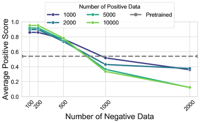
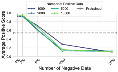
(a) IMDb Experimental Results.

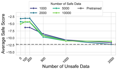
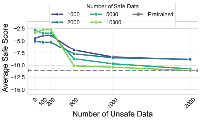
(b) PKU SafeRLHF Experimental Results.

Figure 3: Experimental Results for Validating the Existence of Elasticity. The left and right sides of each subfigure correspond to the performance of Gemma-2B [30] and Llama2-7B [7], respectively, while the caption identifies the dataset. The model performance rapidly declines before reverting to the pre-training distribution, after which the decline becomes significantly slower. This phenomenon is defined as the elasticity of LLMs.

Elasticity Increases with Model Size. To examine how elasticity changes with model parameter size, we conducted experiments on Qwen models [31] with 0.5B, 4B, and 7B parameters. In Figure 4, as the model parameter size increases, the initial performance decline due to negative data fine-tuning is faster, while the subsequent decline is slower. This indicates that as the parameter size increases, there is an increased elasticity in response to both positive and negative data.

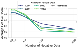
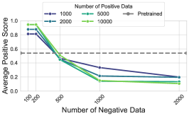
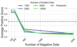
(a) IMDb Experimental Results.

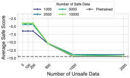
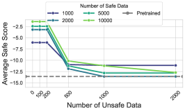
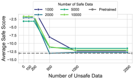
(b) PKU SafeRLHF Experimental Results.

Figure 4: Experimental Results for Validating the Positive Correlation Between Elasticity and Model Parameter Size. Each subfigure from left to right shows the changes in LLMs with parameter sizes of 0.5B, 4B, and 7B, respectively, while the caption identifies the dataset.

Elasticity Increases with Pre-training Data Amount. To verify that elasticity increases with the growth of pre-training data, we conduct the same experiments on multiple pre-training slices released by TinyLlama [32]. As shown in Figure 5, when the pre-training data volume increases, the initial performance decline due to negative data fine-tuning is faster, while the subsequent decline is slower. It demonstrates that larger pre-training data volumes reinforce the elasticity of LLMs.

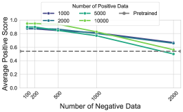
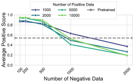
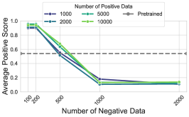
(a) IMDb Experimental Results.

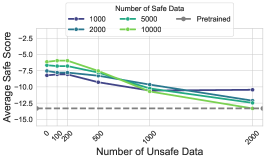
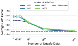
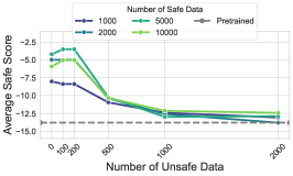
(b) PKU SafeRLHF Experimental Results.

Figure 5: Experimental Results for Validating the Positive Correlation Between Elasticity and Pre-training Data Size. Each subfigure from left to right shows the changes in pre-training data sizes of 2.0T, 2.5T, and 3.0T, while the caption identifies the dataset.

5 Related Work

The Fragility of LLMs Alignment.   Pre-trained LLMs often generate offensive content [6]. Recent initiatives [9, 3] have aimed to align these models to minimize harmful outputs [3, 34]. However, studies show that even well-aligned models can be compromised easily, and fine-tuning them on non-malicious datasets might unintentionally impair their safety mechanisms [15, 17, 35]. Why is alignment so fragile? [36] pinpoint areas essential for safety guardrails distinct from utility-relevant regions, achieving this separation at both neuron and rank levels through weight attribution.

Machine Unlearning.  The necessity for Machine Unlearning (MU) stems from the requirement for adaptive learning systems to erase user privacy data and any derived lineage data [37]. This technique is employed in data deletion [38], enhances the fairness of models [39, 40], and prevents generative models from creating harmful content [4]. Current MU methods can be categorized into two families: exact MU and approximate MU [41, 42]. Exact MU seeks to eliminate the influence of specific data points entirely through comprehensive retraining, offering provable error guarantees for data removal. Conversely, Approximate MU aims to reduce data point influence through efficient parameter updates, trading off complete erasure for lower computational demands [43].

6 Conclusion and Outlook

In this work, prompted by the fragility of alignment, we show the existence of elasticity in language models though both theoretical and experimental lens, thereby demonstrating their tendency to resist alignment. Specifically, large pre-training datasets and large parameter counts enhance the model’s anti-interference capabilities, making subsequent alignment procedures easy to undo via further finetuning. We experiment on a variety of models and datasets, and validate elasticity across different sliced models during pre-training and alignment. Extensive results confirm that language models exhibit elasticity, indicating that language models resist alignment.

6.1 Limitations and Future Work

Theory-wise, the primary limitation of our work is our specification of the mass distribution (Assumption A.8), and empirical studies on the exact form of this distribution shall be valuable. Experiment-wise, we have not systematically validated elasticity throughout the entire lifecycle of pre-training and alignment phases, due to cost constraints. In future works, we plan to focus more on whether this phenomenon is universally applicable, such as in multimodal models. Additionally, we aim to theoretically uncover the relationship between model elasticity and scaling laws, specifically determining the amount of training data required for elasticity to manifest and quantitatively analyzing whether elasticity intensifies as model parameters increase.

6.2 Broader Impacts

Rethinking Fine-tuning.

The influence of noisy pre-training corpora may cause models to exhibit unexpected behaviors. Alignment methods seek to modify LLMs’ distributions efficiently to enhance helpfulness, harmlessness, and honesty. From the inverse alignment perspective, we need more robust methods to ensure that modifications to model parameters go beyond superficial changes. However, certain inducement measures might compromise the alignment strategy, potentially causing severe harm. Additionally, we should prioritize data cleansing during pre-training, rigorously managing noisy and biased data to enhance the malleability of the model’s final distribution [44, 17].

Rethinking Open-sourcing.

Open-sourcing is a double-edged sword [45]. On one hand, it can pose significant risks, such as model misuse, which could endanger public safety through fine-tuning for malicious purposes [46] or system jailbreaking [47]. On the other hand, restricting access may foster monopolistic practices, while open-sourcing cutting-edge models promote a robust open-source community and enhance the usability of these models. Furthermore, it facilitates the decentralization of AI technology [48]. From the perspective of model robustness, well-aligned models can be rendered unsafe with a very small amount of unsafe data. Also, fine-tuning aligned LLMs on non-malicious datasets can weaken the models’ safety mechanisms [49]. Ensuring that open-source models are not misused is a critical challenge, and discoveries in this work prompt the community to build robust alignment algorithms, thereby overcoming the model’s tendency to resist alignment.

Appendix A Assumptions and Proofs

Assumption A.1 (Scale of $\mathcal{T}$ is Monotone with Model Size).

Consider a parameterized model $p_{{\bm{\theta}}}\left(\cdot\right)$, the dataset $\mathcal{D}$ and $\mathcal{D}$’s TRT $\mathcal{T}_{\mathcal{D}}$. Due to the finite size of model parameters ${\bm{\theta}}$, the model $p_{{\bm{\theta}}}$ can only represent a limited portion of $\mathcal{D}$, which corresponds to a finite pruning of the tree $\mathcal{T}_{\mathcal{D}}$. Let’s assume that the depth of the pruned tree $\mathcal{T}_{\mathcal{D}}^{\prime}$ is monotonically increasing with the size of ${\bm{\theta}}$.

Theorem A.2 (Ideal Code Length with Finite-parameter Model).

Consider a finite parameter model $p_{{\bm{\theta}}}\left(\cdot\right)$ which is training on dataset $\mathcal{D}$, the ideal code length $\mathcal{L}_{p_{{\bm{\theta}}}}\left({\bm{x}}\right)$ of a random response ${\bm{x}}$ compressed by $p_{{\bm{\theta}}}$ can be expressed as follows,

$$\mathbb{E}\left[\mathcal{L}_{p_{{\bm{\theta}}}}\left({\bm{x}}\right)\right]=\left\lceil\frac{\big{|}{\bm{x}}\big{|}}{d}\right\rceil\left\lceil-\sum_{i=1}^{d}\sum_{j=1}^{2^{i-1}}p_{ij}\log{p_{ij}}\right\rceil$$ (11)

where $d$ represents the depth of the $\mathcal{T}_{\mathcal{D}}$ after pruning under Definition 3.7 protocol, $p_{ij}$ represents the probability values of the EOS nodes for the $j$-th node at the $i$-th layer.

Proof.

When $\big{|}{\bm{x}}\big{|}\leq d$, the compression protocol defined in Definition 3.7 can perfectly compress ${\bm{x}}$. Hence, the expectation of the ideal code length $\mathcal{L}_{p_{{\bm{\theta}}}}\left({\bm{x}}\right)$ satisfies:

$$\mathbb{E}\left[\mathcal{L}_{p_{{\bm{\theta}}}}\left({\bm{x}}\right)\right]=\left\lceil-\sum_{i=1}^{d}\sum_{j=1}^{2^{i-1}}p_{ij}\log{p_{ij}}\right\rceil$$ (12)

where $d$ represents the depth of the pruned tree $\mathcal{T}_{\mathcal{D}}^{\prime}$ and $p_{ij}$ represents the probability values of the EOS nodes for the $j$-th node at the $i$-th layer.

Now consider $sd\leq\big{|}{\bm{x}}\big{|}\leq(s+1)d$. Let us suppose that ${\bm{x}}=({\bm{x}}_{1}\cdots{\bm{x}}_{s}{\bm{x}}_{s+1})$, where $|{\bm{x}}_{k}|=d$, for $k\in\{1,\ldots,s\}$ and $|{\bm{x}}_{s+1}|\leq d$. In this case, ${\bm{x}}$ cannot be perfectly compressed by the model. Hence, the compression of $x$ needs to be performed in segments, and the length of each segment is not greater than $d$.

$$\mathbb{E}_{{\bm{x}}}\left[\mathcal{L}_{p_{{\bm{\theta}}}}\left({\bm{x}}\right)\right] =\mathbb{E}_{{\bm{x}}_{1}}\left[\mathcal{L}_{p_{{\bm{\theta}}}}\left({\bm{x}}_{1}\right)\right]+\mathbb{E}_{{\bm{x}}_{1}}\mathbb{E}_{({\bm{x}}_{2}\ldots{\bm{x}}_{s+1})}\left[\mathcal{L}_{p_{{\bm{\theta}}}}\left(\left({\bm{x}}_{2}\ldots{\bm{x}}_{s+1}\right)\right)\big{|}{\bm{x}}_{1}\right]$$ (13)

$$=\mathbb{E}_{{\bm{x}}_{1}}\left[\mathcal{L}_{p_{{\bm{\theta}}}}\left({\bm{x}}_{1}\right)\right]+\sum_{{\bm{x}}_{1}}p({\bm{x}}_{1})\sum_{({\bm{x}}_{2}\ldots{\bm{x}}_{s+1})}p({\bm{x}}_{2}\ldots{\bm{x}}_{s+1}\big{|}{\bm{x}}_{1})\cdot\mathcal{L}_{p_{{\bm{\theta}}}}\left(({\bm{x}}_{2}\ldots{\bm{x}}_{s+1})\right)$$ (14)

$$=\mathbb{E}_{{\bm{x}}_{1}}\left[\mathcal{L}_{p_{{\bm{\theta}}}}\left({\bm{x}}_{1}\right)\right]+\sum_{({\bm{x}}_{1}\ldots{\bm{x}}_{s+1})}\frac{p({\bm{x}}_{1}\ldots{\bm{x}}_{s+1})\cdot p({\bm{x}}_{1})}{p({\bm{x}}_{1})}\cdot\mathcal{L}_{p_{{\bm{\theta}}}}\left(({\bm{x}}_{2}\ldots{\bm{x}}_{s+1})\right)$$ (15)

$$=\mathbb{E}_{{\bm{x}}_{1}}\left[\mathcal{L}_{p_{{\bm{\theta}}}}\left({\bm{x}}_{1}\right)\right]+\sum_{({\bm{x}}_{2}\ldots{\bm{x}}_{s+1})}p({\bm{x}}_{2}\ldots{\bm{x}}_{s+1})\cdot\mathcal{L}_{p_{{\bm{\theta}}}}\left(({\bm{x}}_{2}\ldots{\bm{x}}_{s+1})\right)$$ (16)

$$=\mathbb{E}_{{\bm{x}}_{1}}\left[\mathcal{L}_{p_{{\bm{\theta}}}}\left({\bm{x}}_{1}\right)\right]+\mathbb{E}_{({\bm{x}}_{2}\ldots{\bm{x}}_{s+1})}\left[\mathcal{L}_{p_{{\bm{\theta}}}}\left(\left({\bm{x}}_{2}\ldots{\bm{x}}_{s+1}\right)\right)\right]$$ (17)

$$=\sum_{k=1}^{s+1}\mathbb{E}_{{\bm{x}}_{k}}\left[\mathcal{L}_{p_{{\bm{\theta}}}}\left({\bm{x}}_{k}\right)\right]$$ (18)

$$=\left\lceil\frac{\big{|}{\bm{x}}\big{|}}{d}\right\rceil\left\lceil-\sum_{i=1}^{d}\sum_{j=1}^{2^{i-1}}p_{ij}\log{p_{ij}}\right\rceil$$ (19)

thus the proof is completed. ∎

Assumption A.3 (Leaf Node Probability Concentration).

Consider the TRT of dataset $D$. Due to the high proportion of long texts in the dataset , we assume that the probability density of the pruned tree $\mathcal{T}_{\mathcal{D}}^{\prime}$ with depth $d$ is concentrated at the leaf nodes. Let the EOS token probabilities at the leaf nodes of $\mathcal{T}_{\mathcal{D}}^{\prime}$ be denoted as $p_{1},\cdots,p_{2^{d-1}}$, the assumption implies that,

$$\sum_{i=1}^{2^{d-1}}p_{i}=1$$ (20)

Definition A.4 (Mass Distribution in TRT).

Consider the sample space $\Omega$ consisting of all responses in dataset $\mathcal{D}$. The probability distribution $\mathcal{P}_{\mathcal{D}}$ of all subtrees at the $d$-th level nodes of $\mathcal{T}_{\mathcal{D}}$ is a mapping from $\Omega$ to $[0,1]$. Let $X_{\mathcal{D}}$ be the random variable representing the probability value taken at each leaf. The mass distribution $P_{mass}$ represents the probability that $X_{\mathcal{D}}$ takes the corresponding probability value. According to the definition of $P_{mass}$, $\mathbb{E}[X_{\mathcal{D}}]=1$

Remark A.5 (Mixture of Mass Distribution).

For independently and differently distributed datasets $\mathcal{D}_{1},\ldots,\mathcal{D}_{N}$, $\mathcal{D}=\bigcup_{i=1}^{N}\mathcal{D}_{i}$ is a mixture of these datasets. According to Definition 3.10, for the pruned trees $\mathcal{T}_{1},\ldots,\mathcal{T}_{N}$ of these datasets with depth $d$, the random variables of their leaf nodes satisfy the following relationship:

$$X_{\mathcal{D}}=\frac{\sum_{k=1}^{N}\big{|}\mathcal{D}_{k}\big{|}X_{\mathcal{D}_{k}}}{\sum_{k=1}^{N}\big{|}\mathcal{D}_{k}\big{|}}$$ (21)

where $X_{\mathcal{D}_{k}}$ follows the mass distribution $\mathcal{P}_{mass}^{k}$. For $X_{\mathcal{D}_{k_{1}}}$ and $X_{\mathcal{D}_{k_{2}}}$ from different datasets, $X_{\mathcal{D}_{k_{1}}}$ and $X_{\mathcal{D}_{k_{2}}}$ are independent of each other.

Lemma A.6 (Entropy of Mass Distribution).

Consider the pruned trees $\mathcal{T}^{\prime}$ and $\mathcal{T}_{k}^{\prime}$ of dataset $\mathcal{D}$ and $\mathcal{D}=\bigcup_{i=1}^{N}\mathcal{D}_{i}$, both with depth $d$. Denote that the response distribution of the leaf nodes of $\mathcal{T}^{\prime}$ is $\mathcal{P}^{\mathcal{D}}$, and the mass distribution is $\mathcal{P}_{mass}$. Similarly, the response distribution of the leaf nodes of $\mathcal{T}_{k}^{\prime}$ is $\mathcal{P}^{\mathcal{D}}_{k}$, and the mass distribution is $\mathcal{P}_{mass}^{k}$. When $d$ is sufficiently large, the Shannon entropy of the response distribution can be rewritten as follows.

$$\mathbb{E}_{{\bm{x}}\sim\mathcal{P}_{k}}\left[-p^{\mathcal{D}_{k}}\log{p^{\mathcal{D}}}\right]=\mathbb{E}_{X_{\mathcal{D}_{k}}\sim\mathcal{P}_{mass}^{k},X_{\mathcal{D}}\sim\mathcal{P}_{mass}}\left[-X_{\mathcal{D}_{k}}\log{X_{\mathcal{D}}}\right]+\log{2^{d-1}}$$ (22)

where $p^{\mathcal{D}}$, $p^{\mathcal{D}_{k}}$ stand for the probability of the leaf nodes of $\mathcal{T}^{\prime}$,$\mathcal{T}_{k}^{\prime}$ while $X_{\mathcal{D}_{k}}$, $X_{\mathcal{D}}$ stand for the random variables of the probability of the leaf nodes of $\mathcal{T}^{\prime}$,$\mathcal{T}_{k}^{\prime}$.

Proof.

Let $M=2^{d-1}$ be the number of leaf nodes of $\mathcal{T}^{\prime}$ with depth $d$. According to the definitions of the response distribution $\mathcal{P}$ and mass distribution $\mathcal{P}_{mass}$, we have $Mp^{\mathcal{D}_{j}}=X_{\mathcal{D}_{j}},\forall j\in\{1,\dots,N\}$. Therefore,

$$\mathbb{E}_{{\bm{x}}\sim\mathcal{P}_{k}}\left[-p^{\mathcal{D}_{k}}\log{p^{\mathcal{D}}}\right] =\sum_{i=1}^{M}-p_{i}^{\mathcal{D}_{k}}\log{p_{i}^{\mathcal{D}}}$$ (23)

$$=\sum_{i=1}^{M}-\frac{X_{i,\mathcal{D}_{k}}}{M}\log{\frac{X_{i,\mathcal{D}}}{M}}$$ (24)

$$=\sum_{i=1}^{M}-\frac{1}{M}X_{i,\mathcal{D}_{k}}\log{X_{i,\mathcal{D}_{k}}}+\log{M}$$ (25)

$$=\mathbb{E}_{X_{\mathcal{D}_{k}}\sim\mathcal{P}_{mass}^{k},X_{\mathcal{D}}\sim\mathcal{P}_{mass}}\left[-X_{\mathcal{D}_{k}}\log{X_{\mathcal{D}}}\right]+\log{2^{d-1}}$$ (26)

∎

Remark A.7.

In Lemma A.6, $X_{\mathcal{D}_{k}}$ are assumed to be independent. However due to $\sum_{i=1}^{M}p_{i}^{\mathcal{D}_{k}}=1$, the $X_{\mathcal{D}_{k}}$ are not actually independent. Considering that $d$ is sufficiently large in our subsequent analysis, we can regard the independence of $X_{\mathcal{D}_{k}}$ as a good approximation.

Assumption A.8 (Introduction of Pareto Distribution).

We assume that the mass distribution of the segment follows a heavy-tailed Pareto distribution, with supporting evidence from [50, 51]. In this paper, we assume that the mass distribution of the pruned trees $\mathcal{T}^{\prime}$ of the same depth $d$ from different datasets follows a Pareto distribution with the same parameters.

$$p_{X}(x)=\begin{cases}\frac{\alpha C^{\alpha}}{x^{\alpha+1}}&x\geq C,\\ 0&x<C.\end{cases}$$ (27)

where $\alpha,C$ are parameters of the Pareto distribution. Here we assume that $\alpha$ is sufficiently large due to the lighter heavy-tailed nature of the mass distribution.

Theorem A.9 (Elasticity of Language Models).

Consider datasets $\mathcal{D}_{1}$, $\mathcal{D}_{2}$, $\mathcal{D}_{3}$ each with a Pareto mass distribution (Assumption A.8), and the model $p_{{\bm{\theta}}}\left(\cdot\right)$ trained on $\mathcal{D}=\mathcal{D}_{1}\cup\mathcal{D}_{2}\cup\mathcal{D}_{3}$. When dataset $\mathcal{D}_{3}$’s data volume $|\mathcal{D}_{3}|$ changes, the normalized reciprocal of the compression ratio $\gamma_{p_{{\bm{\theta}}}}^{\mathcal{D}_{1}/\mathcal{D}}$, $\gamma_{p_{{\bm{\theta}}}}^{\mathcal{D}_{2}/\mathcal{D}}$ of the model for $\mathcal{D}_{1}$ and $\mathcal{D}_{2}$ satisfies:

$$\frac{d\gamma_{p_{{\bm{\theta}}}}^{\mathcal{D}_{2}/\mathcal{D}}}{d\,l} =\Theta\left(k\frac{d\gamma_{p_{{\bm{\theta}}}}^{\mathcal{D}_{1}/\mathcal{D}}}{d\,l}\right)$$ (28)

$$\frac{d\gamma_{p_{{\bm{\theta}}}}^{\mathcal{D}_{1}/\mathcal{D}}}{d\,l} >0$$ (29)

$$\frac{d\gamma_{p_{{\bm{\theta}}}}^{\mathcal{D}_{2}/\mathcal{D}}}{d\,l} >0$$ (30)

where $l=\frac{|\mathcal{D}_{3}|}{|\mathcal{D}_{2}|}\ll 1$, $k=\frac{|\mathcal{D}_{1}|}{|\mathcal{D}_{2}|}\gg 1$.

Proof.

For the sake of convenience in calculations, we first use Lemma A.6 to replace the Shannon entropy of response distribution.

$$\frac{d\gamma_{p_{{\bm{\theta}}}}^{\mathcal{D}_{j}/\mathcal{D}}}{d\,l} =\frac{d\left(\frac{\mathbb{E}_{{\bm{x}}\sim\mathcal{P}_{j}}\left[-p^{\mathcal{D}_{j}}\log{p^{\mathcal{D}}}\right]-\log{2^{d-1}}}{\mathbb{E}_{{\bm{x}}\sim\mathcal{P}}\left[-p^{\mathcal{D}}\log{p^{\mathcal{D}}}\right]-\log{2^{d-1}}}\right)}{d\,l}$$ (31)

$$=\frac{d\left(\frac{\mathbb{E}_{X_{\mathcal{D}_{j}}\sim\mathcal{P}_{mass}^{j},X_{\mathcal{D}}\sim\mathcal{P}_{mass}}\left[-X_{\mathcal{D}_{j}}\log{X_{\mathcal{D}}}\right]}{\mathbb{E}_{X_{\mathcal{D}}\sim\mathcal{P}_{mass},X_{\mathcal{D}}\sim\mathcal{P}_{mass}}\left[-X_{\mathcal{D}}\log{X_{\mathcal{D}}}\right]}\right)}{d\,l}.$$ (32)

According to Assumption A.8, $X_{D_{j}}$ follows a Pareto distribution with the same parameters $\alpha$ and $c$. Hence,

$$\mathbb{E}_{X_{\mathcal{D}_{j}}\sim\mathcal{P}_{mass}^{j},X_{\mathcal{D}}\sim\mathcal{P}_{mass}}\left[-X_{\mathcal{D}_{j}}\log{X_{\mathcal{D}}}\right]$$ (33)

$$=-\int_{c}^{+\infty}\int_{c}^{+\infty}\int_{c}^{+\infty}\frac{\alpha^{3}c^{3\alpha}x_{j}}{\prod_{i=1}^{3}x_{i}^{\alpha+1}}\log{\frac{\sum_{i=1}^{3}\big{|}\mathcal{D}_{i}\big{|}x_{i}}{\sum_{i=1}^{3}\big{|}\mathcal{D}_{i}\big{|}}}dx_{1}dx_{2}dx_{3}$$ (34)

$$=-\int_{c}^{+\infty}\int_{c}^{+\infty}\int_{c}^{+\infty}\frac{\alpha^{3}c^{3\alpha}x_{j}}{\prod_{i=1}^{3}x_{i}^{\alpha+1}}\log{\frac{kx_{1}+x_{2}+lx_{3}}{k+l+1}}dx_{1}dx_{2}dx_{3}$$ (35)

$$\mathbb{E}_{X_{\mathcal{D}}\sim\mathcal{P}_{mass}^{,}X_{\mathcal{D}}\sim\mathcal{P}_{mass}}\left[-X_{\mathcal{D}}\log{X_{\mathcal{D}}}\right]$$ (36)

$$=-\int_{c}^{+\infty}\int_{c}^{+\infty}\int_{c}^{+\infty}\frac{\alpha^{3}c^{3\alpha}}{\prod_{i=1}^{3}x_{i}^{\alpha+1}}\cdot\frac{kx_{1}+x_{2}+lx_{3}}{k+l+1}\log{\frac{kx_{1}+x_{2}+lx_{3}}{k+l+1}}dx_{1}dx_{2}dx_{3},$$ (37)

where $j=1,2,3$. Therefore, $\frac{d\gamma_{p_{{\bm{\theta}}}}^{\mathcal{D}_{1}/\mathcal{D}}}{d\,l}$ and $\frac{d\gamma_{p_{{\bm{\theta}}}}^{\mathcal{D}_{2}/\mathcal{D}}}{d\,l}$ can be written as:

$$\frac{d\gamma_{p_{{\bm{\theta}}}}^{\mathcal{D}_{1}/\mathcal{D}}}{d\,l}=\frac{\frac{dS_{1}}{d\;l}H-\frac{dH}{d\;l}S_{1}}{H^{2}}$$ (38)

$$\frac{d\gamma_{p_{{\bm{\theta}}}}^{\mathcal{D}_{2}/\mathcal{D}}}{d\,l}=\frac{\frac{dS_{2}}{d\;l}H-\frac{dH}{d\;l}S_{2}}{H^{2}},$$ (39)

where

$$H= \int_{c}^{+\infty}\int_{c}^{+\infty}\int_{c}^{+\infty}\frac{kx_{1}+x_{2}+lx_{3}}{x_{1}^{\alpha+1}x_{2}^{\alpha+1}x_{3}^{\alpha+1}(k+l+1)}\log{\frac{kx_{1}+x_{2}+lx_{3}}{k+l+1}}dx_{1}dx_{2}dx_{3}$$ (40)

$$S_{1}= \int_{c}^{+\infty}\int_{c}^{+\infty}\int_{c}^{+\infty}\frac{1}{x_{1}^{\alpha}x_{2}^{\alpha+1}x_{3}^{\alpha+1}}\log{\frac{kx_{1}+x_{2}+lx_{3}}{k+l+1}}dx_{1}dx_{2}dx_{3}$$ (41)

$$S_{2}= \int_{c}^{+\infty}\int_{c}^{+\infty}\int_{c}^{+\infty}\frac{1}{x_{1}^{\alpha+1}x_{2}^{\alpha}x_{3}^{\alpha+1}}\log{\frac{kx_{1}+x_{2}+lx_{3}}{k+l+1}}dx_{1}dx_{2}dx_{3}.$$ (42)

Proving that $\frac{d\gamma_{p_{{\bm{\theta}}}}^{\mathcal{D}_{2}/\mathcal{D}}}{d\,l}=\Theta\left(k\frac{d\gamma_{p_{{\bm{\theta}}}}^{\mathcal{D}_{1}/\mathcal{D}}}{d\,l}\right)$ is equivalent to proving:

$$\lim_{k\to+\infty,\,l\to 0}\frac{k\cdot\frac{d\gamma_{p_{{\bm{\theta}}}}^{\mathcal{D}_{1}/\mathcal{D}}}{d\,l}}{\frac{d\gamma_{p_{{\bm{\theta}}}}^{\mathcal{D}_{2}/\mathcal{D}}}{d\,l}}=C$$ (43)

where $C$ is a constant. By substituting (38) and (39) into (43), we have

$$\lim_{k\to+\infty,\,l\to 0}\frac{k\cdot\frac{d\gamma_{p_{{\bm{\theta}}}}^{\mathcal{D}_{1}/\mathcal{D}}}{d\,l}}{\frac{d\gamma_{p_{{\bm{\theta}}}}^{\mathcal{D}_{2}/\mathcal{D}}}{d\,l}}=\frac{\lim_{k\to+\infty,\,l\to 0}k\left(\frac{dS_{1}}{d\;l}H-\frac{dH}{d\;l}S_{1}\right)}{\lim_{k\to+\infty,\,l\to 0}\frac{dS_{2}}{d\;l}H-\frac{dH}{d\;l}S_{2}}$$ (44)

Now calculate the values of $S_{1}$, $S_{2}$, $H$ and $\frac{dS_{1}}{d\;l}$, $\frac{dS_{2}}{d\;l}$, $\frac{dH}{d\;l}$ respectively in the case of $k\to+\infty,\,l\to 0$.

$$\lim_{k\to+\infty,\,l\to 0}S_{1}$$

$$= \lim_{k\to+\infty,\,l\to 0}\int_{c}^{+\infty}\int_{c}^{+\infty}\int_{c}^{+\infty}\frac{1}{x_{1}^{\alpha}x_{2}^{\alpha+1}x_{3}^{\alpha+1}}\log{\frac{kx_{1}+x_{2}+lx_{3}}{k+l+1}}dx_{1}dx_{2}dx_{3}$$ (45)

$$= \int_{c}^{+\infty}\int_{c}^{+\infty}\lim_{k\to+\infty,\,l\to 0}\int_{c}^{\delta(kx_{1}+x_{2})}\frac{1}{x_{1}^{\alpha}x_{2}^{\alpha+1}x_{3}^{\alpha+1}}\log{\frac{kx_{1}+x_{2}+lx_{3}}{k+l+1}}dx_{3}dx_{1}dx_{2}$$ (46)

$$= \int_{c}^{+\infty}\int_{c}^{+\infty}\lim_{k\to+\infty,\,l\to 0}\int_{c}^{+\infty}\frac{1}{x_{1}^{\alpha}x_{2}^{\alpha+1}x_{3}^{\alpha+1}}\log{\frac{\theta_{1}(kx_{1}+x_{2})}{k+l+1}}dx_{1}dx_{2}dx_{3}$$ (47)

$$\quad\quad\quad\quad\quad\quad\quad\quad\quad\quad\quad\quad\quad\quad\quad\quad\quad\quad\quad\quad\quad\quad\text{where}\;\theta_{1}\in(1,1+\delta)$$

$$= \lim_{k\to+\infty,\,l\to 0}\int_{c}^{+\infty}\int_{c}^{+\infty}\int_{c}^{+\infty}\frac{1}{x_{1}^{\alpha}x_{2}^{\alpha+1}x_{3}^{\alpha+1}}\log{\frac{\theta_{1}(kx_{1}+x_{2})}{k+1}}dx_{1}dx_{2}dx_{3}$$ (48)

$$\lim_{k\to+\infty,\,l\to 0}S_{2}$$

$$= \lim_{k\to+\infty,\,l\to 0}\int_{c}^{+\infty}\int_{c}^{+\infty}\int_{c}^{+\infty}\frac{1}{x_{1}^{\alpha+1}x_{2}^{\alpha}x_{3}^{\alpha+1}}\log{\frac{kx_{1}+x_{2}+lx_{3}}{k+l+1}}dx_{1}dx_{2}dx_{3}$$ (49)

$$= \int_{c}^{+\infty}\int_{c}^{+\infty}\lim_{k\to+\infty,\,l\to 0}\int_{c}^{\delta(kx_{1}+x_{2})}\frac{1}{x_{1}^{\alpha+1}x_{2}^{\alpha}x_{3}^{\alpha+1}}\log{\frac{kx_{1}+x_{2}+lx_{3}}{k+l+1}}dx_{3}dx_{1}dx_{2}$$ (50)

$$= \int_{c}^{+\infty}\int_{c}^{+\infty}\lim_{k\to+\infty,\,l\to 0}\int_{c}^{+\infty}\frac{1}{x_{1}^{\alpha+1}x_{2}^{\alpha}x_{3}^{\alpha+1}}\log{\frac{\theta_{2}(kx_{1}+x_{2})}{k+l+1}}dx_{3}dx_{1}dx_{2}$$ (51)

$$\quad\quad\quad\quad\quad\quad\quad\quad\quad\quad\quad\quad\quad\quad\quad\quad\quad\quad\quad\quad\quad\quad\text{where}\;\theta_{2}\in(1,1+\delta)$$

$$= \lim_{k\to+\infty,\,l\to 0}\int_{c}^{+\infty}\int_{c}^{+\infty}\int_{c}^{+\infty}\frac{1}{x_{1}^{\alpha+1}x_{2}^{\alpha}x_{3}^{\alpha+1}}\log{\frac{\theta_{2}(kx_{1}+x_{2})}{k+1}}dx_{1}dx_{2}dx_{3}$$ (52)

$$\lim_{k\to+\infty,\,l\to 0}H$$

$$= \lim_{k\to+\infty,\,l\to 0}\int_{c}^{+\infty}\int_{c}^{+\infty}\int_{c}^{+\infty}\frac{kx_{1}+x_{2}+lx_{3}}{x_{1}^{\alpha+1}x_{2}^{\alpha+1}x_{3}^{\alpha+1}(k+l+1)}\log{\frac{kx_{1}+x_{2}+lx_{3}}{k+l+1}}dx_{1}dx_{2}dx_{3}$$ (53)

$$= \int_{c}^{+\infty}\int_{c}^{+\infty}\lim_{k\to+\infty,\,l\to 0}\int_{c}^{\delta(kx_{1}+x_{2})}\frac{kx_{1}+x_{2}+lx_{3}}{x_{1}^{\alpha+1}x_{2}^{\alpha+1}x_{3}^{\alpha+1}(k+l+1)}\log{\frac{kx_{1}+x_{2}+lx_{3}}{k+l+1}}dx_{3}dx_{1}dx_{2}$$ (54)

$$= \int_{c}^{+\infty}\int_{c}^{+\infty}\lim_{k\to+\infty,\,l\to 0}\int_{c}^{+\infty}\frac{\theta(kx_{1}+x_{2})}{x_{1}^{\alpha+1}x_{2}^{\alpha+1}x_{3}^{\alpha+1}(k+1)}\log{\frac{\theta(kx_{1}+x_{2})}{k+l+1}}dx_{3}dx_{1}dx_{2}$$ (55)

$$\quad\quad\quad\quad\quad\quad\quad\quad\quad\quad\quad\quad\quad\quad\quad\quad\quad\quad\quad\quad\quad\quad\text{where}\;\theta\in(1,1+\delta)$$

$$= \lim_{k\to+\infty,\,l\to 0}\int_{c}^{+\infty}\int_{c}^{+\infty}\int_{c}^{+\infty}\frac{\theta(kx_{1}+x_{2})}{x_{1}^{\alpha+1}x_{2}^{\alpha+1}x_{3}^{\alpha+1}(k+1)}\log{\frac{\theta(kx_{1}+x_{2})}{k+1}}dx_{1}dx_{2}dx_{3}$$ (56)

$$\lim_{k\to+\infty,\,l\to 0}\frac{dS_{1}}{d\;l}$$

$$= \lim_{k\to+\infty,\,l\to 0}\int_{c}^{+\infty}\int_{c}^{+\infty}\int_{c}^{+\infty}\frac{(k+1)x_{3}-kx_{1}-x_{2}}{x_{1}^{\alpha}x_{2}^{\alpha+1}x_{3}^{\alpha+1}(k+l+1)(kx_{1}+x_{2}+lx_{3})}dx_{1}dx_{2}dx_{3}$$ (57)

$$= \int_{c}^{+\infty}\int_{c}^{+\infty}\lim_{k\to+\infty,\,l\to 0}\int_{c}^{\delta(kx_{1}+x_{2})}\frac{1}{x_{1}^{\alpha}x_{2}^{\alpha+1}x_{3}^{\alpha}(kx_{1}+x_{2}+lx_{3})}$$

$$\quad-\lim_{k\to+\infty,\,l\to 0}\int_{c}^{+\infty}\int_{c}^{+\infty}\int_{c}^{+\infty}\frac{1}{x_{1}^{\alpha}x_{2}^{\alpha+1}x_{3}^{\alpha+1}(k+1+l)}dx_{1}dx_{2}dx_{3}$$ (58)

$$= \int_{c}^{+\infty}\int_{c}^{+\infty}\lim_{k\to+\infty,\,l\to 0}\int_{c}^{+\infty}\frac{1}{x_{1}^{\alpha}x_{2}^{\alpha+1}x_{3}^{\alpha}\theta_{1}^{\prime}(kx_{1}+x_{2})}$$

$$\quad-\lim_{k\to+\infty,\,l\to 0}\int_{c}^{+\infty}\int_{c}^{+\infty}\int_{c}^{+\infty}\frac{1}{x_{1}^{\alpha}x_{2}^{\alpha+1}x_{3}^{\alpha+1}(k+1+l)}dx_{1}dx_{2}dx_{3}$$ (59)

$$\quad\quad\quad\quad\quad\quad\quad\quad\quad\quad\quad\quad\quad\quad\quad\quad\quad\quad\quad\quad\quad\quad\text{where}\;\theta_{1}^{\prime}\in(1,1+\delta)$$

$$= \lim_{k\to+\infty,\,l\to 0}\int_{c}^{+\infty}\int_{c}^{+\infty}\int_{c}^{+\infty}\frac{1}{x_{1}^{\alpha}x_{2}^{\alpha+1}x_{3}^{\alpha}\theta_{1}^{\prime}(kx_{1}+x_{2})}dx_{1}dx_{2}dx_{3}$$

$$\quad-\lim_{k\to+\infty,\,l\to 0}\frac{1}{(k+1)\alpha^{2}(\alpha-1)c^{3\alpha-1}}$$ (60)

$$\lim_{k\to+\infty,\,l\to 0}\frac{dS_{2}}{d\;l}$$

$$= \lim_{k\to+\infty,\,l\to 0}\int_{c}^{+\infty}\int_{c}^{+\infty}\int_{c}^{+\infty}\frac{(k+1)x_{3}-kx_{1}-x_{2}}{x_{1}^{\alpha+1}x_{2}^{\alpha}x_{3}^{\alpha+1}(k+l+1)(kx_{1}+x_{2}+lx_{3})}dx_{1}dx_{2}dx_{3}$$ (61)

$$= \int_{c}^{+\infty}\int_{c}^{+\infty}\lim_{k\to+\infty,\,l\to 0}\int_{c}^{\delta(kx_{1}+x_{2})}\frac{1}{x_{1}^{\alpha+1}x_{2}^{\alpha}x_{3}^{\alpha}(kx_{1}+x_{2}+lx_{3})}$$

$$\quad-\lim_{k\to+\infty,\,l\to 0}\int_{c}^{+\infty}\int_{c}^{+\infty}\int_{c}^{+\infty}\frac{1}{x_{1}^{\alpha+1}x_{2}^{\alpha}x_{3}^{\alpha+1}(k+1+l)}dx_{1}dx_{2}dx_{3}$$ (62)

$$= \int_{c}^{+\infty}\int_{c}^{+\infty}\lim_{k\to+\infty,\,l\to 0}\int_{c}^{+\infty}\frac{1}{x_{1}^{\alpha+1}x_{2}^{\alpha}x_{3}^{\alpha}\theta_{2}^{\prime}(kx_{1}+x_{2})}$$

$$\quad-\lim_{k\to+\infty,\,l\to 0}\int_{c}^{+\infty}\int_{c}^{+\infty}\int_{c}^{+\infty}\frac{1}{x_{1}^{\alpha+1}x_{2}^{\alpha}x_{3}^{\alpha+1}(k+1+l)}dx_{1}dx_{2}dx_{3}$$ (63)

$$\quad\quad\quad\quad\quad\quad\quad\quad\quad\quad\quad\quad\quad\quad\quad\quad\quad\quad\quad\quad\quad\quad\text{where}\;\theta_{2}^{\prime}\in(1,1+\delta)$$

$$= \lim_{k\to+\infty,\,l\to 0}\int_{c}^{+\infty}\int_{c}^{+\infty}\int_{c}^{+\infty}\frac{1}{x_{1}^{\alpha+1}x_{2}^{\alpha}x_{3}^{\alpha}\theta_{2}^{\prime}(kx_{1}+x_{2})}dx_{1}dx_{2}dx_{3}$$

$$\quad-\lim_{k\to+\infty,\,l\to 0}\frac{1}{(k+1)\alpha^{2}(\alpha-1)c^{3\alpha-1}}$$ (64)

$$\lim_{k\to+\infty,\,l\to 0}\frac{dH}{d\;l}$$

$$= \lim_{k\to+\infty,\,l\to 0}\int_{c}^{+\infty}\int_{c}^{+\infty}\int_{c}^{+\infty}\frac{(k+1)x_{3}-kx_{1}-x_{2}}{x_{1}^{\alpha+1}x_{2}^{\alpha+1}x_{3}^{\alpha+1}(k+l+1)^{2}}\log{\frac{kx_{1}+x_{2}+lx_{3}}{k+l+1}}dx_{1}dx_{2}dx_{3}$$ (65)

$$= \lim_{k\to+\infty,\,l\to 0}\int_{c}^{+\infty}\int_{c}^{+\infty}\int_{c}^{+\infty}\frac{1}{x_{1}^{\alpha+1}x_{2}^{\alpha+1}x_{3}^{\alpha}(k+l+1)}\log{\frac{kx_{1}+x_{2}+lx_{3}}{k+l+1}}dx_{1}dx_{2}dx_{3}$$

$$\quad-\lim_{k\to+\infty,\,l\to 0}\int_{c}^{+\infty}\int_{c}^{+\infty}\int_{c}^{+\infty}\frac{kx_{1}+x_{2}+lx_{3}}{x_{1}^{\alpha+1}x_{2}^{\alpha+1}x_{3}^{\alpha+1}(k+l+1)^{2}}\log{\frac{kx_{1}+x_{2}+lx_{3}}{k+l+1}}dx_{1}dx_{2}dx_{3}$$ (66)

$$= \int_{c}^{+\infty}\int_{c}^{+\infty}\lim_{k\to+\infty,\,l\to 0}\int_{c}^{\delta(kx_{1}+x_{2})}\frac{1}{x_{1}^{\alpha+1}x_{2}^{\alpha+1}x_{3}^{\alpha}(k+l+1)}\log{\frac{kx_{1}+x_{2}+lx_{3}}{k+l+1}}dx_{1}dx_{2}dx_{3}$$

$$\quad-\int_{c}^{+\infty}\int_{c}^{+\infty}\lim_{k\to+\infty,\,l\to 0}\int_{c}^{\delta(kx_{1}+x_{2})}\frac{kx_{1}+x_{2}+lx_{3}}{x_{1}^{\alpha+1}x_{2}^{\alpha+1}x_{3}^{\alpha+1}(k+l+1)^{2}}\log{\frac{kx_{1}+x_{2}+lx_{3}}{k+l+1}}dx_{1}dx_{2}dx_{3}$$ (67)

$$= \lim_{k\to+\infty,\,l\to 0}\int_{c}^{+\infty}\int_{c}^{+\infty}\int_{c}^{+\infty}\frac{1}{x_{1}^{\alpha+1}x_{2}^{\alpha+1}x_{3}^{\alpha}(k+1)}\log{\frac{\theta^{\prime}(kx_{1}+x_{2})}{k+1}}dx_{1}dx_{2}dx_{3}$$

$$\quad-\int_{c}^{+\infty}\int_{c}^{+\infty}\int_{c}^{+\infty}\frac{\theta^{\prime}(kx_{1}+x_{2})}{x_{1}^{\alpha+1}x_{2}^{\alpha+1}x_{3}^{\alpha+1}(k+1)^{2}}\log{\frac{\theta^{\prime}(kx_{1}+x_{2})}{k+1}}dx_{1}dx_{2}dx_{3}$$ (68)

$$\quad\quad\quad\quad\quad\quad\quad\quad\quad\quad\quad\quad\quad\quad\quad\quad\quad\quad\quad\quad\quad\quad\text{where}\;\theta^{\prime}\in(1,1+\delta)$$

Taking $\delta\to 0$, we have $\theta=\theta_{1}=\theta_{2}=\theta^{\prime}=\theta_{1}^{\prime}=\theta_{2}^{\prime}=1$.

Therefore, the above formula can be simplified to:

$$\lim_{k\to+\infty,\,l\to 0}S_{1}$$ (69)

$$= \lim_{k\to+\infty}\int_{c}^{+\infty}\int_{c}^{+\infty}\int_{c}^{+\infty}\frac{1}{x_{1}^{\alpha}x_{2}^{\alpha+1}x_{3}^{\alpha+1}}\log{\frac{kx_{1}+x_{2}}{k+1}}dx_{1}dx_{2}dx_{3}$$ (70)

$$= \lim_{k\to+\infty}\int_{c}^{+\infty}\int_{c}^{+\infty}\int_{c}^{+\infty}\frac{\log{x_{1}}}{x_{1}^{\alpha}x_{2}^{\alpha+1}x_{3}^{\alpha+1}}dx_{1}dx_{2}dx_{3}$$ (71)

$$= \frac{(\alpha-1)\log{c}+1}{\alpha^{2}(\alpha-1)^{2}c^{3\alpha-1}}$$ (72)

$$\lim_{k\to+\infty,\,l\to 0}S_{2}$$ (73)

$$= \lim_{k\to+\infty}\int_{c}^{+\infty}\int_{c}^{+\infty}\int_{c}^{+\infty}\frac{1}{x_{1}^{\alpha+1}x_{2}^{\alpha}x_{3}^{\alpha+1}}\log{\frac{kx_{1}+x_{2}}{k+1}}dx_{1}dx_{2}dx_{3}$$ (74)

$$= \lim_{k\to+\infty}\int_{c}^{+\infty}\int_{c}^{+\infty}\int_{c}^{+\infty}\frac{\log{x_{1}}}{x_{1}^{\alpha+1}x_{2}^{\alpha}x_{3}^{\alpha+1}}dx_{1}dx_{2}dx_{3}$$ (75)

$$= \frac{\alpha\log{c}+1}{\alpha^{3}(\alpha-1)c^{3\alpha-1}}$$ (76)

$$\lim_{k\to+\infty,\,l\to 0}H$$ (77)

$$= \lim_{k\to+\infty}\int_{c}^{+\infty}\int_{c}^{+\infty}\int_{c}^{+\infty}\frac{kx_{1}+x_{2}}{x_{1}^{\alpha+1}x_{2}^{\alpha+1}x_{3}^{\alpha+1}(k+1)}\log{\frac{kx_{1}+x_{2}}{k+1}}dx_{1}dx_{2}dx_{3}$$ (78)

$$= \lim_{k\to+\infty}\int_{c}^{+\infty}\int_{c}^{+\infty}\int_{c}^{+\infty}\frac{\log{x_{1}}}{x_{1}^{\alpha}x_{2}^{\alpha+1}x_{3}^{\alpha+1}}dx_{1}dx_{2}dx_{3}$$ (79)

$$= \frac{(\alpha-1)\log{c}+1}{\alpha^{2}(\alpha-1)^{2}c^{3\alpha-1}}$$ (80)

$$\lim_{k\to+\infty,\,l\to 0}\frac{dS_{1}}{d\;l}$$ (81)

$$= \lim_{k\to+\infty}\int_{c}^{+\infty}\int_{c}^{+\infty}\int_{c}^{+\infty}\frac{1}{x_{1}^{\alpha}x_{2}^{\alpha+1}x_{3}^{\alpha}(kx_{1}+x_{2})}dx_{1}dx_{2}dx_{3}$$

$$\quad-\lim_{k\to+\infty}\frac{1}{(k+1)\alpha^{2}(\alpha-1)c^{3\alpha-1}}$$ (82)

$$= \frac{1}{k(k+1)\alpha^{2}(\alpha-1)c^{3\alpha-1}}$$ (83)

$$\lim_{k\to+\infty,\,l\to 0}\frac{dS_{2}}{d\;l}$$ (84)

$$= \lim_{k\to+\infty}\int_{c}^{+\infty}\int_{c}^{+\infty}\int_{c}^{+\infty}\frac{1}{x_{1}^{\alpha+1}x_{2}^{\alpha}x_{3}^{\alpha}(kx_{1}+x_{2})}dx_{1}dx_{2}dx_{3}$$

$$\quad-\lim_{k\to+\infty}\frac{1}{(k+1)\alpha^{2}(\alpha-1)c^{3\alpha-1}}$$ (85)

$$= \frac{1}{k\alpha^{2}(\alpha-1)^{2}(\alpha+1)c^{3\alpha-1}}$$ (86)

$$\lim_{k\to+\infty,\,l\to 0}\frac{dH}{d\;l}$$ (87)

$$= \lim_{k\to+\infty}\int_{c}^{+\infty}\int_{c}^{+\infty}\int_{c}^{+\infty}\frac{1}{x_{1}^{\alpha+1}x_{2}^{\alpha+1}x_{3}^{\alpha}(k+1)}\log{\frac{kx_{1}+x_{2}}{k+1}}dx_{1}dx_{2}dx_{3}$$

$$\quad-\int_{c}^{+\infty}\int_{c}^{+\infty}\int_{c}^{+\infty}\frac{(kx_{1}+x_{2})}{x_{1}^{\alpha+1}x_{2}^{\alpha+1}x_{3}^{\alpha+1}(k+1)^{2}}\log{\frac{kx_{1}+x_{2}}{k+1}}dx_{1}dx_{2}dx_{3}$$ (88)

$$= \lim_{k\to+\infty}\frac{\alpha\log{c}-1}{(k+1)(\alpha-1)\alpha^{3}c^{3\alpha-1}}-\frac{k((\alpha-1)\log{c}-1)}{(k+1)^{2}\alpha^{2}(\alpha-1)^{2}c^{3\alpha-1}}$$ (89)

$$= \frac{1}{(k+1)^{2}}\cdot\frac{\alpha\log{c}-1}{(\alpha-1)^{2}\alpha^{2}c^{3\alpha-1}},$$ (90)

when $\alpha$ is sufficiently large. As a result, Equation 44 can be written as:

$$\lim_{k\to+\infty,\,l\to 0}\frac{k\cdot\frac{d\gamma_{p_{{\bm{\theta}}}}^{\mathcal{D}_{1}/\mathcal{D}}}{d\,l}}{\frac{d\gamma_{p_{{\bm{\theta}}}}^{\mathcal{D}_{2}/\mathcal{D}}}{d\,l}}$$ (91)

$$= \lim_{k\to+\infty}\frac{k\cdot\left(\frac{1}{k^{2}\alpha^{2}(\alpha-1)c^{3\alpha-1}}-\frac{\alpha\log{c}-1}{k^{2}\alpha^{2}(\alpha-1)^{2}c^{3\alpha-1}}\right)\cdot\frac{(\alpha-1)\log{c}+1}{\alpha^{2}(\alpha-1)^{2}c^{3\alpha-1}}}{{\frac{1}{k\alpha^{2}(\alpha-1)^{2}(\alpha+1)c^{3\alpha-1}}\cdot\frac{(\alpha-1)\log{c}+1}{\alpha^{2}(\alpha-1)^{2}}c^{3\alpha-1}}}$$ (92)

$$= \alpha(\alpha+1)(1-\log{c})$$ (93)

where $\alpha(\alpha+1)(1-\log{c})$ is a constant. Thus, the proof is completed.

Next, we prove that $\frac{d\gamma_{p_{{\bm{\theta}}}}^{\mathcal{D}_{1}/\mathcal{D}}}{d\,l}>0$,

$$\frac{d\gamma_{p_{{\bm{\theta}}}}^{\mathcal{D}_{1}/\mathcal{D}}}{d\,l}$$ (94)

$$= \frac{1}{H^{2}}\cdot\left(\frac{dS_{1}}{d\;l}H-\frac{dH}{d\;l}S_{1}\right)$$ (95)

$$= \frac{1}{H^{2}}\cdot\left(\frac{1}{k^{2}\alpha^{2}(\alpha-1)c^{3\alpha-1}}-\frac{\alpha\log{c}-1}{k^{2}\alpha^{2}(\alpha-1)^{2}c^{3\alpha-1}}\right)\cdot\frac{(\alpha-1)\log{c}+1}{\alpha^{2}(\alpha-1)^{2}c^{3\alpha-1}}$$ (96)

$$= \frac{1}{H^{2}}\cdot\frac{\alpha(1-\log{c})}{k^{2}\alpha^{2}(\alpha-1)^{2}c^{3\alpha-1}}\cdot\frac{(\alpha-1)\log{c}+1}{\alpha^{2}(\alpha-1)^{2}c^{3\alpha-1}}.$$ (97)

By Definition A.4, we have $c=\frac{1-\alpha}{\alpha}$. Therefore, we have

$$\frac{d\gamma_{p_{{\bm{\theta}}}}^{\mathcal{D}_{1}/\mathcal{D}}}{d\,l}>0$$ (98)

Similarly, because $k$ is sufficiently large,

$$\frac{d\gamma_{p_{{\bm{\theta}}}}^{\mathcal{D}_{2}/\mathcal{D}}}{d\,l}$$ (99)

$$= \frac{1}{k\alpha^{2}(\alpha-1)^{2}(\alpha+1)c^{3\alpha-1}}\cdot\frac{(\alpha-1)\log{c}+1}{\alpha^{2}(\alpha-1)^{2}}c^{3\alpha-1}$$ (100)

$$\quad-\frac{\alpha\log{c}-1}{(k+1)^{2}(\alpha-1)^{2}\alpha^{2}c^{3\alpha-1}}\cdot\frac{\alpha\log{c}+1}{\alpha^{3}(\alpha-1)c^{3\alpha-1}}$$ (101)

$$= \frac{1}{k\alpha^{2}(\alpha-1)^{2}(\alpha+1)c^{3\alpha-1}}\cdot\frac{(\alpha-1)\log{c}+1}{\alpha^{2}(\alpha-1)^{2}}c^{3\alpha-1}$$ (102)

$$> 0.$$ (103)

∎

References

- [1] Zhao, Wayne Xin and Zhou, Kun and Li, Junyi and Tang, Tianyi and Wang, Xiaolei and Hou, Yupeng and Min, Yingqian and Zhang, Beichen and Zhang, Junjie and Dong, Zican and others. A Survey of Large Language Models. arXiv preprint arXiv:2303.18223, 2023.
- [2] Achiam, Josh and Adler, Steven and Agarwal, Sandhini and Ahmad, Lama and Akkaya, Ilge and Aleman, Florencia Leoni and Almeida, Diogo and Altenschmidt, Janko and Altman, Sam and Anadkat, Shyamal and others. GPT-4 Technical Report. arXiv preprint arXiv:2303.08774, 2023.
- [3] Bai, Yuntao and Jones, Andy and Ndousse, Kamal and Askell, Amanda and Chen, Anna and DasSarma, Nova and Drain, Dawn and Fort, Stanislav and Ganguli, Deep and Henighan, Tom and others. Training a Helpful and Harmless Assistant with Reinforcement Learning from Human Feedback. arXiv preprint arXiv:2204.05862, 2022.
- [4] Ji, Jiaming and Liu, Mickel and Dai, Josef and Pan, Xuehai and Zhang, Chi and Bian, Ce and Chen, Boyuan and Sun, Ruiyang and Wang, Yizhou and Yang, Yaodong. BeaverTails: Towards Improved Safety Alignment of LLM via a Human-Preference Dataset. Advances in Neural Information Processing Systems, 36, 2024.
- [5] Ji, Jiaming and Qiu, Tianyi and Chen, Boyuan and Zhang, Borong and Lou, Hantao and Wang, Kaile and Duan, Yawen and He, Zhonghao and Zhou, Jiayi and Zhang, Zhaowei and others. AI Alignment: A Comprehensive Survey. arXiv preprint arXiv:2310.19852, 2023.
- [6] Stephen Casper and Xander Davies and Claudia Shi and Thomas Krendl Gilbert and Jérémy Scheurer and Javier Rando and Rachel Freedman and Tomasz Korbak and David Lindner and Pedro Freire and Tony Tong Wang and Samuel Marks and Charbel-Raphael Segerie and Micah Carroll and Andi Peng and Phillip Christoffersen and Mehul Damani and Stewart Slocum and Usman Anwar and Anand Siththaranjan and Max Nadeau and Eric J Michaud and Jacob Pfau and Dmitrii Krasheninnikov and Xin Chen and Lauro Langosco and Peter Hase and Erdem Biyik and Anca Dragan and David Krueger and Dorsa Sadigh and Dylan Hadfield-Menell. Open Problems and Fundamental Limitations of Reinforcement Learning from Human Feedback. Transactions on Machine Learning Research, 2023. Survey Certification.
- [7] Touvron, Hugo and Martin, Louis and Stone, Kevin and Albert, Peter and Almahairi, Amjad and Babaei, Yasmine and Bashlykov, Nikolay and Batra, Soumya and Bhargava, Prajjwal and Bhosale, Shruti and others. Llama 2: Open Foundation and Fine-tuned Chat Models. arXiv preprint arXiv:2307.09288, 2023.
- [8] Rafailov, Rafael and Sharma, Archit and Mitchell, Eric and Manning, Christopher D and Ermon, Stefano and Finn, Chelsea. Direct Preference Optimization: Your Language Model is Secretly a Reward Model. Advances in Neural Information Processing Systems, 36, 2024.
- [9] Ouyang, Long and Wu, Jeffrey and Jiang, Xu and Almeida, Diogo and Wainwright, Carroll and Mishkin, Pamela and Zhang, Chong and Agarwal, Sandhini and Slama, Katarina and Ray, Alex and others. Training Language Models to Follow Instructions with Human Feedback. Advances in neural information processing systems, 35:27730–27744, 2022.
- [10] Bai, Yuntao and Kadavath, Saurav and Kundu, Sandipan and Askell, Amanda and Kernion, Jackson and Jones, Andy and Chen, Anna and Goldie, Anna and Mirhoseini, Azalia and McKinnon, Cameron and others. Constitutional AI: Harmlessness from AI Feedback. arXiv preprint arXiv:2212.08073, 2022.
- [11] Lee, Harrison and Phatale, Samrat and Mansoor, Hassan and Lu, Kellie and Mesnard, Thomas and Bishop, Colton and Carbune, Victor and Rastogi, Abhinav. RLAIF: Scaling Reinforcement Learning from Human Feedback with AI Feedback. arXiv preprint arXiv:2309.00267, 2023.
- [12] Josef Dai and Xuehai Pan and Ruiyang Sun and Jiaming Ji and Xinbo Xu and Mickel Liu and Yizhou Wang and Yaodong Yang. Safe RLHF: Safe Reinforcement Learning from Human Feedback. In The Twelfth International Conference on Learning Representations, 2024.
- [13] Gulcehre, Caglar and Paine, Tom Le and Srinivasan, Srivatsan and Konyushkova, Ksenia and Weerts, Lotte and Sharma, Abhishek and Siddhant, Aditya and Ahern, Alex and Wang, Miaosen and Gu, Chenjie and others. Reinforced Self-Training (ReST) for Language Modeling. arXiv preprint arXiv:2308.08998, 2023.
- [14] Dong, Hanze and Xiong, Wei and Goyal, Deepanshu and Zhang, Yihan and Chow, Winnie and Pan, Rui and Diao, Shizhe and Zhang, Jipeng and KaShun, SHUM and Zhang, Tong. RAFT: Reward rAnked FineTuning for Generative Foundation Model Alignment. Transactions on Machine Learning Research, 2023.
- [15] Yang, Xianjun and Wang, Xiao and Zhang, Qi and Petzold, Linda and Wang, William Yang and Zhao, Xun and Lin, Dahua. Shadow Alignment: The Ease of Subverting Safely-Aligned Language Models. arXiv preprint arXiv:2310.02949, 2023.
- [16] Chunting Zhou, Pengfei Liu, Puxin Xu, Srinivasan Iyer, Jiao Sun, Yuning Mao, Xuezhe Ma, Avia Efrat, Ping Yu, Lili Yu, et al. Lima: Less is more for alignment. Advances in Neural Information Processing Systems, 36, 2024.
- [17] Xiangyu Qi and Yi Zeng and Tinghao Xie and Pin-Yu Chen and Ruoxi Jia and Prateek Mittal and Peter Henderson. Fine-tuning Aligned Language Models Compromises Safety, Even When Users Do Not Intend To! In The Twelfth International Conference on Learning Representations, 2024.
- [18] Samyak Jain, Robert Kirk, Ekdeep Singh Lubana, Robert P Dick, Hidenori Tanaka, Edward Grefenstette, Tim Rocktäschel, and David Scott Krueger. Mechanistically analyzing the effects of fine-tuning on procedurally defined tasks. arXiv preprint arXiv:2311.12786, 2023.
- [19] Puterman, Martin L. Markov Decision Processes: Discrete Stochastic Dynamic Programming. John Wiley & Sons, 2014.
- [20] Shannon, Claude Elwood. A Mathematical Theory of Communication. The Bell system technical journal, 27(3):379–423, 1948.
- [21] Huffman, David A. A Method for the Construction of Minimum-Redundancy Codes. Proceedings of the IRE, 40(9):1098–1101, 1952.
- [22] Delétang, Grégoire and Ruoss, Anian and Duquenne, Paul-Ambroise and Catt, Elliot and Genewein, Tim and Mattern, Christopher and Grau-Moya, Jordi and Wenliang, Li Kevin and Aitchison, Matthew and Orseau, Laurent and others. Language Modeling Is Compression. arXiv preprint arXiv:2309.10668, 2023.
- [23] Huang, Yuzhen and Zhang, Jinghan and Shan, Zifei and He, Junxian. Compression Represents Intelligence Linearly. arXiv preprint arXiv:2404.09937, 2024.
- [24] Hutter, Marcus. Universal Artificial Intelligence: Sequential Decisions Based On Algorithmic Probability. Springer Science & Business Media, 2005.
- [25] Taori, Rohan and Gulrajani, Ishaan and Zhang, Tianyi and Dubois, Yann and Li, Xuechen and Guestrin, Carlos and Liang, Percy and Hashimoto, Tatsunori B. Stanford Alpaca: An Instruction-following Llama Model. https://github.com/tatsu-lab/stanford_alpaca, 2023.
- [26] Stephanie Lin, Jacob Hilton, and Owain Evans. Truthfulqa: Measuring how models mimic human falsehoods. In Proceedings of the 60th Annual Meeting of the Association for Computational Linguistics (Volume 1: Long Papers), pages 3214–3252, 2022.
- [27] Askell, Amanda and Bai, Yuntao and Chen, Anna and Drain, Dawn and Ganguli, Deep and Henighan, Tom and Jones, Andy and Joseph, Nicholas and Mann, Ben and DasSarma, Nova and others. A General Language Assistant as a Laboratory for Alignment. arXiv preprint arXiv:2112.00861, 2021.
- [28] AI@Meta. Llama 3 Model Card. https://github.com/meta-llama/llama3/blob/main/MODEL_CARD.md, 2024.
- [29] Maas, Andrew and Daly, Raymond E and Pham, Peter T and Huang, Dan and Ng, Andrew Y and Potts, Christopher. Learning word vectors for sentiment analysis. In Proceedings of the 49th annual meeting of the association for computational linguistics: Human language technologies, pages 142–150, 2011.
- [30] Gemma Team, Thomas Mesnard, Cassidy Hardin, Robert Dadashi, Surya Bhupatiraju, Shreya Pathak, Laurent Sifre, Morgane Rivière, Mihir Sanjay Kale, Juliette Love, et al. Gemma: Open Models Based on Gemini Research and Technology. arXiv preprint arXiv:2403.08295, 2024.
- [31] Bai, Jinze and Bai, Shuai and Chu, Yunfei and Cui, Zeyu and Dang, Kai and Deng, Xiaodong and Fan, Yang and Ge, Wenbin and Han, Yu and Huang, Fei and others. Qwen Technical Report. arXiv preprint arXiv:2309.16609, 2023.
- [32] Peiyuan Zhang, Guangtao Zeng, Tianduo Wang, and Wei Lu. TinyLlama: An Open-Source Small Language Model. arXiv preprint arXiv:2401.02385, 2024.
- [33] Hartmann, Jochen and Heitmann, Mark and Siebert, Christian and Schamp, Christina. More than a feeling: Accuracy and application of sentiment analysis. International Journal of Research in Marketing, 40(1):75–87, 2023.
- [34] Yang, Kevin and Klein, Dan and Celikyilmaz, Asli and Peng, Nanyun and Tian, Yuandong. RLCD: Reinforcement Learning from Contrastive Distillation for Language Model Alignment. arXiv preprint arXiv:2307.12950, 2023.
- [35] Hubinger, Evan and Denison, Carson and Mu, Jesse and Lambert, Mike and Tong, Meg and MacDiarmid, Monte and Lanham, Tamera and Ziegler, Daniel M and Maxwell, Tim and Cheng, Newton and others. Sleeper Agents: Training Deceptive LLMs that Persist Through Safety Training. arXiv preprint arXiv:2401.05566, 2024.
- [36] Wei, Boyi and Huang, Kaixuan and Huang, Yangsibo and Xie, Tinghao and Qi, Xiangyu and Xia, Mengzhou and Mittal, Prateek and Wang, Mengdi and Henderson, Peter. Assessing the Brittleness of Safety Alignment via Pruning and Low-Rank Modifications. arXiv preprint arXiv:2402.05162, 2024.
- [37] Cao, Yinzhi and Yang, Junfeng. Towards Making Systems Forget with Machine Unlearning. In 2015 IEEE symposium on security and privacy, pages 463–480. IEEE, 2015.
- [38] Ginart, Antonio and Guan, Melody and Valiant, Gregory and Zou, James Y. Making AI Forget You: Data Deletion in Machine Learning. Advances in neural information processing systems, 32, 2019.
- [39] Swanand Ravindra Kadhe, Anisa Halimi, Ambrish Rawat, and Nathalie Baracaldo. Fairsisa: Ensemble post-processing to improve fairness of unlearning in llms. arXiv preprint arXiv:2312.07420, 2023.
- [40] Oesterling, Alex and Ma, Jiaqi and Calmon, Flavio P and Lakkaraju, Hima. FairSISA: Ensemble Post-Processing to Improve Fairness of Unlearning in LLMs. arXiv preprint arXiv:2307.14754, 2023.
- [41] Nguyen, Thanh Tam and Huynh, Thanh Trung and Nguyen, Phi Le and Liew, Alan Wee-Chung and Yin, Hongzhi and Nguyen, Quoc Viet Hung. A Survey of Machine Unlearning. arXiv preprint arXiv:2209.02299, 2022.
- [42] Liu, Ziyao and Ye, Huanyi and Chen, Chen and Lam, Kwok-Yan. Threats, Attacks, and Defenses in Machine Unlearning. arXiv preprint arXiv:2403.13682, 2024.
- [43] Qu, Youyang and Yuan, Xin and Ding, Ming and Ni, Wei and Rakotoarivelo, Thierry and Smith, David. Learn to Unlearn: A Survey on Machine Unlearning. arXiv preprint arXiv:2305.07512, 2023.
- [44] He, Luxi and Xia, Mengzhou and Henderson, Peter. What’s in Your" Safe" Data?: Identifying Benign Data that Breaks Safety. arXiv preprint arXiv:2404.01099, 2024.
- [45] Seger, Elizabeth and Dreksler, Noemi and Moulange, Richard and Dardaman, Emily and Schuett, Jonas and Wei, K and Winter, Christoph and Arnold, Mackenzie and hÉigeartaigh, Seán Ó and Korinek, Anton and others. Open-Sourcing Highly Capable Foundation Models: An evaluation of risks, benefits, and alternative methods for pursuing open-source objectives. arXiv preprint arXiv:2311.09227, 2023.
- [46] Goldstein, Josh A and Sastry, Girish and Musser, Micah and DiResta, Renee and Gentzel, Matthew and Sedova, Katerina. Generative Language Models and Automated Influence Operations: Emerging Threats and Potential Mitigations. arXiv preprint arXiv:2301.04246, 2023.
- [47] Zou, Andy and Wang, Zifan and Kolter, J Zico and Fredrikson, Matt. Universal and Transferable Adversarial Attacks on Aligned Language Models. arXiv preprint arXiv:2307.15043, 2023.
- [48] Jeremy Howard. AI Safety and the Age of Dislightenment. https://www.fast.ai/posts/2023-11-07-dislightenment.html, 2023.
- [49] Qi, Xiangyu and Zeng, Yi and Xie, Tinghao and Chen, Pin-Yu and Jia, Ruoxi and Mittal, Prateek and Henderson, Peter. Fine-tuning Aligned Language Models Compromises Safety, Even When Users Do Not Intend To! In The Twelfth International Conference on Learning Representations, 2023.
- [50] Mingard, Chris and Valle-Pérez, Guillermo and Skalse, Joar and Louis, Ard A. Is SGD a Bayesian sampler? Well, almost. Journal of Machine Learning Research, 22(79):1–64, 2021.
- [51] Zipf, George Kingsley. The Psychology of Language. In Encyclopedia of psychology, pages 332–341. Philosophical Library, 1946.