Adaptively Learning to Select-Rank in Online Platforms

Jingyuan Wang    Perry Dong    Ying Jin    Ruohan Zhan    Zhengyuan Zhou
Abstract

Ranking algorithms are fundamental to various online platforms across e-commerce sites to content streaming services. Our research addresses the challenge of adaptively ranking items from a candidate pool for heterogeneous users, a key component in personalizing user experience. We develop a user response model that considers diverse user preferences and the varying effects of item positions, aiming to optimize overall user satisfaction with the ranked list. We frame this problem within a contextual bandits framework, with each ranked list as an action. Our approach incorporates an upper confidence bound to adjust predicted user satisfaction scores and selects the ranking action that maximizes these adjusted scores, efficiently solved via maximum weight imperfect matching. We demonstrate that our algorithm achieves a cumulative regret bound of $O(d\sqrt{NKT})$ for ranking $K$ out of $N$ items in a $d$-dimensional context space over $T$ rounds, under the assumption that user responses follow a generalized linear model. This regret alleviates dependence on the ambient action space, whose cardinality grows exponentially with $N$ and $K$ (thus rendering direct application of existing adaptive learning algorithms – such as UCB or Thompson sampling – infeasible). Experiments conducted on both simulated and real-world datasets demonstrate our algorithm outperforms the baseline.

learning to rank, upper confidence bound, nonparametric learning algorithm, regret minimization, bandit learning, reinforcement learning
\addauthor

[Ruohan]rzredorange


1 Introduction

Online platforms have significantly influenced various aspects of daily life. Ranking algorithms, central to these platforms, are designed to organize vast quantities of information to enhance user satisfaction. This has shown to be valuable for businesses: for example, YouTube uses these algorithms to present the most relevant videos for an optimal user experience, while Amazon employs them to display products that are likely to maximize revenue. Arena, a leading AI-driven B2B startup, uses active learning (combined with foundation models) to rank promotions, products, sales tasks (for in-store sales representatives) in omnichannel commerce for global enterprises in the consumer packaged goods industry. This paper focuses on optimizing ranking algorithms within such platforms. The process is twofold: (i) the retrieval/select phase, where the most relevant $K$ items are selected from a large pool, and (ii) the ranking phase, where these items are arranged in a way that aims to maximize overall user satisfaction over the entire ranked list (Guo et al., 2019; Lin et al., 2021; Lerman & Hogg, 2014).

Large-scale ranking algorithms employed by major companies often utilize an “explore-then-commit” (ETC) strategy. This approach ensures stable performance in production environments but relies heavily on passive learning, where outcomes are largely dependent on previously collected data. In typical ETC methods, models are initially trained using historical production data. During deployment, these models rank a subset of items, aiming to achieve the highest possible user satisfaction based on predictions made by the trained model. One common such method is score-based ranking, where models assign scores to user-item pairs, predicting the level of user satisfaction with each item. Consequently, items are sorted in descending order of these scores (Liu et al., 2009; Joachims, 2002; Herbrich et al., 1999; Freund et al., 2003; Burges et al., 2005; Cao et al., 2007; Lee & Lin, 2014; Li et al., 2007; Li & Lin, 2006; Burges, 2010). Alternatively, some methods employ offline reinforcement learning, where the objective is to directly generate a ranked list of items to optimize total user satisfaction across the entire list (Bello et al., 2018; Wang et al., 2019).

However, a fundamental limitation of these ETC methods is the inherent estimation uncertainty: the models cannot precisely predict user responses, regardless of the volume of training samples used. This uncertainty may arise from a potential distributional shift between the training dataset and the future target audience. Such shifts are common in scenarios like introducing new items (typical in “cold-start” algorithms) or expanding into new markets, where the platform must extrapolate demand beyond the scope of the original training data (Ye et al., 2022; Agrawal et al., 2019). Furthermore, even in relatively stable deployment environments, estimation uncertainty persists due to “sparse interaction” in the logged data (Chen et al., 2019; Bennett et al., 2007). While platforms might have substantial information about each item and user from past data, a considerable portion of potential user-item interactions remains unobserved and absent from the dataset. This gap, where many user-item interactions are never realized or captured, further complicates the prediction accuracy of the models.

The research community has seen significant efforts toward optimal decision-making in the face of estimation uncertainty, a key theme in bandit literature (Lai et al., 1985; Russo et al., 2018; Thompson, 1933; Agrawal & Goyal, 2012; Auer et al., 2002; Chu et al., 2011). The core idea is to engage in active learning, allowing models to be continuously updated and adaptively optimized with incoming data, which aligns well with the sequential user interaction typical in online platforms (Hu et al., 2008; Agichtein et al., 2006; Zoghi et al., 2016). Among these bandit learning methods, a seminal approach is to make decisions optimistically in face of uncertainty, that is, to select the action with the highest potential (based on uncertainty quantification) to be optimal. In our context, this translates to presenting item rankings that have the greatest potential for maximizing user satisfaction. As new data becomes available, models are retrained and uncertainty estimations recalibrated, thereby adaptively optimizing cumulative user satisfaction over time.

However, directly applying bandit algorithms to our ranking problem would result in an NP-hard problem. The action space, which includes all possible item rankings, grows exponentially with the number of items. To address this, researchers in the ranking bandit literature have introduced specific structures to simplify the original ranking problem (Kveton et al., 2015; Zong et al., 2016; Zhong et al., 2021; Katariya et al., 2016; Li et al., 2019; Lagrée et al., 2016; Gauthier et al., 2022; Lattimore et al., 2018; Shidani et al., 2024). These models approach user satisfaction by separately estimating item attractiveness and homogeneous position effects over items. The resulting rankings are then ordered based on item attractiveness. Furthermore, much of this research focuses on the multi-armed bandit scenario where item attractiveness parameters are considered at the population level.

Our work extends the current ranking bandit literature, bridging the gap to real-world applications. We focus on two key aspects: (i) contextual ranking, which is fundamental to the personalization at the heart of online platforms (Chen et al., 2019), and (ii) heterogeneous item-position effects, acknowledging that different items may influence users differently depending on their position in the ranking (Guo et al., 2019; Collins et al., 2018). Furthermore, we address a critical aspect of optimization: how to efficiently select the most effective ranking based on our estimates. We demonstrate that the ranking problem can be effectively transformed into a bipartite matching problem. This allows us to identify solutions efficiently using established graph optimization techniques. Our contributions are as follows:

  • We introduce a contextual ranking bandit algorithm that adaptively learns to rank items to optimize cumulative user satisfaction. This algorithm has a cumulative regret upper bounded by $O(\sqrt{NKT})$ for ranking $K$ items from $N$ candidates over a time horizon of $T$.

  • We transform the optimization problem of selecting the optimal ranking action into a bipartite maximum weight imperfect matching, which we solve efficiently in polynomial time.

  • We provide empirical evidence of our method’s effectiveness over baseline models using both simulated data and production datasets from an e-commerce platform.

1.1 Related Works

Learning to rank has been studied extensively in the bandit literature across various settings. In scenarios aimed at maximizing user clicks, numerous ranking bandit algorithms have been developed based on different user click models (see (Chuklin et al., 2022) for an overview of click models). A popular approach is the cascade model and its variants. These models generally assume that users browse through a list of items in a sequential order and click on the most attractive option (Kveton et al., 2015; Zong et al., 2016; Zhong et al., 2021; Katariya et al., 2016). However, the cascade model restricts user interaction to a single click, which cannot capture various applications such as maximizing revenues on an e-commerce platform, or enhancing overall user satisfaction in the content streaming platform. In contrast, the model proposed in our work is designed to accommodate a wide spectrum of user responses from clicks to purchases.

Another popular category within bandit algorithms is based in position-based models (PBM), which decompose the user response into item attractiveness and position bias (Lagrée et al., 2016; Komiyama et al., 2017; Lattimore et al., 2018). However, such PBM models, as well as cascade models, usually assume the position effects are the same across users and items, which may not hold in practice (Guo et al., 2019). Moreover, under the assumption of homogeneous positional effects, determining the optimal ranking becomes straightforward: items are simply ranked in descending order of attractiveness. Recently, Gauthier et al. propose a unimodel bandit to solve the adaptive ranking challenge. However, like PBMs and cascade models, this algorithm also presupposes that the optimal ranking should be based on descending item attractiveness. In contrast, our approach allows for heterogeneous position effects that vary across different users and items, and we propose an efficient optimization method to identify the optimal ranking under our model, offering a more nuanced and practical solution for real-world applications.

Moreover, many ranking bandit studies overlook the rich contextual information available from individual-level data on online platform. Along this line, Li et al. propose ranking items with input features, but fail to accommodate the varied responses of different users, a key aspect for personalization. In response, we propose a novel reward model that leverages user features in each interaction to learn item parameters driving heterogeneous user responses. Our work is built upon a wide literature of contextual bandits (Li et al., 2016, 2017) but adeptly adapts them to personalized ranking.

Finally, our work is also closely related to literature on combinatorial bandits and adaptive assortment problems (Agrawal et al., 2019; Qin et al., 2014; Chen et al., 2013; Li et al., 2016; Combes et al., 2015). These areas typically involve selecting a subset of items from a candidate pool, akin to the initial phase of our problem. However, they often do not include the critical ordering phase that our work emphasizes. In many practical applications, the position of content significantly influences user attention and feedback (Craswell et al., 2008; Collins et al., 2018; Zhao et al., 2019). Recognizing this, our paper aims to determine not just the optimal selection but also the optimal order of content to maximize user satisfaction across the entire ranked list.

2 Problem Setup

We describe the adaptive ranking problem of online platforms as follows. Consider a platform that hosts $N$ items. Our goal is to optimize the agent for joint retrieval and ordering, which determines the optimal display order of $K$ items from the total $N$ candidates for incoming customers.111Most large-scale, industry-standard recommendation systems include two steps: retrieval and ranking. The retrieval phase identifies the $K$ most relevant item candidates for a specific user from a large pool of items, and the ranking agent determines the optimal display order of these $K$ items (goo, ). We focus on learning the underlying embedding of items given a specified interaction form between users and items.

Remark 2.1.

Our framework admits unstructured items, i.e., there are no item features given exogenously as context information. This framework can easily be adapted to a wide range of ranking scenarios. Appendix B elaborates on the application of our framework to ranking structured items, where item features are provided and the platform learns parameters of the interaction model between items and users.

Let $T$ be the horizon of the bandit experiment. At each time step $t\in[T]$, 222We use $[n]$ to denote ${1,\dots,n}$ for any $n\in\mathbb{N}^{+}$. a user arrives with a context $X_{t}\in\mathbf{R}^{d}$, which is independently and identically distributed (i.i.d.) as population $\mathbf{P}_{X}$. Let $s_{t}(X_{t})=(q_{t}(1),\dots,q_{t}(K))$ be the retrieved $K$ items for the user $X_{t}$, where $q_{t}(k)\in[N]$ denotes the $k$-th item in the set $s_{t}(X_{t})$. Note that $s_{t}(X_{t})$ depends on the context $X_{t}$, i.e. the retrieved sets may vary for different user contexts. Our goal is to (i) optimally choose the retrieved $K$ items (i.e., the collection of items in the retrieval phase) and (ii) decide the display order of the retrieved items (i.e., the order of $K$ displayed items in the ranking phase). We make the following assumption on contexts and retrieved items.

Assumption 2.2 (Context Variation).

There exists a constant $c_{x}>0$ such that $\Sigma_{x,j}:=\mathbb{E}[X_{t}X_{t}^{\top}{\,|\,}j\in s_{t}(X_{t})]\succeq c_{1}\cdot I$ for all $j\in[N]$. These expectations are both taken over $X_{t}\sim\mathbb{P}_{X}$. For notation convenience, let the feature vector be rescaled as $\sigma_{t}(k)\leftarrow\sigma_{t}(j)/K-1/2\in(-1/2,1/2)$, and $\|X_{t}\|\leq\sqrt{3}/2$, such that $\|Z_{t,k}\|\leq 1$, where $Z_{t,k}=(\sigma_{t}(k),X_{t})$.

The context variation condition is standard in contextual bandit literature, as in (Li et al., 2017; Zhou et al., 2020).

Next, we describe the platform-user interaction. At any time $t$, for each item $j$ ranked in position $k$, let $Y_{t,j,k}$ be the potential outcome of the user satisfaction with this item. We also let $S_{K}$ be the set of all possible permutations of $K$ items. The interaction between the platform and the user is as follows. At each time $t$, the ranking agent generates a ranking $\sigma_{t}$ for the observed user $X_{t}$ and receives user feedback $Y_{t,q_{t}(k),\sigma_{t}(k)}$ on each $k$-th item $q_{t}(k)$ in the previously retrieved set $s_{t}(X_{t})$. Such model with item-wise user response is widely adopted in many applications, for example streaming platforms (such as Netflix) have access to the user’s watchtime on each recommended content. The ranking agent aims to generate a sequence of rankings $\{\sigma_{1},\dots,\sigma_{T}\}$ over a bandit experiment of horizon $T$ to minimize the cumulative regret over the ranked lists, which is defined as below:

$\displaystyle\sum_{t=1}^{T}r(X_{t},\sigma^{*}_{t})-r(X_{t},\sigma_{t}),$ (1)

where $r(X_{t},\sigma_{t})$ is the expected user satisfaction under context $X_{t}$ and ranking $\sigma_{t}$ and $\sigma^{*}_{t}:=\mathop{\mathrm{argmax}}_{\sigma\in S_{K}}r(X_{t},\sigma)$ denotes the optimal ranking at time $t$, under context $X_{t}$.

The remaining of this section focuses on details of our user satisfaction model, the reward structure and some real-world examples.

2.1 User Satisfaction Model

We assume that user interactions with individual items admit a generalized linear model, while user satisfaction across an entire ranked list adheres to a generalized additive model (which essentially aggregates user satisfaction on each item). This setup is quite broad and captures several important ranking applications in practice, including click-through-rate and revenue modeling, discussed in more detail in Section 2.2.

Formally, at time $t$, for each item $j$ ranked in position $k$, let $Y_{t,j,k}$ be the potential outcome of the user satisfaction with this item. We assume that the conditional distribution of $Y_{t,j,k}$ follows a generalized linear model in an exponential family,

$\displaystyle\mathbb{P}(Y_{t,j,k}|X_{t};\beta_{j},\alpha_{j})$
$\displaystyle=$ $\displaystyle h(Y_{t,j,k},\tau)\exp\Big{(}\frac{Y_{t,j,k}(\alpha_{j}k+\beta_{j}^{T}X_{t})-A(\alpha_{j}k+\beta_{j}^{T}X_{t})}{d(\tau)}\Big{)},$

where $h(\cdot),d(\cdot),A(\cdot)$ are specified functions, $\tau$ is the known scale parameter, $\beta_{j}\in\mathbf{R}^{d}$ is the unknown embedding of item $j$, and $\alpha_{j}\in\mathbb{R}$ is the unknown position effect of item $j$.

For the learning purpose, we are interested in estimating the item-specific parameters: the embedding $\beta_{j}$ and the position effect $\alpha_{j}$, based on which we can compute the conditional expectation of $Y_{t,j,k}$:

$\displaystyle\mu_{j}(X_{t},k):=\mathbb{E}[Y_{t,j,k}|X_{t},j,k]=A^{\prime}(\alpha_{j}k+\beta_{j}^{T}X_{t}),$ (2)

where $A^{\prime}(\cdot)$ is the derivative of $A(\cdot)$.

2.2 Reward and Outcome Structure

Given a ranking $\sigma=(\sigma(1),\dots,\sigma(K))\in S_{K}$, we assume the expected user satisfaction of the ranked list is additive:

$\displaystyle r(X_{t},\sigma)=\sum_{k=1}^{K}\mu_{q_{t}(k)}(X_{t},\sigma(k)).$ (3)

We present the following examples to motivate such additive reward structure.

Example 2.3 (Watchtime).

For many streaming services, such as short video platforms (TikTok) and video streaming platforms (Netflix and YouTube), the goal is to optimize the total amount of time that users have watched on the platform instead of a single video. Let the user satisfaction outcome $Y_{t,j,k}\geq 0$ represents the user watchtime of the video $j$ ranked in position $k$ at time $t$. The reward structure at any time $t$ with a given ranking $\sigma$ is the sum of all $K$ retrieved videos’ watchtimes and can be simply represented as Equation (3).

Another example of revenue optimization also adopts similar reward structure as in Example 2.3.

Example 2.4 (Revenue).

In a scenario where the platform’s goal is to maximize total revenue, user satisfaction outcome $Y_{t,j,k}\in\{0,R_{j}\}$ at time $t$ represents the revenue earned from user $X_{t}$ purchasing item $j$ priced at $R_{j}$. $Y_{t,j,k}$ equals to $R_{j}$ if a purchase occurs, and 00 otherwise. We employ a logistic model to capture purchase probability333 We assume an item’s purchase likelihood is primarily influenced by its position, applicable in scenarios like online supermarkets where user budget and item substitution have minimal impact (Yao et al., 2021).: $\mathbb{P}(Y_{t,j,k}=R_{j}{\,|\,}X_{t};\alpha_{j},\beta_{j})=\big{(}1+e^{-\alpha_{j}k-\beta_{j}^{T}X_{t}}\big{)}^{-1}.$ Note that since $X_{t}$ has an intercept coordinate, the item-specific parameter $\beta_{j}$ also captures potential impact of the price $R_{j}$ of item $j$. The aggregated user satisfaction of interest, which is the total expected revenue over $K$ items, has the form

$\displaystyle r(X_{t},\sigma)$
$\displaystyle=$ $\displaystyle\sum_{k=1}^{K}R_{q_{t}(k)}\mathbb{P}(Y_{t,q_{k}(t),k}=R_{q_{k}(t)}{\,|\,}X_{t};\alpha_{q_{t}(k)},\beta_{q_{t}(k)}),$

which naturally gives a widely applied real-life example that supports the additive structure in our reward construction.

The additive reward construction in Equation (3) can be easily extend to a general additive reward form:

$$r(X_{t},\sigma)=H\Big{(}\sum_{k=1}^{K}g_{k}\big{(}\mu_{q_{t}(k)}(X_{t},\sigma(k)\big{)}\Big{)},$$

for some known increasing functions $H,g_{1},\dots,g_{K}$. Such a general additive reward form also has a wide application, as the next example of click-through-rate shows.

Example 2.5 (Click-Through-Rate).

The platform aims to maximize the user click probability on a list of $K$ items. We denote the user satisfaction outcome $Y_{t,j,k}\in\{0,1\}$ to indicate whether the item $j$ ranked at position $k$ is clicked by a user with feature $X_{t}$ at time $t$. We use a logistic model for the click probability: $\mathbb{P}(Y_{t,j,k}=1{\,|\,}X_{t};\alpha_{j},\beta_{j})=\big{(}1+e^{-\alpha_{j}k-\beta_{j}^{T}X_{t}}\big{)}^{-1}$444 We consider that the influence of other items on the click-rate of a particular item is wholly encapsulated by its position effect. This is applicable in scenarios such as ranking a concise list of short videos to maximize the total effective views, where the interference between items due to user time constraints is minimal (Yu et al., 2023).. The total user satisfaction is concerned with the click probability on the list of $K$ items as follows:

$\displaystyle r(X_{t},\sigma)$
$\displaystyle=$ $\displaystyle 1-\prod_{k=1}^{K}\big{(}1-\mathbb{P}(Y_{t,q_{t}(k),\sigma(k)}=1{\,|\,}X_{t};\alpha_{q_{t}(k)},\beta_{q_{t}(k)})\big{)}.$

That is, the aggregation functions $H(z)=1-\exp(-z)$ and $g_{k}(z)=-\log(1-z)$ for $k\in[K]$.

Next, we make the following standard assumptions on the outcome model.

Assumption 2.6 (Regularity of Outcomes).

Assume that:

  • (a)

    $Y_{t,j,k}\in[0,R_{0}]$ for some known constant $R_{0}>0$, and $Y_{t,j,k}-\mu_{i}(X_{t},k)$ is $\sigma^{2}$-sub-Gaussian.

  • (b)

    $A^{\prime},H,\{g_{k}\}_{k\in[K]}\colon\mathbb{R}\to\mathbb{R}$ are non-decreasing.

  • (c)

    The function $A^{\prime}$ is twice differentiable with first and second order derivatives upper bounded by $M_{1}$ and $M_{2}$, respectively. It also satisfies $\kappa:=\inf_{|z|\leq 1,|\theta-\theta_{k}|\leq 1}A^{\prime\prime}(\theta^{\top}z)>0$.

  • (d)

    There exists a set of constants $\{c_{k}\}_{k\in[K]}$ such that for every $k\in[K]$, $H(\sum_{k=1}^{K}g_{k}(\mu_{k}))$ as a function of $\mu_{k}\in\mathbb{R}^{+}$ is $c_{k}$-Lipschiz.

It is easy to see that the function $H(z),g_{k}(z)$ in Example 2.5 obeys the above assumption with constants $c_{k}\equiv 1$ for all $k\in[K]$. Utilizing the basic additive reward structure in Equation (3), Example 2.4 is a special case of the general additive reward form, with $H(z),g_{k}(z)$ being the identity function, which trivially satisfy Assumption 2.6.

3 Upper Confidence Ranking: Adaptive Learning-to-Rank Algorithm

In order to optimize cumulative regret, we follow the principle of “optimism in the face of uncertainty” (Hamidi & Bayati, 2020), a strategy employed by UCB-typed algorithms (Lai et al., 1985). Specifically, when a user $X_{t}$ arrives, we estimate the upper confidence bound $U_{t}(X_{t},\sigma)$ of the expected user satisfaction $r(X_{t},\sigma)$ for each possible ranking $\sigma\in S_{K}$. We then select the ranking $\sigma_{t}$ that presents the largest upper confidence bound, which strategy we refer to as Upper Confidence Ranking (UCR):

$\displaystyle\sigma_{t}=\mathop{\mathrm{argmax}}_{\sigma\in S_{k}}\big{\{}U_{t}(X_{t},\sigma)\big{\}}.$ (4)

The challenge is twofold. The first challenge involves deriving high probability upper confidence bounds for $r(X_{t},\sigma)$, which should be (i) uniformly valid across context space, permutation set, and experiment horizon to guarantee the statistical validity of these bounds; and (ii) converge rapidly to true user satisfaction scores for optimized cumulative regret.

The second challenge is to efficiently solve the optimization problem in (4). The original optimization problem to identify the optimal ranking requires enumerating all possible rankings in $S_{K}$, which is NP-hard and leads to exponential computational time. Instead, we leverage the reward model structure specified in Section 2.2 and transform ranking problem into a bipartite matching problem, which can be solved via off-the-shelf graph algorithms in polynomial time. The complete procedure is summarized in Algorithm 1.

Algorithm 1 Upper Confidence Ranking (UCR)
0:  Environment $\mathcal{E}$, context sampling function $\mathcal{A}_{X}$, reward generating function $\mathcal{A}_{R}$, number of positions $K$, tuning parameter $\xi$, horizon $T$, randomization horizon $T_{0}$. // Random initialization
1:  for $t=1,2,\dots,T_{0}-1$ do
2:     Observe context $X_{t}\sim\mathcal{A}_{X}(\mathcal{E})$ and then randomly choose $K$ items $s_{t}(X_{t})=(q_{t}(1),\dots,q_{t}(K))$ from $N$ items and order them randomly;
3:     Sample $\sigma_{t}\sim\textrm{Unif}(S_{K})$;
4:     Take ranking $\sigma_{t}$ and observe outcomes $\{Y_{t,q_{t}(k),\sigma_{t}(k)}\}_{k\in[K]}\sim\mathcal{A}_{R}(\mathcal{E},X_{t},\sigma_{t})$.
5:  end for // Upper Confidence Ranking
6:  for $t=T_{0},\dots,T$ do
7:     Observe context $X_{t}\sim\mathcal{A}_{X}(\mathcal{E})$;
8:     for $j=1,\dots,N$ do
9:        Compute $\hat{\theta}_{t,j}=(\hat{\alpha}_{t,j},\hat{\beta}_{t,j})$ via MLE as in (3.1).
10:        Compute $V_{j}^{(t)}$ as in (3.1).
11:     end for
12:     Obtain ranking $\sigma_{t}$ and $s(X_{t})$ from Algorithm 2 with inputs $(\{\hat{\theta}_{t,j}\}_{j\in[N]},X_{t},\{V_{j}^{(t)}\}_{j\in[N]},\xi)$.
13:     Take ranking $\sigma_{t}$ and observe outcomes $\{Y_{t,q_{t}(k),\sigma_{t}(k)}\}_{k\in[K]}\sim\mathcal{A}_{R}(\mathcal{E},X_{t},\sigma_{t})$.
14:  end for
14:  $\{(X_{t},s_{t}(X_{t}),\sigma_{t},Y_{t,q_{t}(1),\sigma_{t}(1)},\cdots,$ $Y_{t,q_{t}(K),\sigma_{t}(K)})\}_{t\in[T]}$.
Algorithm 2 Subroutine: Upper Confidence Ranking via Maximum Weighted Bipartite Matching
0:  Parameter $\{\hat{\theta}_{t,j}\}_{j\in[N]}$, context $x$, covariances $\{{V_{{j}}^{({t})}}\}_{j\in[N]}$, tuning parameter $\xi$.
1:  Compute augmented feature $z_{k}=(k,x)$ for $k\in[K]$.
2:  for $(k,j)=\{1,\dots,K\}\times\{1,\dots,N\}$ do
3:     Compute $w^{U}_{t}(j,k):=g_{k}(A^{\prime}(\hat{\theta}_{t,j}^{T}z_{k}+\xi\cdot\|z_{k}\|_{({V_{{j}}^{({t})}})^{-1}}))$
4:  end for
5:  Obtain solution $\hat{m}(j,k)$ from the maximum weight imperfect matching (7) with $w^{U}_{t}(j,k)$.
6:  Set $\sigma_{t}(k)=\sum_{j=1}^{N}j\cdot\operatorname{\mathds{1}}\{\hat{m}_{t}(j,k)=1\}$.
6:  Ranking $\sigma_{t}$ with the retrieved set $s(X_{t})=\{j\in[N]:\sum_{k\in[K]}\hat{m}_{t}(j,k)=1\}$.

3.1 Constructing Upper Confidence Bounds

At time $t$, for a user $X_{t}=x$, we construct upper confidence bounds of $r(x,\sigma)$ for each ranking $\sigma\in S_{K}$. We achieve this by deriving the upper confidence bounds of the user satisfaction score $\mu_{j}(x,k)$ for each item $j\in s(x)$ and each position $k\in[K]$, using a technique adapted from (Li et al., 2017).

To construct upper confidence bounds, the algorithm needs two phases: (i) random initialization phase to collect enough information for constructing initial upper confidence bounds; and (ii) upper confidence ranking phase where the algorithm actually learns and optimizes the ranking strategy. During the random initialization phase, each item will be retrieved with an equal probability under any context $X_{t}\in\mathbf{R}^{d}$. For our upper confidence bound framework, it is necessary to ensure that we collect enough information to empower the upper confidence ranking phase.

In specific, at time $t$, a user comes with context $X_{t}=x$. First, the algorithm adopts $T_{0}$ rounds of random initialization, where after a user comes, the algorithm randomly selects $K$ out of the $N$ items as the recommended list, randomly ranks them, and collect the responses $Y_{i,j,k}$ for $k=1,\dots,K$ and $j\in s_{t}(X_{t})$. After the random initialization, we use the UCR approach described as follows. For each item $j\in[N]$, we use observations up to time $t-1$ to estimate the item-specific parameter via maximum likelihood estimation (MLE) $\hat{\theta}_{t,j}:=(\hat{\alpha}_{t,j},\hat{\beta}_{t,j})$:

$\displaystyle\hat{\theta}_{t,j}=\mathop{\mathrm{argmax}}_{(\alpha,\beta)}\Big{\{}\sum_{\tau\in[t-1]:j\in s(X_{\tau})}Y_{\tau,j,\sigma_{\tau}({q^{-1}_{\tau}(j)})}$
$\displaystyle\big{(}\alpha\sigma_{\tau}(q^{-1}_{\tau}(j))+\beta^{T}X_{\tau}\big{)}-A\big{(}\alpha\sigma_{\tau}(q^{-1}_{\tau}(j))+\beta^{T}X_{\tau}\big{)}\Big{\}},$ (5)

where here $s(X_{\tau})$ is actually chosen by our algorithm (which we shall describe shortly). We similarly construct the upper confidence bound of $\mu$ as

$\displaystyle{\hat{\mu}_{{t},{j}}^{U}}(z):=A^{\prime}(\hat{\theta}_{t,j}^{T}z+\xi\cdot\|z\|_{({V_{{j}}^{({t})}})^{-1}})$

with covariance matrix

$\displaystyle V_{j}^{(t)}:=$ $\displaystyle\sum_{\tau=1}^{t}\operatorname{\mathds{1}}\{j\in s(X_{\tau})\}\cdot z_{\tau,j}z_{\tau,j}^{\top},$
$\displaystyle\quad z_{\tau,j}=$ $\displaystyle\big{(}\sigma_{\tau}\big{(}q_{\tau}^{-1}(j)\big{)},X_{\tau}\big{)}.$ (6)

We then have the upper confidence bound of $r(x,\sigma)$:

$${\hat{U}_{{t}}}(x,\sigma):=H\Big{(}\sum_{k=1}^{K}g_{k}\big{(}{\hat{\mu}_{{t},{q_{t}(k)}}^{U}}(x,\sigma(k)\big{)}\Big{)}.$$

3.2 Upper Confidence Ranking via Maximum Weighted Bipartite Matching

We now describe how to solve the ranking in (4) by reformulating it as a bipartite maximum weight matching problem, leveraging the generalized additive form of $r$. At each time $t$, the bipartite graph $G^{U}_{t}=(V_{t},E^{U}_{t})$ is constructed as:

  • Nodes $V_{t}$: $N$ left-side nodes of items $[N]$, and $K$ right-side nodes of positions $[K]$;

  • Edges $E^{U}_{t}$: edge $(j,k)$ with weight $w^{U}_{t}(j,k)=g_{k}(\hat{\mu}_{t,j}^{U}(k,X_{t}))$, for $(j,k)\in[N]\times[K]$.

Then, we consider the following maximum weight matching problem on the bipartite graph $G_{t}^{U}$:

$\displaystyle\max_{m_{t}}$ $\displaystyle\sum_{j\in[N],k\in[K]}w^{U}_{t}(j,k)m_{t}(j,k)$ (7)
s.t. $\displaystyle\sum_{j\in[N]}m_{t}(j,k)=1,\quad\forall k\in[K]$
$\displaystyle\sum_{k\in[K]}m_{t}(j,k)\leq 1,\quad\forall j\in[N]$
$\displaystyle m_{t}(j,k)\in\{0,1\},\quad\forall j\in[N],\forall k\in[K],$

where $w_{t}^{U}(j,k)$ is calculated as in Line 3 of Algorithm 2, for every $(j,k)\in[N]\times[K]$.

Problem (7) can be solved using the Hungarian algorithm, which, based on a primal-dual formulation, achieves a solution in $O(K^{2}\log K)$ time (Ramshaw & Tarjan, 2012; Kuhn, 1955). There exists a one-to-one correspondence between the solution $m_{t}$ of (7) and the solution $\sigma_{t}$ of (4):

$$\sigma_{t}(j)=k\quad\Leftrightarrow\quad m_{t}(j,k)=1,$$ (8)

and the retrieved set

$$s_{t}(X_{t})=\{j\in[N]:\sum_{k\in[K]}m_{t}(j,k)=1\}.$$
Remark 3.1.

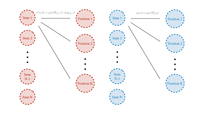
An alternative method (G-MLE) uses a greedy strategy, ranking items based on their MLE of user satisfaction score instead of the upper confidence bound. This strategy also forms a bipartite graph $G_{t}$, similar to $G^{U}_{t}$, but uses the MLE to assign edge weights: for each item $j\in s_{t}(X_{t})$ and each position $k\in[K]$, the weight $w_{t}(j,k)$ is given by $g_{k}(\hat{\mu}_{t,j}(k,X_{t}))$. A comparison of the bipartite graphs resulting from UCR and the MLE ranking is illustrated by Figure 3 in Appendix A. We shall compare the performance of UCR against G-MLE in Section 5, where G-MLE serves as a benchmark.

4 Main Result on Cumulative Regret

In this section, we present our main theoretical results on the cumulative regret guarantees using our algorithm. We highlight the key steps in our proof in Section 4.1 and defer the complete version to Appendix C.2.

Theorem 4.1.

Fix any $\delta\in(0,1)$, and let $c_{1}:=\min\{\frac{1}{2K},c_{x}\}>0$. Suppose Assumption 2.2 and 2.6 hold, and $T_{0}\geq\max\big{\{}(\frac{16}{3c_{1}}+\frac{32(K+N)^{2}}{N^{2}c_{1}})\log\frac{2(d+1)}{\delta},~{}\frac{6\bar{\sigma}^{2}}{c_{1}\kappa^{2}}((d+1)\log(1+2T/d)+\log(1/\delta))\big{\}}$. Then with probability at least $1-\delta$,

$$R_{T}\leq R_{0}T_{0}+\frac{5\bar{\sigma}}{\kappa}\cdot M_{1}\cdot\bar{c}\cdot d\sqrt{NKT}\log(T/(d\delta)),$$

where $\bar{c}=\max{k\in[K]}c_{k}$. With the proper choice of the initialization phase $T_{0}$,

$$R_{T}\leq\tilde{O}\bigg{(}\frac{(K+N)^{2}}{c_{1}}+\frac{\bar{\sigma}}{c_{1}\kappa^{2}}\cdot d+\frac{\bar{\sigma}}{\kappa}\cdot M_{1}\cdot\bar{c}\cdot d\sqrt{NKT}\bigg{)}.$$

Theorem 4.1 shows that the regret of our algorithm scales with $\sqrt{T}$, which is minimax optimal in standard contextual bandit results (Agrawal & Goyal, 2012; Chu et al., 2011). The factor $d$ is similar to the GLM bandit result in (Li et al., 2017). From the factor $\sqrt{NK}$, we see that our algorithm overcomes the combinatorial complexity of the ranking space (which is originally $\binom{N}{K}=\frac{N!}{K!(N-K)!}$ for choosing $K$ retrieved items from a total of $N$ items).

The regret bound in the special case $N=K$ is provided as Corollary 4.2. In this case, we obtain a slightly different constant factor $c_{H}=\sum_{k=1}^{K}c_{k}$ instead of $\sqrt{NK}\max_{k\in[K]}c_{k}$, because all items appear in the ranked list, and each item incurs an estimation error that enters the reget bound.

Corollary 4.2.

Let $N=K$. Fix any $\delta\in(0,1/2)$. Under Assumption, suppose $T_{0}\geq\max\big{\{}(\frac{32}{3c_{1}}+\frac{256}{c_{1}^{2}}\log(\frac{4d+4}{\delta}),~{}\frac{6\bar{\sigma}^{2}}{c_{1}\cdot\kappa^{2}}((d+1)\log(1+2T/d)+\log(2/\delta))\big{\}}$. Then

$\displaystyle R_{T}$ $\displaystyle\leq R_{0}T_{0}+\frac{5\bar{\sigma}}{\kappa}\cdot M_{1}\cdot c_{H}\cdot d\sqrt{T}\log(T/(d\delta))$

with probability at least $1-\delta$, where we denote $c_{H}:=\sum_{k=1}^{K}c_{k}$.

4.1 Proof sketch of Theorem 4.1

In this part, we lay out the proof sketch for Theorem 4.1. In a nutshell, our theory proceeds in three steps: (i) the random initialization of $T_{0}$ steps ensures that the covariance matrices ${V_{{j}}^{({t})}}$ are well-conditioned; (ii) the estimation error $\hat{\theta}_{t,j}-\theta_{j}$ is small once ${V_{{j}}^{({t})}}$ is well-conditioned; (iii) the cumulative regret is bounded in terms of the Lipschiz constant in the mean reward functions and the parameter estimation error. Among the three steps, (i) follows from standard concentration inequalities, which we defer to Lemma C.1 in Appendix C.2.

The key step (ii) is summarized in Proposition 4.3, which shows that with sufficiently many random initialization samples, the estimation errors later on can be uniformly bounded for all $t\geq T_{0}$. Our proof technique adapts that of (Li et al., 2017), and we include the detailed proofs in Appendix C.4.

Proposition 4.3.

For any $\delta\in(0,1)$. Let $c_{1}:=\min\{\frac{1}{2K},c_{x}\}>0$ and let

$\displaystyle T_{0}\geq\max\big{\{}$ $\displaystyle(\frac{16}{3c_{1}}+\frac{32(K+N)^{2}}{N^{2}c_{1}})\log\frac{2(d+1)}{\delta},$
$\displaystyle\frac{6\bar{\sigma}^{2}}{c_{1}\kappa^{2}}((d+1)\log(1+2T/d)+\log(1/\delta))\big{\}}.$

Then with probability at least $1-\delta$, for all $t\in[T_{0},T]$ and all $j\in[N]$, it holds that

$$\|\hat{\theta}_{t,j}-\theta_{j}\|_{V_{j}^{(t)}}\leq\frac{\sqrt{3}\bar{\sigma}}{\kappa}\sqrt{(d+1)\log(1+2T/d)+\log(1/\delta)}.$$

In step (iii), we bound the regret with the following lemma on the event that the estimation error $\hat{\theta}_{t,j}-\theta_{j}$ is uniformly small. Recall that $z_{\tau,j}=\big{(}\sigma_{\tau}\big{(}q_{\tau}^{-1}(j)\big{)},X_{\tau}\big{)}$ is the aggregated feature for item $j$ at time $\tau$. The proof of Lemma 4.4 is in Appendix C.5.

Lemma 4.4.

Denote

$$\xi=\frac{\sqrt{3}\bar{\sigma}}{\kappa}\sqrt{(d+1)\log(1+2T/d)+\log(2/\delta)}.$$

On the event of Proposition (4.3), it holds that

$$R_{T}\leq R_{T_{0}}+M_{1}\cdot 2\xi\cdot\sum_{t=T_{0}}^{T}\sum_{k=1}^{K}c_{k}\cdot\|Z_{t,q_{t}(k)}\|_{(V^{(t)}_{q_{t}(k)})^{-1}}.$$

In Lemma 4.4, the regret is split into $R_{T_{0}}$ (due to initial random initialization) and the estimation error. For the estimation error, each recommended item $q_{t}(k)\in s_{t}(X_{t})$ has regret bounded by its inverse-covariance-normalized feature norm, which can be further controlled via deterministic bounds on self-normalized norms (Abbasi-Yadkori et al., 2011).

Finally, we can conclude Theorem 4.1 by combing the results of Lemma C.1, 4.4 and Proposition 4.3. Observing the fact that on the event in Proposition 4.3, $\lambda_{\min}(V_{s}^{(T_{0})})\geq 1$ while $\|Z_{t,s}\|\leq 1$ for all time $t$ and item $s$, by a helper Lemma E.2, we derive the desired results. More details are in Appendix C.2.

Refer to caption
Refer to caption
Refer to caption
Figure 1: The average cumulative regret (with standard variation interval) of UCR and G-MLE in the simulated environment. The figure on the left is the result of the $N=7,K=5$ case; in the middle is the result of the $N=10,K=5$ case; the figure on the right is the result of the $N=K=5$ case.

Refer to caption

Figure 2: Average relative regret (with standard variation interval) of UCR and G-MLE on the real-world dataset.

5 Experiments

We hereby provide empirical performances of UCR and G-MLE (the comparison of which is in Remark 3.1) on a simulated dataset and a real-world dataset, with the goal of illuminating how the two algorithms perform across different environments. We note the inclusion of the real-world dataset to test our algorithm’s robustness and potential effectiveness in practical applications, as simulated environments often present idealized scenarios.

Simulated Environment: We evaluate the ranking algorithms on a generated environment, where the ground truth parameters are sampled as follows: the positional effects for each item are drawn uniformly from the interval $[0,1]$, and the contexts are drawn uniformly from a norm ball of a specified radius. We then perform ranking tasks within this generated environment. The detailed environment generation procedure is outlined in Algorithm 3 and 4 in Appendix A555The python code for executing the experiment can be found in https://github.com/arena-tools/ranking-agent.. We run the experiments under two main settings, one with $N>K$ and another with $N=K$. For the first setting, we includes two cases of $N=7,K=5$ and $N=10,K=5$. For the second setting, we let $N=K=5$.

Real-world Dataset: We test UCR and G-MLE using a real-world task, with the goal to maximize click-through rates of the company’s product recommendations 666For data-privacy reasons, the name of the company is not disclosed.. An offline dataset from the historical data, collected via a heuristics-based control policy, is used to learn a simulator. This simulator generates clicks for a given set of rankings, which are formulated as the reward in Algorithm 5 of Appendix A. The dataset comprises 13,717 samples and 436 unique items, all used for simulator training. Bootstrap samples are taken from a subset of 259 samples and $N=$114 items with positive rewards. Most features indicate if a user has recently purchased a similar item. The summary statistics of these features are in Table 1 of Appendix A. We run UCR and G-MLE with $K=3$ retrieved items and update each iteration with a batch size of 30 (each batch consists of 3 items), repeatedly for 200 runs.

5.1 Empirical Results

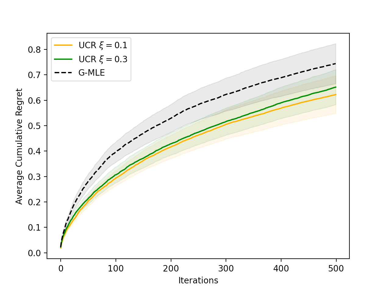
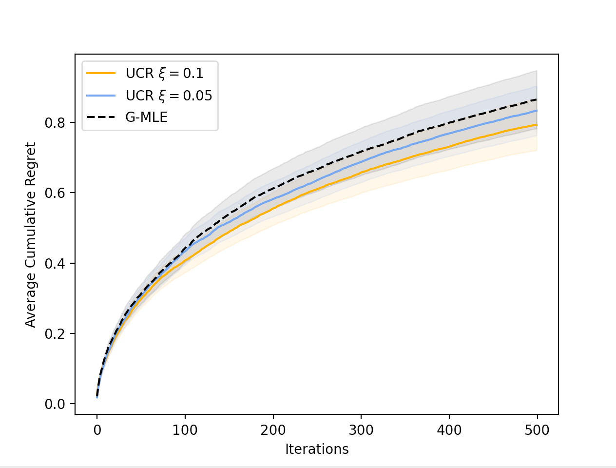
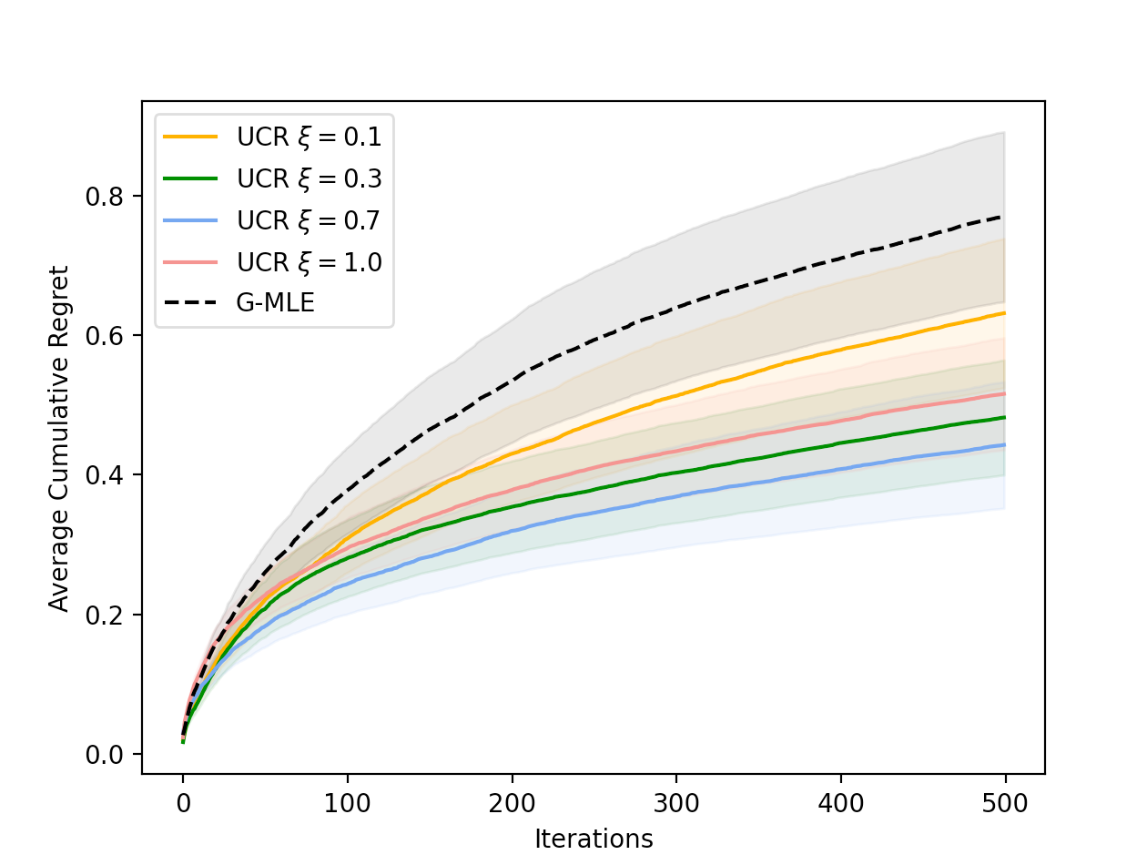
We present the empirical results of cumulative regrets on simulated dataset in Figure 1, over $T=500$ iterations and 300 runs. Additionally, we present the empirical results of the relative regrets on real-world dataset in Figure 2, over $T=100$ iterations and 200 runs. All experiments have a initialization phase $T_{0}=5$. For each setting we run several upper confidence parameters $\xi$ of UCR and present the regret curves of these instances along with those of the baseline G-MLE approach.

UCR consistently outperforms the G-MLE approach across different environments.

As shown in Figure 1, in both $N>K$ and $N=K$ settings, UCR yields lower average cumulative regret. These results also demonstrate the importance of choosing the right upper confidence parameter $\xi$. While UCR generally outperforms MLE, the advantage can shrink with poor choices of parameter $\xi$. Despite this, UCR still outperforms the baseline G-MLE in all settings and with all reasonably chosen $\xi$, showing the algorithm’s robustness.

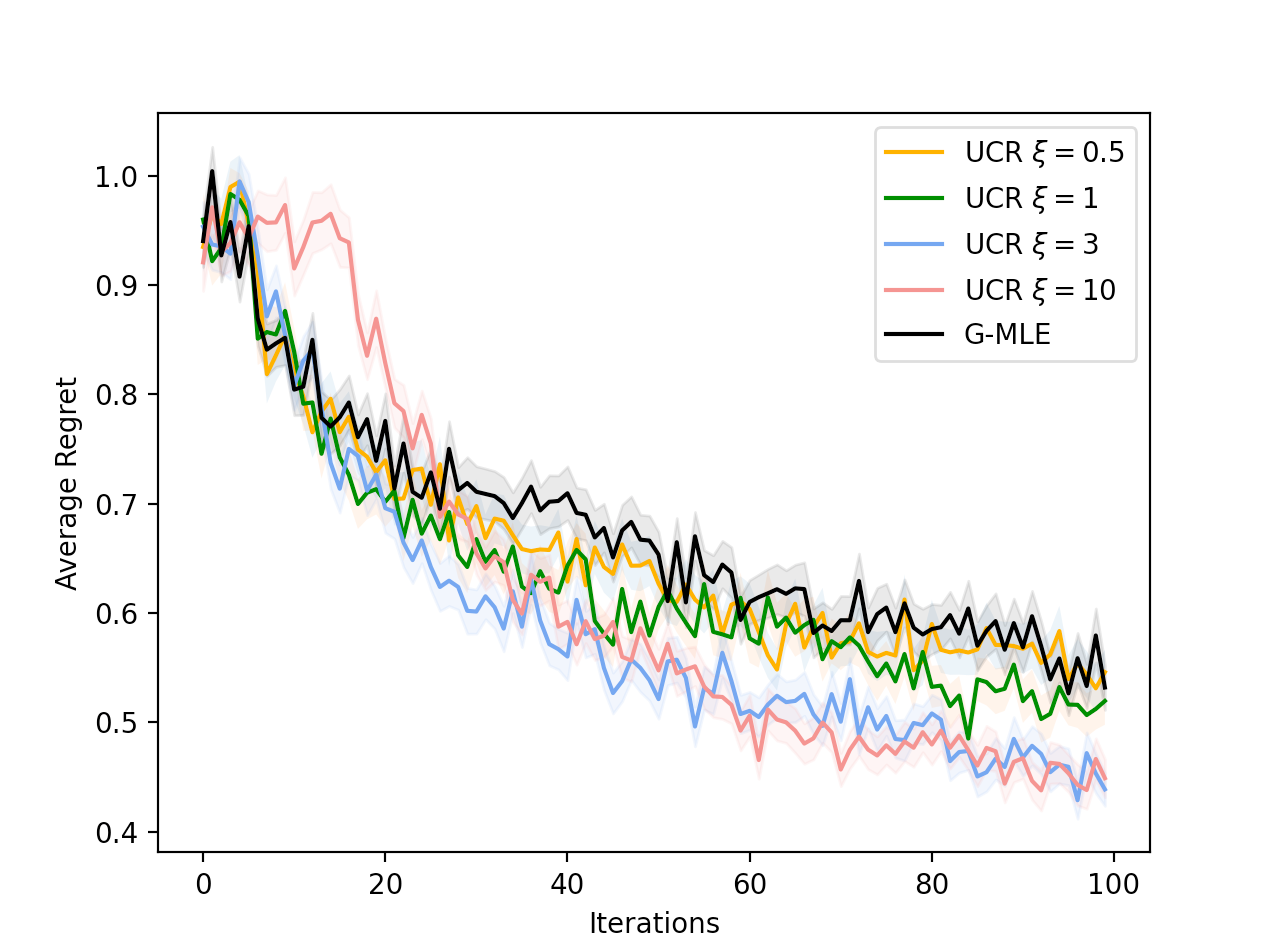
UCR maintains its advantage over G-MLE on real-world applications.

Figure 2 shows that the average relative regret of UCR on the real-world dataset is lower than that of the baseline MLE approach across all instances with various chosen hyperparameters $\xi$. Similarly as in the simulated environment experiment, we explore how the hyperparameter $\xi$ would affect the performance of UCR. Figure 2 indicates that poor choices of the hyperparameter $\xi$ could overcome the advantages of UCR over G-MLE. In this case, UCR with $\xi=0.5$ is comparable to G-MLE for large iterations; while lager $\xi$ results in smaller average relative regrets.

Overall, the results show that UCR not only outperforms G-MLE in a simulated environment but also in real-life applications, where the tasks inevitably contain more noise, and conclude the advantages of UCR further.

Acknowledgements

We cordially thank Pratap Ranade and Engin Ural for providing a world class environment at Arena that has helped shape and push an ambitious vision of this research agenda, where cutting edge active learning is finding its way to economic domains, for which this work is a specific instance.

Ruohan Zhan is partly supported by the Guangdong Provincial Key Laboratory of Mathematical Foundations for Artificial Intelligence (2023B1212010001) and the Project of Hetao Shenzhen-Hong Kong Science and Technology Innovation Cooperation Zone (HZQB-KCZYB-2020083). Zhengyuan Zhou also gratefully acknowledges the 2024 NYU CGEB faculty grant.

Impact Statement

This paper presents work whose goal is to advance the field of Machine Learning. There are many potential societal consequences of our work, none of which we feel must be specifically highlighted here.

References

  • (1) Google’s recommendation systems developer course. https://developers.google.com/machine-learning/recommendation. Accessed: 2023-05-14.
  • Abbasi-Yadkori et al. (2011) Abbasi-Yadkori, Y., Pál, D., and Szepesvári, C. Improved algorithms for linear stochastic bandits. In Advances in Neural Information Processing Systems, pp.  2312–2320, 2011.
  • Agichtein et al. (2006) Agichtein, E., Brill, E., and Dumais, S. Improving web search ranking by incorporating user behavior information. In Proceedings of the 29th annual international ACM SIGIR conference on Research and development in information retrieval, pp.  19–26, 2006.
  • Agrawal & Goyal (2012) Agrawal, S. and Goyal, N. Analysis of thompson sampling for the multi-armed bandit problem. In Conference on learning theory, pp.  39–1. JMLR Workshop and Conference Proceedings, 2012.
  • Agrawal et al. (2019) Agrawal, S., Avadhanula, V., Goyal, V., and Zeevi, A. Mnl-bandit: A dynamic learning approach to assortment selection. Operations Research, 67(5):1453–1485, 2019.
  • Auer et al. (2002) Auer, P., Cesa-Bianchi, N., and Fischer, P. Finite-time analysis of the multiarmed bandit problem. Machine learning, 47:235–256, 2002.
  • Bello et al. (2018) Bello, I., Kulkarni, S., Jain, S., Boutilier, C., Chi, E., Eban, E., Luo, X., Mackey, A., and Meshi, O. Seq2slate: Re-ranking and slate optimization with rnns. arXiv preprint arXiv:1810.02019, 2018.
  • Bennett et al. (2007) Bennett, J., Lanning, S., et al. The netflix prize. In Proceedings of KDD cup and workshop, volume 2007, pp.  35. New York, 2007.
  • Burges et al. (2005) Burges, C., Shaked, T., Renshaw, E., Lazier, A., Deeds, M., Hamilton, N., and Hullender, G. Learning to rank using gradient descent. In Proceedings of the 22nd international conference on Machine learning, pp.  89–96, 2005.
  • Burges (2010) Burges, C. J. From ranknet to lambdarank to lambdamart: An overview. Learning, 11(23-581):81, 2010.
  • Cao et al. (2007) Cao, Z., Qin, T., Liu, T.-Y., Tsai, M.-F., and Li, H. Learning to rank: from pairwise approach to listwise approach. In Proceedings of the 24th international conference on Machine learning, pp.  129–136, 2007.
  • Chen et al. (1999) Chen, K., Hu, I., and Ying, Z. Strong consistency of maximum quasi-likelihood estimators in generalized linear models with fixed and adaptive designs. The Annals of Statistics, 27(4):1155–1163, 1999.
  • Chen et al. (2019) Chen, M., Beutel, A., Covington, P., Jain, S., Belletti, F., and Chi, E. H. Top-k off-policy correction for a reinforce recommender system. In Proceedings of the Twelfth ACM International Conference on Web Search and Data Mining, pp.  456–464, 2019.
  • Chen et al. (2013) Chen, W., Wang, Y., and Yuan, Y. Combinatorial multi-armed bandit: General framework and applications. In International conference on machine learning, pp.  151–159. PMLR, 2013.
  • Chu et al. (2011) Chu, W., Li, L., Reyzin, L., and Schapire, R. Contextual bandits with linear payoff functions. In Proceedings of the Fourteenth International Conference on Artificial Intelligence and Statistics, pp.  208–214. JMLR Workshop and Conference Proceedings, 2011.
  • Chuklin et al. (2022) Chuklin, A., Markov, I., and De Rijke, M. Click models for web search. Springer Nature, 2022.
  • Collins et al. (2018) Collins, A., Tkaczyk, D., Aizawa, A., and Beel, J. A study of position bias in digital library recommender systems. arXiv preprint arXiv:1802.06565, 2018.
  • Combes et al. (2015) Combes, R., Talebi Mazraeh Shahi, M. S., Proutiere, A., et al. Combinatorial bandits revisited. Advances in neural information processing systems, 28, 2015.
  • Craswell et al. (2008) Craswell, N., Zoeter, O., Taylor, M., and Ramsey, B. An experimental comparison of click position-bias models. In Proceedings of the 2008 international conference on web search and data mining, pp.  87–94, 2008.
  • Freund et al. (2003) Freund, Y., Iyer, R., Schapire, R. E., and Singer, Y. An efficient boosting algorithm for combining preferences. Journal of machine learning research, 4(Nov):933–969, 2003.
  • Gauthier et al. (2022) Gauthier, C.-S., Gaudel, R., and Fromont, E. Unirank: Unimodal bandit algorithms for online ranking. In International Conference on Machine Learning, pp.  7279–7309. PMLR, 2022.
  • Guo et al. (2019) Guo, H., Yu, J., Liu, Q., Tang, R., and Zhang, Y. Pal: a position-bias aware learning framework for ctr prediction in live recommender systems. In Proceedings of the 13th ACM Conference on Recommender Systems, pp.  452–456, 2019.
  • Hamidi & Bayati (2020) Hamidi, N. and Bayati, M. A general theory of the stochastic linear bandit and its applications. arXiv preprint arXiv:2002.05152, 2020.
  • Herbrich et al. (1999) Herbrich, R., Graepel, T., and Obermayer, K. Support vector learning for ordinal regression. 1999.
  • Hu et al. (2008) Hu, Y., Koren, Y., and Volinsky, C. Collaborative filtering for implicit feedback datasets. In 2008 Eighth IEEE international conference on data mining, pp.  263–272. Ieee, 2008.
  • Joachims (2002) Joachims, T. Optimizing search engines using clickthrough data. In Proceedings of the eighth ACM SIGKDD international conference on Knowledge discovery and data mining, pp.  133–142, 2002.
  • Katariya et al. (2016) Katariya, S., Kveton, B., Szepesvari, C., and Wen, Z. Dcm bandits: Learning to rank with multiple clicks. In International Conference on Machine Learning, pp.  1215–1224. PMLR, 2016.
  • Komiyama et al. (2017) Komiyama, J., Honda, J., and Takeda, A. Position-based multiple-play bandit problem with unknown position bias. Advances in Neural Information Processing Systems, 30, 2017.
  • Kuhn (1955) Kuhn, H. W. The hungarian method for the assignment problem. Naval research logistics quarterly, 2(1-2):83–97, 1955.
  • Kveton et al. (2015) Kveton, B., Szepesvari, C., Wen, Z., and Ashkan, A. Cascading bandits: Learning to rank in the cascade model. In International conference on machine learning, pp.  767–776. PMLR, 2015.
  • Lagrée et al. (2016) Lagrée, P., Vernade, C., and Cappe, O. Multiple-play bandits in the position-based model. Advances in Neural Information Processing Systems, 29, 2016.
  • Lai et al. (1985) Lai, T. L., Robbins, H., et al. Asymptotically efficient adaptive allocation rules. Advances in applied mathematics, 6(1):4–22, 1985.
  • Lattimore et al. (2018) Lattimore, T., Kveton, B., Li, S., and Szepesvari, C. Toprank: A practical algorithm for online stochastic ranking. Advances in Neural Information Processing Systems, 31, 2018.
  • Lee & Lin (2014) Lee, C.-P. and Lin, C.-J. Large-scale linear ranksvm. Neural computation, 26(4):781–817, 2014.
  • Lerman & Hogg (2014) Lerman, K. and Hogg, T. Leveraging position bias to improve peer recommendation. PloS one, 9(6):e98914, 2014.
  • Li & Lin (2006) Li, L. and Lin, H.-T. Ordinal regression by extended binary classification. Advances in neural information processing systems, 19, 2006.
  • Li et al. (2017) Li, L., Lu, Y., and Zhou, D. Provably optimal algorithms for generalized linear contextual bandits. In International Conference on Machine Learning, pp.  2071–2080. PMLR, 2017.
  • Li et al. (2007) Li, P., Wu, Q., and Burges, C. Mcrank: Learning to rank using multiple classification and gradient boosting. Advances in neural information processing systems, 20, 2007.
  • Li et al. (2016) Li, S., Wang, B., Zhang, S., and Chen, W. Contextual combinatorial cascading bandits. In International conference on machine learning, pp.  1245–1253. PMLR, 2016.
  • Li et al. (2019) Li, S., Lattimore, T., and Szepesvári, C. Online learning to rank with features. In International Conference on Machine Learning, pp.  3856–3865. PMLR, 2019.
  • Lin et al. (2021) Lin, C., Liu, X., Xv, G., and Li, H. Mitigating sentiment bias for recommender systems. In Proceedings of the 44th International ACM SIGIR Conference on Research and Development in Information Retrieval, pp.  31–40, 2021.
  • Liu et al. (2009) Liu, T.-Y. et al. Learning to rank for information retrieval. Foundations and Trends® in Information Retrieval, 3(3):225–331, 2009.
  • McCullagh (2019) McCullagh, P. Generalized linear models. Routledge, 2019.
  • Qin et al. (2014) Qin, L., Chen, S., and Zhu, X. Contextual combinatorial bandit and its application on diversified online recommendation. In Proceedings of the 2014 SIAM International Conference on Data Mining, pp.  461–469. SIAM, 2014.
  • Ramshaw & Tarjan (2012) Ramshaw, L. and Tarjan, R. E. A weight-scaling algorithm for min-cost imperfect matchings in bipartite graphs. In 2012 IEEE 53rd Annual Symposium on Foundations of Computer Science, pp.  581–590. IEEE, 2012.
  • Russo et al. (2018) Russo, D. J., Van Roy, B., Kazerouni, A., Osband, I., Wen, Z., et al. A tutorial on thompson sampling. Foundations and Trends® in Machine Learning, 11(1):1–96, 2018.
  • Shidani et al. (2024) Shidani, A., Deligiannidis, G., and Doucet, A. Ranking in generalized linear bandits. In Workshop on Recommendation Ecosystems: Modeling, Optimization and Incentive Design, 2024.
  • Thompson (1933) Thompson, W. R. On the likelihood that one unknown probability exceeds another in view of the evidence of two samples. Biometrika, 25(3-4):285–294, 1933.
  • Tropp (2015) Tropp, J. A. An introduction to matrix concentration inequalities. Foundations and Trends in Machine Learning, 8(1–2):1–230, May 2015. ISSN 1935-8237. doi: 10.1561/2200000048.
  • Wang et al. (2019) Wang, F., Fang, X., Liu, L., Chen, Y., Tao, J., Peng, Z., Jin, C., and Tian, H. Sequential evaluation and generation framework for combinatorial recommender system. arXiv preprint arXiv:1902.00245, 2019.
  • Yao et al. (2021) Yao, S., Tan, J., Chen, X., Yang, K., Xiao, R., Deng, H., and Wan, X. Learning a product relevance model from click-through data in e-commerce. In Proceedings of the Web Conference 2021, pp.  2890–2899, 2021.
  • Ye et al. (2022) Ye, Z., Zhang, D. J., Zhang, H., Zhang, R., Chen, X., and Xu, Z. Cold start to improve market thickness on online advertising platforms: Data-driven algorithms and field experiments. Management Science, 2022.
  • Yu et al. (2023) Yu, Y., Jin, B., Song, J., Li, B., Zheng, Y., and Zhuo, W. Improving micro-video recommendation by controlling position bias. In Machine Learning and Knowledge Discovery in Databases: European Conference, ECML PKDD 2022, Grenoble, France, September 19–23, 2022, Proceedings, Part I, pp.  508–523. Springer, 2023.
  • Zhao et al. (2019) Zhao, Z., Hong, L., Wei, L., Chen, J., Nath, A., Andrews, S., Kumthekar, A., Sathiamoorthy, M., Yi, X., and Chi, E. Recommending what video to watch next: a multitask ranking system. In Proceedings of the 13th ACM Conference on Recommender Systems, pp.  43–51, 2019.
  • Zhong et al. (2021) Zhong, Z., Chueng, W. C., and Tan, V. Y. Thompson sampling algorithms for cascading bandits. The Journal of Machine Learning Research, 22(1):9915–9980, 2021.
  • Zhou et al. (2020) Zhou, D., Li, L., and Gu, Q. Neural contextual bandits with ucb-based exploration. In International Conference on Machine Learning, pp.  11492–11502. PMLR, 2020.
  • Zoghi et al. (2016) Zoghi, M., Tunys, T., Li, L., Jose, D., Chen, J., Chin, C. M., and de Rijke, M. Click-based hot fixes for underperforming torso queries. In Proceedings of the 39th International ACM SIGIR conference on Research and Development in Information Retrieval, pp.  195–204, 2016.
  • Zong et al. (2016) Zong, S., Ni, H., Sung, K., Ke, N. R., Wen, Z., and Kveton, B. Cascading bandits for large-scale recommendation problems. arXiv preprint arXiv:1603.05359, 2016.

Appendix A Additional Experiment Details

We shall introduce the details of the experiment. First of all, to better distinguish the bipartite matching schemes of UCR (our proposed algorithm) and G-MLE (the benchmark algorithm), we present the visualization of both in Figure 3.


Refer to caption

Figure 3: Visualization of Bipartite Matching of UCR and greedy MLE approach.

The details for how the simulated environment are listed below. We generate the ground truth simulator parameters following Algorithm 3, and for each step context is generated following Algorithm 4 from which the algorithm makes an update and predicts the probability of clicks. In our experiments, the context dimension is set to be $d=7$.

Algorithm 3 Generate simulator parameters
0:  number of items $N$, dimension of features $d$.
1:  for $n=1,\dots,N$ do
2:     $\alpha_{n}\leftarrow\mbox{Uniform}[0,1].$
3:     $\beta_{n}\leftarrow\mbox{Uniform}(\mathcal{B}(1,\mathbb{R}^{d}))$.
4:  end for
4:  position effect $\{\alpha_{n}\}_{n=1}^{N}$, item features $\{\beta_{n}\}_{n=1}^{N}$.
Algorithm 4 Generate context
0:  Context dimension $d$.
1:  $x\leftarrow\mbox{Uniform}(\mathcal{B}(1,\mathbb{R}^{d}))$.
1:  $x$.

The details for the construction of the real-world experiment are as follows. We first provide the summary statistics for the real-world dataset used in our experiments in Table 1. All features except Store Type are binary features indicating if the user has purchased the same type of item recently.

Table 1: Summary Statistics for Offline Dataset
Features Description p-Value
Store Type Represents the type of store making the purchase of the drink 0
Item Indicated if the user recently purchased the same item 0
Liquid Indicates if the user recently purchased the same liquid type 0.792
Style Indicates if the user recently purchased same style of items 0.005
Brand Indicates if the user recently purchased the same brand of items 0.177
Container Indicates if the user recently purchased any items of the same container type 0.008
Material Indicates if the user recently purchased any items of the same container material 0.489
Case Indicates if the user recently purchased any items of the same container case configuration 0.684

We simulate the reward under this setting as occurrence of clicks, which is outputted by the model as in Algorithm 5.

Algorithm 5 Generate click occurrence
0:  true environment $\{(\alpha_{k},\beta_{k})\}_{k=1}^{K}$, context $x$, ranking $\sigma$.
1:  for $k=1,\dots,K$ do
2:     Sampling probability $p_{k}=\frac{1}{\exp(\alpha_{k}\sigma(k)-x^{T}\beta_{k})}$.
3:     Click $Y_{k}\sim\mbox{Bernoulli}(p_{k})$
4:  end for
4:  Clicks for $K$ items $\{Y_{k}\}_{k=1}^{K}$.

Appendix B Extension to Feature-Based Ranking

The UCR algorithm can be extended to perform feature-based ranking by making the model only dependent on user and product features, which allows the UCR ranking algorithm to learn the effects of interactions between the user and product and rank without prefiltering and rank an arbitrary set of items with only a single ranking model. Model the probability of clicks as

$\displaystyle\mathbb{P}(Y_{t,j,k}=1{\,|\,}X_{t};\alpha_{j},\beta_{j})=\mathbb{E}[Y_{t,j,k}|X_{t};\alpha_{j},\beta_{j}]=\big{(}1+e^{-\vec{z}^{T}(k)\vec{\theta}})^{-1}.$

$\vec{\theta}=[-\alpha_{1},\alpha_{2}^{T},\alpha_{3}^{T},w_{11},w_{12},...,w_{mn}]^{T}$ is the feature vector representing each of the product and user features and flattened correlation matrix $W$.

$\vec{z}(k)=[\sigma_{i}(k),\vec{x_{i}},\vec{y_{i}},\vec{x}_{i}\times\vec{y}_{i}]$ where $\vec{x}_{i}\times\vec{y}_{i}$ is the flattened Cartesian product of the product and user vectors at step $i$ and $\sigma_{i}(k)$ is the rank of item $k$ at step $i$

Then, the UCB probability can be expressed as $p(k,i)=\{1+\exp(-\alpha_{1}\sigma_{i}(k)+\alpha_{2}^{T}x_{i}+\alpha_{3}^{T}y_{i}+x^{T}_{i}Wy_{i}-3\xi\sqrt{z^{T}V^{-1}z}\}^{-1},z=(i,\vec{x_{i}},\vec{y_{i}},\vec{x}_{i}\times\vec{y}_{i}).$

The solution can be obtained by solving the matching problem for the bipartite graph in the same way as stated in Algorithm 2.

Appendix C Omitted Technical Proofs

C.1 Derivation of Equation (2)

Denote the log-likelihood function $l(X_{t},\beta_{j},\alpha_{j};y)=\log f_{Y_{t,j,k}\mid X_{t};\beta_{j},\alpha_{j}}(y)$ as a function of $(X_{t};\beta_{j},\alpha_{j})$ and $y$. The mean of $Y_{t,j,k}\mid X_{t};\beta_{j},\alpha_{j}$ can be derived from the known relations of exponential family: $\mathbb{E}[\frac{\partial l(X_{t},\beta_{j},\alpha_{j};y)}{\partial(\alpha_{j}k+\beta_{j}^{T}X_{t})}]=0$. Define $\hat{h}(Y_{t,j,k},\tau)=\exp(h(Y_{t,j,k},\tau))$, we have that

$\displaystyle l(X_{t},\beta_{j},\alpha_{j};y)=\frac{y(\alpha_{j}k+\beta_{j}^{T}X_{t})-A(\alpha_{j}k+\beta_{j}^{T}X_{t})}{d(\tau)}+\hat{h}(y,\tau),$

and therefore

$\displaystyle\frac{\partial l(X_{t},\beta_{j},\alpha_{j};y)}{\partial(\alpha_{j}k+\beta_{j}^{T}X_{t})}=\frac{y-A^{\prime}(\alpha_{j}k+\beta_{j}^{T}X_{t})}{d(\tau)}.$

Plugin the result back into $\mathbb{E}[\frac{\partial l(X_{t},\beta_{j},\alpha_{j};y)}{\partial(\alpha_{j}k+\beta_{j}^{T}X_{t})}]$, we have that

$\displaystyle 0=\mathbb{E}[\frac{\partial l(X_{t},\beta_{j},\alpha_{j};y)}{\partial(\alpha_{j}k+\beta_{j}^{T}X_{t})}]=\frac{\mathbb{E}[Y_{t,j,k}\mid X_{t};j,k]-A^{\prime}(\alpha_{j}k+\beta_{j}^{T}X_{t})}{d(\tau)},$

hence

$\displaystyle\mathbb{E}[Y_{t,j,k}\mid X_{t};j,k]=A^{\prime}(\alpha_{j}k+\beta_{j}^{T}X_{t}).$

For more details, please refer to (McCullagh, 2019).

C.2 Proof of Theorem 4.1

Proof of Theorem 4.1.

Step (i) in our proof sketch is in Lemma C.1, whose proof is in Appendix C.3.

Lemma C.1.

Fix any $\delta\in(0,1)$, and let $c_{1}:=\min\{\frac{1}{2K},c_{x}\}$ and $B>0$ be any positive constant. Suppose $T_{0}\geq\max\{(\frac{16}{3c_{1}}+\frac{32(K+N)^{2}}{N^{2}c_{1}})\log\frac{2(d+1)}{\delta},\frac{2B}{c_{1}}\}$, then with probability at least $1-\delta$, we have $\lambda_{\min}(V_{j}^{(t)})\geq B$ for all $t\geq T_{0}$ and all $j\in[N]$.

Let $k_{t,j}$ be the position assigned to item $j$ at $t$ if item $j$ is included in the recommended list. Then following the upper bound in Lemma 4.4, we have

$\displaystyle R_{T}-R_{T_{0}}\leq\sum_{t=T_{0}}^{T}\sum_{j=1}^{N}\operatorname{\mathds{1}}\{j\in s_{t}(X_{t})\}\cdot c_{k_{t,j}}\cdot\|Z_{t,j}\|_{(V^{(t)}_{j})^{-1}}\leq\bar{c}\cdot\sum_{j=1}^{N}\sum_{t\in{\mathcal{T}}_{j},t\geq T_{0}}\|Z_{t,j}\|_{(V_{j}^{(t)})^{-1}},$

where $\bar{c}=\max_{k}c_{k}$. We then use the self-normalized concentration inequality (c.f. Lemma E.2) to bound $\sum_{t\in{\mathcal{T}}_{j},t\geq T_{0}}\|Z_{t,j}\|_{(V_{j}^{(t)})^{-1}}$. Under the notations of Lemma E.2, fixing any $j\in[N]$, we let $\bar{\mathcal{T}}_{j}=\{s\colon s\in{\mathcal{T}}_{j},s\geq T_{0}\}=\{s_{j,1},s_{j,2},\dots,s_{j,|\bar{\mathcal{T}}_{j}|}\}$; that is, $s_{j,t}$ is the $t$-th time after $T_{0}$ that item $j$ appears in the recommended list. Then setting $X_{t}=Z_{s_{j,t},j}$, $V=V_{j}^{(T_{0})}$, we note that $\bar{V}_{t}:=V_{j}^{(s_{j,t})}=V+\sum_{i=1}^{t}X_{s_{j,t}}X_{s_{j,t}}^{\top}$. Also, on the event in Proposition 4.3 we see $\lambda_{\min}(V_{s}^{(T_{0})})\geq 1$ while $\|Z_{t,s}\|\leq 1$. Thus, invoking Lemma E.2, we have

$\displaystyle\sum_{t\in{\mathcal{T}}_{j},t\geq T_{0}}\|Z_{t,j}\|_{(V^{(t)}_{j})^{-1}}$ $\displaystyle\leq 2\log\bigg{(}\frac{\det(V_{j}^{(T)})}{\det(V_{j}^{(T_{0})})}\bigg{)}$
$\displaystyle\leq 2d\log\bigg{(}\frac{\mathop{\mathrm{tr}}(V)+|\bar{\mathcal{T}}_{j}|}{d}\bigg{)}-2\log\det V_{j}^{(T_{0})},$

where $\mathop{\mathrm{tr}}(V)\leq\sum_{i=1}^{T_{0}}\mathop{\mathrm{tr}}(Z_{i,j}Z_{i,j}^{\top})\leq T_{0}$, and $\det(V_{j}^{(T_{0}+1)})\geq 1$ since $\lambda_{\min}(V_{j}^{(T_{0}+1)})\geq\lambda_{\min}(V_{j}^{(T_{0})})\geq 1$. Therefore, by the Cauchy-Schwarz inequality, we have

$$\sum_{t\in{\mathcal{T}}_{j},t\geq T_{0}}\|Z_{t,j}\|_{(V^{(t)}_{j})^{-1}}\leq\bigg{(}|\bar{\mathcal{T}}_{j}|\sum_{t\in{\mathcal{T}}_{j},t\geq T_{0}}\|Z_{t,j}\|_{(V_{j}^{(t)})^{-1}}^{2}\bigg{)}^{1/2}\leq\sqrt{|\bar{\mathcal{T}}_{j}|}\cdot\sqrt{2d\log(T/d)}$$

simultaneously for all $s\in[K]$ on the events in Proposition 4.3. Since $|\bar{\mathcal{T}}_{j}|\leq|{\mathcal{T}}_{j}|$, this further implies

$\displaystyle R_{T}$ $\displaystyle\leq R_{T_{0}}+2\xi\cdot M_{1}\cdot\bar{c}\sum_{j=1}^{N}\sqrt{|{\mathcal{T}}_{j}|}\cdot\sqrt{2d\log(T/d)}$
$\displaystyle\leq R_{T_{0}}+2\xi\cdot M_{1}\cdot\bar{c}\cdot\sqrt{N}\cdot\sqrt{\sum_{j=1}^{N}|{\mathcal{T}}_{j}|}\cdot\sqrt{2d\log(T/d)}$
$\displaystyle\leq R_{T_{0}}+2\xi\cdot M_{1}\cdot\bar{c}\cdot\sqrt{NKT}\cdot\sqrt{2d\log(T/d)}$
$\displaystyle\leq R_{T_{0}}+\frac{2\sqrt{3}\bar{\sigma}}{\kappa}\cdot M_{1}\cdot\bar{c}\cdot\sqrt{NKT}\cdot\sqrt{(d+1)\log(1+2T/d)+\log(2/\delta)}\cdot\sqrt{2d\log(T/d)}$
$\displaystyle\leq R_{0}T_{0}+\frac{5\sigma}{\kappa}\cdot M_{1}\cdot\bar{c}\cdot d\sqrt{NKT}\log(T/(d\delta))$

with probability at least $1-\delta$. Above, the second line uses the Cauchy-Schwarz inequality, and the third line uses the fact that $\sum_{i=1}^{N}|{\mathcal{T}}_{j}|=\sum_{i=1}^{N}\sum_{t=1}^{T}\operatorname{\mathds{1}}\{j\in s_{t}(X_{t})\}=\sum_{t=1}^{T}|s_{t}(X_{t})|=KT$. We thus conclude the proof. ∎

C.3 Proof of Lemma C.1

Proof.

By the definition of $V_{j}^{(t)}$, for any $t\geq T_{0}$, we have

$$V_{j}^{(t)}=V_{j}^{(T_{0})}+\sum_{i=T_{0}}^{t-1}z_{j}^{(i)}(z_{j}^{(i)})^{\top}\succeq V_{j}^{(T_{0})}.$$

Hence $\lambda_{\min}(V_{j}^{(t)})\geq\lambda_{\min}(V_{j}^{(T_{0})})$. It suffices to bound $\lambda_{\min}(V_{j}^{T_{0}})$ simultaneously for all $j\in[N]$. Consider the distribution of

$$V_{j}^{(T_{0})}=\sum_{t=1}^{T_{0}-1}\mathbbm{1}\{j\in(X_{t})\}Z_{t,j}(Z_{t,j})^{\top}.$$

Due to the random sampling of $s_{t}(X_{t})$ for all $t<T_{0}$, the matrix $V_{j}^{T_{0}}$ are summations of i.i.d. matrices with expectation

$\displaystyle\Sigma_{j}:=\mathbb{E}[\mathbbm{1}\{j\in(X_{t})\}Z_{t,j}(Z_{t,j})^{\top}]=\frac{K}{N}\mathbb{E}[Z_{t,j}(Z_{t,j})^{\top}],$

where

$\displaystyle\mathbb{E}[Z_{t,j}(Z_{t,j})^{\top}]=\begin{pmatrix}\mathbb{E}[\text{Unif}(-\frac{1}{2}+\frac{1}{K},-\frac{1}{2}+\frac{2}{K},\cdots,\frac{1}{2})]&0\\ 0&\mathbb{E}[X_{t}X_{t}^{\top}]\end{pmatrix}=\begin{pmatrix}\frac{1}{2K}&0\\ 0&\Sigma_{x,j}\end{pmatrix}.$

Note that $(Z_{t,j})=(\sigma_{t}(j),X_{t})$, and since $\sigma_{t}(j)$’s are rescaled, they follow Unif$(-\frac{1}{2}+\frac{1}{K},-\frac{1}{2}+\frac{2}{K},\cdots,\frac{1}{2})$. By the independence of $\sigma_{t}(j)$ and $X_{t}$, we derive the above result.

Hence $\lambda_{\min}(\Sigma_{j})\geq\min\{\frac{1}{2K},\lambda_{\min}(\Sigma_{x,j})\}\geq c_{1}:=\min\{\frac{1}{2K},c_{x}\}$, where $\lambda_{\min}(\Sigma_{x,j})\geq c_{x}$. By Jensen’s inequality, we have $\|\Sigma_{j}\|_{op}=\frac{K}{N}\|\mathbb{E}[Z_{t,j}(Z_{t,j})^{\top}]\|_{op}\leq\frac{K}{N}\mathbb{E}[\|Z_{t,j}\|^{2}]\leq\frac{K}{N}$. By the independence of each ranking before $T_{0}$, the random matrices $\{z_{t,j}(z_{t,j})^{\top}-\Sigma_{j}\}_{t=1}^{T_{0}-1}$ are i.i.d. centered in $\mathbb{R}^{(d+1)\times(d+1)}$ with uniformly bounded matrix operator norm:

$$\|z_{t,j}(z_{t,j})^{\top}-\Sigma_{j}\|_{op}\leq\|z_{t,j}(z_{t,j})^{\top}\|+\|\Sigma_{j}\|_{op}=1+\frac{K}{N}=\frac{K+N}{N}.$$

Now, define $\bar{V}_{j}:=V_{j}^{(T_{0})}-T_{0}\Sigma_{j}=\sum_{t=1}^{T_{0}-1}\{z_{t,j}(z_{t,j})^{\top}-\Sigma_{j}\}$. By triangle inequality,

$\displaystyle\|\mathbb{E}[\bar{V}_{j}\bar{V}_{j}^{\top}]\|_{op}=$ $\displaystyle\bigg{\|}\sum_{t=1}^{T_{0}-1}\mathbb{E}[\{z_{t,j}(z_{t,j})^{\top}-\Sigma_{j}\}\{z_{t,j}(z_{t,j})^{\top}-\Sigma_{j}\}^{\top}]\bigg{\|}_{op}$
$\displaystyle\leq$ $\displaystyle T_{0}\cdot\|\mathbb{E}[\{z_{t,j}(z_{t,j})^{\top}-\Sigma_{j}\}\{z_{t,j}(z_{t,j})^{\top}-\Sigma_{j}\}^{\top}]\|_{op}$
$\displaystyle\leq$ $\displaystyle T_{0}\cdot\mathbb{E}\|\{z_{t,j}(z_{t,j})^{\top}-\Sigma_{j}\}\{z_{t,j}(z_{t,j})^{\top}-\Sigma_{j}\}^{\top}\|_{op}$
$\displaystyle\leq$ $\displaystyle T_{0}\cdot\mathbb{E}\|z_{t,j}(z_{t,j})^{\top}-\Sigma_{j}\|_{op}\|z_{t,j}(z_{t,j})^{\top}-\Sigma_{j}\}^{\top}\|_{op}\leq T_{0}\bigg{(}\frac{K+N}{N}\bigg{)}^{2}.$

Similarly $\|\mathbb{E}[\bar{V}_{j}^{\top}\bar{V}_{j}]\|_{op}\leq T_{0}\frac{K+N}{N}$. Then by the matrix Bernstein’s inequality, for any $t\geq 0$:

$$\mathbb{P}(\|\bar{V}_{j}\|_{op}\geq t)\leq 2(d+1)\cdot\exp\bigg{(}-\frac{\frac{t^{2}}{2}}{T_{0}(\frac{K+N}{N})^{2}+\frac{2t}{3}}\bigg{)}.$$

The right-handed side is not greater than $\delta$ for any $t$ such that $t\geq\sqrt{2T_{0}(\frac{K+N}{N})^{2}\log\frac{2(d+1)}{\delta}}$ and $t\geq\frac{4}{3}\log\frac{2(d+1)}{\delta}$. Thus, with probability at least $1-\delta$, we have

$$\|\bar{V}_{j}^{(T_{0})}-T_{0}\Sigma_{j}\|_{op}\leq\sqrt{2T_{0}\bigg{(}\frac{K+N}{N}\bigg{)}^{2}\log\frac{2(d+1)}{\delta}}+\frac{4}{3}\log\frac{2(d+1)}{\delta},$$

and hence

$$\lambda_{\min}(V_{j}^{T_{0}})\geq T_{0}\cdot\lambda_{\min}(\Sigma_{j})-\sqrt{2T_{0}\bigg{(}\frac{K+N}{N}\bigg{)}^{2}\log\frac{2(d+1)}{\delta}}-\frac{4}{3}\log\frac{2(d+1)}{\delta}.$$

This implies that

$$\lambda_{\min}(V_{j}^{T_{0}})\geq T_{0}/2\cdot\lambda_{\min}(\Sigma_{j}),$$

as long as $\sqrt{2T_{0}(\frac{K+N}{N})^{2}\log\frac{2(d+1)}{\delta}}\leq T_{0}/4\cdot\lambda_{\min}(\Sigma_{j})$ and $\frac{4}{3}\log\frac{2(d+1)}{\delta}\leq T_{0}/4\cdot\lambda_{\min}(\Sigma_{j})$. Setting $T_{0}\geq(\frac{16}{3c_{1}}+\frac{32(K+N)^{2}}{N^{2}c_{1}})\log\frac{2(d+1)}{\delta}$, we have

$$\lambda_{\min}(V_{j}^{T_{0}})\geq T_{0}c_{1}/2$$

with probability at least $1-\delta$. Further let $T_{0}\geq\max\{(\frac{16}{3c_{1}}+\frac{32(K+N)^{2}}{N^{2}c_{1}})\log\frac{2(d+1)}{\delta},\frac{2B}{c_{1}}\}$, we have $\lambda_{\min}(V_{j}^{(T_{0})})\geq B$ with probability at least $1-\delta$. ∎

C.4 Proof of Proposition 4.3

Proof of Proposition 4.3.

Fix any $j\in[N]$. Throughout the proof, we condition on $\{X_{i}\}_{i=1}^{T}$, and define the martingale $\{\mathcal{H}_{\tau,j}\}_{\tau=0}^{T}$, where

$\displaystyle\mathcal{H}_{\tau,j}=\sigma\big{(}\{Z_{1,i},Y_{1,i},\cdots,Z_{\tau-1,i},Y_{\tau-1,i},Z_{\tau,i}\}_{i=1}^{n}\big{)}$

is the history of all rewards $Y_{t,i}$ for items that appeared in the recommended lists up to time $\tau-1$, and the ranking decisions $Z_{\tau,i}$ up to time $\tau$. We slightly deviate from the notation in the main text and use $Y_{t,i}$ for ease of presentation. Here without loss of generality, we impose $Y_{t,i}=0$ and $Z_{t,i}=0$ if $i\notin s_{t}(X_{t})$. For any $t\geq 1$, we define

$\displaystyle{\mathcal{T}}_{t}^{(j)}=\{\tau\leq t-1\colon j\in s(X_{\tau})\}$

be the set of time steps where item $j$ appears in the recommended list.

For any $t\in[T]$ and $j\in[N]$, we define

$\displaystyle L_{t,j}(\theta)=\sum_{\tau\in\mathcal{T}_{t}^{(j)}}Y_{\tau,j}\theta^{\top}Z_{\tau,j}-A(\theta^{\top}Z_{\tau,j}),\quad\nabla L_{t,j}(\theta)=\sum_{\tau\in\mathcal{T}_{t}^{(j)}}Y_{\tau,j}Z_{\tau,j}-A^{\prime}(\theta^{\top}Z_{\tau,j})Z_{\tau,j}.$

By the first-order condition of the MLE for $\hat{\theta}_{t,j}$, we have $\nabla L_{t,j}(\hat{\theta}_{t,j})=0$, and

$\displaystyle\nabla L_{t,j}(\theta_{j})=\sum_{\tau\in\mathcal{T}_{t}^{(j)}}Z_{\tau,j}\big{(}Y_{\tau,j}-A^{\prime}(\theta_{j}^{\top}Z_{\tau,j})\big{)}:=\sum_{\tau\in\mathcal{T}_{t}^{(j)}}Z_{\tau,j}\epsilon_{\tau,j},$

where $\epsilon_{\tau,j}:=Y_{\tau,j}-A^{\prime}(\theta_{j}^{\top}Z_{\tau,j})$ obeys $\mathbb{E}[\epsilon_{\tau,j}{\,|\,}\mathcal{H}_{\tau,j}]=0$ due to our models. By the mean value theorem, there exists some $\tilde{\theta}_{t,j}$ that lies on the segment between $\theta_{j}$ and $\hat{\theta}_{t,j}$, such that

$\displaystyle\sum_{\tau=1}^{t-1}Z_{\tau,j}\epsilon_{\tau,j}=\nabla L_{t,j}(\theta_{j})-\nabla L_{t,j}(\hat{\theta}_{t,j})=\nabla^{2}L_{t,j}(\tilde{\theta}_{t,k})(\theta_{j}-\hat{\theta}_{t,j}),$

where $\nabla^{2}L_{\tau,j}(\theta)$ is the Hessian matrix of $L_{\tau,j}$ at $\theta$. That is,

$\displaystyle\sum_{\tau=1}^{t-1}Z_{\tau,j}\epsilon_{\tau,j}=\sum_{\tau=1}^{t-1}A^{\prime\prime}(\tilde{\theta}_{t,j}^{\top}Z_{\tau,j})Z_{\tau,j}Z_{\tau,j}^{\top}(\theta_{j}-\hat{\theta}_{t,j}).$

Recalling (ii) $\kappa:=\inf_{\|z\|\leq 1,\|\theta-\theta_{k}\|\leq 1}{A^{\prime\prime}}(\theta^{\top}z)>0$ in Assumption 2.6(b), and noting that $V_{j}^{(t)}=\sum_{\tau=1}^{t-1}Z_{\tau,j}Z_{\tau,j}^{\top}$, we know that

$\displaystyle\Big{\|}\sum_{\tau=1}^{t-1}Z_{\tau,j}\epsilon_{\tau,j}\Big{\|}_{(V_{j}^{(t)})^{-1}}^{2}\geq\kappa^{2}\|\hat{\theta}_{t,j}-\theta_{k}\|_{V_{j}^{(t)}}^{2}$ (9)

holds as long as $\|\hat{\theta}_{t,j}-\theta_{j}\|_{2}\leq 1$.

In the sequel, we are to show that $\|\hat{\theta}_{t,j}-\theta_{j}\|_{2}\leq 1$ with high probability. Let

$\displaystyle S_{t,j}(\theta)=\nabla L_{t,j}(\theta_{j})-\nabla L_{t,j}(\theta)=\sum_{\tau\in\mathcal{T}_{t}^{(j)}}\big{(}A^{\prime}(\theta_{j}^{\top}Z_{\tau,j})-A^{\prime}(\theta^{\top}Z_{\tau,j})\big{)}Z_{\tau,j}.$

Note that $A^{\prime}$ is increasing, hence $A^{\prime\prime}(\cdot)>0$. Also, as long as $V_{j}^{(t)}>0$, we know that $S_{t,j}(\theta)$ is strictly convex in $\theta\in\mathbb{R}^{d+1}$, and thus $S_{t,j}$ is an injection from $\mathbb{R}^{d+1}$ to $\mathbb{R}^{d+1}$. Furthermore, for any $\theta$ with $\|\theta-\theta_{j}\|\leq 1$, there exists some $\tilde{\theta}$ that lies on the segment between $\theta$ and $\theta_{j}$ such that

$\displaystyle\|S_{t,j}(\theta)\|_{(V_{j}^{(t)})^{-1}}^{2}=\Big{\|}\sum_{\tau=1}^{t-1}A^{\prime\prime}(\tilde{\theta}^{\top}Z_{\tau,j})Z_{\tau,j}Z_{\tau,j}^{\top}(\theta_{j}-\theta)\Big{\|}_{(V_{j}^{(t)})^{-1}}^{2}\geq\kappa^{2}\lambda_{\min}(V_{j}^{(t)})\|\theta_{j}-\theta\|^{2}.$

The above arguments verify the conditions needed in Chen et al. (1999, Lemma A); it then implies for any $r>0$,

$\displaystyle\Big{\{}\theta\colon\|S_{t,j}(\theta)\|_{(V_{j}^{(t)})^{-1}}^{2}\leq\kappa^{2}r^{2}{\lambda_{\min}(V_{j}^{(t)})}\Big{\}}\subseteq\{\theta\colon\|\theta-\theta_{j}\|\leq r\}.$ (10)

Note that (10) is a deterministic result. Recall that $S_{t,j}(\hat{\theta}_{t,j})=\sum_{\tau\in\mathcal{T}_{t}^{(j)}}Z_{\tau,j}\epsilon_{\tau,j}$, and $\epsilon_{\tau,j}$ are mean-zero conditional on $\mathcal{H}_{\tau,j}$. We now use a more coarse martingale

$\displaystyle\mathcal{H}_{i,j}^{0}=\mathcal{H}_{\tau_{i,j},j},$

where $\tau_{i,j}$ is the $i$-th time that $j$ appears in $s_{t}(X_{t})$; put differently, $\tau_{i,j}$ is the $i$-th smallest member in $\mathcal{T}_{T}^{(j)}$. We know that for any $\tau=\tau_{i,j}$ for any $i\leq|{\mathcal{T}}_{t}^{(j)}|$, we still have $\mathbb{E}[\epsilon_{\tau,j}{\,|\,}\mathcal{H}_{i,j}^{0}]=0$ due to the fact that $\mathbb{E}[\epsilon_{\tau,j}{\,|\,}\mathcal{H}_{\tau,j}]=0$ we discussed before. Therefore, we can invoke the concentration inequality of self-normalized processes in Lemma E.3 for

$\displaystyle\sum_{\tau\in\mathcal{T}_{t}^{(j)}}Z_{\tau,j}\epsilon_{\tau,j}=\sum_{i=1}^{|\mathcal{T}_{t}^{(j)}|}Z_{\tau_{i,j},j}\epsilon_{\tau_{i,j},j}\quad\textrm{and}\quad\bar{V}_{t,j}:=\lambda I+\sum_{\tau\in\mathcal{T}_{t}^{(j)}}Z_{\tau,j}Z_{\tau,j}^{\top}=\lambda I+\sum_{i=1}^{|\mathcal{T}_{t}^{(j)}|}Z_{\tau_{i,j},j}Z_{\tau_{i,j},j}^{\top}$

for some fixed $\lambda>0$, which yields that with probability at least $1-\delta$, it holds for all $t\geq 1$ that

$\displaystyle\Big{\|}\sum_{\tau\in\mathcal{T}_{t}^{(j)}}Z_{\tau,j}\epsilon_{\tau,j}\Big{\|}_{\bar{V}_{t,j}^{-1}}^{2}\leq 2\bar{\sigma}^{2}\log\Bigg{(}\frac{\det(\bar{V}_{t,j})^{1/2}\det(\lambda I)^{-1/2}}{\delta}\Bigg{)}.$

Note that $\det(\lambda I)=\lambda^{d+1}$, and $\det(\bar{V}_{t,j})\leq(\lambda_{\max}(\bar{V}_{t,j}))\leq(\lambda+|\mathcal{T}_{t}^{(j)}|/d)^{d+1}$ since $\|Z_{\tau,j}\|_{2}\leq 1$ by Lemma E.4. We then have

$\displaystyle\Big{\|}\sum_{\tau\in\mathcal{T}_{t}^{(j)}}Z_{\tau,j}\epsilon_{\tau,j}\Big{\|}_{\bar{V}_{t,j}^{-1}}^{2}\leq 2\bar{\sigma}^{2}\big{(}(d+1)\log(1+|\mathcal{T}_{t}^{(j)}|/(d\lambda))+\log(1/\delta)\big{)}$ (11)

with probability at least $1-\delta$ for all $t\geq 1$.

By Lemma C.1, we know that

$\displaystyle\lambda_{\min}(V_{j}^{(t)})\geq\frac{3\bar{\sigma}^{2}}{\kappa^{2}}\big{(}(d+1)\log(1+2t/d)+\log(1/\delta)\big{)}$ (12)

holds with probability at least $1-\delta$ since $T_{0}\geq\max\big{\{}(\frac{16}{3c_{1}}+\frac{32(K+N)^{2}}{N^{2}c_{1}})\log\frac{2(d+1)}{\delta},~{}\frac{6\bar{\sigma}^{2}}{c_{1}\kappa^{2}}((d+1)\log(1+2t/d)+\log(1/\delta))\big{\}}.$ Finally, since $\lambda_{\min}(V_{j}^{(t)})\geq\lambda_{\min}(V_{j}^{(T_{0})})\geq 1$ for $t\geq T_{0}$, take $\lambda=1/2$ and note that

$\displaystyle\bar{V}_{t,j}=\lambda I+V_{j}^{(t)}\preceq(1+\lambda)V_{j}^{(t)}=3/2\cdot V_{j}^{(t)}.$ (13)

By definition, we have $\|S_{t,j}(\hat{\theta}_{t,j})\|_{(V_{j}^{(t)})^{-1}}^{2}=\big{\|}\sum_{\tau\in\mathcal{T}_{t}^{(j)}}Z_{\tau,j}\epsilon_{\tau,j}\big{\|}_{(V_{j}^{(t)})^{-1}}^{2}$. Thus, combining (11) and (13), we have

$\displaystyle\|S_{t,j}(\hat{\theta}_{t,j})\|_{(V_{j}^{(t)})^{-1}}^{2}$ $\displaystyle\leq 3\bar{\sigma}^{2}\big{(}(d+1)\log(1+2|\mathcal{T}_{t}^{(j)}|/d)+\log(1/\delta)\big{)}$
$\displaystyle\leq 3\bar{\sigma}^{2}\big{(}(d+1)\log(1+2t/d)+\log(1/\delta)\big{)}$ (14)

for all $t\geq T_{0}$ with probability at least $1-\delta$. Taking a union bound on the above two facts, we know that

$\displaystyle{\lambda_{\min}(V_{j}^{(t)})}\geq\frac{1}{\kappa^{2}}\|S_{t,j}(\theta)\|_{(V_{j}^{(t)})^{-1}}^{2}$ (15)

holds with probability at least $1-2\delta$. Now we apply Lemma A of (Chen et al., 1999) again, which implies that if we set $r=1$, then $\|\hat{\theta}_{t,j}-\theta_{j}\|\leq 1$ on the event (15), which further implies that $\|\hat{\theta}_{t,j}-\theta_{k}\|\leq 1$ for all $t\geq T_{0}$ with probability at least $1-2\delta$. Applying (9), we know that with probability at least $1-2\delta$,

$$\|\hat{\theta}_{t,j}-\theta_{j}\|_{V_{j}^{(t)}}^{2}\leq\frac{1}{\kappa^{2}}\Big{\|}\sum_{\tau\in\mathcal{T}_{t}^{(j)}}Z_{\tau,j}\epsilon_{\tau,j}\Big{\|}_{(V_{j}^{(t)})^{-1}}^{2}\leq\frac{3\bar{\sigma}^{2}}{\kappa^{2}}\big{(}(d+1)\log(1+2t/d)+\log(1/\delta)\big{)}.$$

Therefore, we conclude the proof by replacing $\delta$ with $\delta/2$. ∎

C.5 Proof of Lemma 4.4

Proof of Lemma 4.4.

Denote $\xi=\frac{\sqrt{3}\bar{\sigma}}{\kappa}\sqrt{(d+1)\log(1+2T/d)+\log(2/\delta)}$. From Proposition 4.3, we know that with probability at least $1-\delta$,

$$\hat{\mu}_{t,q_{t}(k)}^{L}(x,\sigma(k))\leq\mu_{t,q_{t}(k)}(x,\sigma(k))\leq\hat{\mu}^{U}_{t,q_{t}(k)}(x,\sigma(k))$$ (16)

holds for all $x\in\mathcal{X},\sigma\in S_{K},k\in[K],t\in[T_{0},T]$, where

$$\hat{\mu}^{U}_{t,j}(z):=A^{\prime}(z^{\top}\hat{\theta}_{t,j}+\xi\cdot\|z\|_{(V_{j}^{(t)})^{-1}}),\quad\hat{\mu}^{L}_{t,j}(z):=A^{\prime}(z^{\top}\hat{\theta}_{t,j}-\xi\cdot\|z\|_{(V_{j}^{(t)})^{-1}}).$$

For any $x\in\mathcal{X}$ and any $\sigma\in S_{K}$, for notational convenience, we denote

$\displaystyle\hat{U}_{t}(x,\sigma)=H\big{(}g_{k}(\hat{\mu}^{U}_{t,q_{t}(1)}(x,\sigma(1)))+\dots+g_{k}(\hat{\mu}^{U}_{t,q_{t}(K)}(x,\sigma(K)))\big{)},$
$\displaystyle\hat{L}_{t}(x,\sigma)=H\big{(}g_{k}(\hat{\mu}^{L}_{t,q_{t}(1)}(x,\sigma(1)))+\dots+g_{k}(\hat{\mu}^{L}_{t,q_{t}(K)}(x,\sigma(K)))\big{)}.$

Then, since $H$ and $g_{k}$ are monotone, we know that $\hat{L}_{t}(x,\sigma)$ and $\hat{U}_{t}(x,\sigma)$ are valid LCBs and UCBs:

$$\mathbb{P}\big{(}\hat{L}_{t}(x,\sigma)\leq r(x,\sigma)\leq\hat{U}_{t}(x,\sigma),~{}\forall x\in\mathcal{X},\sigma\in S_{K},t\in[T_{0},T]\big{)}\geq 1-\delta.$$ (17)

By definition, the regret at $T\geq T_{0}$ can be upper bounded as

$\displaystyle R_{T}$ $\displaystyle\leq R_{T_{0}}+\sum_{t=T_{0}}^{T}\big{\{}\hat{U}_{t}(X_{t},\sigma_{t})-\hat{L}_{t}(X_{t},\sigma_{t})\big{\}}$
$\displaystyle=R_{T_{0}}+\sum_{t=T_{0}}^{T}H\Big{(}\sum_{k=1}^{K}g_{k}\big{(}\hat{\mu}^{U}_{t,q_{t}(k)}(X_{t},\sigma_{t}(k)\big{)}\Big{)}-H\Big{(}\sum_{k=1}^{K}g_{k}\big{(}\hat{\mu}^{L}_{t,q_{t}(k)}(X_{t},\sigma_{t}(k)\big{)}\Big{)}$
$\displaystyle\leq R_{T_{0}}+\sum_{t=T_{0}}^{T}\sum_{k=1}^{K}c_{k}\Big{[}A^{\prime}(Z_{t,q_{t}(k)}^{\top}\hat{\theta}_{t,q_{t}(k)}+\xi\cdot\|Z_{t,q_{t}(k)}\|_{(V^{(t)}_{q_{t}(k)})^{-1}})$
$\displaystyle\qquad\qquad\qquad\qquad\qquad\qquad-A^{\prime}(Z_{t,q_{t}(k)}^{\top}\hat{\theta}_{t,q_{t}(k)}-\xi\cdot\|Z_{t,q_{t}(k)}\|_{(V^{(t)}_{q_{t}(k)})^{-1}})\Big{]}$
$\displaystyle\leq R_{T_{0}}+M_{1}\cdot 2\xi\cdot\sum_{t=T_{0}}^{T}\sum_{k=1}^{K}c_{k}\cdot\|Z_{t,q_{t}(k)}\|_{(V^{(t)}_{q_{t}(k)})^{-1}},$

where the last inequality follows from the fact that the first derivative of $A^{\prime}$ is upper bounded by $M_{1}$. We thus conclude the proof of Lemma 4.4. ∎

Appendix D Technical Proofs for $n=K$

D.1 Proof of Theorem 4.2

Proof of Theorem 4.2.

When $n=K$, without loss of generality we have $s(X)\equiv\{1,2,\dots,K\}$ for a fixed ordering of $K$ items. That is, $q_{t}(k)=k$ for any $t\in[T]$ and any $k\in[K]$. For any $z=(i,x)$, $i\in[K]$ and $x\in\mathcal{X}$, and any $t\in[T]$, $k\in[K]$, recall that

$\displaystyle{\hat{\mu}_{{t},{k}}^{U}}(z):=A^{\prime}(z^{\top}\hat{\theta}_{t,k}+\xi\cdot\|z\|_{({V_{{k}}^{({t})}})^{-1}}).$

We also define the lower confidence bound as

$\displaystyle{\hat{\mu}_{{t},{k}}^{L}}(z):=A^{\prime}(z^{\top}\hat{\theta}_{t,k}-\xi\cdot\|z\|_{({V_{{k}}^{({t})}})^{-1}}).$

For any $x\in\mathcal{X}$ and any $\sigma\in S_{K}$, for notational convenience, we denote

$\displaystyle{\hat{U}_{{t}}}(x,\sigma)=H\big{(}{\hat{\mu}_{{t},{1}}^{U}}(x,\sigma(1)),\dots,{\hat{\mu}_{{t},{K}}^{U}}(x,\sigma(K))\big{)},$
$\displaystyle{\hat{L}_{{t}}}(x,\sigma)=H\big{(}{\hat{\mu}_{{t},{1}}^{L}}(x,\sigma(1)),\dots,{\hat{\mu}_{{t},{K}}^{L}}(x,\sigma(K))\big{)}.$

We will prove that with probability at least $1-\delta$,

$\displaystyle{\hat{\mu}_{{t},{k}}^{L}}(x,\sigma(k))\leq{\mu_{{t},{k}}}(x,\sigma(k))\leq{\hat{\mu}_{{t},{k}}^{U}}(x,\sigma(k)),~{}\text{for all }x\in\mathcal{X},\sigma\in S_{K},k\in[K],t\in[T],$ (18)

which further implies the UCB conditions on the true rewards ${r}(x,\sigma)$:

$\displaystyle\mathbb{P}\Big{(}{\hat{L}_{{t}}}(x,\sigma)\leq{r}(x,\sigma)\leq{\hat{U}_{{t}}}(x,\sigma)\Big{)}\geq 1-\delta.$ (19)

Recall that

$\displaystyle\{\hat{\alpha}_{t,k},\hat{\beta}_{t,k}\}=\mathop{\mathrm{argmax}}_{\alpha,\beta}\sum_{\tau=1}^{t}Y_{\tau,k}\big{(}\alpha\sigma_{\tau}(k)+\beta^{T}X_{t}\big{)}-A\big{(}\alpha\sigma_{\tau}(k)+\beta^{T}X_{t}\big{)}.$

is the MLE of $\alpha_{k},\beta_{k}$ using data up to time $t$. We are to prove the consistency of $\hat{\alpha}_{t,k}$ and $\hat{\beta}_{t,k}$ and leverage it to construct valid UCBs. To simplify notations, for any $t\in[T]$, we denote the augmented feature and parameters as

$\displaystyle Z_{t,k}=(\sigma_{t}(k),X_{t}),\quad\theta_{k}=(\alpha_{k},\beta_{k}),\quad\text{and}\quad\hat{\theta}_{t,k}=(\hat{\alpha}_{t,k},\hat{\beta}_{t,k}).$

Then, our point estimates can be written as

$\displaystyle\hat{\theta}_{t,k}=\mathop{\mathrm{argmax}}_{\theta}\sum_{\tau=1}^{t}Y_{\tau,k}\theta^{\top}Z_{\tau,k}-A\big{(}\theta^{\top}Z_{\tau,k}\big{)}.$

We also define the empirical covariance matrices as ${V_{{k}}^{({t})}}:=\sum_{\tau=1}^{t-1}Z_{k,t}Z_{k,t}^{\top}$.

Lemma D.1 (Eigenvalue of ${V_{{k}}^{({t})}}$).

Fix any $\delta\in(0,1)$, and let $c_{1}:=\min\{\frac{1}{12}+\frac{1}{6K^{2}},c_{x}\}>0$. Let $B>0$ be any positive constant. Fix any $k\in[K]$. Suppose

$\displaystyle T_{0}\geq\max\bigg{\{}\bigg{(}\frac{32}{3c_{1}}+\frac{256}{c_{1}^{2}}\bigg{)}\log\bigg{(}\frac{2d+2}{\delta}\bigg{)},~{}\frac{2B}{c_{1}}\bigg{\}},$

Then with probability at least $1-\delta$, it holds that $\lambda_{\min}(V_{k}^{(t)})\geq B$ for all $t\geq T_{0}$.

Proposition D.2 (Estimation error of $\hat{\theta}_{t,k}$).

Fix any $\delta\in(0,1/4)$, and suppose

$\displaystyle T_{0}\geq\max\bigg{\{}\bigg{(}\frac{32}{3c_{1}}+\frac{256}{c_{1}^{2}}\bigg{)}\log\bigg{(}\frac{4d+4}{\delta}\bigg{)},~{}\frac{6\bar{\sigma}^{2}}{c_{1}\cdot\kappa^{2}}\big{(}(d+1)\log(1+2T/d)+\log(2/\delta)\big{)}\bigg{\}}.$ (20)

Then, with probability at least $1-\delta$, it holds simultaneously for all $T_{0}\leq t\leq T$ and $k\in[K]$ that

$\displaystyle\big{\|}\hat{\theta}_{t,k}-\theta_{k}\big{\|}_{{V_{{k}}^{({t})}}}\leq\frac{\sqrt{3}\bar{\sigma}}{\kappa}\sqrt{(d+1)\log(1+2t/d)+\log(2/\delta)}.$ (21)

Now let $\xi=\frac{\sqrt{3}\sigma}{\kappa}\sqrt{(d+1)\log(1+2T/d)+\log(2/\delta)}$. By Proposition D.2, we know that if $T_{0}$ is sufficiently great that it obeys (20), then by Cauchy-Schwarz inequality, it holds that

$\displaystyle z^{\top}(\hat{\theta}_{t,k}-\theta_{k})\leq\|z\|_{({V_{{k}}^{({t})}})^{-1}}\cdot\|\hat{\theta}_{t,k}-\theta_{k}\|_{{V_{{k}}^{({t})}}}\leq\xi\cdot\|\hat{\theta}_{t,k}-\theta_{k}\|_{{V_{{k}}^{({t})}}},\quad\forall\|z\|\leq 1,~{}t\geq T_{0}$

with probability at least $1-\delta$. Thus, the event (18) holds with probability at least $1-\delta$, hence (19) holds. On the event in (19), the regret can be bounded as

$\displaystyle R_{T}$ $\displaystyle=R_{T_{0}}+\sum_{t=T_{0}+1}^{T}{r}(X_{t},\sigma_{t}^{*})-{r}(X_{t},\sigma_{t})$
$\displaystyle=R_{T_{0}}+\sum_{t=T_{0}}^{T}\big{\{}{\hat{U}_{{t}}}(X_{t},\sigma_{t}^{*})+{r}(X_{t},\sigma_{t}^{*})-{\hat{U}_{{t}}}(X_{t},\sigma_{t}^{*})-{\hat{U}_{{t}}}(X_{t},\sigma_{t})+{\hat{U}_{{t}}}(X_{t},\sigma_{t})-{r}(X_{t},\sigma_{t})\big{\}}$
$\displaystyle\leq R_{T_{0}}+\sum_{t=T_{0}}^{T}\big{\{}{r}(X_{t},\sigma_{t}^{*})-{\hat{U}_{{t}}}(X_{t},\sigma_{t}^{*})+{\hat{U}_{{t}}}(X_{t},\sigma_{t})-{r}(X_{t},\sigma_{t})\big{\}}$
$\displaystyle\leq R_{T_{0}}+\sum_{t=T_{0}}^{T}\big{\{}{\hat{U}_{{t}}}(X_{t},\sigma_{t})-{r}(X_{t},\sigma_{t})\big{\}}\leq R_{T_{0}}+\sum_{t=T_{0}}^{T}\big{\{}{\hat{U}_{{t}}}(X_{t},\sigma_{t})-{\hat{L}_{{t}}}(X_{t},\sigma_{t})\big{\}},$

where the second inequality uses the fact that ${\hat{U}_{{t}}}(X_{t},\sigma_{t})\geq{\hat{U}_{{t}}}(X_{t},\sigma_{t}^{*})$, and the third and fourth inequalities follow from the event (19).

By the monotonicity and Lipschitz conditions in Assumption 2.6(a), we know that

$\displaystyle 0$ $\displaystyle\leq{\hat{U}_{{t}}}(X_{t},\sigma_{t})-{\hat{L}_{{t}}}(X_{t},\sigma_{t})$
$\displaystyle=H\bigg{(}\sum_{k=1}^{K}g_{k}({\hat{\mu}_{{t},{k}}^{U}}(X_{t},\sigma_{t}(k)))\bigg{)}-H\bigg{(}\sum_{k=1}^{K}g_{k}({\hat{\mu}_{{t},{k}}^{L}}(X_{t},\sigma_{t}(k)))\bigg{)}$
$\displaystyle\leq\sum_{s=1}^{K}\Bigg{\{}H\bigg{(}\sum_{k=1}^{s}g_{k}({\hat{\mu}_{{t},{k}}^{U}}(X_{t},\sigma_{t}(k)))+\sum_{k=s+1}^{K}g_{k}({\hat{\mu}_{{t},{k}}^{L}}(X_{t},\sigma_{t}(k)))\bigg{)}$
$\displaystyle\qquad\qquad-H\bigg{(}\sum_{k=1}^{s-1}g_{k}({\hat{\mu}_{{t},{k}}^{U}}(X_{t},\sigma_{t}(k)))+\sum_{k=s}^{K}g_{k}({\hat{\mu}_{{t},{k}}^{L}}(X_{t},\sigma_{t}(k)))\bigg{)}\Bigg{\}}$
$\displaystyle\leq\sum_{s=1}^{K}c_{s}\cdot\big{[}{\hat{\mu}_{{t},{s}}^{U}}(X_{t},\sigma_{t}(s))-{\hat{\mu}_{{t},{s}}^{L}}(X_{t},\sigma_{t}(s))\big{]}$
$\displaystyle=\sum_{k=1}^{K}c_{k}\Big{[}A^{\prime}(Z_{t,k}^{\top}\hat{\theta}_{t,k}+\xi\cdot\|Z_{t,k}\|_{({V_{{k}}^{({t})}})^{-1}})-A^{\prime}(Z_{t,k}^{\top}\hat{\theta}_{t,k}-\xi\cdot\|Z_{t,k}\|_{({V_{{k}}^{({t})}})^{-1}})\Big{]}$
$\displaystyle\leq M_{1}\cdot\sum_{k=1}^{K}c_{k}\cdot 2\xi\cdot\|Z_{t,k}\|_{({V_{{k}}^{({t})}})^{-1}},$

where $Z_{t,k}=(X_{t},\sigma_{t}(k))$ is the aggregated feature for item $k$ at time $t$. We thus have

$\displaystyle R_{T}\leq R_{T_{0}}+2\xi\cdot M_{1}\cdot\sum_{k=1}^{K}c_{k}\sum_{t=T_{0}}^{T}\|Z_{t,k}\|_{({V_{{k}}^{({t})}})^{-1}}.$

We then use the self-normalized concentration inequality (c.f. Lemma E.2) to bound the RHS above. Under the notations of Lemma E.2, fixing any $s\in[K]$, we set $X_{t}=Z_{t,s}$, $V=V_{k}^{(T_{0})}$, and note that $\bar{V}_{t-T_{0}+1}:=V_{k}^{(t)}=V+\sum_{i=T_{0}}^{t}X_{t}X_{t}^{\top}$. Also, on the event in Proposition D.2 we see $\lambda_{\min}(V_{s}^{(T_{0})})\geq 1$ while $\|Z_{t,s}\|\leq 1$. Therefore, invoking Lemma E.2, we have

$\displaystyle\sum_{t=T_{0}}^{t}\|Z_{t,s}\|_{(V_{k}^{(t)})^{-1}}^{2}$ $\displaystyle\leq 2\log\bigg{(}\frac{\det(V_{k}^{(t)})}{\det(V_{k}^{(T_{0})})}\bigg{)}$
$\displaystyle\leq 2d\log\bigg{(}\frac{\mathop{\mathrm{tr}}(V)+t-T_{0}}{d}\bigg{)}-2\log\det V_{k}^{(T_{0})},$

where $\mathop{\mathrm{tr}}(V)\leq\sum_{i=1}^{T_{0}}\mathop{\mathrm{tr}}(Z_{i,s}Z_{i,s}^{\top})\leq T_{0}$, and $\det(V_{s}^{(T_{0}+1)})\geq 1$ since $\lambda_{\min}(V_{s}^{(T_{0}+1)})\geq\lambda_{\min}(V_{s}^{(T_{0})})\geq 1$. Therefore, by the Cauchy-Schwarz inequality, we have

$\displaystyle\sum_{t=T_{0}}^{t}\|Z_{t,s}\|_{(V_{k}^{(t)})^{-1}}\leq\bigg{(}(t-T_{0})\sum_{t=T_{0}}^{t}\|Z_{t,s}\|_{(V_{k}^{(t)})^{-1}}^{2}\bigg{)}^{1/2}\leq\sqrt{t-T_{0}}\cdot\sqrt{2d\log(T/d)}$

simultaneously for all $s\in[K]$ on the events in Proposition D.2. This further implies

$\displaystyle R_{T}$ $\displaystyle\leq R_{T_{0}}+2\xi\cdot M_{1}\cdot c_{H}\sqrt{T-T_{0}}\cdot\sqrt{2d\log(T/d)}$
$\displaystyle\leq R_{T_{0}}+\frac{2\sqrt{3}\sigma}{\kappa}\cdot M_{1}\cdot c_{H}\sqrt{T(d+1)\log(1+2T/d)+T\log(2/\delta)}\cdot\sqrt{2d\log(T/d)}$
$\displaystyle\leq R_{0}T_{0}+\frac{5\sigma}{\kappa}\cdot M_{1}\cdot c_{H}\cdot d\sqrt{T}\log(T/(d\delta))$

with probability at least $1-\delta$, where we denote $c_{H}:=\sum_{k=1}^{K}c_{k}$. ∎

D.2 Proof of Lemma D.1

Proof of Lemma D.1.

By definition, for any $t\geq T_{0}$ we have $V_{k}^{(t)}=V_{k}^{(T_{0})}+\sum_{i=T_{0}}^{t-1}z_{k}^{(i)}(z_{k}^{(i)})^{\top}\succeq V_{k}^{(T_{0})}$, hence $\lambda_{\min}(V_{k}^{(t)})\geq\lambda_{\min}(V_{k}^{(T_{0})})$. It thus suffices to bound $\lambda_{\min}(V_{k}^{(T_{0})})$ simultaneously for all $k\in[K]$. Due to random sampling, $V_{k}^{(T_{0})}=\sum_{i=1}^{T_{0}-1}z_{k}^{(i)}{z_{k}^{(i)}}^{\top}$ are summations of i.i.d. matrices, where each item has covariance matrix $\Sigma:=\mathbb{E}\big{[}z_{k}^{(1)}(z_{k}^{(1)})^{\top}\big{]}.$ Here $z_{k}^{(1)}=(\sigma_{1}(k),x_{1})$, where after our rescaling $\sigma_{1}(k)\sim\textrm{Unif}(-1/2+1/K,-1/2+2/K,\dots,1/2)$, and is independent of $x_{1}$ obeying $\mathbb{E}[x_{1}]=0$ and $\mathbb{E}[x_{1}x_{1}^{\top}]=\Sigma_{x}$. We then have

$\displaystyle\Sigma=\begin{pmatrix}\frac{1}{12}+\frac{1}{6K^{2}}&0\\ 0&\Sigma_{x}\end{pmatrix},$

hence $\lambda_{\min}(\Sigma)=\min\{\frac{1}{12}+\frac{1}{6K^{2}},\lambda_{\min}(\Sigma_{x})\}\geq c_{1}:=\min\{\frac{1}{12}+\frac{1}{6K^{2}},c_{x}\}>0$. Also, by Jensen’s inequality we have $\|\Sigma\|_{\textrm{op}}=\|\mathbb{E}[z_{k}^{(1)}(z_{k}^{(1)})^{\top}]\|_{\textrm{op}}\leq\mathbb{E}[\|z_{k}^{(1)}\|^{2}]\leq 1$. Furthermore, $\{z_{k}^{(i)}(z_{k}^{(i)})^{\top}-\Sigma\}_{i=1}^{T_{0}-1}$ are i.i.d. centered random matrices in $\mathbb{R}^{(d+1)\times(d+1)}$ with uniformly bounded matrix operator norm, i.e., by the triangle inequality,

$\displaystyle\big{\|}z_{k}^{(i)}(z_{k}^{(i)})^{\top}-\Sigma\big{\|}_{\textrm{op}}\leq\big{\|}z_{k}^{(i)}(z_{k}^{(i)})^{\top}\big{\|}_{\textrm{op}}+\|\Sigma\|_{\textrm{op}}\leq 2.$

Let $A:=V_{k}^{(T_{0})}-T_{0}\Sigma=\sum_{i=1}^{T_{0}-1}\{z_{k}^{(i)}(z_{k}^{(i)})^{\top}-\Sigma\}$, then by the triangle inequality,

$\displaystyle\big{\|}\mathbb{E}[AA^{\top}]\big{\|}_{\textrm{op}}$ $\displaystyle=\Big{\|}\sum_{i=1}^{T_{0}-1}\mathbb{E}\big{[}\{z_{k}^{(i)}(z_{k}^{(i)})^{\top}-\Sigma\}\{z_{k}^{(i)}(z_{k}^{(i)})^{\top}-\Sigma\}^{\top}\big{]}\Big{\|}_{\textrm{op}}$
$\displaystyle\leq T_{0}\cdot\Big{\|}\mathbb{E}\big{[}\{z_{k}^{(i)}(z_{k}^{(i)})^{\top}-\Sigma\}\{z_{k}^{(i)}(z_{k}^{(i)})^{\top}-\Sigma\}^{\top}\big{]}\Big{\|}_{\textrm{op}}$
$\displaystyle\leq T_{0}\cdot\mathbb{E}\big{\|}\{z_{k}^{(i)}(z_{k}^{(i)})^{\top}-\Sigma\}\{z_{k}^{(i)}(z_{k}^{(i)})^{\top}-\Sigma\}^{\top}\big{\|}_{\textrm{op}}$
$\displaystyle\leq T_{0}\cdot\mathbb{E}\big{\|}z_{k}^{(i)}(z_{k}^{(i)})^{\top}-\Sigma\big{\|}_{\textrm{op}}\big{\|}z_{k}^{(i)}(z_{k}^{(i)})^{\top}-\Sigma\}^{\top}\big{\|}_{\textrm{op}}\leq 4T_{0}.$

Similar computation yields $\big{\|}\mathbb{E}[A^{\top}A]\big{\|}_{\textrm{op}}\leq 4T_{0}$. Then, invoking the matrix Bernstein’s inequality (c.f. Lemma E.1), for all $t\geq 0$, we have

$\displaystyle\mathbb{P}\big{(}\|A\|_{\mathop{\text{op}}}\geq t\big{)}\leq 2(d+1)\cdot\exp\Big{(}-\frac{t^{2}/2}{4T_{0}+2t/3}\Big{)}.$

The right-handed side is no greater than $\delta$ for any $t$ such that $t\geq 4\sqrt{T_{0}\log(2(d+1)/\delta)}$ and $t\geq 8/3\cdot\log(2(d+1)/\delta)$. Therefore, with probability at least $1-\delta$, we have

$\displaystyle\big{\|}V_{k}^{(T_{0})}-T_{0}\Sigma\big{\|}_{\mathop{\text{op}}}\leq 4\sqrt{T_{0}\log(2(d+1)/\delta)}+8/3\cdot\log(2(d+1)/\delta),$

and hence

$\displaystyle\lambda_{\min}(V_{k}^{(T_{0})})\geq T_{0}\cdot\lambda_{\min}(\Sigma)-4\sqrt{T_{0}\log(2(d+1)/\delta)}-8/3\cdot\log(2(d+1)/\delta).$

The above implies

$\displaystyle\lambda_{\min}(V_{k}^{(T_{0})})\geq T_{0}/2\cdot\lambda_{\min}(\Sigma)$

as long as $4\sqrt{T_{0}\log(2(d+1)/\delta)}\leq T_{0}/4\cdot\lambda_{\min}(\Sigma)$ and $8/3\cdot\log(2(d+1)/\delta)\leq T_{0}/4\cdot\lambda_{\min}(\Sigma)$. Therefore, supposing $T_{0}\geq(\frac{32}{3c_{1}}+\frac{256}{c_{1}^{2}})\log(\frac{2d+2}{\delta})$, we have

$\displaystyle\lambda_{\min}(V_{k}^{(T_{0})})\geq T_{0}c_{1}/2$

with probability at least $1-\delta$. Further letting $T_{0}\geq 2B/c_{1}$, e.g., by letting $T_{0}\geq\max\{(\frac{32}{3c_{1}}+\frac{256}{c_{1}^{2}})\log(\frac{2d+2}{\delta}),2B/c_{1}\}$, we have $\lambda_{\min}(V_{k}^{(T_{0})})\geq B$ with probability at least $1-\delta$. We thus conclude the proof of Lemma D.1. ∎

D.3 Proof of Proposition D.2

Proof of Proposition D.2.

For any $t\in[T]$ and $k\in[K]$, we define

$\displaystyle L_{t,k}(\theta)=\sum_{\tau=1}^{t-1}Y_{\tau,k}\theta^{\top}Z_{\tau,k}-A(\theta^{\top}Z_{\tau,k}),\quad\nabla L_{t,k}(\theta)=\sum_{\tau=1}^{t-1}Y_{\tau,k}Z_{\tau,k}-A^{\prime}(\theta^{\top}Z_{\tau,k})Z_{\tau,k}$

By the first-order condition of the MLE for $\hat{\theta}_{t,k}$, we have $\nabla L_{t,k}(\hat{\theta}_{t,k})=0$, and

$\displaystyle\nabla L_{t,k}(\theta_{k})=\sum_{\tau=1}^{t-1}Z_{\tau,k}\big{(}Y_{\tau,k}-A^{\prime}(\theta_{k}^{\top}Z_{\tau,k})\big{)}:=\sum_{\tau=1}^{t-1}Z_{\tau,k}\epsilon_{\tau,k},$

where $\epsilon_{\tau,k}:=Y_{\tau,k}-A^{\prime}(\theta_{k}^{\top}Z_{\tau,k})$ obeys $\mathbb{E}[\epsilon_{\tau,k}{\,|\,}\mathcal{H}_{\tau,k}]=0$, where we define $\mathcal{H}_{\tau,k}=\sigma(\{Z_{1,k},Y_{1,k},\dots,Z_{\tau-1,k},Y_{\tau-1,k},Z_{\tau,k}\})$ as the history up to time $\tau$. By the mean value theorem,

$\displaystyle\sum_{\tau=1}^{t-1}Z_{\tau,k}\epsilon_{\tau,k}=\nabla L_{t,k}(\theta_{k})-\nabla L_{t,k}(\hat{\theta}_{t,k})=\nabla^{2}L_{t,k}(\tilde{\theta}_{t,k})(\theta_{k}-\hat{\theta}_{t,k})$

for some $\tilde{\theta}_{t,k}$ that lies on the segment between $\theta_{k}$ and $\hat{\theta}_{t,k}$, where $\nabla^{2}L_{\tau,k}(\theta)$ is the Hessian matrix of $L_{\tau,k}$ at $\theta$. That is,

$\displaystyle\sum_{\tau=1}^{t-1}Z_{\tau,k}\epsilon_{\tau,k}=\sum_{\tau=1}^{t-1}A^{\prime\prime}(\tilde{\theta}_{t,k}^{\top}Z_{\tau,k})Z_{\tau,k}Z_{\tau,k}^{\top}(\theta_{k}-\hat{\theta}_{t,k}).$

Recalling (ii) $\kappa:=\inf_{\|z\|\leq 1,\|\theta-\theta_{k}\|\leq 1}{A^{\prime\prime}}(\theta^{\top}z)>0$ in Assumption 2.6(c), and noting that ${V_{{k}}^{({t})}}=\sum_{\tau=1}^{t-1}Z_{\tau,k}Z_{\tau,k}^{\top}$, we know that

$\displaystyle\Big{\|}\sum_{\tau=1}^{t-1}Z_{\tau,k}\epsilon_{\tau,k}\Big{\|}_{{V_{{k}}^{({t})}}^{-1}}^{2}\geq\kappa^{2}\|\hat{\theta}_{t,k}-\theta_{k}\|_{{V_{{k}}^{({t})}}}^{2}$ (22)

holds as long as $\|\hat{\theta}_{t,k}-\theta_{k}\|_{2}\leq 1$.

In the sequel, we are to show that $\|\hat{\theta}_{t,k}-\theta_{k}\|_{2}\leq 1$ with high probability. Let

$\displaystyle S_{t,k}(\theta)=\nabla L_{t,k}(\theta_{k})-\nabla L_{t,k}(\theta)=\sum_{\tau=1}^{t-1}\big{(}A^{\prime}(\theta_{k}^{\top}Z_{\tau,k})-A^{\prime}(\theta^{\top}Z_{\tau,k})\big{)}Z_{\tau,k}.$

Note that $A^{\prime}$ is increasing, hence $A^{\prime\prime}(\cdot)>0$. Also, as long as ${V_{{k}}^{({t})}}>0$, we know that $S_{t,k}(\theta)$ is strictly convex in $\theta\in\mathbb{R}^{d+1}$, and thus $S_{t,k}$ is an injection from $\mathbb{R}^{d+1}$ to $\mathbb{R}^{d+1}$. Furthermore, for any $\theta$ with $\|\theta-\theta_{k}\|\leq 1$, there exists some $\tilde{\theta}$ that lies on the segment between $\theta$ and $\theta_{k}$ such that

$\displaystyle\|S_{t,k}(\theta)\|_{({V_{{k}}^{({t})}})^{-1}}^{2}=\Big{\|}\sum_{\tau=1}^{t-1}A^{\prime\prime}(\tilde{\theta}^{\top}Z_{\tau,k})Z_{\tau,k}Z_{\tau,k}^{\top}(\theta_{k}-\theta)\Big{\|}_{({V_{{k}}^{({t})}})^{-1}}^{2}\geq\kappa^{2}\lambda_{\min}({V_{{k}}^{({t})}})\|\theta_{k}-\theta\|^{2}.$

The above arguments verify the conditions needed in Chen et al. (1999, Lemma A); it then implies for any $r>0$,

$\displaystyle\Big{\{}\theta\colon\|S_{t,k}(\theta)\|_{({V_{{k}}^{({t})}})^{-1}}^{2}\leq\kappa^{2}r^{2}{\lambda_{\min}({V_{{k}}^{({t})}})}\Big{\}}\subseteq\{\theta\colon\|\theta-\theta_{k}\|\leq r\}.$ (23)

Note that Equation (23) is a deterministic result.

Recall that $S_{t,k}(\hat{\theta}_{t,k})=\sum_{\tau=1}^{t-1}Z_{\tau,k}\epsilon_{\tau,k}$, and $\epsilon_{\tau,k}$ are mean-zero conditional on $\mathcal{H}_{\tau,k}$. Invoking the concentration inequality of self-normalized processes in Lemma E.3 for $\sum_{\tau=1}^{t-1}Z_{\tau,k}\epsilon_{\tau,k}$ and $\bar{V}_{t,k}:=\lambda I+\sum_{\tau=1}^{t-1}Z_{\tau,k}Z_{\tau,k}^{\top}$ for some fixed $\lambda>0$, with probability at least $1-\delta$, it holds for all $t\geq 1$ that

$\displaystyle\Big{\|}\sum_{\tau=1}^{t-1}Z_{\tau,k}\epsilon_{\tau,k}\Big{\|}_{\bar{V}_{t,k}^{-1}}^{2}\leq 2\sigma^{2}\log\Bigg{(}\frac{\det(\bar{V}_{t,k})^{1/2}\det(\lambda I)^{-1/2}}{\delta}\Bigg{)}.$

Note that $\det(\lambda I)=\lambda^{d+1}$, and $\det(\bar{V}_{t,k})\leq(\lambda_{\max}(\bar{V}_{t,k})\leq(\lambda+t/d)^{d+1}$ since $\|Z_{\tau,k}\|_{2}\leq 1$ by Lemma E.4. We then have

$\displaystyle\Big{\|}\sum_{\tau=1}^{t-1}Z_{\tau,k}\epsilon_{\tau,k}\Big{\|}_{\bar{V}_{t,k}^{-1}}^{2}\leq 2\sigma^{2}\big{(}(d+1)\log(1+t/(d\lambda))+\log(1/\delta)\big{)}$ (24)

with probability at least $1-\delta$ for all $t\geq 1$. Finally, since $\lambda_{\min}({V_{{k}}^{({t})}})\geq\lambda_{\min}({V_{{k}}^{({T_{0}})}})\geq 1$ for $t\geq T_{0}$, take $\lambda=1/2$ and note that

$\displaystyle\bar{V}_{t,k}=\lambda I+{V_{{k}}^{({t})}}\preceq(1+\lambda){V_{{k}}^{({t})}}=3/2\cdot{V_{{k}}^{({t})}}.$ (25)

Combining Equation (24) and (25), we have

$\displaystyle\|S_{t,k}(\hat{\theta}_{t,k})\|_{({V_{{k}}^{({t})}})^{-1}}^{2}=\Big{\|}\sum_{\tau=1}^{t-1}Z_{\tau,k}\epsilon_{\tau,k}\Big{\|}_{({V_{{k}}^{({t})}})^{-1}}^{2}\leq 3\sigma^{2}\big{(}(d+1)\log(1+2t/d)+\log(1/\delta)\big{)}$ (26)

for all $t\geq T_{0}$ with probability at least $1-\delta$. By Lemma D.1, we know that $\lambda_{\min}(V_{k}^{(t)})\geq\frac{3\sigma^{2}}{\kappa^{2}}\big{(}(d+1)\log(1+2t/d)+\log(1/\delta)\big{)}$ holds with probability at least $1-\delta$ since $T_{0}\geq\max\big{\{}(\frac{32}{3c_{1}}+\frac{256}{c_{1}^{2}})\log(\frac{2d+2}{\delta}),~{}\frac{6\sigma^{2}}{c_{1}\kappa^{2}}((d+1)\log(1+2t/d)+\log(1/\delta))\big{\}}.$ Taking a union bound on the above two facts, we know that

$\displaystyle{\lambda_{\min}({V_{{k}}^{({t})}})}\geq\frac{1}{\kappa^{2}}\|S_{t,k}(\theta)\|_{({V_{{k}}^{({t})}})^{-1}}^{2}$ (27)

holds with probability at least $1-2\delta$. Then, taking $r=1$ in Equation (23), we know that $\|\hat{\theta}_{t,k}-\theta_{k}\|\leq 1$ on the event (27), which further implies that $\|\hat{\theta}_{t,k}-\theta_{k}\|\leq 1$ for all $t\geq T_{0}$ with probability at least $1-2\delta$. Applying Equation (22), we know that with probability at least $1-2\delta$,

$\displaystyle\|\hat{\theta}_{t,k}-\theta_{k}\|_{{V_{{k}}^{({t})}}}^{2}\leq\frac{1}{\kappa^{2}}\Big{\|}\sum_{\tau=1}^{t-1}Z_{\tau,k}\epsilon_{\tau,k}\Big{\|}_{{V_{{k}}^{({t})}}^{-1}}^{2}\leq\frac{3\sigma^{2}}{\kappa^{2}}\big{(}(d+1)\log(1+2t/d)+\log(1/\delta)\big{)}.$

Therefore, we conclude the proof of Proposition D.2 by replacing $\delta$ with $\delta/2$. ∎

Appendix E Supporting Lemmas

The following lemma characterizes the deviation of the sample mean of a random matrix. See, e.g., Theorem 1.6.2 of (Tropp, 2015) and the references therein.

Lemma E.1 (Matrix Bernstein Inequality (Tropp, 2015)).

Suppose that $\{A_{k}\}_{k=1}^{n}$ are independent and centered random matrices in $\mathbb{R}^{d_{1}\times d_{2}}$, that is, $\mathbb{E}[A_{k}]=0$ for all $k\in[N]$. Also, suppose that such random matrices are uniformly upper bounded in the matrix operator norm, that is, $\|A_{k}\|_{\mathop{\text{op}}}\leq L$ for all $k\in[N]$. Let $Z=\sum_{k=1}^{n}A_{k}$ and

$\displaystyle v(Z)=\max\big{\{}\|{\mathbb{E}}[ZZ^{\top}]\|_{\mathop{\text{op}}},\|{\mathbb{E}}[Z^{\top}Z]\|_{\mathop{\text{op}}}\big{\}}=\max\bigg{\{}\Big{\|}\sum_{k=1}^{n}{\mathbb{E}}[A_{k}A_{k}^{\top}]\Big{\|}_{\mathop{\text{op}}},\Big{\|}\sum_{k=1}^{n}{\mathbb{E}}[A_{k}^{\top}A_{k}]\Big{\|}_{\mathop{\text{op}}}\bigg{\}}.$

For all $t\geq 0$, we have

$$\mathbb{P}\big{(}\|Z\|_{\mathop{\text{op}}}\geq t\big{)}\leq(d_{1}+d_{2})\cdot\exp\Bigl{(}-\frac{t^{2}/2}{v(Z)+L/3\cdot t}\Bigr{)}.$$
Proof.

See, e.g., Tropp (2015, Theorem 1.6.2) for a detailed proof. ∎

The following lemma, which is adapted from (Abbasi-Yadkori et al., 2011), establishes the concentration of self-normalized processes.

Lemma E.2.

Let $\{X_{t}\}_{t=1}^{\infty}$ be a sequence in $\mathbb{R}^{d}$, $V\in\mathbb{R}^{d\times d}$ a positive definite matrix, and define $\bar{V}_{t}=V+\sum_{s=1}^{t}X_{s}X_{s}^{\top}$. If $\|X_{t}\|_{2}\leq L$ for all $t$ , then

$\displaystyle\sum_{t=1}^{n}\min\big{\{}1,\|X_{t}\|_{\bar{V}_{t-1}^{-1}}^{2}\big{\}}$ $\displaystyle\leq 2\big{(}\log\det(\bar{V}_{n})-\log\det(V)\big{)}$
$\displaystyle\leq 2\big{(}d\log((\mathop{\mathrm{tr}}(V)+nL^{2})/d)-\log\det V\big{)},$

and finally, if $\lambda_{\min}(V)\geq\max\{1,L^{2}\}$, then $\sum_{t=1}^{n}\|X_{t}\|_{\bar{V}_{t-1}^{-1}}^{2}\leq 2\log\frac{\det(\bar{V}_{n})}{\det(V)}$.

Proof.

See Abbasi-Yadkori et al. (2011, Lemma 11) for a detailed proof. ∎

Lemma E.3 (Concentration of Self-Normalized Processes (Abbasi-Yadkori et al., 2011)).

Let $\{\mathcal{F}_{t}\}_{t=1}^{\infty}$ be a filtration. Let $\{\eta_{t}\}_{t=1}^{\infty}$ be a real-valued stochastic process such that $\eta_{t}$ is $\mathcal{F}_{t}$-measurable and $\mathbb{E}[e^{\lambda\eta_{t}}{\,|\,}\mathcal{F}_{t-1}]\leq\exp(\lambda^{2}R^{2}/2)$ for some $R\geq 0$. Let $\{X_{t}\}_{t=1}^{\infty}$ be an $\mathbb{R}^{d}$-valued stochastic process such that $X_{t}$ is $\mathcal{F}_{t-1}$-measurable. Assume that $V$ is a $d\times d$ positive definite matrix. For any $t\geq 0$, define $\bar{V}_{t}=V+\sum_{s=1}^{t}X_{s}X_{s}^{\top}$, and $S_{t}=\sum_{s=1}^{t}\eta_{s}X_{s}$. Then, for any $\delta>0$, with probability at least $1-\delta$, for all $t\geq 0$,

$\displaystyle\|S_{t}\|_{\bar{V}_{t}^{-1}}^{2}\leq 2R^{2}\log\Bigg{(}\frac{\det(\bar{V}_{t})^{1/2}\det(V)^{-1/2}}{\delta}\Bigg{)}.$
Proof.

See Abbasi-Yadkori et al. (2011, Theorem 1). ∎

Lemma E.4 (Determinant-Trace Inequality).

Suppose $X_{1},X_{2},\dots,X_{t}\in\mathbb{R}^{d}$ and for any $1\leq s\leq t$, $\|X_{s}\|_{2}\leq L$. Let $\bar{V}_{t}=\lambda I+\sum_{s=1}^{t}X_{s}X_{s}^{\top}$ for some $\lambda>0$. Then, $\det(\bar{V}_{t})\leq(\lambda+tL^{2}/d)^{d}$.

Proof.

See Abbasi-Yadkori et al. (2011, Lemma 10). ∎