Ilaria Costa
HU-EP-24/17-RTG
An update on the supersphere non-linear sigma model on the lattice
Abstract
We consider the discretized version of the sigma-model with supersphere target space introduced in [1] and present a preliminary numerical study of bosonic and fermionic two-point functions for the cases and . We observe consistency with the expectations of this supersymmetric setup and discuss the sign problem.
1 Introduction
Two-dimensional non-linear sigma models are renormalizable [2], exactly solvable theories [3] and have many applications, from statistical mechanics to their use as QCD toy models [4, 5, 6, 7]. Consequently, they have been an object of thorough study via lattice QFT methods.
A simple supersymmetric extension of the non-linear sigma model is the sigma model on the supersphere , non-negative integers. A number of analytic properties of it – such as the spectrum of local operators at the renormalization group fixed-points, their integrability properties and their integrable deformations – have been studied in [8, 9, 10, 11, 12, 13, 14]. This setup provides a simple ground to gain experience in analyzing lattice quantum field theories of two-dimensional sigma models on supersymmetric target spaces. These have important applications in various areas, ranging from statistical mechanics [15, 16, 17, 18] to, notably, string theory and the AdS/CFT correspondence [19, 20]. A lattice discretization of string worldsheet models in AdS, however, may present non-trivial challenges [21, 22, 23, 24, 25, 26].
In this paper, we work on the discretized version of the model introduced in [1] and present preliminary numerical results for the specific cases and .
This paper is organized as follows. In Section 2, we provide a brief overview of the model and its key properties. In Section 3, we discuss the relation between -point functions in the sigma model and those evaluated in any other such model with different, positive integer ( below). In Section 4 we describe the simulation setting, in Section 5 we outline our numerical approach for computing the two-point functions and discuss the features of the emerging sign problem. Conclusions are drawn in Section 6.
2 The model
The non-linear sigma model is defined in terms of a superfield that maps a two-dimensional flat space to the supersphere , which is the target space of the model. The superfield can be decomposed in its bosonic and fermionic components
| (1) |
The first components are bosonic and the remaining are fermionic. We introduce the following bilinear form:
| (2) |
where is the -dimensional canonical symplectic matrix
| (5) |
For the superfield to live on the supersphere, it has to satisfy the constraint:
| (6) |
The path integral is defined in the following way:
| (7) |
where action and measure are
| (8) |
the sum over is over the two directions on the worldsheet and is the discrete forward derivative in the direction .
Both lattice discretized action and path integral are invariant under the action of the supergroup , whose algebra can be represented by the super-matrix
| (9) |
where is an element of the algebra, , while is an anticommuting -dimensional matrix. The field coordinates transform as , in other words , . The symmetry group mixes the bosonic and fermionic degrees of freedom and thus can be interpreted as an internal supersymmetry of the target space, the supersphere. However it is not a spacetime symmetry on the flat 2d worldsheet. We point to the following properties of the partition function:
-
•
For and , the supersphere non-linear sigma model reduces to the non-linear sigma model;
-
•
The partition function of the and non-linear sigma models are equal for any integer value of and ;
-
•
for , the partition function is identical to the partition function of the purely bosonic non-linear sigma model. This partition function is strictly positive for any real value of .
The non-linear sigma model for can be proved to be renormalizable at all orders in the perturbative expansion with the lattice regulator, following the strategy of [2]. The non-linear realization of the symmetry has strong implications on the form of divergences in perturbation theory, and the Ward-Takahashi identities constrain the form of possible counterterms, whose coefficients can be calculated as a function of only two renormalization constants - the coupling constant and a unique field renormalization .
3 Equivalence of the correlation functions
The following identity of -point functions holds
| (10) |
provided that and , where is any non-negative integer. We will briefly show how to get this result in this section. The -point correlators are defined as
| (11) |
where and are the sources for the bosonic and fermionic fields, respectively. The rapid decay of the exponential in (7) at infinity in the bosonic variables allows the use of the following representation of the delta function
| (12) |
Once the representation of the delta function in (12) is used, the integrals over and generated from the functional derivative in (11) become Gaussian and can be explicitly calculated. The only non-vanishing Wick contractions are
| (13) | |||
| (14) |
In particular, the expectation values in (10) do not vanish only if and are even. Assuming both are true, we get
| (15) |
where is the set of permutations of the first positive numbers, is (resp. ) if the permutation is even (resp. odd), and the functions are defined by
| (16) | |||
Since the partition function depends only on , the -point functions also are independent of the value of or . Notice that this function does not distinguish between bosonic and fermionic components. This is a consequence of the fact that the only differences in the fermion and boson Wick contractions are in the Kronecker delta and and possible minus signs due to the anticommutation of fermions.
4 Simulation setting
We will now briefly review the discretized setting of the model used for our simulations. All the details of the calculations can be found in [1]. We restrict to the case , i.e. with only two fermionic degrees of freedom, and consider periodic boundary conditions.
To run simulations of the theory, we have to manipulate the partition function to integrate out the fermion fields. First, the delta function in (8) can be integrated out if we impose to be expressed in the following way:
| (17) |
The new variables satisfy the constraint . This rescaling will give rise to interaction terms that are quartic in the fermionic fields. With the introduction of auxiliary fields via a Hubbard-Stratonovich transformation, the action can then be made quadratic in the fermionic fields.
We finally consider the following discretized effective action for the theory:
| (18) |
The symmetric matrix is defined as
| (19) |
The first term comes from integrating out the delta function in (8) and thus is independent of . We can integrate the fermionic fields, leading to the following partition function:
| (20) |
Since is a real matrix, its determinant is real. However, it is not generally positive and we will see the emergence of a sign problem in the simulations, an issue that will be analyzed in more detail in the next section. The final effective action that we have used for numerical simulations is then obtained by re-exponentiating the modulus of the determinant.
| (21) |
where is a real pseudofermion. The sign of the determinant of is then taken into account in a reweighting factor. Once is generated, we compute all the observables using the reweighting factor.
For the simulations, we have worked with a standard Hybrid Monte-Carlo [27]. We have chosen the Molecular Dynamics Hamiltonian
| (22) |
where and are the conjugated momenta of and respectively. The conjugated momentum is constrained to be orthogonal to , and this guarantees that along the solutions of the equations of motion. Above, we omit the dependence on of , since the pseudofermion is a spectator for the Molecular Dynamics. The symplectic integrator used to evolve the bosonic fields is a generalization of the leapfrog integrator
| (29) |
is the projector on the hyperplane perpendicular to
| (30) |
The momenta are generated from the Gaussian distribution , while the momentum is constructed by generating an auxiliary momentum from the Gaussian distribution and by setting . In principle, one could rewrite the equation for the momentum in (29) only in terms of using the relation between and . However, we have observed that this gives rise to numerical instabilities.
In order to compute the forces used in molecular dynamics we use Hasenbusch preconditioning [28, 29, 30]: we replace the operator with in the generation of configurations. This allows us to avoid convergence problems due to small eigenvalues fluctuating around zero. As Hasenbusch mass we use , which we have found sufficient for all values of volume, , and that we considered. For the small volumes that we have considered other values of give consistent results. Larger volumes may need different values. We compute one reweighting factor accounting for the Hasenbusch preconditioning and the sign using the eigenvalues of
| (31) |
The eigenvalues are calculated using the PRIMME package [31, 32]. In reality, we truncate this product and compute only a fraction of total eigenvalues, from the lowest up to a certain for numerical stability reasons
| (32) |
We make sure that the truncation includes all negative eigenvalues and enough eigenvalues that the truncation error is small enough. The sign of the determinant of the matrix is found by counting the number of negative eigenvalues. We are currently working on improving the calculation by combining exact eigenvalues and stochastic noise vectors via deflation [33]. This would avoid the systematic uncertainty introduced by the truncation.
5 Numerical results and sign problem
We have run simulations for the and the -invariant models. For both theories, we have computed the bosonic and fermionic two-point function , at different lattice sizes. Since the volumes that we have considered are small, we have only used point sources for the fermion disconnected contributions and we have used wall sources to do zero-momentum projection.
Notice that we are interested in computing the two-point function for the original field , which is related to the fermionic and the rescaled field correlators in the following way:
| (33) | ||||
where and identify the connected and disconnected components coming from the Wick contractions of the fermion fields.
| (34) | |||
| (35) |
Fig. 1 and 2 show the fermionic and bosonic two-point functions at three different values of for the and the models.
In all plots, the two-point functions are compared with the corresponding correlators of the Ising or the -invariant model, obtained with the Swendsen-Wang and the Wolff cluster algorithm [34, 35].
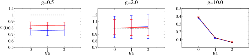
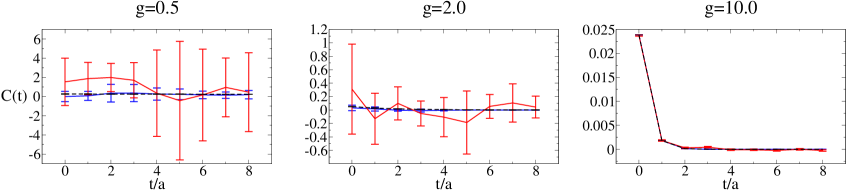
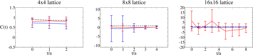
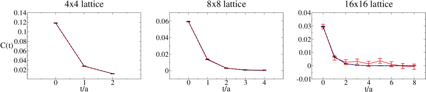
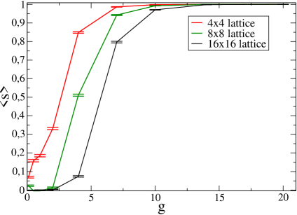
We observe that the correlators are equal within and thus behave as predicted from the analytic results in equation (15). However, for smaller values of the coupling and higher lattice sizes, the large statistical errors due to the sign problem render the results not a significant. The sign problem appears to be more severe in the model as is evident in Fig. 1 and Fig. 3, where we expect that only for very large values of . On the other hand in the case for and for all the lattice volumes that we considered, the expectation value of the sign is approximately 1. The fact that the sign problem improves in theories with a higher number of bosons can be predicted from the form of the matrix in (19): as the term proportional to grows, the spectrum of the matrix becomes more and more positive. To further illustrate the effects of the sign problem on the correlators, we plot the correlators of the and models at a certain value of the coupling in Figure 3. From the plots, it is evident that the effects of the sign problem on the correlators are less visible in the models, even on larger lattice sizes.
The behavior of as a function of the coupling and the lattice volume is shown in Fig. 4. Even though the number of points is limited, we have tried some simple fits of the different with the volume and the coupling. The fit appears consistent with an exponential behavior, decreasing with the volume or the inverse of the coupling [36]. Due to the severe sign problem in the current HMC setting, exploring the range of physical interest, for example, the phase transition at of the model, appears impractical.

6 Outlook
In this work, we have constructed a discretized action and an algorithm for simulating the non-linear sigma model. We have presented numerical results for the bosonic and fermionic two-point functions of the and sigma models.
We have observed the emergence of a sign problem in the simulations. This sign problem comes from admitting negative eigenvalues. For smaller couplings, some eigenvalues appear to fluctuate more and more around zero. The sign problem seems to be milder in the case, with the mean value of the sign approaching for higher values of the coupling. We intend to compute other observables, like the four-point functions and the conserved currents, and to study the behavior of the sign problem in more detail [37].
In future work, we intend to explore algorithms that treat the fermions differently, hoping to ameliorate the sign problem.
7 Acknowledgements
We thank Mika Lauk for sharing his code for the Wolff cluster algorithm. The research of I. C. and J. H. W. is funded by the Deutsche Forschungsgemeinschaft (DFG, German Research Foundation) - Projektnummer 417533893/GRK2575 ”Rethinking Quantum Field Theory”. The research of V.F. is supported by the Heisenberg Professorship program 506208580 “Quantum strings and gauge fields at arbitrary coupling”.
References
- [1] I. Costa, V. Forini, B. Hoare, T. Meier, A. Patella and J.H. Weber, Supersphere non-linear sigma model on the lattice, PoS LATTICE2022 (2023) 367.
- [2] E. Brézin, L. Le Guillou and J. Zinn-Justin, Renormalization of the non-linear -model in (2+) dimension, Phys. Rev. D 14 (1976) .
- [3] A.B. Zamolodchikov, Factorized S-matrices in two dimensions as the exact solutions of certain relativistic quantum field theory models, Annals of Physics 120 (1979) 253.
- [4] V.A. Novikov, M.A. Shifman, A.I. Vainshtein and V.I. Zakharov, Two-Dimensional Sigma Models: Modeling Nonperturbative Effects of Quantum Chromodynamics, Phys. Rept. 116 (1984) 103.
- [5] A. D’Adda, P. Di Vecchia and M. Luscher, Confinement and Chiral Symmetry Breaking in CP**n-1 Models with Quarks, Nucl. Phys. B 152 (1979) 125.
- [6] A.M. Polyakov, Interaction of Goldstone Particles in Two-Dimensions. Applications to Ferromagnets and Massive Yang-Mills Fields, Phys. Lett. B 59 (1975) 79.
- [7] A. Pelissetto and E. Vicari, Critical phenomena and renormalization group theory, Phys. Rept. 368 (2002) 549 [cond-mat/0012164].
- [8] N. Read and H. Saleur, Exact spectra of conformal supersymmetric nonlinear sigma models in two-dimensions, Nucl. Phys. B 613 (2001) 409 [hep-th/0106124].
- [9] H. Saleur and B. Wehefritz-Kaufmann, Integrable quantum field theories with OSP(m / 2n) symmetries, Nucl. Phys. B 628 (2002) 407 [hep-th/0112095].
- [10] H. Saleur and B. Wehefritz Kaufmann, Integrable quantum field theories with supergroup symmetries: The OSP (1/2) case, Nucl. Phys. B 663 (2003) 443 [hep-th/0302144].
- [11] A. Babichenko, Conformal invariance and quantum integrability of sigma models on symmetric superspaces, Phys. Lett. B 648 (2007) 254 [hep-th/0611214].
- [12] V. Mitev, T. Quella and V. Schomerus, Principal Chiral Model on Superspheres, JHEP 11 (2008) 086 [0809.1046].
- [13] A. Cagnazzo, V. Schomerus and V. Tlapak, On the Spectrum of Superspheres, JHEP 03 (2015) 013 [1408.6838].
- [14] M. Alfimov, B. Feigin, B. Hoare and A. Litvinov, Dual description of -deformed OSP sigma models, JHEP 12 (2020) 040 [2010.11927].
- [15] G. Parisi and N. Sourlas, Selfavoiding Walk and Supersymmetry, Journal de Physique Lettres 41 (1980) 403.
- [16] I.A. Gruzberg, A.W.W. Ludwig and N. Read, Exact exponents for the spin quantum Hall transition, Phys. Rev. Lett. 82 (1999) 4524 [cond-mat/9902063].
- [17] T. Quella and V. Schomerus, Superspace conformal field theory, J. Phys. A 46 (2013) 494010 [1307.7724].
- [18] M.R. Zirnbauer, The integer quantum Hall plateau transition is a current algebra after all, Nucl. Phys. B 941 (2019) 458 [1805.12555].
- [19] J.M. Maldacena, The Large N limit of superconformal field theories and supergravity, Adv. Theor. Math. Phys. 2 (1998) 231 [hep-th/9711200].
- [20] R.R. Metsaev and A.A. Tseytlin, Type IIB superstring action in AdS(5) x S**5 background, Nucl. Phys. B 533 (1998) 109 [hep-th/9805028].
- [21] V. Forini, L. Bianchi, M.S. Bianchi, B. Leder and E. Vescovi, Lattice and string worldsheet in AdS/CFT: a numerical study, PoS LATTICE2015 (2016) 244 [1601.04670].
- [22] V. Forini, L. Bianchi, B. Leder, P. Toepfer and E. Vescovi, Strings on the lattice and AdS/CFT, PoS LATTICE2016 (2016) 206 [1702.02005].
- [23] L. Bianchi, M.S. Bianchi, V. Forini, B. Leder and E. Vescovi, Green-Schwarz superstring on the lattice, JHEP 07 (2016) 014 [1605.01726].
- [24] L. Bianchi, V. Forini, B. Leder, P. Töpfer and E. Vescovi, New linearization and reweighting for simulations of string sigma-model on the lattice, JHEP 01 (2020) 174 [1910.06912].
- [25] G. Bliard, I. Costa, V. Forini and A. Patella, Lattice perturbation theory for the null cusp string, Phys. Rev. D 105 (2022) 074507 [2201.04104].
- [26] G. Bliard, I. Costa and V. Forini, Holography on the lattice: the string worldsheet perspective, 2212.03698.
- [27] S. Duane, A.D. Kennedy, B.J. Pendleton and D. Roweth, Hybrid Monte Carlo, Phys. Lett. B 195 (1987) 216.
- [28] M. Hasenbusch, Speeding up the hybrid monte carlo algorithm for dynamical fermions, Physics Letters B 519 (2001) 177.
- [29] A. Hasenfratz, R. Hoffmann and S. Schaefer, Reweighting towards the chiral limit, Phys. Rev. D 78 (2008) 014515.
- [30] M. Luscher and S. Schaefer, Lattice QCD with open boundary conditions and twisted-mass reweighting, Comput. Phys. Commun. 184 (2013) 519 [1206.2809].
- [31] A. Stathopoulos and J.R. McCombs, PRIMME: PReconditioned Iterative MultiMethod Eigensolver: Methods and software description, ACM Transactions on Mathematical Software 37 (2010) 21:1.
- [32] L. Wu, E. Romero and A. Stathopoulos, Primme_svds: A high-performance preconditioned SVD solver for accurate large-scale computations, SIAM Journal on Scientific Computing 39 (2017) S248.
- [33] M. Luscher, Deflation acceleration of lattice QCD simulations, JHEP 12 (2007) 011 [0710.5417].
- [34] R.H. Swendsen and J.-S. Wang, Nonuniversal critical dynamics in monte carlo simulations, Phys. Rev. Lett. 58 (1987) 86.
- [35] U. Wolff, Collective monte carlo updating for spin systems, Phys. Rev. Lett. 62 (1989) 361.
- [36] S. Chandrasekharan and U.-J. Wiese, Meron-cluster solution of fermion sign problems, Phys. Rev. Lett. 83 (1999) 3116.
- [37] I. Costa, V. Forini, B. Hoare, A. Patella and J.H. Weber, in progress, .