Quantum Alternating Operator Ansatz for the Preparation and Detection
of Long-Lived Singlet States in NMR

Abstract

Designing efficient and robust quantum control strategies is vital for developing quantum technologies. One recent strategy is the Quantum Alternating Operator Ansatz (QAOA) sequence that alternatively propagates under two noncommuting Hamiltonians, whose control parameters can be optimized to generate a gate or prepare a state. Here, we describe the design of the QAOA sequence and their variants to prepare long-lived singlet states (LLS) from the thermal state in NMR. With extraordinarily long lifetimes exceeding the spin-lattice relaxation time constant $T_{1}$, LLS have been of great interest for various applications, from spectroscopy to medical imaging. Accordingly, designing sequences for efficiently preparing LLS in a general spin system is crucial. Using numerical analysis, we study the efficiency and robustness of the QAOA sequences over a wide range of errors in the control parameters. Using a two-qubit NMR register, we conduct an experimental study to benchmark QAOA sequences against other prominent methods of LLS preparation and observe the significantly superior performance of the QAOA sequences.

I Introduction

Variational quantum algorithms (VQAs) have emerged as promising candidates for the current noisy intermediate-scale quantum (NISQ) devices and have shown considerable advantage by making optimal use of both quantum resources and classical optimization techniques in what is now popularly known as a hybrid quantum-classical approach [1, 2, 3]. By transforming the optimization problem into a cost function measured on a quantum computer, a classical optimizer varies the parameters of a parametrized quantum circuit to minimize the cost. A particular example of VQAs is the quantum approximate optimization algorithm, initially proposed by Farhi et al. [4] and later generalized to Quantum Alternating Operator Anstaz (QAOA) [5], which employs an alternating sequence of parametrized unitary transformations [6]. Originally designed to solve combinatorial optimization problems such as MaxCut [4, 7, 8, 9], QAOA has found numerous applications in preparing quantum many-body ground states of various ising Hamiltonians [10, 11]. With their remarkable ability to prepare desired quantum states with shallow circuit depths and their utility for universal quantum control [12, 13, 14], QAOA has gained significant attention recently [6]. This paper investigates QAOA for quantum state preparation in nuclear magnetic resonance (NMR) quantum simulators.

In NMR spectroscopy, the spin-lattice relaxation time constant $T_{1}$ determines the rate at which a single spin attains thermal equilibrium from any nonequilibrium state [15]. While an evolving nuclear magnetization captures crucial information about the surrounding physical environment, the $T_{1}$ process gradually restores its thermal equilibrium state, erasing all the information gathered during the dynamics. Therefore, the $T_{1}$ timescale was long believed to be the rigid barrier beyond which no physical process may be studied using nuclear magnetization. In a remarkable discovery two decades ago, Carravetta and Levitt showed the preparation of the singlet order of a nuclear spin pair from thermal magnetization and demonstrated its extraordinarily long lifetime far beyond the $T_{1}$ barrier [16, 17]. Since then, the singlet order in a nearly symmetric spin pair has been popularly known as the Long-Lived State (LLS). The long lifetime of the singlet state is a consequence of its immunity to intra-pair dipole-dipole relaxation, which forms the major source of relaxation in ordinary spin systems. However, it can not connect the antisymmetric singlet state to the symmetric triplet state [18]. In NMR, LLS has been extensively studied [19] and has found numerous applications such as chemical analysis [20], biomedical imaging [21], protein-ligand binding [22, 23, 24], and quantum information processing [25]. More recently, LLS has also been discovered in other architectures [26] and environments [27, 28].

Over the years, several methods for LLS preparation have been developed, which include Carravetta-Levitt (hereafter CL) [17], M2S-S2M [29], SLIC [30], APSOC [31, 32], and optimal control [33, 34]. The CL is a standard method for weakly/moderately coupled spins, whereas M2S-S2M and SLIC are suitable for strongly coupled spins [19]. The above-mentioned methods require precise delays and pulses and work only for weak or strongly coupled systems. On the other hand, adiabatic methods can work for both weak and strongly coupled systems and are robust against experimental imperfections. However, by nature, adiabatic methods require longer times, which may limit their efficiency.

QAOA is a quantum gate-model meta-heuristic that switches between unitaries selected from two types: phase-separation operators and mixing operators [5]. This work demonstrates QAOA as a general method for robust and efficient quantum state preparation by preparing LLS in a pair of nuclear spins (see Fig. 1). We explore three different QAOA sequences and first numerically analyze their performances for spins with different ranges of coupling strengths. We also numerically analyze the inclusion of the counter-diabatic (CD) term in QAOA. We then experimentally demonstrate and benchmark their performances against existing methods, such as APSOC, CL, M2S-S2M, and SLIC.

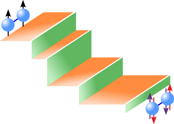
Figure 1: Visualizing the Quantum Alternating Operator Ansatz (QAOA) method for quantum control tasks such as state preparation or gate synthesis.

In Sec. II, we first explain the theoretical framework of QAOA, followed by a formalization of the LLS preparation with/without counter-diabatic term. In section III, we design three types of QAOAs for LLS preparation and perform numerical simulations to analyze their feasibility and robustness in three types of systems: weakly/moderately coupled, strongly coupled, and very strongly coupled. In section IV, we provide an experimental demonstration of all three types of QAOAs in LLS preparation and compare their performances against existing LLS preparation sequences. Finally, we summarize and conclude in section V.

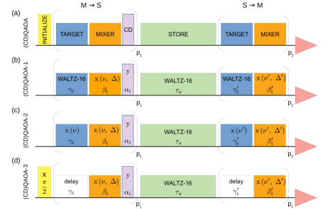
Figure 2: The general (a) and the three particular QAOA sequences (b-d) for LLS preparation, i.e., magnetization to singlet-order transfer (M$\rightarrow$S) and LLS detection, i.e., singlet-order to magnetization transfer (S$\rightarrow$M). Here, $\gamma_{i}^{(}$^′) and $\beta_{i}^{(}$^′) are respectively durations of target and mixer elements, and $\alpha_{i}$ is the duration of optional $I_{y}$ rotation corresponding to CD evolution. The parameters $\nu^{(}$^′) and $\Delta^{(}$^′) are RF pulse strength and RF offset, as described in Table 2. The final observable state in all cases is the single quantum magnetization $I_{1}^{x}I_{2}^{z}-I_{1}^{z}I_{2}^{x}$ that generates a characteristic anti-phase NMR signal [17].

II Theory

II.1 QAOA

As mentioned earlier, QAOA consists of an alternating sequence of two distinct operators. The phase-separation operators $U_{T}(\gamma)=e^{iH_{T}\gamma}$ are parameterized by duration $\gamma$ and are generated by ‘target’ Hamiltonian $H_{T}$, whose eigenstates encode the cost function. The mixing operators $U_{M}(\beta)=e^{iH_{M}\beta}$ are parameterized by duration $\beta$ and generated by a ‘mixer’ Hamiltonian $H_{M}$, which does not commute with $H_{T}$. Therefore, starting from a convenient initial state $\left|{\psi_{I}}\right\rangle$, a QAOA circuit of $p$ layers creates a parameterized state with $2p$ parameters [4]

$$\left|{\psi_{F}}\right\rangle=\left|{\psi(\vec{\gamma},\vec{\beta})}\right\rangle ={U_{Q}}(\vec{\gamma},\vec{\beta})\left|{\psi_{I}}\right\rangle,~{}~{}\mbox{where,}$$

$${U_{Q}}(\vec{\gamma},\vec{\beta}) =\prod_{i=1}^{p}U_{M}(\beta_{i})U_{T}(\gamma_{i}).$$ (1)

To reach the ground state of $H_{T}$, we numerically optimize $\vec{\gamma}$ and $\vec{\beta}$ by minimizing the cost function given by energy $\left\langle{\psi(\vec{\gamma},\vec{\beta})}\right|H_{T}\left|{\psi(\vec{\gamma},\vec{\beta})}\right\rangle$. Alternatively, if we are interested in an arbitrary target state $\left|{\psi_{T}}\right\rangle$, we can numerically optimize $\vec{\gamma}$ and $\vec{\beta}$ by minimizing the infidelity [12]

$$\mathcal{I}_{T}(\vec{\gamma},\vec{\beta})=1-\left|{\left\langle{\psi_{T}}\middle|{\psi(\vec{\gamma},\vec{\beta})}\right\rangle}\right|^{2}.$$ (2)

II.2 Singlet Order Preparation

Consider a pair of two interacting spin-1/2 particles. Starting from a convenient initial state, the goal is to prepare the singlet order, which corresponds to the population difference between the singlet state $\left|{S_{0}}\right\rangle=(\left|{01}\right\rangle-\left|{10}\right\rangle)/\sqrt{2}$ and the equally populated triplet states $\left|{T_{0}}\right\rangle=(\left|{01}\right\rangle+\left|{10}\right\rangle)/\sqrt{2}$, $\left|{T_{+}}\right\rangle=\left|{00}\right\rangle$, and $\left|{T_{-}}\right\rangle=\left|{11}\right\rangle$. In practice, the degenerate triplet eigenstates of isotropic Hamiltonian $-\mathbf{I}_{1}\cdot\mathbf{I}_{2}$ (with spin angular momentum operator $\mathbf{I}$) equilibrate rapidly to equalize their populations spontaneously [17]. For an ensemble system such as an NMR register, if $\rho_{I}$ is the state after initialization, $\rho_{F}={U_{Q}}(\vec{\gamma},\vec{\beta})\rho_{I}{U_{Q}}(\vec{\gamma},\vec{\beta})^{\dagger}$ is the final density matrix and $\rho_{T}$ is the target density matrix, infidelity can be cast as [35]

$$\mathcal{I}_{T}(\vec{\gamma},\vec{\beta})=1-\frac{\mathrm{Tr}(\rho_{F}\rho_{T})}{\sqrt{\mathrm{Tr}(\rho^{2}_{T})Tr(\rho^{2}_{F})}}.$$ (3)

Under the high-temperature approximation in NMR, a density matrix can be written as $\rho=\mathbbm{1}/\mathrm{Tr}[\mathbbm{1}]+\rho_{\Delta}$, where the first term represents the uniform background population that is invariant under the unitary dynamics, and the second term represents the trace-less deviation density matrix that captures all the interesting dynamics [36]. Ignoring the identity term, the thermal state of a two-qubit NMR register is written as $I_{1}^{z}+I_{2}^{z}$, which after initialization by $U_{I}$ becomes $\rho_{I}=U_{I}(I_{1}^{z}+I_{2}^{z})U_{I}^{\dagger}$, and the target state corresponding to the single order is $\rho_{T}=-\mathbf{I}_{1}\cdot\mathbf{I}_{2}$.

Using a $p$-layer QAOA ansatz, we can maximize the singlet content by minimizing the infidelity $\mathcal{I}_{S_{0}}(\vec{\gamma},\vec{\beta})$. In practice, it is also important to simultaneously minimize the total time $\sum_{i=1}^{p}(\gamma_{i}+\beta_{i})$. Therefore, we revise the cost function as

$$f({\vec{\gamma},\vec{\beta}})=r\mathcal{I}_{S_{0}}(\vec{\gamma},\vec{\beta})+(1-r)\sum_{i=1}^{p}(\gamma_{i}+\beta_{i}),$$ (4)

where $r\in[0,1]$ is the positive real weight parameter. For the singlet-order, the infidelity $\mathcal{I}_{S_{0}}$ has a lower bound of $1-\sqrt{2/3}$ [37, 38].

II.3 Counterdiabatic QAOA

Consider an adiabatic control of the form $H(t)=(1-\lambda(t))H_{M}+\lambda(t)H_{T}$, where the scalar parameter $\lambda\in[0,1]$ is driven from 0 to 1 sufficiently slowly to meet adiabaticity [39]. The instantaneous energy gap limits the rate of change of $\lambda$, which often renders the adiabatic control too slow. To overcome this problem, counter diabatic (CD) protocols have been proposed [40, 41], which effectively pull the eigenstates away, widening energy gaps, thereby allowing faster control [42]. Including the first-order CD term $H_{CD}=i\alpha_{1}\dot{\lambda}[H_{M},H_{T}]$ [41], we obtain the control Hamiltonian $H(t)=(1-\lambda(t))H_{M}+\lambda(t)H_{T}+H_{CD}$. While it has been known that QAOA has an inherent counterdiabatic effect [43], the inclusion of $H_{CD}$ further suppresses diabatic transitions. In general, $H_{CD}$ may contain bilinear or other higher-order terms, which may be demanding to implement. It was shown that even an approximate CD term containing only local operators could significantly improve the performance [44]. Thus, for CDQAOA, the net unitary is of the form [43, 45]

$${U_{Q}}(\vec{\gamma},\vec{\beta},\vec{\alpha})=\prod_{i=1}^{p}U_{CD}(\alpha_{i})U_{M}(\beta_{i})U_{T}(\gamma_{i}),$$ (5)

where $U_{CD}({\alpha})=e^{iH_{CD}\alpha}$.

III Numerical analysis of QAOA

Consider a pair of spin qubits with internal NMR Hamiltonian (in a frame rotating at the average Larmor frequency)

$$H_{0}=-\pi\delta(I^{z}_{1}-I^{z}_{2})+2\pi J\mathbf{I}_{1}\cdot\mathbf{I}_{2},$$ (6)

where $\delta$ is the chemical shift difference, $J$ is the scalar coupling constant, and $I^{z}_{i}$ are the z-components of the spin angular momentum operators $\mathbf{I}_{i}$. We numerically analyze the three coupling regimes with specific examples described in Tab. 1.

Table 1: Three types of spin systems are based on the coupling strength to chemical shift ratios, their representative Hamiltonian parameters, and some preferred existing LLS preparation methods. The parameters in the first row belong to the system chosen for experiments.

$\begin{array}[]{c}\mbox{Coupling}\\ \mbox{strength}\end{array}$	$\begin{array}[]{c}\mbox{Representative}\\ \mbox{parameters}\end{array}$		Existing methods
	$\delta$ (Hz)	$J$ (Hz)
Moderate	45.0	17.2	CL, M2S, APSOC
Strong	10.0	18.0	M2S, APSOC, SLIC
Very strong	10.0	54.0	M2S, APSOC, SLIC

It also lists some existing methods for LLS preparation that are preferable for each system type.

We have designed three sequences depending on the type of mixer and target Hamiltonians: QAOA-1, QAOA-2, and QAOA-3, as well as their CD variants. These sequences are pictorially represented in Fig. 2. The explicit forms of the Hamiltonians $H_{M}$ and $H_{T}$ for each sequence and corresponding optimized parameters are listed in Tab. 2.

Table 2: QAOA Hamiltonians and optimized parameters for a moderately coupled system ($\delta=45.0$ Hz, $J=17.2$ Hz). Here $I^{\alpha}=I^{\alpha}_{1}+I^{\alpha}_{2}$ is the total $\alpha$-component of the spin operator. We have chosen the CD term $H_{CD}=I^{y}$ in all the cases. We have used Constrained Optimization By Linear Approximation (COBYLA) implemented in Python’s SciPy [46]. Here, $\tau_{p}$ and $\tau_{d}$ denote the total durations of the preparation and detection sequences, respectively.

Sequence			Preparation				Detection
	$i$	$\nu$	$\Delta$	$\beta_{i}$	$\gamma_{i}$	$\tau_{p}$	$\nu^{\prime}$	$\Delta^{\prime}$	$\beta_{i}^{\prime}$	$\gamma_{i}^{\prime}$	$\tau_{d}$
		(Hz)	(Hz)	(ms)	(ms)	(ms)	(Hz)	(Hz)	(ms)	(ms)	(ms)
QAOA-1
$H_{M}=H_{0}-2\pi\nu I^{x}-2\pi\Delta I^{z}$	1	28.0	20.0	60.936	40.000	101.0	31.0	22.0	50.663	40.000	90.7
$H_{T}=2\pi J\,\mathbf{I_{1}}\cdot\mathbf{I_{2}}$
$\begin{array}[]{c}\textrm{QAOA-2}\\ H_{M}=H_{0}-2\pi\nu I^{x}-2\pi\Delta I^{z}\\ H_{T}=H_{0}-2\pi\nu I^{x}\end{array}$	1	63.0	56.0	1.485	2.227	27.9	77.0	57.0	13.382	1.651	28.9
	2			1.940	0.550				1.710	0.001
	3			9.210	1.663				0.001	1.868
	4			5.518	5.332				7.471	4.398
$\begin{array}[]{c}\textrm{QAOA-3}\\ H_{M}=H_{0}-2\pi\nu I^{x}-2\pi\Delta I^{z}\\ H_{T}=H_{0}\end{array}$	1	200.0	0	0.913	0.386	25.2	200.0	0	2.766	1.839	22.6
	2			1.563	11.234				0.249	0.016
	3			0.001	2.226				0.178	16.207
	4			5.480	3.251				0.444	0.263
	5			0.062	0.111				0.079	0.047
	6								0.465	0.026

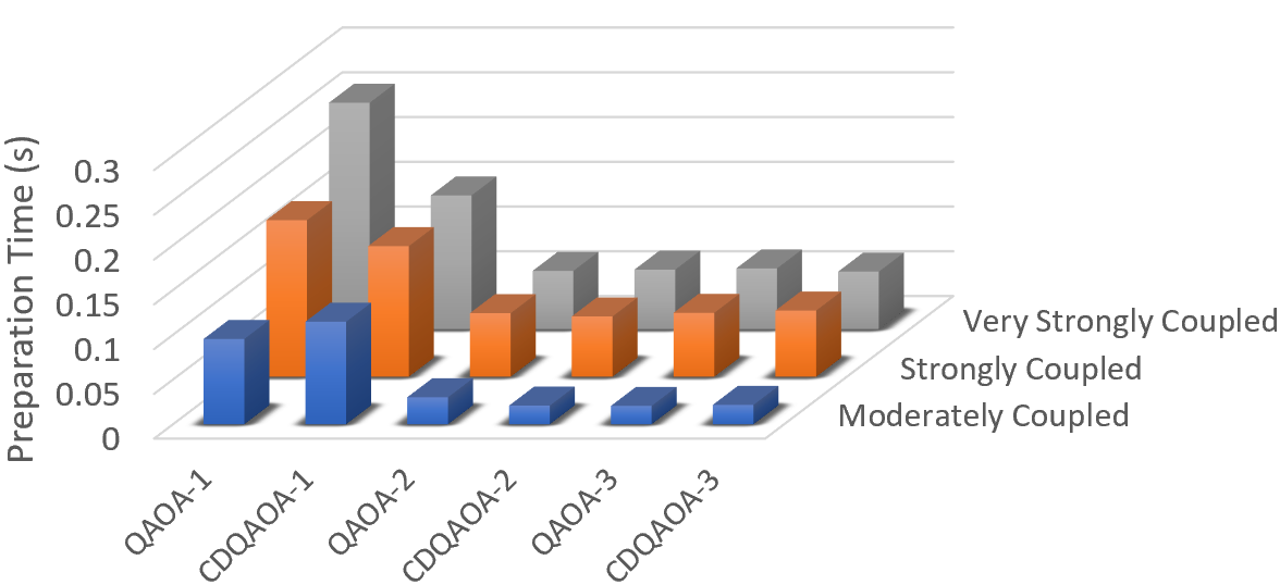
Figure 3: The shortest LLS preparation times for each QAOA sequence sampled from all the sets of control fields that produce a final state fidelity greater than 0.78, about 95% of the theoretical upper bound [37, 38].

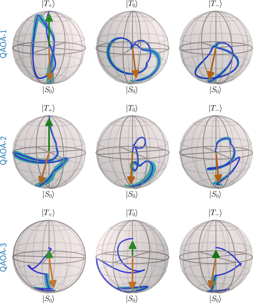
Figure 4: The Bloch sphere trajectory (in $\{\left|{S_{0}}\right\rangle,\left|{T_{0/\pm}}\right\rangle\}$ basis) under each QAOA sequence with parameters in Tab. 2. The dark line corresponds to the nominal control amplitude, and the associated patch corresponds to $\pm 20\%$ deviated control-field amplitude (RF inhomogeneity). The up and down arrows indicate the state after initialization (taken to be $\left|{00}\right\rangle$ for QAOA-1/2 and $\left|{++}\right\rangle$ for QAOA-3) and the final state on the Bloch sphere.

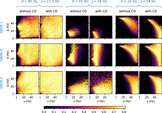
Figure 5: Fidelity heatmaps for 4-layered QAOA sequences obtained by finding the best solution for given $\nu$ and $\Delta$ values.

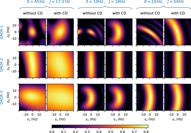
Figure 6: QAOA robustness against deviations $\epsilon_{\Delta}$ and $\epsilon_{\nu}$ (from optimal $\Delta$ and $\nu$ values) introduced during preparation.

Fig. 3 compares the total QAOA duration for preparing LLS with at least a fidelity of 0.78, that is 5% below the upper bound of $\sqrt{2/3}$ [37, 38]. Note that QAOA-2 and QAOA-3 take almost the same durations but are much faster than QAOA-1. Moreover, the isotropic target Hamiltonian $H_{T}=2\pi J\mathbf{I}_{1}\cdot\mathbf{I}_{2}$ in QAOA-1 requires the application of a sophisticated pulse-sequence such as WALTZ-16 and therefore forcing us to put a lower bound on its time discretization [15]. On the other hand, in QAOA-2 and QAOA-3, the target Hamiltonian $H_{T}$ is much simpler to implement: in QAOA-2, $H_{T}$ simply needs a CW pulse, while in QAOA-3 it is just a delay. As one may expect, weakly coupled systems allow much faster LLS preparation in all sequences. To gain an insight into the dynamics under the QAOA sequences, Fig. 4 plots magnetization trajectories in the $\{\left|{S_{0}}\right\rangle,\left|{T_{0/\pm}}\right\rangle\}$ Bloch-spheres. We can notice QAOA-2 and QAOA-3 showing promising approaches to the desired target singlet-order state, despite $\left|{S_{0}}\right\rangle$ not being an eigenstate of their ‘target’ Hamiltonians. QAOA-3 shows the shortest trajectory, although the evolution under $H_{T}=H_{0}$ does not need any external drive and, therefore, it needs minimum resources. This sequence also shows the best experimental performance, as seen in the next section.

The fidelity heatmaps in Fig. 5 show the feasibility ranges of control parameters $\nu$ and $\Delta$ for LLS preparation by QAOA. They indicate that LLS preparation is achievable in a wider range of control parameters in a moderately coupled system compared to a strongly or very strongly coupled system. Interestingly, including the first-order CD term helps slightly expand the favourable range and improve the fidelity of existing regions. From the heatmaps in Fig. 6, we see a marked improvement in the robustness of QAOA sequences against deviations of RF amplitudes $\nu$ and RF offsets $\Delta$ from the optimal values.

IV Experiments

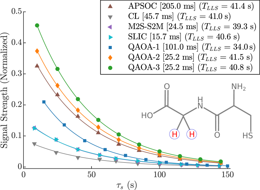
Figure 7: Decay of LLS observed by varying the storage time. All signals are normalized with respect to the signal from thermal magnetization after a $\pi/2$ pulse. The data points are fitted to decaying exponentials, and corresponding $T_{LLS}$ values are mentioned in the legend. The total sequence duration is mentioned within square brackets in each case. The inset shows the molecular structure of Cys-Gly dipeptide, whose two proton spins (circled) form our register.

We now benchmark the performance of the QAOA sequences against standard LLS preparation sequences, namely APSOC [31] and CL [17]. All experiments were done on an 11.7 Tesla Bruker Avance-III NMR spectrometer at an ambient temperature of 300 K. Our system comprises proton spin pairs of Cys-Gly dipeptide (see inset of Fig. 7). The sample was prepared by dissolving 4mg of Cys-Gly in 700 $\mu$L D₂O and bubbled with Argon gas to remove dissolved oxygen. The two nuclear spins are coupled to each other with $J=17.2$ Hz and with the chemical shift difference $\delta=45.0$ Hz (see first row of Tab. 1). We obtained the longitudinal relaxation time constant $T_{1}=1.76$ s from the inversion recovery experiments for both spins. In all experiments, we have used a 1 kHz WALTZ-16 spin-lock sequence to sustain LLS during storage. A two-step phase cycling was used to remove artifacts. All the QAOA Hamiltonians and their optimized experimental parameters are summarized in Tab. 2.

The NMR signal strengths with varying storage times obtained from various preparation methods are shown in Fig. 7. In each case, except QAOA-1, we observe an impressively long decay constant $T_{LLS}$ of about 40 s, about 23 times the $T_{1}$ time-constants of the individual protons. Applying the WALTZ-16 sequence in the detection part of QAOA-1 may have adversely affected its $T_{LLS}$ measurement. The experimental results establish the superiority of QAOA-3 and QAOA-2, despite being shorter than all the sequences except SLIC, whose efficiency is significantly lower. QAOA-3 shows the best performance and is the easiest among all QAOA sequences.

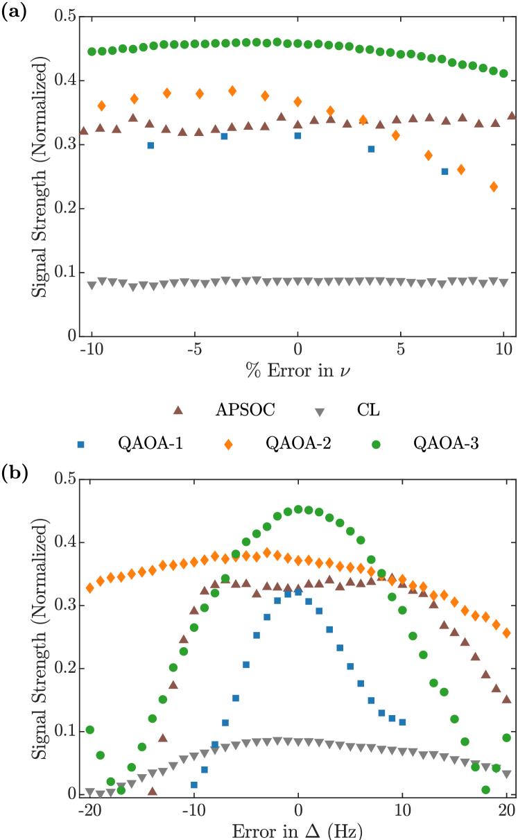
Figure 8: Robustness of the QAOA sequences with respect to (a) RF amplitude $\nu$ and (b) RF frequency offset $\Delta$.

Fig. 8 shows the experimentally obtained robustness of various methods against deviations in the RF amplitudes and offsets. Once again, QAOA-3 shows the best performance against amplitude deviations by as much as $\pm 10\%$, although it is somewhat sensitive to larger offsets beyond $\pm 10$ Hz. On the other hand, QAOA-2 shows better robustness over offset errors up to $\pm 20$ Hz. We notice a general agreement between the experimental robustness plots of Fig. 8 with the simulation robustness plots of Fig. 6. The relative performances of the three QAOA sequences are compared in Tab. 3.

Table 3: Comparison of the performance and the robustness of the three QAOA sequences.

Sequence	Efficiency	RFI	Offset
		robustness	robustness
QAOA-1	$\bigstar$	$\bigstar$	$\bigstar$
QAOA-2	$\bigstar$ $\bigstar$	$\bigstar$ $\bigstar$	$\bigstar$ $\bigstar$ $\bigstar$
QAOA-3	$\bigstar$ $\bigstar$ $\bigstar$	$\bigstar$ $\bigstar$ $\bigstar$	$\bigstar$ $\bigstar$

V Discussions and Conclusions

Robust quantum control is crucial for future quantum technologies, and accordingly, numerous quantum control methods have been developed [47]. The recent QAOA method comprises alternating unitaries generated by two Hamiltonians whose parameters are classically optimized for efficient gate or state synthesis. In some sense, QAOA generalizes over the bang-bang quantum control, which has been demonstrated earlier [48, 49, 50]. Here, we have demonstrated the superior performance of QAOA for state preparation, specifically in preparing the long-lived singlet state (LLS). Since its discovery, LLS has found several applications, from spectroscopy to medical imaging to quantum information.

We have designed three QAOA sequences and experimentally compared their performances against other standard LLS preparation methods, such as CL, APSOC, M2S-S2M, and SLIC. We have made extensive numerical analyses to study the feasibility and robustness of QAOA sequences for different ranges of system parameters and control field parameters. We have also incorporated the counter-diabatic evolution with the help of a third unitary and observed an enhancement in robustness. While there are several methods for LLS preparation in NMR, only a few, such as M2S-S2M, APSOC, and SLIC, work reasonably well for strongly coupled systems. Our numerical studies confirm that QAOA can efficiently prepare LLS across all systems, whether weakly or strongly coupled.

We hope such efficient preparation and detection sequences will advance the scope of LLS applications. We also envisage the applications of QAOA as a general quantum control protocol for various tasks in quantum computing and other fields such as spectroscopy, imaging, etc.

References

- Cerezo et al. [2021] M. Cerezo, A. Arrasmith, R. Babbush, S. C. Benjamin, S. Endo, K. Fujii, J. R. McClean, K. Mitarai, X. Yuan, L. Cincio, et al., Variational quantum algorithms, Nature Reviews Physics 3, 625 (2021).
- Bharti et al. [2022] K. Bharti, A. Cervera-Lierta, T. H. Kyaw, T. Haug, S. Alperin-Lea, A. Anand, M. Degroote, H. Heimonen, J. S. Kottmann, T. Menke, W.-K. Mok, S. Sim, L.-C. Kwek, and A. Aspuru-Guzik, Noisy intermediate-scale quantum algorithms, Rev. Mod. Phys. 94, 015004 (2022).
- McClean et al. [2016] J. R. McClean, J. Romero, R. Babbush, and A. Aspuru-Guzik, The theory of variational hybrid quantum-classical algorithms, New Journal of Physics 18, 023023 (2016).
- Farhi et al. [2014] E. Farhi, J. Goldstone, and S. Gutmann, A quantum approximate optimization algorithm, arXiv preprint arXiv:1411.4028 https://doi.org/10.48550/arXiv.1411.4028 (2014).
- Hadfield et al. [2019] S. Hadfield, Z. Wang, B. O’gorman, E. G. Rieffel, D. Venturelli, and R. Biswas, From the quantum approximate optimization algorithm to a quantum alternating operator ansatz, Algorithms 12, 34 (2019).
- Blekos et al. [2024] K. Blekos, D. Brand, A. Ceschini, C.-H. Chou, R.-H. Li, K. Pandya, and A. Summer, A review on quantum approximate optimization algorithm and its variants, Physics Reports 1068, 1 (2024).
- Zhou et al. [2020] L. Zhou, S.-T. Wang, S. Choi, H. Pichler, and M. D. Lukin, Quantum approximate optimization algorithm: Performance, mechanism, and implementation on near-term devices, Phys. Rev. X 10, 021067 (2020).
- Harrigan et al. [2021] M. P. Harrigan, K. J. Sung, M. Neeley, K. J. Satzinger, F. Arute, K. Arya, J. Atalaya, J. C. Bardin, R. Barends, S. Boixo, et al., Quantum approximate optimization of non-planar graph problems on a planar superconducting processor, Nature Physics 17, 332 (2021).
- Farhi et al. [2022] E. Farhi, J. Goldstone, S. Gutmann, and L. Zhou, The Quantum Approximate Optimization Algorithm and the Sherrington-Kirkpatrick Model at Infinite Size, Quantum 6, 759 (2022).
- Ho and Hsieh [2019] W. W. Ho and T. H. Hsieh, Efficient variational simulation of non-trivial quantum states, SciPost Phys. 6, 029 (2019).
- Pagano et al. [2020] G. Pagano, A. Bapat, P. Becker, K. S. Collins, A. De, P. W. Hess, H. B. Kaplan, A. Kyprianidis, W. L. Tan, C. Baldwin, L. T. Brady, A. Deshpande, F. Liu, S. Jordan, A. V. Gorshkov, and C. Monroe, Quantum approximate optimization of the long-range ising model with a trapped-ion quantum simulator, Proceedings of the National Academy of Sciences 117, 25396 (2020).
- Matos et al. [2021] G. Matos, S. Johri, and Z. Papić, Quantifying the efficiency of state preparation via quantum variational eigensolvers, PRX Quantum 2, 010309 (2021).
- Lloyd [2018] S. Lloyd, Quantum approximate optimization is computationally universal (2018), arXiv:1812.11075 [quant-ph] .
- Morales et al. [2020] M. E. Morales, J. D. Biamonte, and Z. Zimborás, On the universality of the quantum approximate optimization algorithm, Quantum Information Processing 19, 10.1007/s11128-020-02748-9 (2020).
- Cavanagh et al. [2007] J. Cavanagh, W. J. Fairbrother, A. G. Palmer, M. Rance, and N. J. Skelton, Protein NMR Spectroscopy: Principles and Practice, second edition ed. (Academic Press, 2007).
- Carravetta et al. [2004] M. Carravetta, O. G. Johannessen, and M. H. Levitt, Beyond the limit: Singlet nuclear spin states in low magnetic fields, Phys. Rev. Lett. 92, 153003 (2004).
- Carravetta and Levitt [2004] M. Carravetta and M. H. Levitt, Long-lived nuclear spin states in high-field solution nmr, Journal of the American Chemical Society 126, 6228 (2004), pMID: 15149209.
- Pileio [2020a] G. Pileio, ed., Long-lived Nuclear Spin Order, New Developments in NMR (The Royal Society of Chemistry, 2020) pp. P001–441.
- Pileio [2020b] G. Pileio, Long-lived nuclear spin order: theory and applications (Royal Society of Chemistry, 2020).
- Cavadini et al. [2005] S. Cavadini, J. Dittmer, S. Antonijevic, and G. Bodenhausen, Slow diffusion by singlet state nmr spectroscopy, Journal of the American Chemical Society 127, 15744 (2005), pMID: 16277516.
- Glöggler et al. [2017] S. Glöggler, S. J. Elliott, G. Stevanato, R. C. Brown, and M. H. Levitt, Versatile magnetic resonance singlet tags compatible with biological conditions, RSC advances 7, 34574 (2017).
- Salvi et al. [2012] N. Salvi, R. Buratto, A. Bornet, S. Ulzega, I. Rentero Rebollo, A. Angelini, C. Heinis, and G. Bodenhausen, Boosting the sensitivity of ligand-protein screening by nmr of long-lived states, Journal of the American Chemical Society 134, 11076 (2012).
- Buratto et al. [2014] R. Buratto, D. Mammoli, E. Chiarparin, G. Williams, and G. Bodenhausen, Exploring weak ligand-protein interactions by long-lived nmr states: improved contrast in fragment-based drug screening, Angewandte Chemie International Edition 53, 11376 (2014).
- Buratto et al. [2016] R. Buratto, D. Mammoli, E. Canet, and G. Bodenhausen, Ligand–protein affinity studies using long-lived states of fluorine-19 nuclei, Journal of medicinal chemistry 59, 1960 (2016).
- Roy and Mahesh [2010] S. S. Roy and T. S. Mahesh, Initialization of nmr quantum registers using long-lived singlet states, Phys. Rev. A 82, 052302 (2010).
- Chen et al. [2017] Q. Chen, I. Schwarz, and M. B. Plenio, Steady-state preparation of long-lived nuclear spin singlet pairs at room temperature, Phys. Rev. B 95, 224105 (2017).
- Nagashima et al. [2014] K. Nagashima, D. K. Rao, G. Pages, S. S. Velan, and P. W. Kuchel, Long-lived spin state of a tripeptide in stretched hydrogel, Journal of biomolecular NMR 59, 31 (2014).
- Varma and Mahesh [2023] V. Varma and T. S. Mahesh, Long-lived singlet state in an oriented phase and its survival across the phase transition into an isotropic phase, Phys. Rev. Appl. 20, 034030 (2023).
- Pileio et al. [2010] G. Pileio, M. Carravetta, and M. H. Levitt, Storage of nuclear magnetization as long-lived singlet order in low magnetic field, Proceedings of the National Academy of Sciences 107, 17135 (2010).
- DeVience et al. [2013] S. J. DeVience, R. L. Walsworth, and M. S. Rosen, Preparation of nuclear spin singlet states using spin-lock induced crossing, Phys. Rev. Lett. 111, 173002 (2013).
- Pravdivtsev et al. [2016] A. N. Pravdivtsev, A. S. Kiryutin, A. V. Yurkovskaya, H.-M. Vieth, and K. L. Ivanov, Robust conversion of singlet spin order in coupled spin-1/2 pairs by adiabatically ramped rf-fields, Journal of Magnetic Resonance 273, 56 (2016).
- Rodin et al. [2019] B. A. Rodin, K. F. Sheberstov, A. S. Kiryutin, J. T. Hill-Cousins, L. J. Brown, R. C. D. Brown, B. Jamain, H. Zimmermann, R. Z. Sagdeev, A. V. Yurkovskaya, and K. L. Ivanov, Constant-adiabaticity radiofrequency pulses for generating long-lived singlet spin states in nmr, The Journal of Chemical Physics 150, 064201 (2019).
- Wei et al. [2020] D. Wei, J. Xin, K. Hu, and Y. Yao, Preparation of long-lived states in a multi-spin system by using an optimal control method, ChemPhysChem 21, 1326 (2020).
- Khurana and Mahesh [2017] D. Khurana and T. Mahesh, Bang-bang optimal control of large spin systems: Enhancement of 13c–13c singlet-order at natural abundance, Journal of Magnetic Resonance 284, 8 (2017).
- Fortunato et al. [2002] E. M. Fortunato, M. A. Pravia, N. Boulant, G. Teklemariam, T. F. Havel, and D. G. Cory, Design of strongly modulating pulses to implement precise effective Hamiltonians for quantum information processing, The Journal of Chemical Physics 116, 7599 (2002).
- Suter and Mahesh [2008] D. Suter and T. S. Mahesh, Spins as qubits: Quantum information processing by nuclear magnetic resonance, The Journal of Chemical Physics 128, 052206 (2008).
- Singha Roy and Mahesh [2010] S. Singha Roy and T. Mahesh, Density matrix tomography of singlet states, Journal of Magnetic Resonance 206, 127 (2010).
- Pileio [2017] G. Pileio, Singlet nmr methodology in two-spin-1/2 systems, Progress in Nuclear Magnetic Resonance Spectroscopy 98-99, 1 (2017).
- Born and Fock [1928] M. Born and V. Fock, Beweis des adiabatensatzes, Zeitschrift für Physik 51, 165 (1928).
- Kolodrubetz et al. [2017] M. Kolodrubetz, D. Sels, P. Mehta, and A. Polkovnikov, Geometry and non-adiabatic response in quantum and classical systems, Physics Reports 697, 1 (2017).
- Claeys et al. [2019] P. W. Claeys, M. Pandey, D. Sels, and A. Polkovnikov, Floquet-engineering counterdiabatic protocols in quantum many-body systems, Phys. Rev. Lett. 123, 090602 (2019).
- Suresh et al. [2023] A. Suresh, V. Varma, P. Batra, and T. S. Mahesh, Counterdiabatic driving for long-lived singlet state preparation, The Journal of Chemical Physics 159, 024202 (2023).
- Wurtz and Love [2022] J. Wurtz and P. J. Love, Counterdiabaticity and the quantum approximate optimization algorithm, Quantum 6, 635 (2022).
- Sels and Polkovnikov [2017] D. Sels and A. Polkovnikov, Minimizing irreversible losses in quantum systems by local counterdiabatic driving, Proceedings of the National Academy of Sciences 114, E3909 (2017).
- Chai et al. [2022] Y. Chai, Y.-J. Han, Y.-C. Wu, Y. Li, M. Dou, and G.-P. Guo, Shortcuts to the quantum approximate optimization algorithm, Phys. Rev. A 105, 042415 (2022).
- Virtanen et al. [2020] P. Virtanen, R. Gommers, T. E. Oliphant, M. Haberland, T. Reddy, D. Cournapeau, E. Burovski, P. Peterson, W. Weckesser, J. Bright, S. J. van der Walt, M. Brett, J. Wilson, K. J. Millman, N. Mayorov, A. R. J. Nelson, E. Jones, R. Kern, E. Larson, C. J. Carey, İ. Polat, Y. Feng, E. W. Moore, J. VanderPlas, D. Laxalde, J. Perktold, R. Cimrman, I. Henriksen, E. A. Quintero, C. R. Harris, A. M. Archibald, A. H. Ribeiro, F. Pedregosa, P. van Mulbregt, and SciPy 1.0 Contributors, SciPy 1.0: Fundamental Algorithms for Scientific Computing in Python, Nature Methods 17, 261 (2020).
- Mahesh et al. [2023] T. Mahesh, P. Batra, and M. H. Ram, Quantum optimal control: Practical aspects and diverse methods, Journal of the Indian Institute of Science 103, 591 (2023).
- Bhole et al. [2016] G. Bhole, V. S. Anjusha, and T. S. Mahesh, Steering quantum dynamics via bang-bang control: Implementing optimal fixed-point quantum search algorithm, Phys. Rev. A 93, 042339 (2016).
- Yang et al. [2017] Z.-C. Yang, A. Rahmani, A. Shabani, H. Neven, and C. Chamon, Optimizing variational quantum algorithms using pontryagin’s minimum principle, Phys. Rev. X 7, 021027 (2017).
- Liang et al. [2020] D. Liang, L. Li, and S. Leichenauer, Investigating quantum approximate optimization algorithms under bang-bang protocols, Phys. Rev. Res. 2, 033402 (2020).