Root Cause Analysis of Outliers with Missing Structural Knowledge

Abstract

Recent work conceptualized root cause analysis (RCA) of anomalies via quantitative contribution analysis using causal counterfactuals in structural causal models (SCMs). The framework comes with three practical challenges: (1) it requires the causal directed acyclic graph (DAG), together with an SCM, (2) it is statistically ill-posed since it probes regression models in regions of low probability density, (3) it relies on Shapley values which are computationally expensive to find.

In this paper, we propose simplified, efficient methods of root cause analysis when the task is to identify a unique root cause instead of quantitative contribution analysis. Our proposed methods run in linear order of SCM nodes and they require only the causal DAG without counterfactuals. Furthermore, for those use cases where the causal DAG is unknown, we justify the heuristic of identifying root causes as the variables with the highest anomaly score.

1 Introduction

Detecting anomalies in a large number of variables has become a huge effort in science and business application, ranging from meteorology [1], monitoring medical health [2, 3], monitoring of industrial fabrication [4], fraud detection [5], credit scoring [6], cloud applications [7, 8, 9, 10, 11, 12] and more [13, 14, 15, 16, 17]. Oftentimes it is not only important to detect the anomalies but also to answer the question of why the anomaly was observed, or in other words, find its root cause. This is important as it provides insight on how to mitigate the issue manifested in the anomaly, and is hence more actionable. A series of previous works use statistical correlations between features to explain the anomalous value in the target variable [18, 19, 20, 21, 22]. The major drawback with such approaches is that correlations between the anomalous variables and the target variable do not necessarily imply causation. Furthermore, such correlation-based approaches neglect the fact that very small perturbations in some variables can cause extreme anomalies in others. Hence, recent works conceptualized RCA using a causal framework [23, 10, 24, 25, 26]. From a causal perspective, finding causal relations between anomalies that are simultaneously or consecutively observed in different variables is an important step in identifying the root cause, i.e., answering the question of which anomaly caused the other.

Related work We can categorize the related work into two groups: 1) those that require the causal DAG to find the root cause, and, 2) those which do not require the causal DAG or try to infer it from data. Considering the first lines of work, our work builds on [23] in terms of the definition of root cause, where the authors use a causal graphical model based framework and utilize Shapley values to quantify the contribution of each of the variables to the extremeness of the target variable. [27, 28, 9] use a traversal-based approach that identifies a node as a root cause under two conditions: 1) none of its parent nodes exhibits anomalous behavior and 2) it is linked to the anomalous target node through a path of anomalous nodes. [29] apply such a traversal algorithm to data from cloud computing to find the root cause of performance drops in dependent services [12, 30, 31]. The main idea behind the second line of work is that if the DAG is unknown, the outliers themselves can support causal discovery. In a scenario where several data points are available from the anomalous state (which we do not assume here), finding the root cause can also be modeled as the problem of identifying the intervention target of a soft intervention [32]. Likewise, [33, 34] describe how to use heavy-tailed distributions to infer the causal DAG for linear models. In a sense, this also amounts to using outliers for causal discovery – if one counts points in the tail as outliers.

Our contributions This paper tries to mitigate the practical challenges of RCA under the assumption that the task is restricted to identifying a unique root cause whose contribution dominates contributions of the other nodes, rather than quantitative contribution analysis. To this end, we relax the assumptions on the available causal information step by step: In Section 3, we first explain that interventional probabilities are sufficient and we do not need to rely on structural equation based counterfactuals. This finding enables us to design the Topologically Ordered Contribution Analysis (TOCA) algorithm. In Section 4 we discuss how to avoid the statistical problem of estimating interventional probabilities and propose SMOOTH TRAVERSAL, an algorithm that inputs only the causal graph, and SCORE ORDERING, an algorithm that is only based on the ordering of the anomaly scores and hence, does not even need the causal graph. All our methods avoid a combinatorial explosion of terms in Shapley value based RCA. Section 5 compares the approaches on simulated and real-world data.

2 Formal Framework for Root Cause Analysis

We first sketch the causal framework that our method and analysis are based on [36, 35]. Consider a system of $n$ random variables $(X_{1},\dots,X_{n}):=\mathbf{X}$ and an underlying DAG corresponding to the causal relations between them in a way that a directed edge from $X_{i}$ to $X_{j}$ indicates that $X_{i}$ directly causes $X_{j}$. Furthermore, we are given an SCM with structural equations

$$X_{i}:=f_{i}(Pa_{i},N_{i}),$$ (1)

which indicates that each variable $X_{i}$ is a function of its parents ${Pa}_{i}$ together with a noise variable $N_{i}$, where $(N_{1},\ldots,N_{n}):=\mathbf{N}$ are jointly independent. We always assume $X_{n}$ to be the sink note and the target of interest, whose anomaly is supposed to be explained via root causes further upstream. An iterative use of Eq. 1 results in a representation

$$X_{n}=F(N_{1},\dots,N_{n}),$$ (2)

in which the structural causal information is implicit in the function $F$.

Consider the case where the value $x_{n}$ of the target variable $X_{n}$ is flagged as an outlier, and we wish to find the unique root cause of this outlier among the variables $(X_{1},\ldots,X_{n})$. By Eq. 2 we have that

$$x_{n}=F(n_{1},\dots,n_{n}),$$

where $(n_{1},\dots,n_{n}):=\mathbf{n}$ denote the corresponding values of the noise variables. This representation allows us to consider the contribution of each variable $X_{i}$ to the outlier value in $x_{n}$ in the target variable as the contribution of its noise term [23, 38]. The idea of attributing anomalies to noise terms is justified by the perspective that each $n_{j}$ switches between deterministic mechanisms $f_{j}(.,n_{j})$, “response functions” [39], and the goal of RCA is to identify the “corrupted mechanisms” which did not work as usual, i.e., the values $x_{j}$ that do not follow the SCM $x_{j}=f_{j}(pa_{j},n_{j})$ with a value $n_{j}$ “in a normal range”. In other words, the recursive formulation allows us to attribute the extremeness in $x_{n}$ to a corrupted noise term at one of the upstream nodes. As a result, the framework is based on the intuition that if $X_{j}$ is the unique root cause, then replacing $n_{j}$ with a normal value would change $x_{n}$ to a non-outlier, with high probability.

2.1 Anomaly Score

We next define an outlier score which we use in the next sections for our method and analysis. Let $g:\mathcal{X}\rightarrow\mathbb{R}$ be an appropriate feature map. This feature map can be any existing outlier score function mapping elements of $\mathcal{X}$ to real values, for example, z-score. Further, define the event

$$E:=\{g(X_{n})\geq g(x_{n})\},$$ (3)

of being more extreme than the observed event $x_{n}$ according to the feature function $g$. From the point of view of statistical testing, $g$ can be seen as test statistics for the null hypothesis that $x_{n}$ is drawn from $P(X_{n})$, i.e., $H_{0}:x_{n}\sim P(X_{n})$, and $P(g(X_{n})\geq g(x_{n}))=P(E)$ is the corresponding p-value. Note that small $P(E)$ indicates that the null hypothesis is rejected with high confidence and we rather assume that the usual mechanism generating samples from $P(X_{n})$ has been corrupted for that specific statistical unit. Since small p-values correspond to strong anomalies, we define the anomaly score by

$$S(x_{n})=-\log P(g(X_{n})\geq g(x_{n}))=-\log P(E).$$ (4)

Since the logarithm of the probability of an event measures its ‘surprise’ in information theory  [13, 15], as in [23], we call anomaly scores with the above calibration ‘IT scores’ for information theoretic. Given $k$ observations $x_{n}^{1},\dots,x^{k}_{n}$ from $P(X_{n})$, we will often use the following simple estimator

$$\hat{S}(x_{n}^{k}):=-\log\frac{1}{k}|\{i\leq k\,|\,\,\hbox{with }g(x^{i}_{n})\geq g(x^{k}_{n})\}|.$$ (5)

It is important to note that this value can be at most $\log k$. As a result, for the estimate $\hat{S}(x_{n})$, at least $e^{\hat{S}(x_{n})}$ data samples must have been used.

2.2 Contribution Analysis

To compute the contribution of each noise $N_{i}$ to the anomaly score of the outlier $x_{n}$, [23] measure how replacing the observed value $n_{i}$ (originating from a potentially corrupted mechanism) with a normal value, changes the likelihood of the outlier event. Intuitively, this shows us the extent to which $n_{i}$ has been responsible for the extremeness of $x_{n}$. This change of probability, however, should be measured given different contexts, with each context being the set of variables that are already changed to a normal value. To formalize this, for any subset of the index set, ${\mathcal{S}}\subseteq\mathcal{U}:=\left\{1,\ldots,n\right\}$, we first define the probability of the outlier event when all nodes in $\bar{{\mathcal{S}}}=\mathcal{U}\setminus{\mathcal{S}}$ are randomized according to their joint distribution, and only those in ${\mathcal{S}}$ are kept fixed, i.e.,

$$q({\mathcal{S}}):=P(E\,|\,{\bf N}_{{\mathcal{S}}}={\bf n}_{{\mathcal{S}}}).$$ (6)

Now the contribution of a node $j$ given the context $\bar{{\mathcal{S}}}$ is defined as:

$$C(j|\bar{{\mathcal{S}}}):=\log\frac{q({\mathcal{S}}\cup\{j\})}{q({\mathcal{S}})}.$$ (7)

Let $\Pi:\mathcal{U}\rightarrow\mathcal{U}$ be the set of all possible permutations of the nodes and $\pi\in\Pi$ be any permutation. One then defines the contribution of a node $j$ given permutation $\pi$ as

$$C^{\pi}(j):=C(j|I^{\pi>j}),$$ (8)

where $I^{\pi>j}$ denotes the set of nodes that appear after $j$ with respect to $\pi$, i.e., $I^{\pi<j}=\left\{i\in\mathcal{U}\,|\,\pi_{i}<\pi_{j}\right\}$. One can easily see that for each permutation $\pi$, $S(x_{n})$ decomposes into the contributions of each node:

$$S(x_{n})=\sum_{j\in\left\{1,\ldots,n\right\}}C^{\pi}(j).$$

To symmetrize over all the possible permutations in $\Pi$, the Shapley contribution is calculated as:

$$C^{Sh}(j):=\frac{1}{n!}\sum_{\pi\in\Pi}C(j|I^{\pi>j}),$$ (9)

which is certainly expensive to compute [23]. Here, however, motivated by the fact that in most real-world scenarios there is a single corrupted factor causing anomalies, we try to find the unique node $j$ with a corrupted mechanism, or the unique root cause of the outlier $x_{n}$. As our first result, we show that in this scenario, it is unlikely that nodes other than $j$ get a significant value for their contribution. Note that this directly allows us to identify the root cause without the need for quantitatively finding the contribution of each and every node in the outlier value of the target variable $X_{n}$, which saves us exponential computations. In addition to the computational load, the symmetrization suffers from a more fundamental issue, namely that for most permutations $\pi$, the contributions $C^{\pi}(j)$ rely on structural equations (rung 3 causal information according to the ladder of causation in [35]), while some $C^{\pi}(.)$ rely only on the graphical model (rung 2), which we explain in the next sub-section.

2.3 Interventional vs Counterfactual RCA

Since the SCM cannot be inferred from observational and interventional data, relying on the SCM is a serious bottleneck for RCA. Fortunately, no term in Eq. 9 requires the SCM. We explain this through an example for the bivariate causal relation $X_{1}\to X_{2}$: given the SCM $X_{2}=f(X_{1},N_{2}$) and $X_{1}=N_{1}$, randomizing $N_{2}$ and fixing $N_{1}=n_{1}=x_{1}$ generates $X_{2}$ according to the observational conditional $P(X_{2}|x_{1})$ (which no longer relies on the SCM), while, randomizing $N_{1}$ and adjusting $N_{2}=n_{2}$ cannot be resolved into any observational term (see also Section 5 in [41]). The following result generalizes this insight:

Proposition 2.1

Whenever $\pi$ is a topological order of the causal DAG, i.e., there are no arrows $X_{i}\to X_{j}$ for $\pi(i)>\pi(j)$, all contributions $C^{\pi}(j)$ can be computed from observational conditional distributions.

All proofs can be found in Appendix A. While [23] introduced Shapley contribution in Eq. 9 for a quantitative contribution analysis, we are interested in finding the unique root cause whenever it exists. In other words, we are not interested in ‘fair’ quantitative attribution analysis since we assume that one node is dominating anyway, regardless of which order we choose.

3 Simplified contribution analysis without counterfactuals

While we can never exclude the case where several mechanisms are corrupted, we always start with the working hypothesis that there has been only one. If this does not work, we can still try out hypotheses with more than one, but with the strong inductive bias of preferring explanations where most mechanisms worked as expected, in agreement with the so-called ‘sparse mechanism shift hypothesis’ in [42, 43].

To formalize the assumption of a unique root cause, we first generalize the notion of the contribution of a node to the contribution of a set $\mathcal{R}\subseteq\mathcal{U}$ of nodes given a context $\bar{{\mathcal{S}}}$, i.e.,

$$C(\mathcal{R}|\bar{{\mathcal{S}}}):=\log\frac{q({\mathcal{S}}\cup\mathcal{R})}{q({\mathcal{S}})}.$$ (10)

This notion becomes rather intuitive after observing that it is given by the sum of the contributions of all the elements in $\mathcal{R}$ when they are one by one added to the context $\bar{{\mathcal{S}}}$:

Lemma 3.1

For any set $\mathcal{R}\subseteq{\mathcal{T}}\setminus{\mathcal{S}}$, it holds that $C(\mathcal{R}|\bar{{\mathcal{S}}}):=\sum_{i=1}^{k}C(j_{i}|\overline{{\mathcal{S}}\cup\mathcal{R}\setminus\left\{j_{1},\dots,j_{i}\right\}})$ with $\mathcal{R}=\left\{j_{1},\ldots,j_{k}\right\}$.

Next, the following result shows that it is unlikely to obtain high contributions when the noise values are randomly drawn from their usual distributions, i.e., we have the following proposition:

Proposition 3.2

For any set of observed noise values ${\bf n}_{S}$ it holds that $P\left(C(\mathcal{R}|\bar{{\mathcal{S}}})\geq\alpha\right)\leq e^{-\alpha}$.

The way Proposition 3.2 is phrased, it assumes that all noise variables $N_{1},\dots,N_{n}$ follow their usual distributions $P(N_{j})$. This is actually not the case we are interested in. When we observe an anomaly $S(x_{n})$ we assume that at least one mechanism is corrupted for the observation of interest and thus at least for one $j$, the value $n_{j}$ has been drawn from a different distribution $\tilde{P}(N_{j})$. However, one can easily see that the proposition still holds when all $N_{j}$ not in $\mathcal{R}$ are drawn from a different distribution. We therefore read Proposition 3.2 as saying that it is unlikely that non-corrupted nodes have high contributions.

To find the root cause $j$, we will describe an algorithm that replaces step by step each $n_{i}$ with random values $\tilde{n}_{i}$ and estimate how this affects the probability of the event $E$ as in Eq. 3, which we call the outlier event, for short. We observe that for any set ${\mathcal{S}}$, the probability of obtaining an outlier when all noise values in ${\mathcal{S}}$ are randomized can be rewritten in terms of contributions of sets:

Lemma 3.3 (outlier probabilities from contributions of sets)

The probability for the outlier event $E$ when all noise variables in ${\mathcal{S}}$ are randomized can be written in terms of contributions of ${\mathcal{S}}$ or $\bar{{\mathcal{S}}}$, i.e.,

$$C(\bar{\mathcal{S}}\,|\,{\mathcal{S}})\overset{i}{=}e^{C(\bar{{\mathcal{S}}}|{\mathcal{S}})-S(x_{n})}\overset{ii}{=}e^{-C(S|\bar{S})}.$$ (11)

We now consider contributions with respect to a given permutation, $\pi$, of the index set $\mathcal{U}=\left\{1,\ldots,n\right\}$. To this end, remember from the previous section that $I^{\pi<j}$ denotes the set of nodes which appear before $j$ with respect to the permutation $\pi$, i.e., $I^{\pi<j}=\left\{i\in\mathcal{U}\,|\,\pi_{i}<\pi_{j}\right\}$ and likewise for superscripts $\pi>j$, $\pi\geq j$, etc. We first define the dominating root cause with respect to a permutation $\pi\in\Pi$.

Definition 3.4 (dominating root cause with respect to $\pi$)

Node $j$ is said to be the dominating root cause with respect to the permutation $\pi$ if we have for all $i\in I^{\pi\leq j}$

$$(i)\quad C(I^{\pi<i}|I^{\pi\geq i})<S(x_{n})/4,$$

and further, for all $i\in I^{\pi\geq j}$, we have

$$(ii)\quad C(I^{\pi>i}|I^{\pi\leq i})<S(x_{n})/4.$$

The definition is motivated by the assumption that sets that do not contain $j$ have no significant contribution. However, demanding that this holds for all subsets would be far too strong since Proposition 3.2 cannot hold uniformly over all of them. Therefore we only demand it for two dedicated subsets ($I^{\pi<i}$ and $I^{\pi>i}$) which are sufficient for our analysis.

First we observe that for all $i\in I^{\pi<j}$, together with Lemma 3.3, condition (i) of Def. 3.4 implies

$$P(E|{\bf n}_{I^{\pi<i}})\leq e^{-\frac{3}{4}S(x_{n})}.$$ (12)

Further, for all $i\in I^{\pi>j}$ Lemma 3.3 and condition (ii) of Def. 3.4 imply

$$P(E|{\bf n}_{I^{\pi<i}})\geq e^{-\frac{1}{4}S(x_{n})}.$$ (13)

In other words, if we increase the set of nodes for which the actual noise values are replaced with random values node by node, starting from the last one in the ordering $\pi$, then $-\log P(E|{\bf n}_{I^{\pi<i}})$ jumps by at least $S(x_{n})/2$ when we reach the root cause $i=j$. On the other hand, jumps of log probabilities are smaller than $S(x_{n})/2$ at every other node. To tell which of the bounds Eq. 13 and Eq. 12, are valid we need to estimate the probabilities up to an error of

$$\frac{1}{2}(e^{-\frac{1}{4}S(x_{n})}-e^{-\frac{3}{4}S(x_{n})})\geq\frac{1}{4}e^{-\frac{1}{4}S(x_{n})}:=\delta.$$ (14)

The inequality assumes $e^{-S(x_{n})/2}\leq 1/2$, otherwise $x_{n}$ should not be considered an outlier. Next we investigate how many samples we need to use to estimate the probabilities $P(E\,|\,{\bf n}_{I^{\pi<i}})$ up to error level $\delta$:

Lemma 3.5 (Hoeffding bound)

To have $P\left(|\hat{P}(E\,|\,{\bf n}_{I^{\pi<i}})-P(E\,|\,{\bf n}_{I^{\pi<i}})|<\delta~{}\forall i\leq n\right)>1-\alpha$ we need to use at least $k=\frac{\log\frac{2n}{\alpha}}{2\delta^{2}}$ number of data samples.

As an example, for $\alpha=0.1$ and using $n=50$ nodes, we would need $\approx 80e^{S(x_{n})/2}$ number of data sample. If $S(x_{n})$ has been estimated via Eq. 5, it is based on at least $e^{S(x_{n})}$ samples.

For practical applications, we propose Algorithm 1 (TOCA, Topologically Ordered Contribution Analysis) which simply infers the node $i$ for which the estimated log probabilities show the largest jump as the root cause. In what comes next, we discuss different properties of TOCA.

Conceptual difference to traversal algorithm: When we have identified a node $j$ for which the log probabilities of $E$ jump when including $j$ in the conditioning set, we can be certain that $j$ is a root cause in the sense of having high contribution. This is not the case for the traversal algorithm (as used by [27, 28, 9]), which infers the most upstream anomaly as root cause: Let, for instance,

$$X_{1} =N_{1},$$

$$X_{2} =0.1\cdot X_{1}+N_{2},$$

where $X$ and $N_{2}$ are standard Gaussians ${\cal N}(0,1)$. When $x_{1}=-3$ and $n_{2}=3$, traversal identifies $x_{1}$ as the root cause (because both values $x_{1}$ and $x_{2}$ are anomalous), although a more typical value of $X_{1}$ would have made the target outlier $x_{2}$ even stronger. Hence, $x_{1}$ has even a negative contribution in the above sense.

Why do we measure gaps of log probabilities? From the perspective of statistical estimation, it would certainly be easier to seek for the index with the largest increase of probability instead of the largest increase of logarithmic probability of $E$. Why don’t we work with a definition of contribution that is defined by additive increase rather than multiplicative increase? The following example shows that high multiplicative increase can only be caused by rare events, while high additive increase can happen quite frequently: Consider the boolean causal relation between 3 binaries $E=N_{1}\wedge N_{2}$ with $P(N_{1}=1)=1/2$ while $P(N_{2}=1)=0.001$. Then we have $P(E=1|N_{2}=1)=1/2$, while $P(E=1|N_{1}=1,N_{2}=1)=1$. Hence, $n_{1}=1$ increases the probability of $E$ by $1/2$, although this value occurs quite frequently. In contrast, a large multiplicative increase is only achieved by the rare event $n_{2}=1$ (in agreement with Proposition 3.2). The conclusion that large contribution comes from a corrupted mechanism (‘the root cause’) is only justified because high contributions are unlikely otherwise.

Why do we choose a topological order? So far, we have not made use of the fact that $\pi$ is a topological ordering of the causal DAG. We now employ Proposition 2.1 and note that we can replace all our probabilities with observational probabilities:

$$P(E|{\bf n}_{I^{\pi\leq i}})=P(E|{\bf x}_{I^{\pi\leq i}}).$$ (15)

In practice, the easiest way to sample from the conditional distribution $P(E|{\bf x}_{I^{\pi\geq i}})$ would still be to just sample the noise values. This may come as a surprise given that we have advertised not relying on the structural equation as an advantage of the topological ordering. However, the crucial point is that we have nevertheless circumvented the problem of SCMs being ambiguous: We can choose any SCM that generates the observed conditional distribution, regardless of whether it properly describes the counterfactuals. This is because the obtained contributions only depend on the observational conditional probabilities due to Eq. 15.

1:  Input: outlier $x_{n}$, the FCM between the variables $X_{1},\ldots,X_{n}$, a topological ordering of nodes $\pi$

2:  Initialize: $\mathcal{A}=\left\{0\right\}_{i=1}^{n}$

3:  for $\text{itr}\in\left\{1,\ldots,k\right\}$ do

4:     $\tilde{\bf n}=(n^{\prime}_{1},\ldots,n^{\prime}_{n})$

5:     ${\mathcal{S}}=\emptyset$

6:     for $i\in\text{Reverse order of }\pi$ do

7:        ${\mathcal{S}}\rightarrow{\mathcal{S}}\cup\left\{i\right\}$

8:        $\mathcal{A}_{i}\leftarrow\mathcal{A}_{i}+\mathbb{I}[g(F(\tilde{\bf n}_{{\mathcal{S}}}))\geq g(x_{n})]$

9:     end for

10:  end for

11:  return $\mathop{\mathrm{argmax}}_{i\in\left\{1,\ldots,n\right\}}\log\frac{\mathcal{A}_{i-1}}{\mathcal{A}_{i}}$

Algorithm 1 (TOCA) Returns the unique root cause of the outlier $x_{n}$, as define by Def. 3.4.

4 Causal relations between outliers via calibrated anomaly scores

We have discussed methods that do not require SCMs and require only the graphical model, that is, the causal DAG endowed with observational conditional probabilities $P(X_{j}|Pa_{j})$. However, inferring the latter is statistically ill-posed, particularly when the number of parents is large. While the additive noise assumption reduces the problem essentially to the regression problem of estimating conditional expectations, the problem remains ill-posed because analyzing outliers amounts to probing the regression models in regions with low density. Here we describe approaches that infer causal relations between anomalies from a given causal DAG together with marginal anomaly scores $S(x_{j})$, using the simple estimator Eq. 5. To this end, we start with the toy example of cause-effect pairs and then generalize it to more than two variables.

4.1 Outliers of cause-effect pairs

Let the causal DAG be $X\to Y$ for two variables $X,Y$, where we observe anomalies with anomaly scores $S(x),S(y)$ that occur together. We argue now that, the anomaly $x$ is implausible to be the unique root cause of the anomaly $y$ if $S(x)\ll S(y)$. This can be proven subject to the following assumptions:

1. Monotonicity: increasing the anomaly score of $X$ does not decrease the probability of an anomaly event at $Y$:

   $$P\left\{S(Y)\geq S(y)|S(X)=S(x)\right\}\leq P\left\{S(Y)\geq S(y)|S(X)\geq S(x)\right\},$$ (16)

2. Injectivity: the mapping $x\mapsto S(x)$ is one-to-one. This is the case, for instance, for scores obtained from one-sided tail probabilities, that is for $g(x):=x$.

We then define two different null hypotheses stating that the mechanisms $P(X)$ or $P(Y|X)$, respectively, worked as usual: $H^{X}_{0}$: $x$ has been drawn from $P(X)$, and $H^{Y}_{0}$: $y$ has been drawn from $P(Y|X=x)$ (where $P(X,Y)$ denotes the joint distribution of $X,Y$ in the normal mode). Note that $H^{Y}_{0}$ allows that $X$ is drawn from an arbitrary distribution instead of $P(X)$, only the mechanism generating $y$ from $x$ has remained the same. We then have the following criteria for rejecting $H_{0}^{X}$ and $H_{0}^{Y}$:

Lemma 4.1 (rejecting $H^{X}_{0}$)

$H^{X}_{0}$ can be rejected at level $p\leq e^{-S(x)}$.

This follows immediately from the definition of IT scores in Eq. 4. On the other hand, we obtain:

Lemma 4.2 (rejecting $H_{0}^{Y}$)

Subject to Monotonicity and Injectivity assumptions, $H^{Y}_{0}$ can be rejected at level $p\leq e^{-(S(y)-S(x))}$.

Lemma 4.1 and Lemma 4.2 entail interesting consequences for the case where the causal direction is not known: Let $S(x)=10,S(y)=5$. For $X\to Y$ we can only reject $H_{0}^{X}$, while mechanism $P(Y|X)$ possibly worked as expected. However, for $Y\to X$, we would reject both hypotheses, that $P(Y)$ and that $P(X|Y)$ worked as expected with p-level $e^{-5}$ each. Following the working hypothesis that at most one mechanism was corrupted we thus prefer $X\to Y$.

Small sample version When the anomaly scores are estimated from a small number of observations according to Eq.5, comparison of scores can still be insightful: if $\hat{S}(y)\gg\hat{S}(x)$, then for a large fraction of observations $(\tilde{x},\tilde{y})$ for which $g(\tilde{x})\geq g(x)$ the statement $g(\tilde{y})\geq g(y)$ does not hold. Hence, the event $g(\tilde{x})\geq g(x)$ is not a sufficient cause [44] for the event $g(\tilde{y})\geq g(y)$. In this sense, we can still exclude the value with a smaller score as a candidate for the root cause, if we are interested in sufficient causes.

4.2 Outliers in DAGs with multiple nodes

To infer which node in a DAG with $n$ nodes has been corrupted, we start with the hypothesis that all nodes except $j$ worked as expected: $H^{j}_{0}$: for the anomaly event $(x_{1},\dots,x_{n})$ all $x_{i}$ with $i\neq j$ have been drawn from $P(X_{i}|Pa_{i}=pa_{i})$. To define a test statistics, we first introduce the conditional outlier scores from [45]:

$$S(x_{i}|pa_{i}):=-\log P(g(X_{i})\geq g(x_{i})|Pa_{i}=pa_{i}),$$

where $g$ is some feature function as before (we actually allow variable-dependent feature functions $g_{i}$, but they need to coincide between conditional and unconditional outlier scores). With variable input $x_{i},pa_{i}$, they define random variables $S(X_{i}|Pa_{i})$. Further, we add the following assumption to Monotonicity and Injectivity from Subsection 4.1:

• Continuity: all variables $X_{i}$ are continuous with density w.r.t. the Lebesgue measure, and also all conditional distributions $P(X_{i}|Pa_{i}=pa_{i})$ have such a density.

This condition ensures that all the conditional outlier scores are distributed according to the density $p(s)=e^{-s}$, because then the cumulative distribution function is uniformly distributed. It entails a property that will be convenient for testing $H^{j}_{0}$:

Lemma 4.3 (independence of conditional outlier scores)

Subject to the continuity assumption,
$\left\{S(X_{1}|Pa_{1}),\cdots,S(X_{n}|Pa_{n})\right\}$ are independent random variables.

Independence of conditional scores enables the definition of a simple test statistics that is obtained by summing over the individual ones together with a correction term. With the cumulative score: $S_{cum}:=\sum_{i\neq j}S(X_{i}|Pa_{i})$, we have that:

$$S:=S_{cum}-\log\sum_{l=0}^{n-2}\frac{S_{cum}^{l}}{l!}.$$ (17)

To understand Eq.17, note that the second term is needed to ‘recalibrate’ since the sum of independent IT scores is no longer an IT score, but with the extra term, it is. Intuitively, one may think of the extra term as a multi-hypothesis testing correction: the sum of independent IT scores is likely to be large because it is not unlikely that the set contains one large term. The following result states that this is quantitatively the right correction:

Lemma 4.4 (distribution of cumulated score)

If $H^{j}_{0}$ holds, Eq. 17 is distributed according to the density $p(s)=e^{-s}$.

As a direct result of the above lemmas we have:

Theorem 4.5 (p value for $H^{j}_{0}$ from conditional outlier scores)

$H_{0}$ can be rejected for the observation $(x_{1},\dots,x_{n})$ with p-value

$$p=e^{-S_{cum}}\cdot\sum_{l=1}^{n-2}\frac{S_{cum}^{l}}{l!}.$$

The theorem justifies choosing the index $j$ with the maximal conditional outlier score as the root cause, whenever we follow the working hypothesis that only one mechanism is corrupted.

We started this subsection with the goal of avoiding the estimation of conditional probabilities. Therefore, we will now replace conditional outlier scores with bounds derived from marginal anomaly scores, following the ideas from the bivariate case. To this end, we replace the monotonicity assumption from there with two stronger ones. We introduce the ‘outlier events’ $E_{i}:=\{g(X_{i})\geq g(x_{i})\}$ and postulate:

• Monotonicity:

  $$P\{E_{n}|g(Pa_{i})=g(pa_{i})\}\leq P\{E_{n}|g(Pa^{1}_{i})\geq g(pa^{1}_{i}),\dots,g(Pa^{k}_{i})\geq g(pa^{k}_{i})\},$$

• Non-negative dependence: For any $k$ nodes $\left\{i_{1},\dots,i_{k}\right\}$:

  $$P(E_{i_{1}},\dots,E_{i_{k}})\geq P(E_{i_{1}})\cdots P(E_{i_{k}}),$$

where $Pa^{1}_{i},\dots,Pa^{k}_{i}$ denote the parents of $X_{i}$. Both conditions are close in spirit because they assume mutual positive influence of outlier events. While 1a is explicitly causal, 1b is actually a purely statistical condition, but also justified by an implicit causal model in which outliers at one point of the system render outliers at other points more likely and not less. We then obtain the following bound on the joint statistics $S_{cum}$:

Theorem 4.6 (p value from increment of scores)

With the cumulative anomaly score increments: $\hat{S}_{cum}=-\sum_{i\neq j}\left|S(x_{i})-\sum_{l}S(pa^{l}_{i})\right|_{+}$, it holds that if conditions 1a and 1b hold, $H^{j}_{0}$ can be rejected with

$$p\leq e^{-\hat{S}_{cum}}\cdot\sum_{l=1}^{n-2}\frac{\hat{S}_{cum}^{l}}{l!}.$$

4.3 Finding root causes by minimizing score differences

Theorem 4.6 has interesting consequences for the scenario where $n$ variables form the causal chain

$$X_{1}\to X_{2}\cdots\to X_{n}.$$ (18)

In this case, $\hat{S}_{\text{cum}}$ reduces to the sum of score differences for adjacent nodes. Accordingly, $H^{j}_{0}$ can then be rejected at p-value:

$$p\leq\left\{\begin{array}[]{c}e^{-S(x_{1})-\sum_{i\neq j,i\geq 2}|S(x_{i})-S(x_{i-1})|_{+}}\hbox{ for }i\neq 1\\ e^{-\sum_{i\geq 2}|S(x_{i})-S(x_{i-1})|_{+}}\hbox{ for }i=1\end{array}\right.$$ (19)

We conclude that $H^{j}_{0}$ needs to be rejected whenever the anomaly score increases significantly along the chain of anomalies at any $i\neq j$. This justifies inferring the index $j$ as the unique root cause that maximizes the score difference $|S(x_{j})-S(x_{j-1})|$ (with the difference being $|S(x_{1})-0|$ for the first node with ‘an imaginary non-anomalous node’ $X_{0}$) because this yields the weakest bound as in Eq.19. Motivated by these bounds, we propose the algorithm SMOOTH TRAVERSAL which selects the node as the root cause that shows the strongest increase in anomaly score compared to its most anomalous parent. In contrast to the usual Traversal [27, 28, 9], this avoids choosing an arbitrary threshold above which a node is considered anomalous.

4.4 Shortlist of root causes via ordering anomaly scores

We now drop the final assumption and assume that the causal DAG is not known and we are only given the marginal anomaly scores $S(x_{1}),\dots,S(x_{n})$ of each node. How can we find the root cause? We now argue that the top-scored anomalies provide a short list of root causes. The idea is, again, that the anomaly $x_{i}$ is unlikely to cause the downstream anomaly $x_{k}$ if $S(x_{i})\ll S(x_{k})$, unless we allow additional mechanisms (except for $i$) to be corrupted. To show this, we restrict the attention to a DAG with three nodes, in which we have merged all paths from $X_{i}$ to $X_{k}$ to the arrow $X_{i}\to X_{k}$ and all nodes upstream of $X_{i}$ to a single huge confounder $X_{l}$. In analogy to the proof of Theorem 4.6 and with the same assumptions, we can bound conditional outlier score with the score difference to the sum the parent scores: $S(x_{k}|x_{i},x_{l})\geq|S(x_{k})-S(x_{i})-S(x_{l})|_{+}$. Assuming $S(x_{l})\approx 0$, the hypothesis that the mechanism $P(X_{K}|X_{i},X_{l})$ worked as expected, can be rejected at a p-level of about $e^{S(x_{i})-S(x_{l})}$. This motivates the algorithm SCORE ORDERING which chooses top-scored anomalies as candidates for root causes. We do not provide pseudocode due to its simplicity.

5 Experiments

We provide a comparison of the performance of different approaches on simulated and real-world data. We compare our algorithms TOCA, SMOOTH TRAVERSAL, and SCORE ORDERING to ‘Traversal’ [9, 27, 28], ‘Counterfactual’ [23], and Circa [25]. We provide a short description of each of the algorithms below:

• TOCA (ours, refer to Algorithm 1) it traverses in the reverse topological ordering of the nodes and identifies the node with the highest jump in estimated log probabilities as the root cause.

• SMOOTH TRAVERSAL (ours, refer to Section 4.3) identifies the node that shows strongest increase of anomaly score compared to its most anomalous parent as the root cause.

• SCORE ORDERING (ours, refer to Section 4.4) takes only the node with the highest anomaly score as the root cause. It is the only approach that does not require the causal graph or SCM and uses only the estimated anomaly scores.

• ‘Traversal’ [9, 27, 28] identifies a node as a root cause under the two conditions: 1) none of its parents exhibit anomalous behaviour, and 2) it is linked to the anomalous target node through a path of anomalous nodes.

• Circa [25] fits a linear Gaussian SCM to the data in the non-anomalous regime and compares the predicted value of each variable, given its parents (hence, it uses the causal graph), to the observed value in the anomalous regime. The node whose value differs the most is identified as the root cause.

• Counterfactual [23] finds the Shapley contribution of each node to the outlierness in the target through full counterfactual analysis and outputs the node with the highest Shapley value as the root cause.

We assume that only a single data point is available in the anomalous regime. We, therefore, do not compare to approaches that involve learning the causal graph (e.g., Root Cuase Discovery [31]), nor do we compare to approaches such as $\varepsilon$-Diagnosis [11] which perform two-sample tests to identify which nodes have changed significantly from the non-anomalous to the anomalous regimes.

We generate random SCM with 50 nodes with linear and non-linear structural equations (more details on the generation process in Appendix B) and sample 1000 observations of the SCM for the non-anomalous regime to train the IT anomaly scorer (as in Eq. 5). To produce anomalous data we choose a root cause at random from the list of all nodes and a target node from the set of its descendants (including itself). Second, we sample the noise of all variables and modify the noise of the root cause by adding $x$ standard deviations, where $x\in\{2,2.1,\dots,3\}$, and propagate the noises through the SCM to obtain a realization of each variable. We repeat this process 100 times for each $x$ value and consider the algorithm successful if its top-ranking result coincides with the chosen root cause.

Through our experiments, we aim to answer the following questions:

How do different algorithms compare and how does this performance depend on the strength of the anomaly at the root cause? In Fig. 1 we look at the performance of different algorithms against the strength (the number of standard deviations that the noise term deviates from its mean) of the anomaly at the root cause. We find that the strongest performing algorithms are SMOOTH TRAVERSAL, Traversal, and Counterfactual, all of which outperform TOCA and SCORE ORDERING, which have comparable performance to each other. Circa performs considerably worse than the other approaches which we suspect is due to the assumption of linearity. The performance of TOCA and SCORE ORDERING improves as the strength of the anomaly increases. This is expected given that both algorithms aim to find the unique anomalous node.

How do the approaches scale with increasing graph sizes (both in performance and run times)? For a fixed amount of injected perturbation to the root cause (3 standard deviations away from its mean), we look at the runtimes of different algorithms for an SCM with 100 nodes generated similarly as described above. As in Fig. 2 in Appendix B, Traversal and SMOOTH TRAVERSAL are the fastest, with the remaining approaches having comparable average run times, however, Counterfactual has a long tail, with times for 50 node graphs running into the tens of seconds.

How is performance affected by increasing causal graph density? We generate SCMs with the number of nodes in the set $\left\{20,40,\ldots,100\right\}$ with a fixed amount of injected perturbation to the root cause (3 standard deviations away from its mean). In Fig. 3 in Appendix B we see that the performance of SCORE ORDERING and TOCA slightly decreases with the size of the SCM.

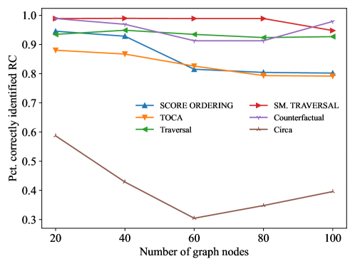
Figure 1: True positive rate of the compared algorithms in identifying the root cause with known structural assignments against the strength of the perturbation injected to the root cause.

When comparing the performance we should however keep in mind that Counterfactual requires the SCM, while Traversal and SMOOTH TRAVERSAL require only the causal graph, this is a clear disadvantage of Counterfactual against the other two algorithms. In addition, SMOOTH TRAVERSAL does not have a free parameter (thresholding scores), which Traversal does. Both SCORE ORDERING and TOCA have similar performance, but SCORE ORDERING does not even require information of the causal graph, whereas TOCA does. Nevertheless, it has the advantage over all others (except Counterfactual), that the inferred gap of log probabilities witnesses a true causal contribution, which is not the case for other methods since upstream anomalies may not be causally responsible for the target anomaly (as argued in Section 3).

We have also tried our algorithms on the ’PetShop dataset’ [29], where the task is to infer the root cause of performance drops in a cloud-based application. This presents a challenging task due to high missingness, low sample sizes, and near-constant variables. Furthermore, the causal ground truth is only partially known if one accepts that the inverted call graph (showing which services call which in the application) is a proxy for the causal graph. The results are shown in Appendix B.3, SMOOTH TRAVERSAL and SCORE ORDERING perform well, while TOCA fails, probably because it relies heavily not only on the causal graph but also on the SCM.

6 Conclusions

Without challenging the approach of [23] for a clean definition of root cause and its quantitative contribution, we have explored several directions in which the practical limitations of the corresponding algorithm provided in DoWhy [47] can be mitigated without sacrificing too much of its theoretical justification: First, by avoiding rung 3 causal models and high computational load, second by avoiding estimation of conditional probabilities, and third by not even relying on the causal DAG.

Appendix A Proofs

A.1 Proof of Proposition 2.1

With the event $E$ as in Eq. 3 and $C^{\pi}(j)$ as in Eq. 8 we have

$$C^{\pi}(j)=\log\frac{P(E|{\bf N}_{\pi>j~{}\cup\left\{j\right\}}={\bf n}_{\pi>j~{}\cup\left\{j\right\}})}{P(E|{\bf N}_{\pi>j}={\bf n}_{\pi>j})}\overset{i}{=}\log\frac{P(E|{\bf X}_{\pi>j~{}\cup\left\{j\right\}}={\bf x}_{\pi>j~{}\cup\left\{j\right\}})}{P(E|{\bf X}_{\pi>j}={\bf x}_{\pi>j})}\overset{ii}{=}\log\frac{P(E|do({\bf X}_{\pi>j~{}\cup\left\{j\right\}}={\bf x}_{\pi>j~{}\cup\left\{j\right\}})}{P(E|do({\bf X}_{\pi>j}={\bf x}_{\pi>j}))}.$$ (20)

(i) and (ii) are seen as follows:

$$P(E|{\bf N}_{\mathcal{I}})=P(E|{\bf X}_{\mathcal{I}}))=P(E|do({\bf X}_{\mathcal{I}})).$$ (21)

The first equality in Eq. 21 follows from $X_{n}\perp I_{\mathcal{I}}\,|{\bf N}_{\mathcal{I}}$ and because ${\bf X}_{\mathcal{I}}$ is a function of ${\bf N}_{\mathcal{I}}$. The second one follows because conditioning on all ancestors blocks all backdoor paths. Note that since $\pi$ is a reverse topological ordering of the nodes all $\pi>j$ are ancestors of $j$.

A.2 Proof of Lemma 3.1

$$C(\mathcal{R}|\bar{{\mathcal{S}}}) =\log q({\mathcal{S}}\cup\mathcal{R})-\log q({\mathcal{S}})$$

$$=\left(\log q({\mathcal{S}}\cup\mathcal{R})-\log q({\mathcal{S}}\cup\mathcal{R}\setminus\left\{j_{1}\right\})\right)+\left(\log q({\mathcal{S}}\cup\mathcal{R}\setminus\left\{j_{1}\right\})-\log q({\mathcal{S}}\cup\mathcal{R}\setminus\left\{j_{1},j_{2}\right\}\right))+\ldots$$

$$+\left(\log q({\mathcal{S}}\cup\left\{j_{k}\right\})-\log q({\mathcal{S}})\right)=\sum_{i=1}^{k}C(j_{i}|\overline{{\mathcal{S}}\cup\mathcal{R}\setminus\{j_{1},\dots,j_{i}\}}).$$

A.3 Proof of Proposition 3.2

By definition we have that

$$C(R|\bar{S})=\log\frac{P(E|{\bf N}_{R}={\bf n}_{R},{\bf N}_{S}={\bf n}_{S})}{P(E|{\bf N}_{S}={\bf n}_{S})},$$

and we use $P(E|{\bf n}_{S})$ instead of $P(E|{\bf N}_{S}={\bf n}_{S})$ when it is clear from the context.

Further, $C(R|\bar{S})$ is actually a function of ${\bf n}_{R}$ and ${\bf n}_{S}$. For fixed ${\bf n}_{S}$, define the set $B:=\{{\bf n}_{R}\,|C(R|\bar{S})\geq\alpha\}$. It can equivalently be described by

$$B=\{{\bf n}_{R}\,|\log\frac{P(E|{\bf n}_{R},{\bf n}_{S})}{P(E|{\bf n}_{S})}\geq\alpha\}=\{{\bf n}_{R}\,|P(E|{\bf n}_{R},{\bf n}_{S})\geq P(E|{\bf n}_{S})\cdot e^{\alpha}\}.$$

We thus have

$$P(E|{\bf n}_{R}\in B,{\bf n}_{S})\geq P(E|{\bf n}_{S})\cdot e^{\alpha}.$$

Hence,

$$\frac{P(E,{\bf n}_{R}\in B|{\bf n}_{S})}{P({\bf n}_{R}\in B|{\bf n}_{S})}\geq P(E|{\bf n}_{S})\cdot e^{\alpha}.$$

Using

$$P(E|{\bf n}_{S})\geq P(E,{\bf n}_{R}\in B|{\bf n}_{S})$$

we obtain

$$P({\bf n}_{R}\in B|{\bf n}_{S})\leq e^{-\alpha}.$$

A.4 Proof of Lemma 3.3

$$C(\bar{\mathcal{S}}\,|\,{\mathcal{S}})=\log\frac{q(\bar{\mathcal{S}})}{q(\emptyset)}\overset{i}{=}\log q(\bar{\mathcal{S}})+S(x_{n})$$

$$=\log P(E\,|\,{\bf n}_{\bar{{\mathcal{S}}}})+S(x_{n})$$

$$\Rightarrow P(E\,|\,{\bf n}_{\bar{{\mathcal{S}}}})=e^{C(\bar{{\mathcal{S}}}|{\mathcal{S}})-S(x_{n})}\overset{ii}{=}e^{-C(S|\bar{S})}.$$

were $(i)$ follows from $S(x_{n})=-\log P(E)$ and $(ii)$ follows from the fact that $S(x_{n})=\sum_{i}C(\mathcal{I}_{i}\,|\,.)$ as long as $\underset{i}{\cup}~{}\mathcal{I}_{i}=\mathcal{U}$.

A.5 Proof of Lemma 3.5

The proof simply follows by using Hoeffding’s bound 3.5 together with union bound, if $k$ data points are used for estimation of each $P(E\,|\,{\bf n}_{I^{\pi<i}})$, we have based on Hoeffding’s bound for each $i$ that:

$$P\left(|\hat{P}(E\,|\,{\bf n}_{I^{\pi<i}})-P(E\,|\,{\bf n}_{I^{\pi<i}})|<\delta\right)>1-2e^{-2k\delta^{2}},$$

From union bound we have that it simultaneously holds for all $i$ with probability at least $1-2ne^{-2k\delta^{2}}$. To have $1-2ne^{-2k\delta^{2}}>1-\alpha$ we should have:

$$2ne^{-2k\delta^{2}}<\alpha\Rightarrow k>\frac{\log\frac{2n}{\alpha}}{2\delta^{2}}$$

A.6 Proof of Lemma 4.2

$$P\left\{S(Y)\geq S(y)|X=x\right\}$$

$$= P\{S(Y)\geq S(y)|S(X)=S(x)\}$$

$$\leq P\{S(Y)\geq S(y)|S(X)\geq S(x)\}$$

$$\leq \frac{P\{S(Y)\geq S(y)\}}{P\{S(X)\geq S(x))\}}=\frac{e^{-S(y)}}{e^{-S(x)}}.$$

The first equality uses injectivity, and the second inequality monotonicity (see Subsection 4.1. The third one follows from $P(A|B)\leq P(A)/P(B)$ for any two events $A,B$.

A.7 Proof of Lemma 4.3

Assume without loss of generality that $X_{1},\dots,X_{n}$ is a topological ordering of the DAG. Then $S(X_{i}|X_{1},\dots,X_{i-1})=S(X_{i}|Pa_{i})$ holds due to the local Markov condition. Since $S(X_{j}|Pa_{j}=pa_{j})$ has density $e^{-s}$ for all $pa_{i}$, also $S(X_{i}|X_{1}=x_{1},\dots,X_{i-1}=x_{i-1})$ has density $e^{-s}$ for all $x_{1},\dots,x_{i-1}$. Hence, $S(X_{i}|Pa_{i})$ is independent of $X_{1},\dots,X_{i-1}$.

A.8 Proof of Lemma 4.4

The proof follows from a minor modification of the proof of Lemma 1 in [45] by replacing $n$ with $n-1$.

A.9 Proof of Theorem 4.5

The theorem is a direct result of Lemma 4.3 and Lemma 4.4.

A.10 Proof of Theorem 4.6

$$P(E_{i}|Pa_{i}=pa_{i}) \leq P(E_{i}|E_{Pa_{i}^{1}},\dots,E_{Pa_{i}^{k}})$$

$$\leq \frac{P(E_{i})}{P(E_{Pa_{i}^{1}},\dots,E_{Pa_{i}^{k}})}$$

$$\leq \frac{P(E_{i})}{P(E_{Pa_{i}^{1}})\cdots P(E_{Pa^{k}_{i}})}.$$

Recalling that anomaly scores are non-negative, we thus obtain:

$$S(x_{i}|pa_{i})\geq|S(x_{i})-\sum_{l=1}^{k}S(pa^{l}_{i})|_{+},$$

with the notation $|a|:=(a+|a|)/2$. Hence, we obtain a lower bound for $s_{cum}$:

$$s_{cum}\geq\sum_{i\neq j}|S(x_{i})-\sum_{l}S(pa^{l}_{i})|_{+}=:\hat{s}_{cum}.$$ (22)

Appendix B Experimental details and further experiments

B.1 Experimental details

To generate an SCM for the experiments in Section. 5 (see Fig. 1), we first uniformly sample between 10 and 20 root nodes (20% to 40% of the total nodes of the graph) and uniformly assign to each either a standard Gaussian, uniform or mixture of Gaussians as its noise distribution. As a second step, we recursively sample non-root nodes. Non-root nodes need not be sink nodes. The number of parent nodes that each non-root node is conditioned on is randomly chosen following a distribution that assigns a lower probability to a higher number of parents. In total, the causal graph is composed of 50 nodes. The parametric forms of the structural equations are randomly assigned to be either a simple feed-forward neural network with a probability of 0.8 (to account for non-linear models) and a linear model. The feed-forward neural network has three layers (input layer, hidden layer, and output layer) where the hidden layer has a number of nodes chosen randomly between 2 and 100. All the parameters of the neural network are sampled from a uniform distribution between -5 and 5. For the linear model, we sample the coefficients of the linear model from a uniform distribution between -1 and 1 and set the intercept to 0. In both cases, we use additive Gaussian noise as the relation between the noise and the variables.

To generate data for the non-anomalous regime we sample the noise of each of the variables and propagate the noise forward using the previously sampled structural equations. As mentioned in the main text, to produce anomalous data we choose a root cause at random from the list of all nodes and a target node from the set of its descendants (including itself). Then we sample the noise of all variables and modify the noise of the root cause by adding $x$ standard deviations, where $x\in\{2,2.1,\dots,3\}$, and propagate the noises through the SCM to obtain a realization of each variable. We repeat this process 100 times for each $x$ value added to the standard deviation and consider the algorithm successful if its result coincides with the chosen root cause.

Figure 2: Runtimes of the algorithms for the experiment in Fig. 1. The vertical axis in log scale.

B.2 Further experiments by varying the number of nodes in the graph

We also run experiments by fixing the number of standard deviations added ($x$ in Section. 5) to 3 and varying the number of nodes in the SCM. The number of nodes we run the experiments on is $\{20,40,60,80,100\}$. We see in Fig. 3 that the performance for Traversal, SMOOTH TRAVERSAL, and Counterfactual does not change much for different graph sizes, whereas the quality of TOCA and SCORE ORDERING decreases slightly for larger graph sizes. Circa, on the other hand, has worse performance for an intermediate number of nodes but the quality increases as the graph gets larger.

Figure 3: True positive rate of the compared algorithms in identifying the root cause with known structural assignments.

Fig. 4 shows the runtime of all the algorithms for an SCM with 100 variables (and added standard deviation 3). The only qualitative change between this Figure and Fig. 2 is that SCORE ORDERING is slightly faster than TOCA.

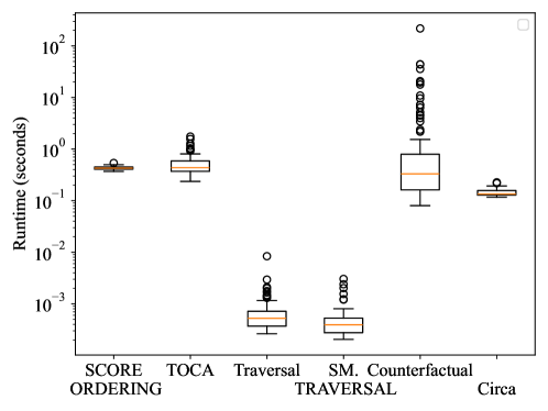
Figure 4: Runtimes of the algorithms for SCM with 100 nodes. The vertical axis is truncated to see a clearer difference in the runtimes.

B.3 PetShop dataset

[29] introduces a dataset specifically designed for evaluating root cause analyses in microservice-based applications. The dataset includes 68 injected performance issues, which increase latency and reduce availability throughout the system. In addition to the approaches evaluated by the authors, reproduced below, we evaluated our algorithms in both top-1 recall (Table. 1) and top-3 recall (Table. 2).

Table 1: Top-1 recall

		graph given			graph not given			this paper
traffic	metric	traversal	circa	counter-	$\epsilon$-diagnosis	rcd	correlation	score	TOCA	smooth
scenario				factual				ordering		traversal
low	latency	0.57	0.36	0.36	0.00	0.07	0.43	0.29	0.00	0.21
low	availability	0.50	0.42	0.00	0.00	0.58	0.75	0.42	0.00	0.33
high	latency	0.57	0.50	0.57	0.00	0.00	0.64	0.14	0.00	0.14
high	availability	0.33	0.00	0.00	0.00	0.00	0.83	0.17	0.00	0.00
temporal	latency	1.00	0.75	0.38	0.12	0.25	0.62	0.25	0.00	0.25
temporal	availability	0.38	0.38	0.00	0.00	0.50	0.62	0.38	0.00	0.13

Table 2: Top-3 recall

		graph given			graph not given			this paper
traffic	metric	traversal	circa	counter-	$\epsilon$-diagnosis	rcd	correlation	score	TOCA	smooth
scenario				factual				ordering		traversal
low	latency	0.57	0.86	0.71	0.00	0.21	0.57	0.71	0.21	0.36
low	availability	1.00	1.00	0.42	0.00	0.75	0.92	0.92	0.00	0.67
high	latency	0.79	1.00	0.86	0.00	0.07	0.79	0.57	0.00	0.57
high	availability	1.00	0.00	0.00	0.33	0.00	0.92	0.17	0.00	0.67
temporal	latency	1.00	1.00	0.50	0.12	0.75	0.75	0.75	0.00	0.75
temporal	availability	1.00	1.00	0.25	1.00	0.12	0.75	0.75	0.00	0.50

References

- [1] S Wibisono, MT Anwar, Aji Supriyanto, and IHA Amin. Multivariate weather anomaly detection using dbscan clustering algorithm. In Journal of Physics: Conference Series, volume 1869, page 012077. IOP Publishing, 2021.
- [2] Eric V Strobl and Thomas A Lasko. Identifying patient-specific root causes with the heteroscedastic noise model. Journal of Computational Science, 72:102099, 2023.
- [3] Eric V Strobl. Counterfactual formulation of patient-specific root causes of disease. Journal of Biomedical Informatics, page 104585, 2024.
- [4] Gian Antonio Susto, Matteo Terzi, and Alessandro Beghi. Anomaly detection approaches for semiconductor manufacturing. Procedia Manufacturing, 11:2018–2024, 2017.
- [5] Jellis Vanhoeyveld, David Martens, and Bruno Peeters. Value-added tax fraud detection with scalable anomaly detection techniques. Applied Soft Computing, 86:105895, 2020.
- [6] Sanjiv Das, Richard Stanton, and Nancy Wallace. Algorithmic fairness. Annual Review of Financial Economics, 15:565–593, 2023.
- [7] Dongjie Wang, Zhengzhang Chen, Jingchao Ni, Liang Tong, Zheng Wang, Yanjie Fu, and Haifeng Chen. Hierarchical graph neural networks for causal discovery and root cause localization. arXiv preprint arXiv:2302.01987, 2023.
- [8] Cheng-Ming Lin, Ching Chang, Wei-Yao Wang, Kuang-Da Wang, and Wen-Chih Peng. Root cause analysis in microservice using neural granger causal discovery. arXiv preprint arXiv:2402.01140, 2024.
- [9] Dewei Liu, Chuan He, Xin Peng, Fan Lin, Chenxi Zhang, Shengfang Gong, Ziang Li, Jiayu Ou, and Zheshun Wu. Microhecl: high-efficient root cause localization in large-scale microservice systems. In Proceedings of the 43rd International Conference on Software Engineering: Software Engineering in Practice, ICSE-SEIP ’21, page 338–347. IEEE Press, 2021.
- [10] Azam Ikram, Sarthak Chakraborty, Subrata Mitra, Shiv Saini, Saurabh Bagchi, and Murat Kocaoglu. Root cause analysis of failures in microservices through causal discovery. Advances in Neural Information Processing Systems, 35:31158–31170, 2022.
- [11] Huasong Shan, Yuan Chen, Haifeng Liu, Yunpeng Zhang, Xiao Xiao, Xiaofeng He, Min Li, and Wei Ding. -diagnosis: Unsupervised and real-time diagnosis of small-window long-tail latency in large-scale microservice platforms. In The World Wide Web Conference, pages 3215–3222, 2019.
- [12] Meng Ma, Jingmin Xu, Yuan Wang, Pengfei Chen, Zonghua Zhang, and Ping Wang. Automap: Diagnose your microservice-based web applications automatically. In Proceedings of The Web Conference 2020, pages 246–258, 2020.
- [13] Douglas M Hawkins. Identification of outliers, volume 11. Springer, 1980.
- [14] Varun Chandola, Arindam Banerjee, and Vipin Kumar. Anomaly detection: A survey. ACM computing surveys (CSUR), 41(3):1–58, 2009.
- [15] Charu C Aggarwal. An introduction to outlier analysis. Springer, 2017.
- [16] Ane Blázquez-García, Angel Conde, Usue Mori, and Jose A Lozano. A review on outlier/anomaly detection in time series data. ACM Computing Surveys (CSUR), 54(3):1–33, 2021.
- [17] Leman Akoglu. Anomaly mining: Past, present and future. In Proceedings of the 30th ACM International Conference on Information & Knowledge Management, pages 1–2, 2021.
- [18] Edwin M Knorr and Raymond T Ng. Finding intensional knowledge of distance-based outliers. In Vldb, volume 99, pages 211–222, 1999.
- [19] Barbora Micenková, Raymond T Ng, Xuan-Hong Dang, and Ira Assent. Explaining outliers by subspace separability. In 2013 IEEE 13th international conference on data mining, pages 518–527. IEEE, 2013.
- [20] Ninghao Liu, Donghwa Shin, and Xia Hu. Contextual outlier interpretation. arXiv preprint arXiv:1711.10589, 2017.
- [21] Meghanath Macha and Leman Akoglu. Explaining anomalies in groups with characterizing subspace rules. Data Mining and Knowledge Discovery, 32:1444–1480, 2018.
- [22] Nikhil Gupta, Dhivya Eswaran, Neil Shah, Leman Akoglu, and Christos Faloutsos. Beyond outlier detection: Lookout for pictorial explanation. In Machine Learning and Knowledge Discovery in Databases: European Conference, ECML PKDD 2018, Dublin, Ireland, September 10–14, 2018, Proceedings, Part I 18, pages 122–138. Springer, 2019.
- [23] Kailash Budhathoki, Lenon Minorics, Patrick Bloebaum, and Dominik Janzing. Causal structure-based root cause analysis of outliers. In Kamalika Chaudhuri, Stefanie Jegelka, Le Song, Csaba Szepesvari, Gang Niu, and Sivan Sabato, editors, Proceedings of the 39th International Conference on Machine Learning, volume 162 of Proceedings of Machine Learning Research, pages 2357–2369. PMLR, 17–23 Jul 2022.
- [24] Dongjie Wang, Zhengzhang Chen, Jingchao Ni, Liang Tong, Zheng Wang, Yanjie Fu, and Haifeng Chen. Interdependent causal networks for root cause localization. In Proceedings of the 29th ACM SIGKDD Conference on Knowledge Discovery and Data Mining, pages 5051–5060, 2023.
- [25] Mingjie Li, Zeyan Li, Kanglin Yin, Xiaohui Nie, Wenchi Zhang, Kaixin Sui, and Dan Pei. Causal inference-based root cause analysis for online service systems with intervention recognition. In Proceedings of the 28th ACM SIGKDD Conference on Knowledge Discovery and Data Mining, pages 3230–3240, 2022.
- [26] Dongjie Wang, Zhengzhang Chen, Yanjie Fu, Yanchi Liu, and Haifeng Chen. Incremental causal graph learning for online root cause analysis. In Proceedings of the 29th ACM SIGKDD Conference on Knowledge Discovery and Data Mining, pages 2269–2278, 2023.
- [27] Pengfei Chen, Yong Qi, Pengfei Zheng, and Di Hou. Causeinfer: Automatic and distributed performance diagnosis with hierarchical causality graph in large distributed systems. In IEEE INFOCOM 2014 - IEEE Conference on Computer Communications, pages 1887–1895, 2014.
- [28] JinJin Lin, Pengfei Chen, and Zibin Zheng. Microscope: Pinpoint performance issues with causal graphs in micro-service environments. In International Conference on Service Oriented Computing, 2018.
- [29] Michaela Hardt, William Orchard, Patrick Blöbaum, Shiva Kasiviswanathan, and Elke Kirschbaum. The petshop dataset – finding causes of performance issues across microservices, 2023.
- [30] Yu Gan, Mingyu Liang, Sundar Dev, David Lo, and Christina Delimitrou. Sage: practical and scalable ml-driven performance debugging in microservices. In Proceedings of the 26th ACM International Conference on Architectural Support for Programming Languages and Operating Systems, ASPLOS ’21, page 135–151, New York, NY, USA, 2021. Association for Computing Machinery.
- [31] Azam Ikram. Sock-shop data. https://github.com/azamikram/rcd/tree/master/sock-shop-data, 2023.
- [32] Amin Jaber, Murat Kocaoglu, Karthikeyan Shanmugam, and Elias Bareinboim. Causal discovery from soft interventions with unknown targets: Characterization and learning. In H. Larochelle, M. Ranzato, R. Hadsell, M.F. Balcan, and H. Lin, editors, Advances in Neural Information Processing Systems, volume 33, pages 9551–9561. Curran Associates, Inc., 2020.
- [33] Nicola Gnecco, Nicolai Meinshausen, Jonas Peters, and Sebastian Engelke. Causal discovery in heavy-tailed models. The Annals of Statistics, 49(3):1755 – 1778, 2021.
- [34] Carlos Améndola, Benjamin Hollering, Seth Sullivant, and Ngoc Tran. Markov equivalence of max-linear Bayesian networks. In Cassio de Campos and Marloes H. Maathuis, editors, Proceedings of the Thirty-Seventh Conference on Uncertainty in Artificial Intelligence, volume 161 of Proceedings of Machine Learning Research, pages 1746–1755. PMLR, 27–30 Jul 2021.
- [35] J. Pearl and J. Mackenzie. The book of why. Basic Books, USA, 2018.
- [36] J. Pearl. Causality. Cambridge University Press, 2000.
- [37] Kun Zhang, Zhikun Wang, Jiji Zhang, and Bernhard Schölkopf. On estimation of functional causal models: general results and application to the post-nonlinear causal model. ACM Transactions on Intelligent Systems and Technology (TIST), 7(2):1–22, 2015.
- [38] Julius Von Kügelgen, Abdirisak Mohamed, and Sander Beckers. Backtracking counterfactuals. In Mihaela van der Schaar, Cheng Zhang, and Dominik Janzing, editors, Proceedings of the Second Conference on Causal Learning and Reasoning, volume 213 of Proceedings of Machine Learning Research, pages 177–196. PMLR, 11–14 Apr 2023.
- [39] A. Balke and J. Pearl. Counterfactual probabilities: Computational methods, bounds, and applications. In R. Lopez D. Mantaras and D. Poole, editors, Uncertainty in Artifical Intelligence, volume 10. Morgan Kaufmann, San Mateo, 1994.
- [40] Akash Maharaj, Ritwik Sinha, David Arbour, Ian Waudby-Smith, Simon Z. Liu, Moumita Sinha, Raghavendra Addanki, Aaditya Ramdas, Manas Garg, and Viswanathan Swaminathan. Anytime-valid confidence sequences in an enterprise a/b testing platform. In Companion Proceedings of the ACM Web Conference 2023, WWW ’23 Companion, page 396–400, New York, NY, USA, 2023. Association for Computing Machinery.
- [41] Dominik Janzing, Patrick Blöbaum, Atalanti A Mastakouri, Philipp M Faller, Lenon Minorics, and Kailash Budhathoki. Quantifying intrinsic causal contributions via structure preserving interventions. In International Conference on Artificial Intelligence and Statistics, pages 2188–2196. PMLR, 2024.
- [42] Yoshua Bengio, Tristan Deleu, Nasim Rahaman, Rosemary Ke, Sébastien Lachapelle, Olexa Bilaniuk, Anirudh Goyal, and Christopher Pal. A meta-transfer objective for learning to disentangle causal mechanisms. arXiv preprint arXiv:1901.10912, 2019.
- [43] B. Schölkopf, F. Locatello*, S. Bauer, N. R. Ke, N. Kalchbrenner, A. Goyal, and Y. Bengio. Toward causal representation learning. Proceedings of the IEEE, 109(5):612–634, 2021.
- [44] Judea Pearl. Sufficient causes: On oxygen, matches, and fires. Journal of Causal Inference, 7(2), 2019.
- [45] Dominik Janzing, Kailash Budhathoki, Lenon Minorics, and Patrick Blöbaum. Causal structure based root cause analysis of outliers. arxiv:1912.02724, 2019.
- [46] R. A. Fisher. Statistical Methods for Research Workers. Oliver and Boyd, 1925.
- [47] Patrick Blöbaum, Peter Götz, Kailash Budhathoki, Atalanti A. Mastakouri, and Dominik Janzing. Dowhy-gcm: An extension of dowhy for causal inference in graphical causal models, 2022.