padding=1.0ex,1.0ex, 1.0ex, 1.0ex, margin=1em,0.0em,0em

Compilation Quotient (CQ): A Metric for the Compilation Hardness of Programming Languages

Vince Szabó TU DelftNetherlands V.Szabo-2@student.tudelft.nl ,  Dominik Winterer ETH ZurichDepartment of Computer ScienceSwitzerland dominik.winterer@inf.ethz.ch  and  Zhendong Su ETH ZurichDepartment of Computer ScienceSwitzerland zhendong.su@inf.ethz.ch

Abstract.

Today’s programmers can choose from an exceptional range of programming languages, each with its own traits, purpose, and complexity. A key aspect of a language’s complexity is how hard it is to compile programs in the language. While most programmers have an intuition about compilation hardness for different programming languages, no metric exists to quantify it. We introduce the compilation quotient (CQ), a metric to quantify the compilation hardness of compiled programming languages. The key idea is to measure the compilation success rates of programs sampled from context-free grammars. To this end, we fairly sample over 12 million programs in total. CQ ranges between 0 and 100, where 0 indicates that no programs compile, and 100 means that all programs compile. Our findings on 12 popular compiled programming languages show high variation in CQ. C has a CQ of 48.11, C++ has 0.60, Java has 0.27 and Haskell has 0.13. Strikingly, Rust’s CQ is nearly 0, and for C, even a large fraction of very sizable programs compile. We believe CQ can help understand the differences of compiled programming languages better and help language designers.

1. Introduction

Programming languages profoundly influence how we build software. Each programming language has its own characteristic traits, purposes, infrastructure, and complexity. One key aspect of a language’s complexity is how hard it is to produce valid programs $P$ in the language. If the language is compiled, an ahead-of-time compiler decides whether $P$ is valid, produces an executable in case of success, and rejects the program with an error otherwise. Rejected programs frustrate programmers, leading to reduced productivity, failed or abandoned projects, etc. While most programmers have an intuition of the hardness of writing compiling programs in different programming languages, no metric exists to quantify it. Without a metric, language designers rely solely on user experiences, which can be valuable but are also potentially biased and contradictory. Moreover, without a metric, learning from historical languages’ benefits and flaws is difficult. However, realizing a metric to quantify the compilation hardness of different languages is challenging since it requires inferring compilation hardness on the (infinite) space of all programs.

Compilation Quotient

We propose the compilation quotient (CQ), a metric for the compilation hardness of programming languages. The key idea is to measure CQ for programming language $\mathit{PL}$ by sampling programs from context-free grammars for $\mathit{PL}$. Concretely, the CQ of $\mathit{PL}$ is the percentage of accepted programs over the total number of sampled programs for $\mathit{PL}$. CQ ranges between 0 and 100, where 0 indicates that no programs compile, and 100 means that all programs compile. We compute the CQ for a given language $\mathit{PL}$ by the following steps: (1) translate the context-free grammar into algebraic datatypes, (2) sample a large number of programs using off-the-shelf property-based tester FEAT, (3) forward each of these programs to a $PL$ compiler and track the results, and (4) compute the CQ by dividing the number of compiling samples by the number of total samples. We obtain the context-free grammars for the languages from the repository of ANTLR, the parser generator (Parr et al., 2014). To sample programs of diverse sizes, we use a bucket-based algorithm with lower and upper bounds on program size (see Section 2.4). We use the most popular compiler for each language, e.g., gcc for C, g++ for C++, rustc for Rust, and ghc for Haskell.

Results & Insights

We compute the CQs of twelve popular compiled programming languages. Our findings show high variation in CQ (see Fig. 1(a)). The language with the highest CQ is C. It has a CQ of 48.11 leading by a large margin over all other languages. C++ has a CQ of 0.60, Java has a CQ of 0.27 and Haskell has a CQ of 0.13. Other interesting observations include that the most popular object-oriented programming languages all rank high in the CQ ranking (i.e., C#, Java, and C++). Besides, we also investigate the percentage of valid programs as program size increases (see Fig. 1(b)). Strikingly, for C, the percentage of valid C programs converges to a strictly positive value as program size increases, unlike the distributions of all other languages which drop to zero instead. Complementing quantitative results, we analyze sample programs from each language, identify notable features, and discuss their effect on CQ, presenting patterns between different languages.

#	Language	CQ
1	C	48.110
2	Erlang	6.511
3	C#	1.691
4	C++	0.598
5	Kotlin	0.308
6	Java	0.265
7	Haskell	0.128
8	Fortran	0.033
9	COBOL	0.032
10	Go	0.030
11	Swift	0.018
12	Rust	0.0004

(a)

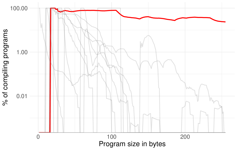
(b)

Figure 1. (a) CQ-ranking of twelve popular compiled languages, and (b) C’s divergence.

Main Contributions

We make the following main contributions:

• We introduce the compilation quotient (CQ), a metric for the compilation hardness of programming languages;

• We propose a framework to compute CQs, including a sampling algorithm and a practical tool cq-test for sampling more than 12 million programs;

• We calculate CQ for twelve popular compiled programming languages including C, C++, Java, C#, Kotlin, Haskell, and Rust;

• We conduct in-depth analyses on the distribution of valid programs w.r.t. program size, how various language features affect CQ, discuss the meaning of the metric, etc.

We will open-source source cq-test and plan to submit it to artifact evaluation. Moreover, cq-test and the experimental data is attached to this submission.

Structure of the paper

The paper realizes an empirical study. First, we describe its setup (Section 2) including programming languages, sampling etc., then we describe the results (see Section 3) and interpret them (Section 4). We discuss the implications of CQ (Section 5), survey related work (Section 6), and close with a conclusion (Section 7).

2. Empirical Setup

We first describe our selection of compiled programming languages (Section 2.1) including their context-free grammars (Section 2.2). Second, we introduce the compilation quotient (CQ), a metric for the compilation hardness of programming languages (Section 2.3). Finally, we describe algorithms for computing CQ (Section 2.4) and describe additional setup details (Section 2.5).

2.1. Compiled Programming Languages

We consider compiled programming languages satisfying the following three criteria: (1) the language’s source code is written in a human-readable, high-level language,(2) the language’s source code is transformed by an ahead-of-time compiler to realize an executable and (3) the executable can be executed directly on a computer or indirectly by another runtime system. For this work, we restrict ourselves to compiled languages as they have a clear distinction between semantic errors and runtime errors, unlike interpreted languages or hybrids. We make a selection of compiled programming languages including those in the top 20 of the TIOBE index (see Fig. 2(a)), the leading language popularity metric. For a programming language $\mathit{PL}$, the index can be thought of as the percentage of $\mathit{PL}$’s weighted hits w.r.t. the total weighted search hits of all programming languages in major web search engines including Google, Bing, Baidu, Wikipedia, and YouTube. C, for example, has the highest TIOBE index (11.27%) which puts it at the top of the ranking. Besides the compiled languages in the top 20 of TIOBE, we consider Haskell because of its importance to the PL community, and COBOL and Erlang for historical importance. We exclude non-textual languages.

#	Language	Score
2	C	11.27%
3	C++	10.65%
4	Java	9.49%
5	C#	7.31%
7	Visual Basic	2.22%
11	Fortran	1.28%
12	Go	1.19%
15	Delphi/Object Pascal	1.02%
16	Swift	1.00%
17	Rust	0.97%
20	Kotlin	0.90%
21	COBOL	0.88%
28	Haskell	0.65%
51 - 100	Erlang	¡ 0.24%

(a)

Grammar	# nont.	# ter.	# prod.
C	83	118	163
C++	188	141	305
Java	123	122	213
C#	207	162	322
Fortran	335	177	377
Go	103	70	115
Swift	307	170	320
Rust	194	108	407
Kotlin	150	142	163
COBOL	590	558	280
Haskell	223	132	248
Erlang	122	8	129

(b)

Figure 2. (a) Selected TIOBE score of programming languages with rank (#) as of September 2023. (b) ANTLR grammar statistics: nonterminals (# nont.), terminals (# ter.) and production counts (# prod.). Grayed: For Visual Basic and Delphi/Object Pascal there were no suitable ANTLR grammars.

2.2. Grammars for Programming Languages

For each chosen programming language $\mathit{PL}$, we use a context-free grammar from the ANTLR grammar repository.  If there are multiple grammars for a programming language $\mathit{PL}$, we choose the grammar with the newest version of $\mathit{PL}$. We aim at following $\mathit{PL}$’s official language specification as closely as possible, without sampling too many equivalent programs. To that end, we modify each grammar as follows: (1) we bound the number of identifiers (i.e. variables) to two, (2) we restrict the number of literals per datatype to one, e.g., ”string” for strings, ”$42$” for integers, ”$123.4$” for doubles etc., except for booleans for which we allow both ”true” and ”false”, (3) we create a single entry point, usually a main function, with all statements, and (4) we fix orders of modifiers to avoid combinatorial explosions. Besides these changes, we describe the following further changes:

C.:

The grammar for C realizes the C11 standard (ISO/IEC, 2011). The grammar includes non-standard extensions, and datatypes for processors supporting Single Instruction Multiple Data (SIMD). We remove all these extensions and additionally remove inline assembly.

:

C++.:

The grammar for C++ realizes the C++14 standard (International Organization for Standardization, 2014). We remove attributes, user-defined literals, and alternative operator representations. Similar to C, we remove inline assembly.

:

C#.:

The grammar for C# realizes version 6 of the language (Microsoft, 2015). We remove string interpolation. Furthermore, we remove unsafe modifiers as these never compile without special compiler flags. Likewise, we remove pointer operations since these are only valid in an unsafe context.

:

Fortran.:

The Fortran grammar realizes the 1990 standard of the language (for, 1991). We reduce duplicate programs by forcing uppercase keywords, separable keywords to be written together (e.g. GOTO instead of GO TO), and operators to be in their text representation (e.g. .NE. instead of /=). We restrict labels to two values ($100$ and $200$) and restrict literals to those supported by GFortran. We remove IMPLICIT statements except for IMPLICIT NONE.  We further remove import statements for external files. Finally, we remove format statements.

:

Java, Go.:

For the Java and Go grammars, no language-specific modifications were needed. The Java grammar realizes the Java 17  (Gosling et al., 2021) and the Go grammar realizes version 1.20 (Authors, 2023).

:

Swift.:

The Swift grammar realizes version 5.4 (Inc., 2021). We remove extended string literals, imports, availability conditions, conditional compilation statements, and attributes. We restrict the language to the plus and minus operators to avoid combinatorial explosion. We restrict implicit parameter names to $0 and $1. As the language has many modifiers, only valid for a specific declaration type, we tie modifiers to the correct construct.

:

Rust.:

The Rust grammar realizes version v1.60.0 (Team, 2022). We remove macros and attributes from the grammar. We also remove the extern modifier for functions.

:

Kotlin.:

The grammar for Kotlin realizes version 1.4 (JetBrains, 2023). We remove annotations, fix the order of modifiers, and tie modifiers to the correct declaration type.

:

COBOL.:

The grammar realizes COBOL 85 (ANSI X3J4 Committee, 1985). We removed null-terminated string literals, as well as CICS and SQL extensions. We define the entry point as a procedure division, optionally proceeded by a data division that may contain only a working-storage section. Only level numbers $01$, $02$, $66$, $77$ and $88$ are allowed in the working-storage section. To avoid duplicate programs, we force operators to use their character form instead of the more verbose syntax (e.g. $x>y$ instead of $x\texttt{\small GREATER THAN }y$). We force the usage of PICTURE instead of PIC.

:

Haskell.:

The grammar for Haskell realizes the 2010 version of the language (Marlow, 2009). We remove pragmas and qualified variable symbols. We remove constructor symbols as they can never be defined in programs generated by our setup. We restrict operator symbols to the plus and minus symbols, as otherwise, the number of permitted identifiers would be very large. As the entry point, we use:

⬇

main = return ()

func = ... where { varX = ...,... }

We permit func to be used as an identifier to enable generation of recursive programs.

:

Erlang.:

The grammar realizes Erlang 23.3 (Team, 2021). The only language-specific modification made was to reduce the number of atom literals to one, i.e., an_atom.

For Visual Basic (VB), there is only an ANTLR grammar for an outdated version 6.0 released in 1998. Compilers for this version were only available for Windows with an enterprise subscription. Moreover, for Delphi/Object Pascal there were no ANTLR grammar is available at all. We hence do not consider these two languages for our study.

2.3. Compilation Quotient

With the language grammars specified, we move on to the compilation quotient. First, we need a few basic, formal definitions, then present CQ and LCQ.

Definitions

We assume familiarity with context-free grammars (CFG) including derivations, terminals, nonterminals etc. Let $\mathit{PL}$ be a programming language, then we describe with $G_{\mathit{PL}}$ the associated context-free grammar of $\mathit{PL}$. We denote the filesize of program $P$ (in bytes) by $\mathit{size}(P)$. The induced language of a grammar $L(G_{\mathit{PL}})$ is the set of all words, i.e., programs, derivable from $G_{\mathit{PL}}$. For the semantically correct programs $P$ in $L(G_{\mathit{PL}})$, we write $\vdash P$. We further define $L_{S}(G_{\mathit{PL}})=\{P\in L(G_{\mathit{PL}})\leq S\}$ as the bounded language of $G_{\mathit{PL}}$ for a fixed size bound $S$.

Definition 0 (Compilation Quotient).

The compilation quotient (CQ) is defined as follows:

$$\mathsf{\bf CQ}(\mathit{PL})=\frac{|\{P\in L_{S}(G_{\mathit{PL}})\mid\ \vdash P\}|}{|\{P\in L_{S}(G_{\mathit{PL}})\}|}\times 100$$

where $\mathit{PL}$ is a programming language, $G_{\mathit{PL}}$ is a CFG for $\mathit{PL}$, and $S$ is a fixed size bound.

The intuition behind CQ is measuring the semantic constraints that a given PL imposes on the programmer. CQ ranges between $0$ and $100$. A CQ of $0$ for a language $\mathit{PL}$ indicates that all programs in $L(G_{\mathit{PL}})$ are semantically invalid. A CQ of $100$, on the other hand, means that all programs are semantically valid. In practice, we use the feedback of a compiler of $\mathit{PL}$ to determine the semantic validity of $\mathit{PL}$. For the computation of CQ, we will further assume programs of $\mathit{size}(P)$ less than 256 bytes. The CQ is a single number describing a given language as a whole. To analyze the distribution of programs, we introduce the local compilation quotient:

Definition 0 (Local Compilation Quotient).

The local compilation quotient (LCQ) is defined as follows:

$$\mathsf{\bf LCQ}(\mathit{PL},x,\varepsilon)=\frac{|\{P\in L(G_{\mathit{PL}})\wedge x-\varepsilon\leq size(P)\leq x+\varepsilon\mid\ \vdash P\}|}{|\{P\in L(G_{\mathit{PL}})\wedge x-\varepsilon\leq size(P)\leq x+\varepsilon\}|}\times 100$$

where $\mathit{PL}$ is a programming language, $G_{\mathit{PL}}$ is a context-free grammar for $\mathit{PL}$, $x$ is an integer indicating program size, and $\varepsilon$ is an integer indicating a window radius.

The LCQ is intuitively a decomposition of the CQ for the given language, describing the proportion of accepted programs at size $x$ and smoothing factor $\varepsilon$. For this paper, we will fix $\varepsilon=5$.

2.4. Computing Compilation Quotients

We now describe how to compute CQ. We first compile the context-free grammars to regular tree grammars, then describe the sampling algorithm along with an example.

Compiling context-free grammars to regular-tree grammars.

To sample programs from a context-free grammar, we compile the context-free grammar to a regular tree grammar, i.e., algebraic datatypes in a functional programming language such as Haskell. A context-free grammar $G=\langle N,\Sigma,P,S\rangle$ consists of nonterminals $N$, terminals $\Sigma$, productions $P$, and a start $S$ from $N$. A regular tree grammar $G^{\prime}=\langle N^{\prime},\Sigma^{\prime},P^{\prime},S^{\prime}\rangle$ consists of nonterminals $N^{\prime}$, a ranked alphabet $\Sigma^{\prime}$, productions $P^{\prime}$ and a start symbol $S^{\prime}$. The elements in $\Sigma^{\prime}$ have constructors with arities where terminals are nullary. Intuitively, constructors of strictly positive arity represent tree patterns. Productions in $P^{\prime}$ have a single nonterminal on the left-hand side and symbols from $N^{\prime}$ and $\Sigma^{\prime}$ on their right-hand side. We compile a context-free grammar $G=\langle N,\Sigma,P,S\rangle$ into a regular tree grammar $G^{\prime}=\langle N^{\prime},\Sigma^{\prime},P^{\prime},S^{\prime}\rangle$ as follows: (1) we set $N^{\prime}=N$ and $S^{\prime}=S$, (2) we define $\Sigma^{\prime}$ as a superset of $\Sigma$ with constructors $C^{i}_{\mathit{lhs}}(.)$ in $\Sigma^{\prime}$ for every production with left-hand side $\mathit{lhs}$, and (3) for $P^{\prime}$, we append a constructor $C^{i}_{\mathit{lhs}}(.)$ to every production $p^{i}_{\mathit{lhs}}$ in $P$. The resulting regular-tree grammar is then converted into algebraic datatypes. We realize the compilation in about 1,000 lines of Python code. The script generates Haskell code for exhaustive enumerator FEAT (Duregard et al., 2012). By this we obtain an enumeration of programs $f_{\mathit{PL}}:\mathbb{N}\rightarrow L(G_{\mathit{PL}})$ as a mapping from natural numbers to programs of $\mathit{PL}$.

Interval sampling of programs.

We sample programs from an interval bounded by a minimum $a$ and maximum $b$ on filesize. Given a sample size $n$, we want to obtain samples from $S$.

$$S\subseteq\{P\in L(G_{\mathit{PL}})\ |\ \mathit{size}(P)\ \in[a,b)\}\hskip 11.38092ptI=\{i\ |\ \mathit{size}(f_{\mathit{PL}}(i))\in[a,b)\}$$

The set $I$ is an index set to generate elements in $S$. Moreover, indices $i_{a}=\min\{I\}$ and $i_{b}=\max\{I\}$ locate the programs at the bounds. We want the indices of $S$ to be evenly distributed within $I$, to accurately measure the distribution of programs within the interval. FEAT’s enumeration is monotonically increasing in the constructors. Montonicity is not guaranteed for filesize, i.e., for indices $i<j$ implies $\mathit{size}(f_{\mathit{PL}}(i))<\mathit{size}(f_{\mathit{PL}}(j))$ does often hold but is not guaranteed. This implies that finding $i_{a}$ requires exhaustively checking every index up to $i_{a}$, which is infeasible. Hence we use the approximations $i_{a}^{\prime}$ and $i_{b}^{\prime}$ for the boundaries of the interval. Our realization of the sampling algorithm is presented in Algorithm 1. The algorithm takes $n$, filesize bounds $a$ and $b$, and indices for $i_{a}^{\prime}$ and $i_{b}^{\prime}$ as its input. We obtain $i_{a}^{\prime}$ and $i_{b}^{\prime}$ from the procedure EstimateIndex (see 2). The procedure SampleProgramInterval returns the first index of a program of filesize $x$. We describe details on EstimateIndex in the next paragraph. After initialization (Line 2), the algorithm enters its main loop in which it remains until either $n$ samples were collected or it was unsucessful after $\mathit{max\_tries}$ attempts. For our experiments we set $\mathit{max\_tries}$ to 16. We next sample from the enumeration at evenly distributed indices between $i_{a}^{\prime}$ and $i_{b}^{\prime}$. We next remove programs that have an incorrect size (Line 6). As this step reduces our candidate sample set, we oversample by a factor of $\alpha$. We set $\alpha$ to $8$ as our default configuration. If there are exactly $n$ samples left after the filtering, the algorithm concludes. If there are too many samples, we randomly take $n$ without replacement (Line 8). If there are too few, we retry, adjusting $i_{a}^{\prime}$ and $i_{b}^{\prime}$ using a factor $\beta$ (Line 10), and increasing our sampling density to find more programs of the correct size. We set $\beta$ to be $2$. If SampleProgramInterval fails to find sufficient samples after $\mathit{max\_tries}$ attempts, it terminates returning the sample set.

1:function SampleProgramInterval($n$, $a$, $b$, $i_{a}^{\prime}$, $i_{b}^{\prime}$)

2:     $best\leftarrow\emptyset,step\leftarrow 0,start\leftarrow i_{a}^{\prime},end\leftarrow i_{b}^{\prime}$

3:     while $|best|<n\land step<max\_tries$ do

4:         $n^{\prime}\leftarrow\alpha\cdot n\cdot(step+1)$

5:         $curr\leftarrow\{f_{\mathit{PL}}(i)\>|\>n^{\prime}\text{evenly spaced i's from [start{}, end{}) }\}$

6:         $curr\leftarrow\{w\in curr\>|\>a\leq size(w)<b\}$

7:         if $|curr|>n$ then

8:              $curr\leftarrow\text{take $n$ elements from curr{} without replacement}$          

9:         $best\leftarrow max\_by\_size(curr,best)$

10:         $step\leftarrow step+1,start\leftarrow\frac{start}{\beta},end\leftarrow end*\beta$      

11:     return $best$

Algorithm 1 Sampling programs in a given size range

1:function EstimateIndex(x)

2:     $i\leftarrow 0,steps\_taken\leftarrow 0,step\leftarrow 0$

3:     while $size(f_{\mathit{PL}}(i))<x$ do $\triangleright$ Overestimate the index

4:         if $steps\_taken=step\_increase\_threshold$ then

5:              $step\leftarrow step+1,steps\_taken\leftarrow 0$          

6:         $i\leftarrow i+10^{step},steps\_taken\leftarrow steps\_taken+1$      

7:     if $size(f_{\mathit{PL}}(i))=x$ then

8:         return $i$      

9:     $steps\_taken\leftarrow 0,step\leftarrow 0$

10:     while $size(f_{\mathit{PL}}(i))>x$ do $\triangleright$ Decrease the estimate

11:         if $steps\_taken=step\_increase\_threshold$ then

12:              $step\leftarrow step+1,steps\_taken\leftarrow 0$          

13:         $i\leftarrow i-10^{step},steps\_taken\leftarrow steps\_taken+1$      

14:     return $i+10^{step}$

Algorithm 2 Returns an estimate on the first index of a program of filesize $x$

Estimating index bounds.

SampleProgramInterval requires estimates for $i_{a}^{\prime}$ and $i_{b}^{\prime}$. We use a exponential stepping algorithm in Algorithm 2 to determine $i_{a}^{\prime}$. EstimateIndex starts at zero and iterates through the natural numbers (Lines 3-6), initially at a step size of one. After every $\mathit{step\_increase\_threshold}$ iterations $\mathit{step}$ is incremented by one. This multiples the gaps of consecutive accesses to $f_{\mathit{PL}}$ by ten. We do this because program size grows logarithmically with the index, thus a linear search would be inefficient. Once an index $i^{\prime}_{1}$ is reached such that $size(f_{\mathit{PL}}(i^{\prime}_{1}))\geq a$, the step size is reset, and the direction of search is reversed (Lines 10-13) Once an index $i^{\prime}_{2}$ is found such that $size(f_{\mathit{PL}}(i^{\prime}_{2}))<a$, the algorithm returns the last index it encountered before $i^{\prime}_{2}$ (Line 14). As a result, $i_{a}^{\prime}$ will be a slight overapproximation for $i_{a}$. To determine $i_{b}^{\prime}$, we assume that $i_{b}\approx\min\{i\in\mathbb{N}\ |\ size(f_{\mathit{PL}}(i))=b\}$. This lets us use the same algorithm to determine both $i_{a}^{\prime}$ and $i_{b}^{\prime}$.

Avoiding bias towards longer programs.

EstimateIndex is an effective approximation for sampling programs sample within an interval $[a,b)$. As the number of programs grows exponentially with size, however, EstimateIndex will have a bias towards programs closer to the upper bound $b$. To mitigate this, we partition the interval $[a,b)$ into equally sized buckets, and we separately sample in each bucket using SampleProgramInterval. By making the buckets sufficiently small, we can ensure that the overall sample will contain a balanced mix of programs of all sizes. Buckets will initially be consecutive in the index space, i.e., the upper bound index one bucket will be the lower bound index of the next bucket, etc.. However, if the sampling algorithm cannot find enough programs on its first attempt, we adjust bucket boundaries, and buckets may potentially overlap. As a result, same program may be sampled from multiple buckets. However, as Algorithm 1 filters out too short and too long programs, we won’t have duplicates.

2.5. Further Setup Details

To evaluate the validity of programs, we choose the following compilers. GCC for C, G++ for C++, OpenJDK for Java, .NET SDK for C#, GFortran for Fortran, GnuCOBOL for COBOL, and GHC for Haskell. For Rust, Kotlin, Erlang, Swift, and Go, there is only one standard compiler respectively, which we use. For all these compilers, we enable compiler flags to enforce the specific language standards. We conducted all experiments on a machine equipped with an AMD Ryzen Threadripper 2990 WX processor with 64 CPU cores and 128 GB of RAM running Ubuntu 22.04. We repeat all experiments three times. The relative standard deviations of CQ were at 3.54%, 3.24%, and 2.46% for Go, Swift, and Java respectively, and below 2% for all other languages. We divide the sampled region of 0-256 bytes into 16 buckets of 16 bytes each. Our target is to sample 100,000 programs for each bucket, with the exception of Java and Kotlin, where due to performance issues we set a sample target of 10,000 programs instead.

3. Results

This section presents the results for 12 popular compiled languages based on the setup of the previous section. We first present CQs and then analyze LCQ plots to analyze the distribution of accepted programs for the different languages.

Result summary

• Large variety in CQ: C has a high CQ of 48.11 followed by Erlang with 6.51. By contrast, Rust has the lowest CQ of 0.0004, Swift has the second lowest CQ of 0.02.

• Object-oriented languages have high CQ: C# (1.69), Java (0.27), C++ (0.60), and Kotlin (0.31) are listed in the upper half of the ranking.

• Distinct behavior of C: Strikingly, for C, the percentage of valid programs stays high under increasing size. By contrast, for all other languages, the LCQ for larger programs is near zero.

$$\begin{array}[]{l@{\,=\,}r@{\qquad} l@{\,=\,}r@{\qquad} l@{\,=\,}r}\mathsf{\bf CQ}(\text{\emph{C}})&48.110&\qquad\mathsf{\bf CQ}(\text{\emph{Erlang}})&6.511&\qquad\mathsf{\bf CQ}(\text{\emph{C\#}})&1.691\\[1.07639pt] \mathsf{\bf CQ}(\text{\emph{C++}})&0.598&\qquad\mathsf{\bf CQ}(\text{\emph{Kotlin}})&0.308&\qquad\mathsf{\bf CQ}(\text{\emph{Java}})&0.265\\[1.07639pt] \mathsf{\bf CQ}(\text{\emph{Haskell}})&0.128&\qquad\mathsf{\bf CQ}(\text{\emph{Fortran}})&0.033&\qquad\mathsf{\bf CQ}(\text{\emph{COBOL}})&0.032\\[1.07639pt] \mathsf{\bf CQ}(\text{\emph{Go}})&0.030&\qquad\mathsf{\bf CQ}(\text{\emph{Swift}})&0.018&\qquad\mathsf{\bf CQ}(\text{\emph{Rust}})&0.0004\\[1.07639pt] \end{array}$$

(a)

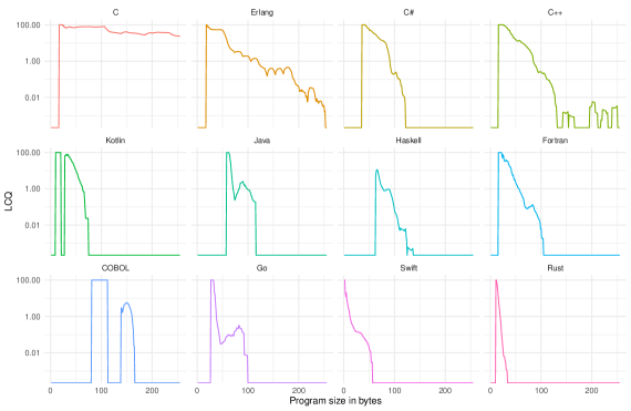
(b)

Figure 3. (a) Compilation quotients (CQs), and (b) average LCQ curves for the selected programming languages.

Fig 3(a) presents the CQ of each programming language. We observe that the CQ values are spread over a large range, with the majority of languages having a CQ below one. Only three languages are an exception to this: C, Erlang, and C++. The language with the lowest CQ is Rust at 0.0004. Strikingly, all object-oriented languages, i.e., C# (1.69), Java (0.27), C++ (0.60), and Kotlin (0.31) list in the upper half of the ranking. Moreover, newer languages such as Go (0.03), Swift (0.02) and Rust (0.00) are listed at the bottom of the ranking. There are also languages commonly considered to be similar which exhibit quite different CQ scores. For instance, C#’s CQ is over five times that of Java, and C’s CQ is over 80 times that of C++. To better understand the composition of the CQ of each measured language, we now analyze their LCQ values. Fig. 3(b) shows the LCQ as a function of size for each programming language. For almost every language, LCQ starts high i.e., near 100, and then declines to zero with some slope. A simple intuition explains this pattern: the longer the generated program, the more likely it is to contain an error. An exception to this rule is C. Its LCQ, despite initially trending downwards, does not reach zero. Instead, it stabilizes at a positive value. This behavior continues beyond 256 bytes and at least up to 1000 bytes, as shown in Fig. 4. Concretely, below 50 bytes, C’s LCQ is above 70. Between 50 and 90 bytes, it decreases sharply to around 25, followed by a sharp rise, and another sharp fall. Subsequently, it varies between 25 and 50, without exhibiting an overall increasing or decreasing trend. This suggests that C’s LCQ either never drops to zero, or does so only orders of magnitude slower than all other languages.

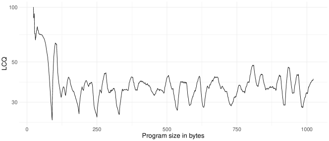
Figure 4. LCQ curve of C for a size up to 1000 bytes

Erlang lists second in the CQ ranking. Its LCQ curve behaves similarly to C’s, however with important differences. Just like C’s LCQ, it starts with a sharp drop, but then rebounds and starts to oscillate. However, unlike in C’s case, the drops are much sharper (i.e., the drop from around 50 to around 3 between 50 and 75 bytes), and the LCQ shows a clear negative trend as the size increases, reaching zero at approximately 253 bytes. C and Erlang’s oscillatory behavior already demonstrated that LCQ can be non-monotonic. These oscillations are unique to C and Erlang, but non-decreasing LCQ is not – many other tested languages exhibit non-decreasing regions e.g., Java, Fortran, and Go. COBOL’s LCQ curve also contains a significant non-decreasing region, yet it differs from the other languages in that it is caused by a lack of programs in the search space, as described below. After initially hitting zero, the LCQ curve of most languages permanently remains there. C++’s LCQ is an outlier: after an initial drop to zero, it returns to a positive value and then again drops to zero. This pattern is repeated multiple times, with the LCQ hovering on the order of $10^{-3}$. This suggests that, in the relevant region, the true LCQ hovers close to the limit of what we can measure, leading to the apparent sudden jumps on the LCQ plot. COBOL’s LCQ plot contains a region of zeroes between sizes of 113 and 138 bytes. Unlike for C++, this is not caused by all programs in the region being rejected, instead, there were no programs generated in this region. This is caused by COBOL’s verbosity. Compared to other languages, COBOL’s keywords are longer, leading to a less uniform distribution of program sizes. Because of their similarity, we also briefly describe the differences in LCQ curves of C# and Java. Despite the difference in their CQ, their LCQ curves have a similar structure. Both of them start from a near-100 value, drop sharply, briefly stabilize, and then collapse to zero. However, Java’s LCQ drops quicker than C#’s, leading to lower CQ.

4. Analysis

In this section, we interpret the results from Section 3. We first analyze the two extremes, C and Rust, and then move on to the remaining languages, comparing the behavior of related languages throughout, and finally explain CQ-affecting features.

4.1. C and Rust – the extremes

As we observed, not only is C’s CQ much higher than that of all other languages, but its LCQ curve is also peculiar: unlike all other languages, it does not approach zero. On the other extreme, we have Rust, for which only 6 out of 1.5 million programs compile. We begin our analysis with C (see Fig. 5). To better understand C’s behavior, we first look at programs below 50 bytes consisting of only one or two statements. Our first example (Fig 5(a)) shows a valid program with a declaration of a short pointer var1, and the second is an invalid program with a single continue statement appearing outside of a loop (Fig. 5(b)). The third one is an invalid program (Fig. 5(c)) with a goto statement to label var1. Since var1 is undeclared, the program is invalid. Another, more complex example is depicted in Fig. 5(d). The program defines an integer pointer with the _Thread_local modifier, which indicates there will be a separate version of the pointer for each thread main spawns. However, the program is invalid since _Thread_local variables must be either static or extern. Looking at larger programs, we observe that declarations dominate C programs, outnumbering all other types of statements. One reason for this is that C’s declarations are flexible, consist of many optional elements (specifiers), and can be arbitrarily nested. Figs. 5(e)-5(h) demonstrate this. Fig. 5(e) presents a valid declaration, nesting several pointer declarations. Fig. 5(f) likewise presents a valid program, which declares a typedef instead of a variable. Fig. 5(g) presents an invalid program which is invalid due to incorrect use of the restrict keyword which is not allowed to be applied directly to a non-pointer type (in this case, unsigned). The example in Fig. 5(h) is invalid because var2 is not a type. Fig. 6 illustrates a deeply nested but valid pointer declaration.

⬇

1

2/* valid */

3int main(void) {

4register short *var1;

5}

(a)

⬇

1

2/* invalid */

3int main(void) {

4continue;

5}

(b)

⬇

1

2/* invalid */

3int main(void) {

4goto var1;

5}

(c)

⬇

1

2/* invalid */

3int main(void) {

4_Thread_local restrict int *var2;

5}

(d)

⬇

1

2/* valid */

3int main(void) {

4extern const _Atomic long *const _Atomic *volatile _Atomic *const volatile _Atomic *const restrict volatile var1;

5}

(e)

⬇

1

2/* valid */

3int main(void) {

4typedef const volatile unsigned *const restrict volatile _Atomic *const volatile _Atomic *restrict _Atomic *volatile _Atomic var1;

5}

(f)

⬇

1

2/* invalid */

3int main(void) {

4static restrict volatile _Atomic unsigned **restrict volatile _Atomic *volatile *const restrict volatile var1;

5}

(g)

⬇

1

2/* invalid */

3int main(void) {

4extern volatile _Atomic var2 *const restrict *restrict volatile *volatile _Atomic *const volatile _Atomic var1;

5}

(h)

Figure 5. Assorted C programs generated by cq-test.

⬇

1

2/* valid */

3int main(void) {

4extern volatile _Complex *const volatile _Atomic *const restrict volatile _Atomic *const *const volatile _Atomic *const restrict *const restrict _Atomic *restrict volatile _Atomic *const restrict volatile _Atomic *volatile *const restrict _Atomic *const volatile _Atomic *const restrict _Atomic *const restrict _Atomic *const restrict _Atomic *const _Atomic(*volatile _Atomic *const *volatile _Atomic **const _Atomic *_Atomic *const restrict *const restrict volatile _Atomic *const restrict *restrict volatile **const restrict volatile _Atomic *restrict volatile _Atomic *const restrict volatile _Atomic *restrict _Atomic *const **restrict volatile _Atomic *const restrict *volatile *_Atomic *const restrict _Atomic *const *const volatile(*const restrict var2));

5}

Figure 6. A 780-byte long, valid C program.

Another key aspect of C’s declarations is that they impose few conditions. Particularly for pointer declarations, which dominate longer programs, the number of conditions does not increase as they are nested. To understand this, let us contrast this with nested arithmetic expressions for which the constraints do increase. Consider an expression a + b. It is valid if (1) a and b are individually valid, and (2) a and b have types that can be added together. Condition (2) is imposed on the subexpressions by its parent. If these subexpressions are themselves composed of other expressions, they may have to impose additional conditions on their subexpressions to satisfy condition (2). Hence the number of conditions may grow as the expression becomes longer, making it harder to generate valid nested expressions. By contrast, in a C pointer declaration T *D, no conditions are imposed on declarator D. Hence, compiling nested pointer declarations does not become harder as declarations get longer.

To examine whether this behavior leads indeed to C’s higher LCQ, we calculated the LCQ of two variants of C: one without pointer declarations, and one without any declarations. Fig. 7 presents the LCQ of these variants up to 1000 bytes. Without any declarations, C’s LCQ falls quickly to zero. The variant without pointer declarations (but with all other types of declarations) exhibits a significantly higher LCQ, but it also plummets to zero at around 950 bytes. This shows that pointer declarations are essential for C’s LCQ not to plummet.

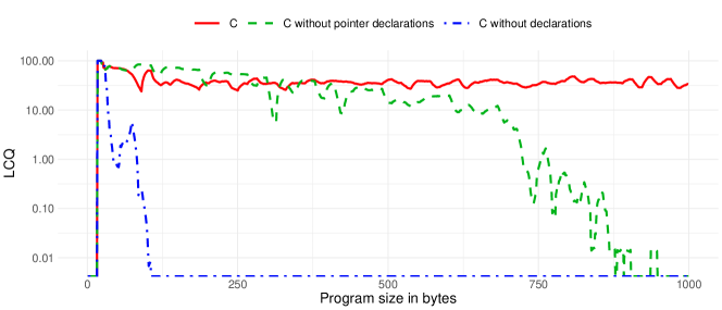
Figure 7. LCQ curve of C, C without pointer declarations, and C without declarations, up to 1000 bytes

In many ways, Rust behaves differently from C. The generated Rust programs are dominated by operator expressions, which, as explained above, are less likely valid under increasing length. Furthermore, Rust’s type system is strict; it does not accept operands of mismatching types. For example, 1u32 + 2u8 and 1u32 + (’a’ == ’a’) is invalid Rust, but valid C. This means that, while most of the programs are operator expressions, the probability that such expressions compile is extremely small. This in turn leads to very low CQ. In essence, both C and Rust have a construction that dominates as program size increases, but C’s programs are likely valid, while Rust’s programs become unlikely to be valid with growing size.

Fig. 8 presents Rust examples. Rust’s type system permits some constructions that would not be valid in most other imperative languages. For example, Fig. 8(a) shows a valid program that negates the result of a return expression. return has type ! (never/bottom), which implements the Not trait, overloading the negation operator. Thus !return has type !, which is coercible to (). main’s return type is (), thus the program is valid. Fig. 8(b) presents a similar example. return as _ casts return to an inferred type. This type is inferred to be (), as that main’s return type. Since ! is castable to any type, the program is valid. The majority of Rust samples, however, are invalid. Fig. 8(c) shows an invalid operator expression, adding a 32-bit integer to a 16-bit one. Fig. 8(d) presents a longer example, which divides a string by an integer and assigns to a temporary value, and is thus invalid.

⬇

1

2// valid

3fn main() {

4!return

5}

(a)

⬇

1

2// valid

3fn main() {

4return as _

5}

(b)

⬇

1

2// invalid

3fn main() {

442u32 + 42u16

5}

(c)

⬇

1

2// invalid

3fn main() {

4"string" / 42isize >= 42i128 ^= 123.4f32 /= 42u16

5}

(d)

Figure 8. Assorted Rust programs found by cq-test.

4.2. Comparison of related languages

This section compares the behavior of related languages such as C and C++, Java and C#, C++ and C#. Fortran, COBOL, Go and Swift are treated in Section 4.3.

C and C++

C++ is almost a superset of C. Hence, it is striking that C++’s CQ is so much smaller than that of C. Furthermore, C++ also has the pointer declarations causing C’s non-collapsing LCQ curve. It is thus natural to ask: Why does C++’s LCQ curve plummet to zero while C’s curve does not? As our results reveal, the answer is that C++ has other features that dominate pointer declarations, but are unlikely to be valid. These features include namespace definitions and using declarations. Furthermore, within these constructions, other flexible, but hard to compile features are nested: qualified identifiers, e.g., var2::var1::var1::var2::var1, templates, and operator function identifiers, e.g., operator + occur frequently. Programs including these features are less likely to compile than C’s pointer declarations. In particular, qualified identifiers are highly unlikely to compile, as doing so requires multiple matching namespace declarations. Fig. 9(a) presents an example which first declares a label var1, then uses a using-declaration bringing ::operator new[] into the current scope (this is essentially a no-op, as the operator is already in the global scope). It then also declares an empty enum class. Fig. 9(b) also depicts a valid program containing three using-declarations, the first one with a label. Fig. 9(c) presents an example with a generic operator, with the generic parameter itself being an operator nested within several namespaces. Neither the referenced namespaces nor the operators exist, thus the program is invalid. Fig. 9(d) presents a declaration that uses many modifiers, and is invalid due to the use of the friend modifier outside a class. Despite the complications with matching namespaces etc., C++ still has a high CQ compared to other languages, as smaller programs do compile frequently. These programs contain empty blocks ({}), simple declarations, etc. similar to C.

⬇

1

2// valid

3int main() {

4var1: using ::operator new[];

5enum class var1;

6}

(a)

⬇

1

2// valid

3int main() {

4var2: var1: using ::operator delete[];

5using ::operator delete;

6using ::operator delete[];

7}

(b)

⬇

1

2// invalid

3int main() {

4using ::operator!<::var1::var2<>::var1::var1::var2::template operator^=...>;

5}

(c)

⬇

1

2// invalid

3int main() {

4friend register static thread_local extern mutable inline virtual explicit typename var1::var2::template var2<>;

5}

(d)

Figure 9. Assorted C++ programs found by cq-test.

C# and Java

C# and Java are both popular object-oriented languages, with many similarities. Despite this, C# has higher CQ than Java, but their LCQ curve is quite similar. C#’s higher CQ can be explained by its LCQ curve decreasing less rapidly. One factor contributing to this smaller slope is that C#’s entry point is shorter than Java’s. This does not necessarily imply a higher CQ, but C#’s small programs are also likely to compile, whereas in Java’s case, we can observe an early drop in LCQ. Fig. 10 and 11 present C# and Java programs respectively. At smaller sizes, C# programs consist of many declarations, similar to C and C++. In particular, multi-dimensional array declarations, such as in Fig 10(a), are common. By contrast, Java programs consist of expressions or control-flow statements that contain expressions, as seen in Fig. 11(a). Although Java’s type system is lax for expressions e.g. permitting ’a’ == 123.4d, many expressions are still invalid due to type errors. Consider, e.g., Fig. 11(b), an invalid program with an if-statement that has a double in its condition. This trend extends to larger programs with longer expressions which are more likely to contain errors. An example is shown in Fig. 11(d), which contains an invalid use of the increment operator, and several instances of incorrect operand types. A longer valid Java program is depicted in Fig. 11(c), with correct usage of expressions and looping. In C#’s case, longer programs are dominated by generic local function declarations instead of expressions. These can be made arbitrarily long by adding more generic constraints, which are unlikely to compile. Fig. 10(b) and 10(c) present a valid and invalid example of generic local functions respectively. Fig 10(b) shows a valid C# program declaring a local function var1, with a generic parameter also named var1, which is bound by two constraints: var1: class?, whic prescribes that it must be a (potentially nullable) reference type, and var1: var1, which prescribes that it must be var1 or a subclass of var1. Fig. 10(c) declares a local function, but it attempts to constrain nonexistent generic parameters, and thus is invalid. The latter type of programs is much more common than the former, hence C#’s LCQ plummets to zero at large program sizes.

⬇

1

2// valid

3void Main() {

4ulong [,,,,] var2;

5}

(a)

⬇

1

2// valid

3void Main() {

4void var1<var1>() where var1 : class?, new() {}

5}

(b)

⬇

1

2// invalid

3void Main() {

4void var1() where var2 : new() where var1 : class?, var1 {}

5}

(c)

Figure 10. Assorted C# programs found by cq-test. The class enclosing the Main functions is omitted for brevity.

⬇

1

2// valid

3void main(String[] args) {

4assert ’a’ == 123.4d;

5}

(a)

⬇

1

2// invalid

3void main(String[] args) {

4if(123.4)

5throw true;

6}

(b)

⬇

1

2// valid

3void main(String[] args) {

4while(-’a’ <= + 123.4d + ’a’) var2:

5continue;

6}

(c)

⬇

1

2// invalid

3void main(String[] args) {

4assert ++123.4d }

(d)

Figure 11. Assorted Java programs found by cq-test. The class enclosing the main functions is omitted for brevity.

⬇

1

2// valid

3fun main() {

4open class var1 <out var1>

5}

(a)

⬇

1

2// invalid

3fun main() {

4interface var2

5}

(b)

⬇

1

2// valid

3fun main() {

4var1@ var2@ var2@ var1@ class var2

5}

(c)

⬇

1

2// invalid

3fun main() {

4open inner internal abstract class var2<in *, out var1,> override operator infix inline suspend abstract final constructor(var var2: dynamic)

5}

(d)

Figure 12. Assorted Kotlin programs generated by cq-test.

C# and C++

C# and C++ are close in the CQ ranking. Indeed, C#’s CQ is closer to C++’s than Java’s. This is because both languages are prone to generating declarations instead of expressions. Declarations are more likely to compile, as they have few conditions imposed on them. Interestingly, while C++ programs often contain qualified identifiers, these are seldom generated in C#.

Kotlin and Java

Kotlin combines object-oriented paradigms with functional ones and compiles to JVM. Compared to Java, it has a slightly higher CQ. While Java’s programs are dominated by expressions, Kotlin’s programs are instead dominated by declarations. This is explained by the fact that Kotlin has many more types of declarations and modifiers than Java, giving the generator more options. Fig. 12(a) presents a simple valid declaration, while Fig. 12(b) presents a simple declaration that is invalid, as interfaces cannot be defined locally within a function. Fig. 12(d) is an example of a long, invalid declaration. The program attempts to define a local generic class with a constructor. However, it has many errors, including the usage of modifiers that are not applicable, incorrect use of star projections, and incorrect use of dynamic types. A feature that increases Kotlin’s CQ, however, is that multiple labels are allowed to have the same name, unlike in Java. Fig. 12(c) presents an example that reuses two label names on a declaration. Overall, because of its richer declarations, Kotlin behaves more similarly to C or C# than Java. However, Kotlin’s declarations are less likely to compile than those of languages with higher CQs.

⬇

1

2func() -> + + + + - 42.

(a)

⬇

1

2func() -> catch catch not not not bnot fun an_atom:an_atom/42.

(b)

⬇

1

2func() -> + + + - + - - Var2.

(c)

⬇

1

2func() -> catch bnot + fun an_atom:an_atom/42:"string" "string".

(d)

Figure 13. Assorted Erlang programs generated by cq-test.

⬇

1

2-- valid

3func = func

4where { func = -func; }

(a)

⬇

1

2-- invalid

3func = 42

4where { var1 = -’a’; }

(b)

⬇

1

2-- valid

3func = var2

4where { var2 = (#,#) (,,,,,) {}; }

(c)

⬇

1

2-- invalid

3func = 42

4where { var2 = mdo {} @ ’var1; }

(d)

⬇

1

2-- invalid

3func = var2

4where { func = func :: forall. forall -> var2 :: - ’‘func‘ + ‘func‘ : + ‘var1‘ + : ’‘func‘ ’‘func‘ - ‘var1‘ ’ + -; }

(e)

Figure 14. Assorted Haskell programs generated by cq-test.

Erlang and Haskell

Erlang and Haskell are purely functional languages. Their CQs are very different, with Erlang having the second highest CQ among tested languages, and Haskell having the sixth lowest. Erlang’s high CQ is mostly a result of its dynamic typing, because of which even clearly type-incorrect programs are deemed valid (but will raise type errors on execution). Erlang programs necessarily consist only of expressions, as nothing else is permitted inside a function. As a result, Erlang exhibits an initially high LCQ, which falls slowly. Fig. 13(a) presents a valid program which defines a function returning -42. The multiple plus operators have no effect. Fig. 13(b) presents a program that is deemed valid but will crash at runtime because of type errors. It also creates an anonymous function that calls the function an_atom:an_atom with arity 42. This function does not exist, which is another reason why the program fails at runtime. Fig. 13(c) shows an example similar to Fig. 13(a), except it is invalid due to its use of an undeclared identifier. Fig. 13(d) depicts another, more elaborate invalid program. The code attempts to perform a function call of the form <Module>:<Function>. However, it specifies a function instead of a module name and a string instead of a function identifier. This is syntactically valid as Module and Function can arbitrary expressions. Furthermore, the expression "string" "string" is valid and equivalent to "stringstring".

Different from Erlang, Haskell is statically typed. Haskell’s LCQ steeply decreases as more and more programs encounter type errors. However, recursion and Haskell’s flexible type system allow some programs to compile, leading to a higher CQ than other languages. Fig. 14(a) presents a Haskell program which recurses to make func a value of type Num a => a. The program is valid but does not terminate. Fig. 14(b) depicts a program which is invalid because of a type error, as it attempts to negate the character ’a’. Fig. 14(d) is a more complicated invalid program: it contains an empty mdo block, and a template Haskell quotation of var1, which is undefined. Tuples are also often used in longer Haskell programs. Fig. 14(c) presents a valid program combining several elements – (,,,,,) {} performs a ”construction using field labels” (mar, 2010, Section 3.15.2) of a 6-tuple without specifying any field labels, resulting in a tuple of type (a,b,c,d,e,f). This tuple is then applied to the unboxed binary tuple constructor (#,#), resulting in a type of g -> (# (a,b,c,d,e,f), g #). The function would raise an error on execution, as the constructor (,,,,,) is not a record constructor, and therefore the elements of the tuple are not properly initialized. Finally, programs with Template Haskell quotes, backticks, and type applications are rejected by GHC (see Fig. 14(e)).

4.3. Analysis of Fortran, Cobol, Go and Swift

We consolidate Fortran, COBOL, Go and Swift. Fortran programs are dominated by type declarations, which have many features and parameters, and thus seldom compile. Fig. 15(a) is a valid example, declaring a multidimensional character array, while Fig. 15(b) presents an example that is invalid because it uses a complex literal and a string as an array length. COBOL’s CQ is extremely close to that of Fortran, and its behavior is also similar, with declarations dominating. In particular, RENAMES clauses are common, and are prone to errors due to undeclared identifiers and other semantic errors (e.g. Fig. 15(d)). Fig. 15(c) presents a valid program that declares a national data item.

⬇

1

2! Fortran, valid

3PROGRAM MAIN

4TYPE var1

5CHARACTER (LEN = *), POINTER :: var1(:) * 42

6ENDTYPE

7END

(a)

⬇

1

2! Fortran, invalid

3PROGRAM MAIN

4TYPE var1

5CHARACTER * (-42, -42) :: var1(:) * ’string’

6ENDTYPE

7END

(b)

⬇

1

2* COBOL, valid

3DATA DIVISION.

4WORKING-STORAGE SECTION.

577 var2 PICTURE N.

6PROCEDURE DIVISION.

7END PROGRAM test.

(c)

⬇

1

2* COBOL, invalid

3DATA DIVISION.

4WORKING-STORAGE SECTION.

566 var1 RENAMES var1 OF var1 THROUGH var1 OF var2.

666 var2 RENAMES 42 IN 42 THROUGH 42 OF var2.

7PROCEDURE DIVISION.

8END PROGRAM test.

(d)

⬇

1

2// Go, invalid

3func main() {

4go + & & var1.var2.var1 &^ <- & + * - <- ^ * ! + ! ^ & <- var1.var2.var1 && * ! + - - <- * ^ ^ * nil.var1 >> & "string".var2

5}

(e)

⬇

1

2// Swift, valid

3do {} catch {};

(f)

⬇

1

2// Swift, invalid

3try var1(var2:).

4init.init($1:).

5init($0:).

6init($0:).init(var2:);

(g)

⬇

1

2// Go, valid

3func main() {

4goto var1

5var1:

6select {}

7goto var1

8}

(h)

Figure 15. Assorted Fortran, COBOL, Go, and Swift programs generated by cq-test.

Unlike the other two languages, Go is dominated by expressions and some control-flow structures. Srict typing and features that require a particular type of expression lead to a low CQ. Fig. 15(h) presents a valid program which correctly uses goto statements. Fig. 15(e) presents an expression that is invalid because (among other errors) the argument of its go statement is not a function call. Finally, Swift achieves the second-lowest CQ of all languages due to frequent use of initializer prefixes, as well as the use of implicit parameter names (e.g. $0) outside closures. Fig. 15(f) is a simple valid example, while Fig. 15(g) is an invalid example that demonstrates the issues mentioned above.

4.4. Analysis of CQ-affecting language features

A common observation in high-CQ languages are (1) flexible features, i.e. features that can grow arbitrarily, and (2) easy-to-compile features, i.e. a random instance of the given feature is likely accepted by the compiler. In C’s case, these are pointer declarations, in Erlang’s case these are expressions. Conversely, low-CQ languages have features that are flexible, but hard to compile. For Rust and Swift, these are expressions. The languages with less extreme CQs have mixes of different features. For instance, a language can start with easy-to-compile features at small sizes, but at higher sizes new structures become available that are more flexible and harder to compile (e.g. C#). The two most influential features for CQ are expressions and declarations. Expressions are flexible since they can be nested in all languages e.g. operator expressions and function calls. Their compilation hardness is determined by the strictness of the type system. Declarations, on the other hand, vary in their flexibility. Their compilation hardness is usually not caused by the type system. Other common features, such as control-flow statements are less frequent.

Languages with more complex features usually also allow more complex declarations. This leads to more restrictions, thus lower CQ. Another important aspect is whether declarations are allowed inside functions. For example, Rust has no shortage of complex features (e.g., traits), yet they cannot be declared within functions. Thus, they also do not affect the CQ of the language. Other languages, such as Swift, permit a high variety of declarations within functions, increasing the importance of declarations to CQ. In a nutshell, highly general constructs cause lower CQ. On the other hand, the strictness of the type system is secondary, mostly influencing how difficult expressions are to compile. For C, the modest complexity of constructs leads to easy-to-compile declarations, while for Erlang, the lack of static typing leads to easy-to-compile expressions, both leading to high CQ.

5. Discussion

Having analyzed CQ values and LCQ graphs of programming languages, we discuss CQ’s implications on (1) programmers, (2) the long-run adoption of programming languages, and, (3) the fuzz-testing of compilers. Finally, we discuss the limitations of our work.

CQ and non-novice programmers

CQ measures the difficulty of writing valid programs in programming language $\mathit{PL}$ without knowing anything other than $\mathit{PL}$’s syntax. As analyzed in the previous section, the CQ of a language $\mathit{PL}$ is affected by the semantic complexity and flexibility of $\mathit{PL}$’s features, and their prevalence in the program space. Put differently, CQ is influenced by how hard it is for a randomly generated program to use a given feature correctly. We argue that there is a connection between CQ and the semantic complexity experienced by non-novice programmers.

A programmer’s task is to write programs that compile. For the programmer, this implies producing programs that are both syntactically and semantically valid. While syntax is mostly a barrier for novices, we argue that CQ measures a part of the semantic complexity experienced by non-novice programmers. Intuitively, if frequently-used features, such as variable declarations, are likely to compile when generated randomly, then it also takes low effort for the programmer to get them right. The programmer can then concentrate on other things instead. Conversely, if frequently-used features are unlikely to compile at random, this indicates higher effort for the programmer. CQ can help language designers evaluate a feature’s effects before its release.

Long-run adoption of programming languages

Firstly, it is striking that the four most popular languages of the TIOBE index are all placed in the top half of the CQ ranking. This could suggest that languages with high CQ are more likely to become and remain popular. Secondly, newer languages have lower CQs than older languages. This could be explained by the recent trend towards feature-rich and type-safe programming languages, increasing language complexity but decreasing CQ. Particularly, Rust with a CQ of almost zero, is known for having a steep learning curve with a significant proportion of learners abandoning it because of its difficulty (Group, 2023).

Implications on compiler testing

Another striking finding is C’s much higher CQ compared to all other languages. We argue that this could partially explain the success of testing campaigns for C compilers  (Yang et al., 2011; Le et al., 2014). Since C compilers have higher CQ i.e., are more permissive, they are also more accessible for testers. Conversely, compilers of low CQ languages such as Haskell and Rust are more difficult to test. This is especially plausible since many testing approaches for compilers implement the language grammars programmatically. As CQ can be a proxy for the effectiveness of fuzzers for a given language, language designers can use cq-test to optimize for high CQ.

Limitations

Our tool cq-test enables a large-scale study of the CQs of 12 popular compiled programming languages. However, we acknowledge that our work also comes with limitations. CQ is defined using the proportion of compiling programs to the total number of syntactically valid programs. One limitation of our work is that we measured CQ only on programs with a single entry point and forbade use of the language’s standard library. However, this ignores other important features contributing to a language’s complexity such as includes in C/C++ and traits in Rust. Moreover, CQ does not consider the complexity of the language’s runtime semantics.

6. Related Work

We survey three strands of related work on (1) automated program generation, (2) property-based testing, and (3) empirical studies on programming language learning.

Automated program generation

The earliest work laying the ground for automated program generation is Lisp’s meta-programming, manipulating source code as a data structure by John McCarthy. Approaches in program synthesis are also related to our approach because these also use program enumeration, e.g., FlashFill (Gulwani, 2011). However, their goals are different. Synthesis aims to find a program satisfying a specification. Our approach generates programs to compute CQs. Genetic programming (Koza, 1992) is another approach for program generation from progressively unfit-to-fit programs using selection, crossover, replication, and mutation strategies on the program’s ASTs. Another closely related line of research is Grygiel and Lescanne [(2013)]’s work on counting terms of the lambda calculus, combinatorial properties, and asymptotic distribution on random generation. They observe that lambda calculus’s CQ converges to zero. Similarly, in our work, all languages show this behaviour. The only exception is C for which even many sizeable programs compile.

Property-based testers and grammar-based fuzzers

Our work is based on the exhaustive enumerator FEAT (Duregard et al., 2012), which belongs to the family of property-based testers such as LeanCheck by Rudy Matela, SmallCheck (Runciman et al., 2008), and QuickCheck (Claessen and Hughes, 2000). Different from property-based testers whose test drivers are usually manually written, our approach generates test drivers from a context-free grammar automatically. Grammar-based black-box fuzzers (Burkhardt, 1967; Hanford, 1970; Yang et al., 2011) are all also technically related to our approach. However, our work and fuzzers differ in their objective. The objective of a fuzzer is to find bugs, while we aim to measure the compilation quotient.

Empirical studies on programming languages

Our study is related to studies on programming languages. Ray et al. [(2014)] study how programming languages affect software quality from large datasets based on GitHub users while other work studies key factors in adopting programming languages with user surveys (Meyerovich and Rabkin, 2013). More loosely related is work on how people learn computer programming (Guo, 2013) and studies that compare the cognitive load of Python programming against programming in a visual programming language such as Algot (Thorgeirsson et al., 2024).

7. Conclusion and Future Work

We introduced the compilation quotient (CQ), a metric for the compilation hardness of compiled programming languages. The key idea is measuring the CQs of programming languages by sampling programs from context-free grammars using a bucket-based sampling algorithm. With our framework cq-test, we computed the CQs of twelve popular compiled programming languages. Our findings show high variation: the language with the highest CQ is C with a CQ of almost 50 leading by a large margin over all other languages. Strikingly, Rust’s CQ is almost zero. For all languages, the number of observed compiling programs drops to zero within the measured size range, but C is an exception, showing a high number of compiling programs even at large sizes. Long programs are dominated by either declarations or expressions – CQ is then significantly affected by how much the language restricts these constructs. CQ is related to extrinsic properties of programming languages – the most popular languages have a high CQ (e.g., C++, Java, C#), while newer languages have lower CQs (e.g. Rust). We believe that CQ is a useful metric for the comparison and analysis of programming languages, providing valuable information to designers of future languages. By providing a framework for more objective discussions of language complexity, CQ can help programmers to make more informed decisions.

We outline three avenues of future work. First, we aim to extend CQ to interpreted languages. Unlike in compiled languages where ahead-of-time compilers reject invalid programs with errors, interpreters’ errors could be either caused by invalidity (e.g. type errors, incorrect declarations, etc.) or runtime issues (e.g. division by zero, null reference, etc.). Hence, a key challenge in extending the CQ to interpreted languages is to categorize interpreter errors. Another direction of future work is to generate more complex programs e.g., with more than a single function. Supporting the sampling of complex programs requires that the sampled program declare identifiers before their first use. Otherwise, the chances of generating valid programs are very small. Finally, it might be worthwhile to investigate how difficult it is to fix errors in different programming languages. One possible way to do this is to present each rejected program to a large language model, ask the model to fix the error, and then check whether the fixed program compiles.

References

- (1)
- for (1991) 1991. Information technology — Programming languages — Fortran — Part 1: Base language. Fortran 90 standard.
- mar (2010) Simon Marlow (Ed.). 2010. Haskell 2010 language report. https://www.haskell.org/onlinereport/haskell2010/
- ANSI X3J4 Committee (1985) ANSI X3J4 Committee. 1985. COBOL 85 Standard. Technical Report. American National Standards Institute, New York, NY, USA. ANSI X3.23-1985.
- Authors (2023) The Go Authors. 2023. Go 1.20 Release Notes. https://tip.golang.org/doc/go1.20
- Burkhardt (1967) W.H. Burkhardt. 1967. Generating test programs from syntax. In Computing. 53–73.
- Claessen and Hughes (2000) Koen Claessen and John Hughes. 2000. QuickCheck: A Lightweight Tool for Random Testing of Haskell Programs (ICFP ’00). New York, NY, USA, 268–279.
- Duregard et al. (2012) Jonas Duregard, Patrick Jansson, and Meng Wang. 2012. FEAT: Functional Enumeration of Algebraic Types. In Haskell ’12. 61–72.
- Gosling et al. (2021) James Gosling, Bill Joy, Guy Steele, Gilad Bracha, and Alex Buckley. 2021. The Java Language Specification, Java SE 17 Edition. https://docs.oracle.com/javase/specs/jls/se17/html/index.html
- Group (2023) Rust Survey Working Group. 2023. 2022 Annual Rust Survey Results. https://blog.rust-lang.org/2023/08/07/Rust-Survey-2023-Results.html
- Grygiel and Lescanne (2013) Katarzyna Grygiel and Pierre Lescanne. 2013. Counting and generating lambda terms. Journal of Functional Programming 23, 5 (2013), 594–628. https://doi.org/10.1017/S0956796813000178
- Gulwani (2011) Sumit Gulwani. 2011. Automating string processing in spreadsheets using input-output examples. In POPL. ACM, 317–330.
- Guo (2013) Philip J. Guo. 2013. Online Python Tutor: Embeddable Web-Based Program Visualization for CS Education. In Proceedings of the 44th ACM Technical Symposium on Computer Science Education. ACM, 579–584.
- Hanford (1970) K. V. Hanford. 1970. Automatic generation of test cases. IBM Systems Journal 9, 4 (1970), 242–257.
- Inc. (2021) Apple Inc. 2021. Swift 5.4 Release Notes. https://www.swift.org/blog/swift-5.4-released/
- International Organization for Standardization (2014) International Organization for Standardization. 2014. ISO/IEC 14882:2014: Information technology — Programming languages — C++. Technical Report. Standard.
- ISO/IEC (2011) ISO/IEC. 2011. ISO/IEC 9899:2011 - Information technology – Programming languages – C. Standard ISO/IEC 9899:2011. International Organization for Standardization, Geneva, Switzerland.
- JetBrains (2023) JetBrains. 2023. Kotlin 1.4 Release Notes. https://kotlinlang.org/docs/whatsnew14.html
- Koza (1992) John R. Koza. 1992. Genetic Programming: On the Programming of Computers by Means of Natural Selection. MIT Press, Cambridge, MA, USA.
- Le et al. (2014) Vu Le, Mehrdad Afshari, and Zhendong Su. 2014. Compiler validation via equivalence modulo inputs. In PLDI. 216–226.
- Marlow (2009) Simon Marlow. 2009. [Haskell] Announcing Haskell 2010. https://mail.haskell.org/pipermail/haskell/2009-November/021750.html
- Meyerovich and Rabkin (2013) Leo A. Meyerovich and Ariel S. Rabkin. 2013. Empirical Analysis of Programming Language Adoption. In OOPSLA (OOPSLA ’13). Association for Computing Machinery, 1–18.
- Microsoft (2015) Microsoft. 2015. What’s New in C# 6. https://docs.microsoft.com/en-us/dotnet/csharp/whats-new/csharp-6
- Parr et al. (2014) Terence Parr, Sam Harwell, and Kathleen Fisher. 2014. Adaptive LL(*) Parsing: The Power of Dynamic Analysis. In OOPSLA ’14. 579–598.
- Ray et al. (2014) Baishakhi Ray, Daryl Posnett, Vladimir Filkov, and Premkumar Devanbu. 2014. A Large Scale Study of Programming Languages and Code Quality in Github. In FSE ’14. 155–165.
- Runciman et al. (2008) Colin Runciman, Matthew Naylor, and Fredrik Lindblad. 2008. Smallcheck and Lazy Smallcheck: Automatic Exhaustive Testing for Small Values. In Haskell ’08. 37–48.
- Team (2021) The OTP Team. 2021. OTP 23.3. https://www.erlang.org/patches/otp-23.3
- Team (2022) The Rust Language Team. 2022. Announcing Rust 1.60.0. https://blog.rust-lang.org/2022/04/07/Rust-1.60.0.html
- Thorgeirsson et al. (2024) Sverrir Thorgeirsson, Theo Weidmann, Karl-Heinz Weidmann, and Zhendong Su. 2024. Comparing Cognitive Load Among Undergraduate Students Programming in Python and the Visual Language Algot. In SIGCSE ’24 (to appear). ACM.
- Yang et al. (2011) Xuejun Yang, Yang Chen, Eric Eide, and John Regehr. 2011. Finding and Understanding Bugs in C Compilers. In PLDI ’11. 283–294.