TDT Loss Takes It All:
Integrating Temporal Dependencies among Targets
into Non-Autoregressive Time Series Forecasting

Abstract

Learning temporal dependencies among targets (TDT) benefits better time series forecasting, where targets refer to the predicted sequence. Although autoregressive methods model TDT recursively, they suffer from inefficient inference and error accumulation. We argue that integrating TDT learning into non-autoregressive methods is essential for pursuing effective and efficient time series forecasting. In this study, we introduce the differencing approach to represent TDT and propose a parameter-free and plug-and-play solution through an optimization objective, namely TDT Loss. It leverages the proportion of inconsistent signs between predicted and ground truth TDT as an adaptive weight, dynamically balancing target prediction and fine-grained TDT fitting. Importantly, TDT Loss incurs negligible additional cost, with only $\mathcal{O}(n)$ increased computation and $\mathcal{O}(1)$ memory requirements, while significantly enhancing the predictive performance of non-autoregressive models. To assess the effectiveness of TDT loss, we conduct extensive experiments on 7 widely used datasets. The experimental results of plugging TDT loss into 6 state-of-the-art methods show that out of the 168 experiments, 75.00% and 94.05% exhibit improvements in terms of MSE and MAE with the maximum 24.56% and 16.31%, respectively.

1 Introduction

Due to the powerful nonlinear modeling capabilities of neural networks, deep learning-based time series forecasting methods have achieved outstanding performance in many real-world applications such as finance [1], transportation [2], energy [3], and climate [4]. Within these methods, the encoder-decoder architecture is extensively utilized, wherein the encoder first maps historical time series into context vectors, and then the decoder maps them into predictions in an autoregressive (AR) or non-autoregressive (NAR) paradigm [5]. As illustrated in Figure 1, the AR methods recursively yield single-step prediction based on the previous prediction and hidden representation [6, 7, 8]. In contrast, NAR methods directly output multi-step predictions [9, 10, 11]. Specifically, AR methods consider temporal dependencies among the predicted sequence to boost modeling accuracy but suffer from error accumulation and inefficiency due to sequential inference, while NAR methods neglect these dependencies. This trade-off between effectiveness and efficiency poses a challenge. While existing studies  [12, 13, 14] have brushed over this challenge by introducing auxiliary features, e.g., positional encoding or timestamps (e.g., minutes, hours, weeks), a comprehensive exploration of learning temporal dependencies among the predicted sequence is largely insufficient. We investigate an interesting question: Could we combine the advantages of AR and NAR paradigms to make a more efficient and effective time series forecasting?

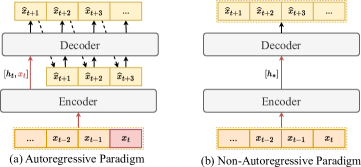
Figure 1: Illustration of two common paradigms in time series forecasting.

To answer this question, the key lies in modeling and leveraging the temporal dependencies among the predicted sequence. To facilitate the representation and learning of these dependencies, we propose to view the predicted sequence as a set of prediction targets, where each time step is considered as an individual target. For clarity, we refer to the Temporal Dependencies among Targets as TDT. In this paper, we delve into the significance of TDT in time series forecasting and propose a simple yet intuitive representation of TDT using the differencing approach to facilitate understanding and learning of TDT. To combine the strengths of both AR and NAR paradigms, we present a parameter-free, plug-and-play solution with negligible additional computational costs by introducing a novel optimization objective called TDT Loss. The TDT Loss comprises two loss components and an adaptive weight. The first loss component measures the model’s performance on target prediction, while the second quantifies the model’s performance in fitting fine-grained TDT. The adaptive weight adjust the importance of the two loss components and is determined by the model’s performance in predicting coarse-grained TDT. The TDT Loss guides the non-autoregressive time series forecasting models, which we refer to as base models, to dynamically focus on target prediction and TDT learning. Through this approach, the model progressively improves its understanding of the time series, ultimately achieving substantial performance improvements by accurately forecasting both targets and their temporal dependencies. In summary, our contributions are as follows:

• Inspired by the analysis of autoregressive and non-autoregressive paradigms, we propose to integrate the learning of TDT into non-autoregressive models. This integration allows us to leverage the strengths of both paradigms for effective and efficient time series forecasting.

• We provide a parameter-free, plug-and-play solution with negligible additional computational costs through the proposed optimization objective, TDT Loss. It can be seamlessly integrated into any non-autoregressive time series forecasting model, guiding the model to dynamically focus on target prediction and TDT learning in an end-to-end manner.

• Experimental results show that TDT Loss significantly enhances the non-autoregressive time series forecasting methods, proving the effectiveness and generality of the proposed method. Especially, out of the 168 experiments, 75% show improvements in MSE, and 94.05% exhibit improvements in MAE, with the maximum improvements reaching 24.56% and 16.31%, respectively.

2 Related Work

Autoregressive Time Series Forecasting: Traditional time series forecasting methods, such as ARIMA[15], primarily rely on statistical principles and capture trends, seasonality, and autocorrelation in time series data by establishing linear AR models. However, these linear AR methods struggle to capture complex nonlinear patterns and often perform poorly when faced with high-dimensional and long-sequence time series data[16], limiting their applicability in real-world scenarios. In recent years, the rapid development of deep learning techniques has provided new opportunities for solving time series forecasting problems. Deep AR models, such as LSTM[6], GRU[7], and DeepAR[8], have been widely adopted in time series forecasting tasks. These models sequentially predict each target by taking historical sequence data and the predicted results before each target as input, thus enabling them to model TDT. However, the recursive structure of AR models leads to slow prediction speed, as they need to generate results step by step. Moreover, the error at each prediction step may propagate and accumulate in subsequent predictions, leading to a decline in prediction quality[17, 18]. These limitations make it challenging for AR models to meet the requirements of long-sequence input and prediction in practical applications, especially in scenarios that demand real-time or near-real-time forecasting.

Non-Autoregressive Time Series Forecasting: To address the limitations of AR models and improve prediction efficiency, researchers have proposed various NAR time series forecasting models. These models include methods based on convolutional neural networks (CNNs)[11, 19, 20, 21], multilayer perceptrons (MLPs)[22, 23, 9, 24, 25], and Transformers[12, 10, 14, 26, 27]. CNNs-based NAR models utilize convolutional operations to capture local patterns and multi-scale features in time series. MICN[20] uses multiple branches with different convolutional kernels to model different latent pattern information of the sequence separately and TimesNet[21] observes that real-world time series often exhibit multi-periodicity and proposes a method to reveal the complex interactions within and between these periods. MLPs-based NAR models use a series of fully connected layers to model time series. DLinear[23] utilizes an average pooling operation to extract the trend and seasonality components of the time series and use simple linear layer to obtain the final prediction. RLinear[24] further enhances the MLP-based NAR models by introducing a reversible normalization layer between two linear layers. Transformers-based NAR models capture the global dependencies in time series through self-attention mechanisms. PatchTST[26] divides time series into multiple patches and uses Transformer to model these patches to capture local and global dependencies, while iTransformer[27] treats independent time series as tokens, captures multivariate correlations through self-attention, and utilizes layer normalization and feed-forward network modules to learn better global representations of sequences for time series forecasting.

Although these NAR models have significantly improved prediction efficiency, they often ignore TDT, which may lead to a decrease in prediction performance. Some studies incorporate positional encoding or timestamp features to reflect the temporal order of prediction targets, but these approaches only enable the model to implicitly capture the TDT [12, 13, 14]. To address these limitations, we propose a novel approach that guides NAR models to explicitly learn TDT while maintaining their inherent advantages, thereby enhancing the overall performance of time series forecasting.

3 Proposed Method

3.1 Problem Formulation

In the time series forecasting task, given a historical time series $X_{t}=\left\{x_{t-L+1},x_{t-L+2},\cdots,x_{t}\right\}\in\mathbb{R}^{L\times N}$ with $N$ variables and $L$ time steps, where each $x_{t}\in\mathbb{R}^{N}$, our objective is to learn a model $F$ with parameters $\Theta$ to predict the future sequence $\widehat{Y}_{t}=\left\{\hat{x}_{t+1},\hat{x}_{t+2},\cdots,\hat{x}_{t+H}\right\}\in\mathbb{R}^{H\times N}$ with $H$ time steps simultaneously. For NAR models, each target can be predicted independently by:

$$\hat{x}_{t+i}=F(X_{t};\Theta).$$ (1)

Our ultimate goal is to minimize the discrepancy between the predicted values $\widehat{Y}_{t}$ and the ground truth of the future sequence, denoted as $Y_{t}=\left\{x_{t+1},x_{t+2},\cdots,x_{t+H}\right\}\in\mathbb{R}^{H\times N}$.

3.2 Temporal Dependencies among Targets (TDT)

3.2.1 Importance of TDT in Time Series Forecasting

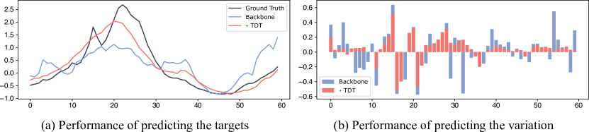
Figure 2: An example of the effect of learning TDT on the ILI dataset using the MICN model. (a) Performance of predicting the targets. (b) Performance in predicting the variation between adjacent time steps, where positive values indicate correct predictions of the increasing or decreasing relationship, while negative values indicate incorrect predictions. The magnitude of these values represents the error between the predicted and true increment or decrement values. The TDT loss helps the model better capture the dynamic associations between adjacent time steps in the predicted sequence, thereby achieving better prediction performance.

Time series inherently possess the property of temporal order, where the observations at each time step are influenced by the observations at its preceding time steps. Time series often exhibit proximity, indicating a stronger dependency on the immediately preceding step. Additionally, time series in different domains may exhibit other complex nonlinear temporal dependencies, such as periodicity, seasonality, and trend. These characteristics can be collectively referred to as temporal dependencies, which exist in both the historical sequence and the predicted sequence, i.e., targets. Temporal Dependencies among Targets (TDT) play a pivotal role in time series forecasting. First and foremost, TDT can significantly enhance the model’s predictive performance. For instance, AR models, based on the property of temporal order, recursively predict targets by conditioning on the past targets, modeling the TDT during training, and leveraging the learned TDT information during inference. Additionally, the model’s ability to capture TDT can reflect its accuracy in predicting targets. As illustrated in Figure 2, the model’s inaccurate predictions of the increasing or decreasing relationship and the specific increment or decrement values between adjacent time steps are essentially manifestations of imprecise target value predictions. Conversely, when the model achieves better target prediction performance, it also exhibits superior performance in capturing TDT.

3.2.2 Representation of TDT

To facilitate the learning of TDT by NAR models, we first need to provide a concrete representation of TDT. Considering the ubiquity of proximity in time series across various domains, we propose to define TDT as $D_{t}=\left\{d_{t+1},d_{t+2},\cdots,d_{t+H}\right\}\in\mathbb{R}^{H\times N}$, where each $d_{t+i}\in\mathbb{R}^{N}$ can be calculated by the first-order differencing [28]:

$$d_{t+i}=x_{t+i}-x_{t+i-1}.$$ (2)

$D_{t}$ can be computed using only the prediction sequence $Y_{t}$ and its immediately preceding historical time step. The value of $d_{t+i}$ quantifies the specific increment or decrement value between two adjacent time steps at a fine-grained level, while the sign of $d_{t+i}$ indicates the coarse-grained increasing or decreasing relationship between the two time steps. Consequently, $D_{t}$ provides a simple and intuitive representation of the temporal dependencies among targets at both fine-grained and coarse-grained levels. Higher-order differencing can capture more complex temporal dependencies involving more time steps. The $\tau$-order differencing results can be calculated as $d^{(\tau)}_{t+i}=d^{(\tau-1)}_{t+i}-d^{(\tau-1)}_{t+i-1}$ where $2\leq\tau\leq\min\left\{L,H\right\}$ and $d^{(1)}_{t+i}=d_{t+i}$. As $\tau$ increases, each $d^{(\tau)}_{t+i}$ involves more prediction targets, and $D^{\tau}_{t}$ requires additional historical time steps for computation. Despite the ability of higher-order differencing results to capture more complex temporal dependencies, we choose to use the first-order differencing results to represent TDT for two main reasons. First, the essential temporal dependencies are already captured by the first-order differencing results, while higher-order differencing results may not provide significant additional information and require more historical time steps, increasing computational complexity. Second, the complexity of higher-order differencing results may overshadow the lower-order dependency information and over-constrain the model, limiting the model’s learning ability and generalization performance.

We also consider an alternative approach to representing TDT, which is to use the variation between $x_{t+i}$ and $x_{t+i+k}$, where $2\leq k\leq\min\{L,H\}-1$. However, this approach has two main drawbacks. First, it would lead to the loss of information from the intermediate time steps, disregarding potentially crucial dependencies, and it also requires additional historical time steps. Second, time series exhibit strong proximity, meaning that each time step typically has the highest correlation with its immediate neighbors and lower correlation with distant time steps. By using the variation between $x_{t+i}$ and $x_{t+i+k}$, we cannot guarantee the existence of strong temporal dependencies between the time steps $t+i$ and $t+i+k$, making it less generalizable across different datasets.

The reasonableness of those two choices is further validated through experiments in Section 4.2.3. It is worth noting that the purpose and application of differencing in our work differ from most existing works [15, 29, 30, 31, 32]. In these works, differencing is typically applied to the historical data to make the time series stationary, which facilitates modeling and improves predictability. In contrast, we apply differencing to the prediction sequence, with the specific goal of representing TDT.

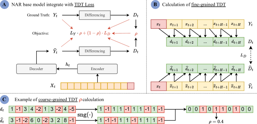
Figure 3: The proposed plug-and-play TDT Loss. (a) The TDT Loss can be seamlessly integrated into any NAR model without introducing extra learnable parameters. (b) Illustration of the fine-grained TDT calculation process. (c) An example demonstrating the computation of the $\rho$.

3.3 TDT Loss: Guiding Non-Autoregressive Models to Learn TDT

NAR base models have demonstrated remarkable effectiveness in time series forecasting tasks. However, their performance is still suboptimal due to two main limitations. First, the structural design of base models lacks explicit modeling of TDT. Second, the commonly used optimization objective in base models fails to optimize the learning of TDT. Specifically, base models typically employ an optimization objective that minimizes the discrepancy between the predicted values $\widehat{Y}_{t}$ and the ground truth $Y_{t}$:

$$\mathcal{L}_{Y}=\frac{1}{H}\sum^{H}_{i=1}{\ell(x_{t+i},\hat{x}_{t+i})},$$ (3)

where $\ell(\cdot,\cdot)$ is a distance metric such as Mean Squared Error (MSE) or Mean Absolute Error (MAE), which computes the loss for a single target or a single time step.

To tackle these challenges and improve the performance of NAR base models, we propose an innovative optimization objective called TDT Loss, which integrates TDT learning into NAR base models as depicted in Part A of Figure 3. The TDT Loss is designed to guide the base model in learning accurate predictions of targets while simultaneously capturing the intricate temporal dependencies among targets at both fine-grained and coarse-grained levels. The formulation of the TDT Loss is as follows:

$$\mathcal{L}=\rho\cdot\mathcal{L}_{Y}+(1-\rho)\cdot\mathcal{L}_{D}.$$ (4)

Target Prediction Loss ($\mathcal{L}_{Y}$) This component optimizes the base model’s ability to accurately predict the values of the targets, as defined in Equation 3.

TDT Values Prediction Loss ($\mathcal{L}_{D}$) This component measures the discrepancy between the predicted TDT values $\widehat{D}_{t}=\left\{\hat{d}_{t+1},\hat{d}_{t+2},\cdots,\hat{d}_{t+H}\right\}\in\mathbb{R}^{H\times N}$ and the ground truth $D_{t}$, as illustrated in Part B of Figure 3. It quantifies the base model’s ability to learn fine-grained TDT and is formulated as follows:

$$\mathcal{L}_{D}=\frac{1}{H}\sum^{H}_{i=1}{\ell(d_{t+i},\hat{d}_{t+i})}.$$ (5)

$\widehat{D}_{t}$ is calculated based on the predicted targets $\widehat{Y}_{t}$. The computation of $\hat{d}_{t+i}$ is defined as:

$$\hat{d}_{t+i}=\left\{\begin{array}[]{lll}\hat{x}_{t+i}-x_{t}&\mbox{if}&i=1,\\ \hat{x}_{t+i}-\hat{x}_{t+i-1}&\mbox{if}&2\leq i\leq H.\end{array}\right.$$ (6)

It should be emphasized that each $\hat{d}_{t+i}$ is computed using the predicted values of two adjacent targets. The presence of both $\mathcal{L}_{Y}$ and $\mathcal{L}_{D}$ constrains the base model to accurately predict not only the values of each target but also the dynamic associations among targets.

Adaptive Weight $\rho$ The $\rho$ represents the proportion of sign difference between the predicted TDT values $\widehat{D}_{t}$ and the ground truth $D_{t}$, as illustrated in Part C of Figure 3. It measures the base model’s ability to learn coarse-grained TDT and is defined as:

$$\rho=\frac{1}{H}\sum_{i=1}^{H}\mathbf{1}(\operatorname{sgn}(d_{t+i})\neq\operatorname{sgn}(\hat{d}_{t+i})),$$ (7)

where $\mathbf{1}(\cdot)$ is an indicator function that returns 1 if the condition is true and 0 otherwise, and $\operatorname{sgn}(\cdot)$ denotes the sign function. $\rho\in[0,1]$, and a smaller $\rho$ indicates better TDT prediction. $\rho$ enables the base model to dynamically balance its focus between target prediction and TDT learning based on its learning progress. Specifically, as the base model’s predictive capability for targets improves, $\rho$ gradually decreases, and the base model shifts its attention to learning and predicting TDT, facilitating a comprehensive understanding of the time series.

The proposed TDT Loss enables the base model to be trained end-to-end targets, coarse-grained TDT, and fine-grained TDT, leading to significant improvements in overall forecasting performance. Importantly, TDT Loss does not introduce any extra learnable parameters to base models and does not require supplementary data support. It is highly flexible and can be seamlessly integrated into existing NAR time series forecasting models. The additional costs incurred by TDT Loss are nearly negligible, with only $\mathcal{O}(n)$ increased computation and $\mathcal{O}(1)$ memory requirements, making it a highly efficient and scalable approach.

4 Experiments

In this section, we describe the experimental setup and provide experimental results along with their corresponding analyses to demonstrate the effectiveness and generality of our proposed method. We conduct ablation studies to validate the rationality of our designs.

4.1 Experimental Setup

Datasets We conduct experiments on 7 publicly available real-world datasets. These datasets cover various domains and application scenarios, including: (1) Electricity Transformer Temperature (ETT), which contains oil temperature and load data from electricity transformers and can be further divided into four sub-datasets (ETTh1, ETTh2, ETTm1, and ETTm2) based on the data collection granularity and regions; (2) Electricity, which records electricity consumption; (3) Weather, which contains various weather indicators such as temperature, humidity and wind speed; (4) Influenza-Like Illness (ILI), which collects the ratio of influenza-like illness patients versus the total patients. The statistics of these datasets are summarized in Table 1.

Table 1: Specific statistical information for 7 datasets.

Dataset	ETTh1	ETTh2	ETTm1	ETTm2	Weather	Electricity	ILI
Variables	7	7	7	7	21	321	7
Timesteps	17420	17420	69680	69680	52696	26304	966
Granularity	1 Hour	1 Hour	15 Minutes	15 Minutes	10 Minutes	1 Hour	1 Week

Various SOTA Base Models We select various open source state-of-art non-autoregressive time series forecasting models as base models and apply TDT Loss to them:(1) MLPs-based: DLinear[23] and RLinear[24], (2) CNNs-based: MICN[20] and TimesNet[21], (3) Transformers-based: PatchTST[26] and iTransformer[27]. We replace each base model’s original optimization objective with TDT Loss, keeping everything else unchanged. These base models have been introduced in section 2.

Evaluation Metrics Following the evaluation metrics used in the base models, we employ MSE and MAE to evaluate the prediction performance of targets by measuring the discrepancy between the predicted targets ($\widehat{Y}$) and the true targets ($Y$). Besides the conventional metrics, we introduce three novel metrics to assess the prediction performance of TDT at both fine-grained and coarse-grained levels by measuring the discrepancy between the predicted TDT values ($\widehat{D}$) and the true TDT values ($D$). At the fine-grained level, we use $\text{MSE}_{D}$ and $\text{MAE}_{D}$, which represent the MSE and MAE of the predicted TDT values, respectively. At the coarse-grained level, we use $\rho$ to measure the prediction error of signs of TDT values. All metrics are non-negative, with smaller values indicating smaller deviations between the predictions and trues, representing better forecasting performance.

Implementation Details To ensure fair and reliable experiments, we employ several strategies. First, we strictly follow the consistent preprocessing methods and data loading parameters from the base models to ensure the comparability of results. Based on the statistics of the training set, we employ z-score normalization to standardize the data. For dataset splitting, we adopt a 6:2:2 ratio to partition the training, validation, and test sets for the 4 ETT datasets, while the other datasets follow a 7:2:1 splitting ratio. An important aspect is that our experiments are conducted under the multivariate forecasting setting. Second, except for replacing the optimization objective with the TDT Loss, we completely follow all other configurations of the base models as described in the original papers or official code. It is worth emphasizing that we do not use the "Drop Last" operation during testing for all experiments, as suggested by [33]. Finally, all experiments are implemented using PyTorch and conducted on a single NVIDIA 4090 GPU with 24GB memory. Each experiment is conducted 5 times with 5 different random seeds.

4.2 Results and Analysis

4.2.1 Main Results

Table 2: Comparison of forecasting errors. All the results are averaged across the entire prediction horizon. The better performance are highlighted in bold. "IMP" represents the improvement percentage or quantity compared to the base model.

Methods	DLinear		+TDT		RLinear		+TDT		PatchTST		+TDT
Metric	MSE	MAE	MSE	MAE	MSE	MAE	MSE	MAE	MSE	MAE	MSE	MAE
ETTh1	0.443	0.452	0.411	0.423	0.413	0.424	0.405	0.416	0.420	0.432	0.412	0.424
ETTh2	0.460	0.459	0.407	0.420	0.353	0.397	0.350	0.386	0.343	0.386	0.348	0.386
ETTm1	0.358	0.381	0.352	0.368	0.360	0.377	0.354	0.369	0.351	0.381	0.350	0.369
ETTm2	0.281	0.340	0.259	0.315	0.256	0.313	0.257	0.309	0.257	0.314	0.256	0.309
Electricity	0.167	0.264	0.167	0.260	0.169	0.261	0.170	0.260	0.162	0.254	0.159	0.244
ILI	2.313	1.079	2.076	0.992	2.246	1.018	2.215	0.998	1.885	0.902	1.772	0.845
Weather	0.244	0.297	0.242	0.277	0.246	0.279	0.247	0.273	0.229	0.264	0.229	0.253
Model	MICN		+TDT		TimesNet		+TDT		iTransformer		+TDT
Metric	MSE	MAE	MSE	MAE	MSE	MAE	MSE	MAE	MSE	MAE	MSE	MAE
ETTh1	0.538	0.527	0.498	0.484	0.473	0.463	0.479	0.457	0.460	0.451	0.437	0.428
ETTh2	0.556	0.512	0.464	0.454	0.416	0.427	0.411	0.423	0.383	0.407	0.383	0.404
ETTm1	0.383	0.411	0.380	0.392	0.411	0.416	0.391	0.394	0.416	0.415	0.395	0.390
ETTm2	0.302	0.361	0.269	0.326	0.295	0.333	0.291	0.327	0.291	0.333	0.283	0.322
Electricity	0.189	0.296	0.181	0.281	0.196	0.296	0.232	0.311	0.176	0.267	0.180	0.263
ILI	2.785	1.141	2.710	1.095	2.340	0.961	2.126	0.900	2.287	0.967	2.395	0.988
Weather	0.250	0.307	0.233	0.264	0.262	0.289	0.259	0.282	0.260	0.280	0.255	0.271
	AVG-MSE		AVG-MAE		MAX-MSE		MAX-MAE		QUANTITY-MSE		QUANTITY-MAE
IMP	2.41%		3.90%		24.56%		16.31%		126/168		158/168

Table 2 presents the forecasting performance regarding targets of the original base models and their counterparts integrated with TDT Loss ("+TDT" in the table). The detailed results of all cases, including the mean and standard deviation of the results from 5 runs for each forecast horizon, are provided in Appendix A.2. Out of a total of 168 experiments, 75.00% demonstrate improvements in MSE, and 94.05% in MAE with TDT Loss. The average improvements in MSE and MAE are 2.41% and 3.90%, respectively. Some remarkable achievements are: (1) The maximum improvements in MSE and MAE are 24.56% and 16.31%, respectively. (2) MICN achieves the highest average improvements in MSE and MAE, reaching 6.55% and 7.99%, respectively, followed by DLinear with 5.12% and 5.90%. (3) 85.71% of the experiments exhibit significantly reduced standard deviations in both MSE and MAE, indicating that the predictions of the base models become more stable with TDT Loss. These findings can be observed in Table 7, Table 8 and Table 9.

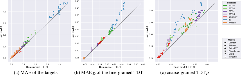
Figure 4: Forecasting performance of the original base models and their counterparts integrated with TDT Loss across 168 experiments. Points above the diagonal line signify improved performance with the TDT Loss. The results demonstrate the effectiveness of the TDT Loss in enhancing the prediction of targets, fine-grained TDT and coarse-grained TDT.

4.2.2 Efficiency Analysis

Figure 4 illustrates the forecasting performance of the original base models and their counterparts integrated with TDT Loss on (a) targets, (b) fine-grained TDT, i.e., TDT values, and (c) coarse-grained TDT, i.e., the signs of TDT values. For brevity, we only discuss the mean absolute error for both targets and fine-grained TDT predictions. The detailed results of all cases about targets, fine-grained TDT, and coarse-grained TDT, including the mean and standard deviation of the metrics from 5 runs for each forecast horizon, are provided in Appendix A.3. With TDT Loss, out of a total of 168 experiments, 94.05%, 100.00%, and 99.40% of the experiments exhibit improvements in targets, fine-grained TDT, and coarse-grained TDT predictions, respectively. Among the experiments with enhanced coarse-grained TDT prediction, all achieve better fine-grained TDT prediction, and 94.61% attain improved target prediction. This verifies that learning TDT can enhance the base models’ prediction capability for targets, and the prediction performance of TDT can also reflect the base models’ prediction capability for targets. On the other hand, among the experiments with better target prediction, all demonstrate improvements in fine-grained TDT and coarse-grained TDT prediction, verifying that if the base models forecast targets well, they also perform well in TDT prediction.

4.2.3 Ablation Study

Table 3: Comparison of forecasting errors with different orders ($\tau$). The best performance are highlighted in bold.

$H$	iTransformer		$\tau=1$		$\tau=2$		$\tau=3$		$\tau=4$
	MAE	MSE	MAE	MSE	MAE	MSE	MAE	MSE	MAE	MSE
96	0.389	0.407	0.375	0.389	0.377	0.390	0.380	0.392	0.388	0.401
192	0.446	0.439	0.428	0.419	0.430	0.420	0.433	0.425	0.445	0.437
336	0.488	0.460	0.470	0.442	0.470	0.442	0.478	0.451	0.501	0.469
720	0.516	0.496	0.474	0.463	0.468	0.463	0.489	0.483	0.544	0.514

To validate the effectiveness of our design choices, we conduct ablation experiments with five different TDT Loss configurations: (1) Comparing the effects of using the differencing results with different orders to represent TDT, setting $\tau\in\{1,2,3,4\}$. (2) Comparing the effects of using variations between $x_{t+i}$ and $x_{t+i+k}$ with different step sizes $k$ to represent TDT, setting $k\in\{1,2,3,4,5,6\}$. (3) Comparing the effects of $\rho$ and the adaptive learning weight $\alpha$. (4) Evaluating the impact of fine-grained TDT learning by removing $\mathcal{L}_{D}$, corresponding optimization objective: $\mathcal{L}=\rho\cdot\mathcal{L}_{Y}$, (5) Evaluating the impact of coarse-grained TDT learning by removing $\rho$, corresponding optimization objective: $\mathcal{L}=\mathcal{L}_{Y}+\mathcal{L}_{D}$. All ablation experiments employ iTransformer as the base model and are conducted on the ETTh1 dataset, with the prediction performance evaluated on the targets. These experiments only report the mean values to save space. The detailed results of all ablation studies, including the mean and standard deviation of the metrics across 5 runs for each forecasting horizon, are provided in Appendix A.4.

Table 3 demonstrates that employing the first-order differencing results ($\tau=1$) to represent TDT achieves the best prediction performance. This suggests that the first-order differencing results can provide adequate and easily learnable information for the base models. In contrast, higher-order differencing results do not contribute additional information and may instead over-constrain the models, leading to a decrease in performance.

Table 4: Comparison of forecasting errors with different time step ($k$). The best performance are highlighted in bold.

$H$	iTransformer		$k=1$		$k=2$		$k=3$		$k=4$		$k=5$		$k=6$
	MAE	MSE	MAE	MSE	MAE	MSE	MAE	MSE	MAE	MSE	MAE	MSE	MAE	MSE
96	0.389	0.407	0.375	0.389	0.374	0.388	0.377	0.390	0.378	0.391	0.380	0.392	0.382	0.394
192	0.446	0.439	0.428	0.419	0.428	0.420	0.432	0.422	0.433	0.422	0.435	0.423	0.437	0.424
336	0.488	0.460	0.470	0.442	0.470	0.441	0.473	0.442	0.474	0.442	0.478	0.444	0.480	0.447
720	0.516	0.496	0.474	0.463	0.477	0.463	0.485	0.466	0.487	0.464	0.492	0.466	0.493	0.466

Table 4 demonstrates that utilizing the variations between adjacent time steps ($k=1$) to represent TDT achieves the best prediction performance. Furthermore, as the step size increases, the prediction performance progressively declines. This suggests that larger time intervals may overlook valuable information from intermediate time steps and exhibit weaker dependency relationships compared to those between adjacent time steps.

Table 5 demonstrates that $\rho$ better captures the learning progress of the base models and provides more effective guidance for adjusting their learning focus compared to the adaptive learning weight $\alpha$. The results also show that learning either fine-grained or coarse-grained TDT alone can moderately enhance the prediction performance of base models. However, learning both fine-grained and coarse-grained TDT simultaneously enables the base models to achieve the best prediction performance, emphasizing the necessity and effectiveness of learning TDT.

Table 5: Comparison of forecasting errors on ablative variants. The best performance are highlighted in bold.

$H$	iTransformer		+TDT		$\alpha$		w/o $\mathcal{L}_{D}$		w/o $\rho$
	MAE	MSE	MAE	MSE	MAE	MSE	MAE	MSE	MAE	MSE
96	0.389	0.407	0.375	0.389	0.377	0.391	0.388	0.400	0.379	0.392
192	0.446	0.439	0.428	0.419	0.430	0.422	0.439	0.429	0.432	0.422
336	0.488	0.460	0.470	0.442	0.474	0.445	0.479	0.448	0.472	0.444
720	0.516	0.496	0.474	0.463	0.490	0.472	0.505	0.480	0.495	0.475

5 Conclusion

In this study, we argued that integrating temporal dependencies among targets (TDT) learning into non-autoregressive time series prediction models can leverage the strengths of both autoregressive and non-autoregressive paradigms. To achieve this goal, we proposed a novel optimization objective, the TDT Loss, as a parameter-free, plug-and-play solution with negligible additional costs. The TDT Loss guided the model to learn TDT and dynamically adjust the focus between learning future sequence predictions and learning TDT. To demonstrate the effectiveness and generality of the TDT Loss, we conducted experiments on widely-used datasets and found that the TDT Loss significantly improved the prediction performance of state-of-the-art time series prediction models. Lastly, we discussed the limitations of the TDT Loss and potential future research directions in Appendix B. We hope that the TDT Loss will inspire further research on time series modeling from the perspective of learning temporal dependencies among targets.

Appendix A Additional Results

A.1 Other Implementation Details

In the experimental setup, we strictly adhere to the original settings of each base model regarding the input historical sequence length and the forecasting horizon to ensure the fairness and comparability of the experimental results. The required input historical sequence length may vary across different base models, depending on their respective model architectures and training strategies, but they have a consistent forecasting horizon. Table 6 summarizes the specific configurations of the input historical sequence length and the forecasting horizon for each base model on different datasets.

Table 6: Configurations of input historical sequence length and forecasting horizon.

Base Models	ILI	Other Datasets
	L $\Rightarrow$ H	L $\Rightarrow$ H
DLinear, RLinear, PatchTST	104 $\Rightarrow$ {24, 36, 48, 60}	336 $\Rightarrow$ {96, 192, 336, 720}
iTransformer, MICN, TimesNet	36 $\Rightarrow$ {24, 36, 48, 60}	96 $\Rightarrow$ {96, 192, 336, 720}

A.2 Full Main Results

Table 7: Full results on MLPs-based models.

Model		DLinear		+TDT		RLinear		+TDT
Metric		MSE	MAE	MSE	MAE	MSE	MAE	MSE	MAE
ETTh1	96	0.376±0.005	0.399±0.006	0.362±0.000	0.384±0.000	0.371±0.001	0.393±0.001	0.362±0.000	0.385±0.000
	192	0.407±0.003	0.416±0.003	0.400±0.000	0.407±0.000	0.403±0.000	0.412±0.000	0.400±0.000	0.407±0.000
	336	0.490±0.041	0.485±0.033	0.431±0.000	0.427±0.000	0.428±0.000	0.427±0.000	0.427±0.000	0.423±0.000
	720	0.498±0.021	0.508±0.015	0.453±0.000	0.473±0.000	0.449±0.001	0.462±0.001	0.432±0.000	0.449±0.000
ETTh2	96	0.294±0.006	0.357±0.005	0.278±0.000	0.333±0.000	0.274±0.001	0.338±0.000	0.279±0.000	0.333±0.000
	192	0.376±0.005	0.412±0.005	0.352±0.000	0.385±0.000	0.338±0.002	0.384±0.001	0.345±0.000	0.377±0.000
	336	0.458±0.010	0.466±0.005	0.410±0.000	0.429±0.000	0.369±0.003	0.412±0.001	0.374±0.000	0.404±0.000
	720	0.714±0.019	0.601±0.006	0.587±0.001	0.533±0.000	0.431±0.007	0.453±0.004	0.402±0.000	0.431±0.000
ETTm1	96	0.301±0.001	0.345±0.002	0.292±0.000	0.333±0.000	0.304±0.003	0.345±0.002	0.294±0.000	0.334±0.000
	192	0.336±0.001	0.367±0.001	0.331±0.000	0.355±0.000	0.337±0.001	0.364±0.001	0.332±0.000	0.357±0.000
	336	0.371±0.003	0.389±0.004	0.365±0.000	0.376±0.000	0.371±0.002	0.383±0.002	0.366±0.000	0.377±0.000
	720	0.426±0.002	0.422±0.003	0.420±0.000	0.410±0.000	0.429±0.005	0.417±0.003	0.423±0.000	0.410±0.000
ETTm2	96	0.170±0.002	0.264±0.002	0.164±0.000	0.247±0.000	0.164±0.000	0.253±0.000	0.164±0.000	0.247±0.000
	192	0.229±0.005	0.306±0.007	0.221±0.000	0.287±0.000	0.219±0.000	0.290±0.000	0.221±0.000	0.286±0.000
	336	0.288±0.005	0.349±0.007	0.276±0.000	0.329±0.000	0.272±0.000	0.325±0.000	0.275±0.000	0.322±0.000
	720	0.438±0.072	0.442±0.042	0.374±0.000	0.395±0.000	0.368±0.001	0.385±0.000	0.368±0.000	0.380±0.000
Electricity	96	0.140±0.000	0.237±0.000	0.141±0.000	0.235±0.000	0.141±0.000	0.236±0.000	0.142±0.000	0.235±0.000
	192	0.154±0.000	0.250±0.000	0.154±0.000	0.247±0.000	0.155±0.000	0.248±0.000	0.156±0.000	0.247±0.000
	336	0.169±0.000	0.268±0.000	0.170±0.000	0.263±0.000	0.171±0.000	0.265±0.000	0.172±0.000	0.263±0.000
	720	0.204±0.000	0.301±0.000	0.204±0.000	0.294±0.000	0.210±0.000	0.297±0.000	0.211±0.000	0.295±0.000
ILI	24	2.265±0.064	1.048±0.027	2.163±0.002	0.992±0.001	2.365±0.113	1.044±0.039	2.308±0.022	1.013±0.006
	36	2.251±0.107	1.064±0.049	2.055±0.004	0.981±0.002	2.195±0.027	1.000±0.010	2.195±0.021	0.987±0.007
	48	2.302±0.021	1.082±0.007	2.017±0.004	0.983±0.002	2.211±0.074	1.012±0.026	2.162±0.007	0.986±0.002
	60	2.435±0.024	1.120±0.009	2.070±0.008	1.012±0.003	2.214±0.099	1.014±0.031	2.193±0.011	1.006±0.003
Weather	96	0.175±0.001	0.238±0.003	0.174±0.000	0.218±0.000	0.174±0.000	0.224±0.000	0.175±0.000	0.215±0.000
	192	0.216±0.001	0.274±0.001	0.214±0.000	0.255±0.000	0.217±0.000	0.259±0.000	0.217±0.000	0.252±0.000
	336	0.262±0.002	0.313±0.003	0.259±0.000	0.292±0.000	0.264±0.000	0.293±0.000	0.265±0.000	0.288±0.000
	720	0.325±0.001	0.364±0.001	0.320±0.000	0.343±0.000	0.331±0.000	0.339±0.000	0.333±0.000	0.336±0.000

Table 8: Full results on Transformers-based models.

Model		PatchTST		+TDT		iTransformer		+TDT
Metric		MSE	MAE	MSE	MAE	MSE	MAE	MSE	MAE
ETTh1	96	0.380±0.001	0.402±0.001	0.373±0.001	0.396±0.001	0.389±0.002	0.407±0.001	0.375±0.001	0.389±0.000
	192	0.412±0.000	0.420±0.000	0.409±0.001	0.417±0.001	0.446±0.002	0.439±0.002	0.428±0.001	0.419±0.001
	336	0.436±0.003	0.437±0.003	0.433±0.001	0.431±0.001	0.488±0.002	0.460±0.001	0.470±0.002	0.442±0.002
	720	0.453±0.003	0.469±0.002	0.433±0.002	0.453±0.002	0.516±0.007	0.496±0.004	0.474±0.008	0.463±0.005
ETTh2	96	0.276±0.001	0.338±0.001	0.277±0.000	0.334±0.000	0.299±0.002	0.350±0.001	0.295±0.001	0.344±0.000
	192	0.340±0.001	0.380±0.001	0.346±0.001	0.378±0.001	0.380±0.002	0.399±0.001	0.380±0.001	0.395±0.000
	336	0.364±0.003	0.399±0.001	0.375±0.001	0.404±0.001	0.423±0.002	0.432±0.001	0.427±0.001	0.431±0.001
	720	0.391±0.001	0.429±0.001	0.395±0.001	0.427±0.000	0.431±0.003	0.448±0.001	0.429±0.002	0.444±0.001
ETTm1	96	0.290±0.001	0.342±0.000	0.290±0.002	0.327±0.001	0.333±0.003	0.369±0.002	0.316±0.001	0.347±0.000
	192	0.331±0.002	0.368±0.001	0.335±0.002	0.358±0.001	0.389±0.011	0.398±0.006	0.371±0.001	0.374±0.001
	336	0.366±0.001	0.391±0.001	0.360±0.006	0.379±0.002	0.436±0.011	0.427±0.005	0.414±0.002	0.401±0.001
	720	0.417±0.003	0.423±0.002	0.414±0.005	0.411±0.003	0.506±0.006	0.467±0.002	0.479±0.003	0.438±0.002
ETTm2	96	0.164±0.000	0.253±0.001	0.165±0.003	0.247±0.002	0.182±0.001	0.265±0.001	0.177±0.001	0.254±0.000
	192	0.221±0.001	0.292±0.001	0.221±0.002	0.286±0.001	0.252±0.004	0.311±0.002	0.244±0.001	0.298±0.001
	336	0.276±0.001	0.329±0.001	0.273±0.002	0.321±0.001	0.314±0.003	0.350±0.002	0.306±0.002	0.338±0.001
	720	0.367±0.001	0.384±0.001	0.363±0.007	0.383±0.005	0.415±0.007	0.408±0.004	0.405±0.003	0.396±0.001
Electricity	96	0.130±0.000	0.223±0.000	0.130±0.000	0.216±0.000	0.148±0.000	0.240±0.000	0.152±0.000	0.237±0.000
	192	0.149±0.001	0.241±0.001	0.147±0.000	0.232±0.000	0.164±0.001	0.255±0.001	0.168±0.001	0.251±0.001
	336	0.166±0.001	0.260±0.001	0.162±0.000	0.247±0.000	0.179±0.001	0.272±0.001	0.183±0.001	0.267±0.000
	720	0.203±0.001	0.292±0.001	0.197±0.000	0.279±0.000	0.213±0.009	0.302±0.007	0.216±0.001	0.296±0.001
ILI	24	2.050±0.087	0.917±0.026	1.819±0.091	0.834±0.031	2.354±0.018	0.952±0.007	2.543±0.028	1.007±0.007
	36	1.905±0.086	0.895±0.046	1.759±0.058	0.839±0.025	2.234±0.033	0.959±0.006	2.331±0.008	0.976±0.003
	48	1.802±0.119	0.900±0.031	1.746±0.091	0.848±0.026	2.269±0.057	0.971±0.015	2.326±0.010	0.977±0.003
	60	1.785±0.159	0.897±0.063	1.764±0.049	0.861±0.014	2.289±0.025	0.987±0.004	2.381±0.010	0.994±0.003
Weather	96	0.150±0.001	0.198±0.001	0.152±0.000	0.187±0.000	0.175±0.001	0.215±0.001	0.169±0.001	0.202±0.001
	192	0.195±0.001	0.241±0.001	0.196±0.000	0.230±0.000	0.225±0.001	0.258±0.001	0.219±0.001	0.247±0.001
	336	0.248±0.001	0.282±0.001	0.248±0.001	0.271±0.001	0.282±0.001	0.299±0.001	0.278±0.001	0.292±0.001
	720	0.321±0.001	0.334±0.001	0.322±0.000	0.325±0.000	0.358±0.001	0.350±0.001	0.356±0.001	0.344±0.000

Table 9: Full results on CNNs-based models.

Model		MICN		+TDT		TimesNet		+TDT
Metric		MSE	MAE	MSE	MAE	MSE	MAE	MSE	MAE
ETTh1	96	0.412±0.010	0.437±0.009	0.387±0.005	0.407±0.004	0.407±0.014	0.424±0.009	0.407±0.008	0.419±0.006
	192	0.482±0.010	0.484±0.006	0.446±0.014	0.443±0.010	0.458±0.011	0.453±0.007	0.457±0.015	0.443±0.008
	336	0.574±0.026	0.553±0.014	0.493±0.012	0.482±0.003	0.513±0.008	0.482±0.004	0.522±0.056	0.472±0.022
	720	0.686±0.089	0.632±0.050	0.666±0.056	0.604±0.031	0.516±0.009	0.493±0.005	0.530±0.086	0.492±0.037
ETTh2	96	0.312±0.014	0.368±0.015	0.299±0.005	0.352±0.007	0.321±0.009	0.364±0.005	0.315±0.004	0.356±0.003
	192	0.437±0.044	0.455±0.032	0.379±0.006	0.404±0.006	0.427±0.024	0.428±0.014	0.418±0.011	0.422±0.009
	336	0.623±0.099	0.558±0.047	0.470±0.012	0.467±0.005	0.463±0.015	0.457±0.011	0.446±0.014	0.448±0.011
	720	0.850±0.047	0.666±0.023	0.709±0.042	0.593±0.017	0.452±0.021	0.461±0.014	0.464±0.001	0.467±0.001
ETTm1	96	0.312±0.002	0.362±0.004	0.310±0.004	0.342±0.001	0.336±0.004	0.375±0.003	0.328±0.006	0.359±0.005
	192	0.356±0.002	0.391±0.003	0.361±0.003	0.378±0.003	0.395±0.011	0.405±0.007	0.371±0.006	0.382±0.004
	336	0.394±0.008	0.421±0.005	0.387±0.006	0.399±0.006	0.420±0.009	0.423±0.003	0.400±0.002	0.400±0.003
	720	0.469±0.009	0.471±0.008	0.461±0.006	0.450±0.009	0.493±0.004	0.462±0.003	0.464±0.004	0.435±0.003
ETTm2	96	0.176±0.001	0.272±0.002	0.171±0.001	0.257±0.001	0.187±0.003	0.266±0.001	0.180±0.001	0.257±0.001
	192	0.257±0.012	0.335±0.011	0.232±0.001	0.300±0.002	0.252±0.001	0.308±0.001	0.246±0.001	0.300±0.001
	336	0.312±0.016	0.369±0.015	0.292±0.006	0.344±0.005	0.317±0.005	0.347±0.002	0.311±0.002	0.340±0.001
	720	0.464±0.012	0.466±0.008	0.380±0.005	0.401±0.005	0.423±0.007	0.409±0.007	0.425±0.009	0.411±0.010
Electricity	96	0.162±0.005	0.269±0.003	0.158±0.002	0.260±0.003	0.169±0.003	0.272±0.003	0.173±0.004	0.268±0.004
	192	0.179±0.003	0.286±0.003	0.170±0.002	0.271±0.002	0.186±0.002	0.288±0.002	0.203±0.023	0.291±0.014
	336	0.200±0.006	0.309±0.006	0.185±0.005	0.286±0.004	0.200±0.005	0.300±0.004	0.258±0.003	0.329±0.003
	720	0.213±0.005	0.322±0.006	0.212±0.005	0.309±0.004	0.230±0.009	0.324±0.008	0.294±0.003	0.357±0.003
ILI	24	2.752±0.037	1.147±0.010	2.811±0.024	1.135±0.005	2.327±0.399	0.949±0.057	2.077±0.196	0.901±0.035
	36	2.748±0.024	1.138±0.007	2.714±0.026	1.102±0.008	2.582±0.166	1.005±0.018	2.128±0.084	0.900±0.019
	48	2.772±0.050	1.131±0.012	2.638±0.011	1.068±0.003	2.296±0.066	0.943±0.022	2.167±0.092	0.896±0.021
	60	2.870±0.062	1.149±0.012	2.675±0.015	1.076±0.004	2.154±0.072	0.945±0.010	2.131±0.063	0.903±0.014
Weather	96	0.170±0.003	0.236±0.005	0.158±0.001	0.199±0.002	0.172±0.001	0.222±0.001	0.172±0.004	0.216±0.004
	192	0.225±0.007	0.292±0.010	0.208±0.002	0.246±0.003	0.232±0.006	0.271±0.005	0.226±0.004	0.262±0.002
	336	0.270±0.012	0.326±0.013	0.252±0.002	0.283±0.002	0.285±0.004	0.307±0.003	0.283±0.002	0.302±0.002
	720	0.335±0.013	0.375±0.015	0.312±0.003	0.329±0.003	0.360±0.002	0.355±0.001	0.356±0.001	0.350±0.001

We provide comprehensive and detailed experimental results of the comparison between base models and their counterparts enhanced with TDT Loss, as a supplementary explanation to Table 2. All experiments are conducted 5 times with 5 different random seeds.

Table 7, Table 8 and Table 9 clearly present the experimental results of different base models on various datasets. Based on these results, we observe that TDT Loss can improve the forecasting performance of base models in most cases. In particular, the overall enhancement effect is significant for DLinear and MICN models. Moreover, on the ETTh1 and Weather datasets, all base models exhibit improved performance after incorporating TDT Loss.

Moreover, it is worth noting that after applying TDT Loss, base models not only achieve better forecasting performance but also demonstrate smaller standard deviations. This indicates that TDT Loss can effectively enhance the stability of the forecasting performance of base models.

A.3 Full Results of Efficiency Analysis

Table 10: Full results of $\text{MSE}_{D}$ and $\text{MAE}_{D}$ on MLPs-based models.

Model		DLinear		+TDT		RLinear		+TDT
Metric		$\text{MSE}_{D}$	$\text{MAE}_{D}$	$\text{MSE}_{D}$	$\text{MAE}_{D}$	$\text{MSE}_{D}$	$\text{MAE}_{D}$	$\text{MSE}_{D}$	$\text{MAE}_{D}$
ETTh1	96	0.114±0.001	0.214±0.003	0.111±0.000	0.209±0.000	0.113±0.000	0.212±0.001	0.111±0.000	0.210±0.000
	192	0.116±0.001	0.217±0.001	0.115±0.000	0.214±0.000	0.116±0.000	0.216±0.000	0.115±0.000	0.214±0.000
	336	0.129±0.007	0.237±0.012	0.119±0.000	0.218±0.000	0.120±0.000	0.220±0.000	0.119±0.000	0.219±0.000
	720	0.125±0.005	0.230±0.010	0.120±0.000	0.220±0.000	0.121±0.000	0.223±0.001	0.120±0.000	0.220±0.000
ETTh2	96	0.078±0.001	0.170±0.003	0.076±0.000	0.163±0.000	0.079±0.000	0.168±0.001	0.076±0.000	0.159±0.000
	192	0.079±0.001	0.170±0.003	0.077±0.000	0.164±0.000	0.080±0.000	0.169±0.000	0.077±0.000	0.161±0.000
	336	0.086±0.010	0.179±0.013	0.078±0.000	0.165±0.000	0.081±0.001	0.171±0.002	0.078±0.000	0.162±0.000
	720	0.081±0.000	0.170±0.001	0.079±0.000	0.165±0.000	0.090±0.008	0.184±0.014	0.080±0.000	0.163±0.000
ETTm1	96	0.049±0.000	0.133±0.001	0.049±0.000	0.132±0.000	0.049±0.000	0.133±0.001	0.049±0.000	0.132±0.000
	192	0.050±0.000	0.134±0.000	0.049±0.000	0.133±0.000	0.050±0.000	0.134±0.001	0.050±0.000	0.133±0.000
	336	0.050±0.000	0.135±0.001	0.050±0.000	0.134±0.000	0.050±0.000	0.134±0.001	0.050±0.000	0.134±0.000
	720	0.051±0.000	0.136±0.000	0.051±0.000	0.136±0.000	0.051±0.000	0.137±0.001	0.051±0.000	0.135±0.000
ETTm2	96	0.035±0.001	0.101±0.003	0.034±0.000	0.093±0.000	0.034±0.000	0.094±0.000	0.034±0.000	0.092±0.000
	192	0.035±0.001	0.100±0.003	0.034±0.000	0.093±0.000	0.034±0.000	0.094±0.000	0.034±0.000	0.092±0.000
	336	0.035±0.001	0.100±0.003	0.034±0.000	0.093±0.000	0.034±0.000	0.094±0.000	0.034±0.000	0.092±0.000
	720	0.039±0.004	0.111±0.011	0.034±0.000	0.093±0.000	0.034±0.000	0.094±0.000	0.034±0.000	0.092±0.000
Electricity	96	0.059±0.000	0.150±0.000	0.059±0.000	0.149±0.000	0.059±0.000	0.150±0.000	0.059±0.000	0.149±0.000
	192	0.061±0.000	0.152±0.000	0.061±0.000	0.151±0.000	0.061±0.000	0.153±0.000	0.061±0.000	0.151±0.000
	336	0.063±0.000	0.155±0.000	0.063±0.000	0.154±0.000	0.063±0.000	0.156±0.000	0.063±0.000	0.154±0.000
	720	0.068±0.000	0.162±0.000	0.069±0.000	0.161±0.000	0.069±0.000	0.163±0.000	0.069±0.000	0.161±0.000
ILI	24	0.207±0.008	0.265±0.011	0.189±0.001	0.239±0.000	0.418±0.091	0.438±0.057	0.278±0.007	0.320±0.004
	36	0.207±0.004	0.262±0.008	0.188±0.000	0.235±0.001	0.361±0.018	0.399±0.012	0.274±0.007	0.314±0.005
	48	0.203±0.000	0.251±0.001	0.189±0.000	0.234±0.000	0.414±0.070	0.432±0.044	0.271±0.003	0.313±0.002
	60	0.210±0.003	0.258±0.004	0.193±0.000	0.236±0.000	0.391±0.071	0.416±0.047	0.272±0.004	0.312±0.003
Weather	96	0.039±0.000	0.042±0.000	0.038±0.000	0.041±0.000	0.039±0.000	0.041±0.000	0.039±0.000	0.041±0.000
	192	0.039±0.000	0.041±0.000	0.039±0.000	0.041±0.000	0.039±0.000	0.041±0.000	0.039±0.000	0.041±0.000
	336	0.039±0.000	0.042±0.000	0.039±0.000	0.041±0.000	0.039±0.000	0.041±0.000	0.039±0.000	0.041±0.000
	720	0.040±0.000	0.041±0.000	0.040±0.000	0.041±0.000	0.040±0.000	0.041±0.000	0.040±0.000	0.041±0.000

Table 11: Full results of $\text{MSE}_{D}$ and $\text{MAE}_{D}$ on Transformers-based models.

Model		PatchTST		+TDT		iTransformer		+TDT
Metric		$\text{MSE}_{D}$	$\text{MAE}_{D}$	$\text{MSE}_{D}$	$\text{MAE}_{D}$	$\text{MSE}_{D}$	$\text{MAE}_{D}$	$\text{MSE}_{D}$	$\text{MAE}_{D}$
ETTh1	96	0.131±0.001	0.232±0.001	0.124±0.000	0.223±0.000	0.127±0.001	0.231±0.001	0.115±0.000	0.213±0.000
	192	0.134±0.001	0.236±0.000	0.128±0.001	0.227±0.001	0.136±0.001	0.240±0.001	0.121±0.000	0.219±0.000
	336	0.140±0.003	0.243±0.004	0.131±0.001	0.230±0.001	0.148±0.005	0.253±0.005	0.127±0.000	0.225±0.000
	720	0.157±0.006	0.263±0.007	0.132±0.001	0.233±0.001	0.157±0.005	0.263±0.005	0.129±0.000	0.229±0.000
ETTh2	96	0.083±0.000	0.169±0.000	0.079±0.000	0.160±0.000	0.092±0.000	0.184±0.001	0.083±0.000	0.166±0.000
	192	0.087±0.001	0.177±0.003	0.080±0.000	0.161±0.000	0.092±0.000	0.184±0.001	0.084±0.000	0.167±0.000
	336	0.086±0.000	0.174±0.001	0.081±0.000	0.163±0.001	0.094±0.001	0.186±0.001	0.086±0.000	0.168±0.000
	720	0.088±0.001	0.175±0.002	0.083±0.000	0.165±0.001	0.096±0.001	0.188±0.002	0.088±0.000	0.169±0.000
ETTm1	96	0.051±0.000	0.140±0.000	0.050±0.000	0.135±0.000	0.053±0.000	0.143±0.001	0.050±0.000	0.134±0.000
	192	0.052±0.000	0.140±0.000	0.050±0.000	0.136±0.000	0.054±0.000	0.145±0.001	0.050±0.000	0.134±0.000
	336	0.053±0.001	0.143±0.001	0.051±0.000	0.136±0.000	0.055±0.000	0.147±0.001	0.051±0.000	0.135±0.000
	720	0.054±0.001	0.146±0.001	0.052±0.000	0.138±0.000	0.056±0.000	0.148±0.000	0.052±0.000	0.137±0.000
ETTm2	96	0.037±0.000	0.107±0.001	0.034±0.000	0.093±0.000	0.036±0.000	0.102±0.000	0.034±0.000	0.093±0.000
	192	0.039±0.000	0.113±0.000	0.034±0.000	0.093±0.001	0.036±0.000	0.103±0.001	0.034±0.000	0.093±0.000
	336	0.041±0.001	0.119±0.001	0.034±0.000	0.093±0.000	0.036±0.000	0.101±0.001	0.035±0.000	0.093±0.000
	720	0.041±0.001	0.119±0.002	0.034±0.000	0.094±0.001	0.037±0.000	0.102±0.001	0.035±0.000	0.092±0.000
Electricity	96	0.058±0.000	0.148±0.000	0.056±0.000	0.142±0.000	0.067±0.000	0.161±0.000	0.065±0.000	0.156±0.000
	192	0.060±0.000	0.151±0.000	0.058±0.000	0.144±0.000	0.067±0.000	0.161±0.000	0.066±0.000	0.157±0.000
	336	0.062±0.000	0.154±0.000	0.060±0.000	0.147±0.000	0.069±0.000	0.164±0.000	0.068±0.000	0.159±0.000
	720	0.068±0.000	0.162±0.000	0.065±0.000	0.154±0.000	0.075±0.001	0.173±0.003	0.073±0.000	0.166±0.000
ILI	24	0.228±0.010	0.285±0.012	0.191±0.004	0.242±0.003	0.259±0.003	0.316±0.004	0.231±0.002	0.272±0.003
	36	0.222±0.007	0.274±0.007	0.190±0.004	0.236±0.003	0.259±0.005	0.313±0.004	0.230±0.000	0.265±0.001
	48	0.223±0.015	0.274±0.018	0.189±0.002	0.234±0.002	0.263±0.012	0.317±0.012	0.231±0.002	0.264±0.003
	60	0.217±0.014	0.265±0.015	0.191±0.002	0.235±0.001	0.260±0.003	0.311±0.003	0.236±0.001	0.264±0.001
Weather	96	0.039±0.000	0.044±0.000	0.039±0.000	0.040±0.000	0.039±0.000	0.046±0.000	0.039±0.000	0.041±0.000
	192	0.039±0.000	0.044±0.000	0.039±0.000	0.040±0.000	0.039±0.000	0.047±0.000	0.039±0.000	0.041±0.000
	336	0.039±0.000	0.045±0.001	0.039±0.000	0.040±0.000	0.040±0.000	0.048±0.000	0.039±0.000	0.041±0.000
	720	0.040±0.000	0.046±0.001	0.040±0.000	0.040±0.000	0.041±0.000	0.049±0.000	0.040±0.000	0.041±0.000

Table 12: Full results of $\text{MSE}_{D}$ and $\text{MAE}_{D}$ on CNNs-based models.

Model		MICN		+TDT		TimesNet		+TDT
Metric		$\text{MSE}_{D}$	$\text{MAE}_{D}$	$\text{MSE}_{D}$	$\text{MAE}_{D}$	$\text{MSE}_{D}$	$\text{MAE}_{D}$	$\text{MSE}_{D}$	$\text{MAE}_{D}$
ETTh1	96	0.128±0.001	0.233±0.001	0.117±0.001	0.217±0.001	0.141±0.005	0.244±0.005	0.138±0.003	0.236±0.002
	192	0.130±0.002	0.235±0.001	0.122±0.001	0.221±0.001	0.144±0.004	0.246±0.003	0.144±0.006	0.241±0.005
	336	0.132±0.001	0.237±0.002	0.126±0.001	0.226±0.001	0.154±0.001	0.255±0.001	0.154±0.010	0.249±0.006
	720	0.134±0.001	0.240±0.001	0.130±0.002	0.232±0.002	0.155±0.003	0.258±0.002	0.154±0.012	0.249±0.006
ETTh2	96	0.082±0.001	0.172±0.003	0.079±0.001	0.169±0.001	0.091±0.002	0.181±0.003	0.083±0.000	0.162±0.001
	192	0.082±0.002	0.172±0.002	0.080±0.001	0.170±0.002	0.099±0.011	0.194±0.017	0.086±0.001	0.164±0.001
	336	0.083±0.001	0.174±0.003	0.081±0.001	0.172±0.001	0.098±0.008	0.192±0.014	0.086±0.001	0.164±0.000
	720	0.085±0.001	0.175±0.002	0.082±0.001	0.173±0.001	0.096±0.005	0.188±0.011	0.089±0.000	0.166±0.000
ETTm1	96	0.053±0.001	0.142±0.001	0.050±0.000	0.136±0.000	0.055±0.000	0.146±0.001	0.052±0.000	0.137±0.001
	192	0.052±0.000	0.142±0.001	0.050±0.000	0.137±0.000	0.055±0.001	0.146±0.002	0.052±0.000	0.137±0.000
	336	0.052±0.001	0.142±0.001	0.050±0.000	0.136±0.000	0.056±0.001	0.147±0.001	0.052±0.000	0.137±0.000
	720	0.053±0.000	0.143±0.001	0.051±0.000	0.137±0.001	0.056±0.000	0.147±0.001	0.053±0.000	0.139±0.000
ETTm2	96	0.036±0.000	0.105±0.001	0.035±0.000	0.099±0.001	0.037±0.000	0.104±0.001	0.035±0.000	0.092±0.000
	192	0.036±0.001	0.105±0.002	0.035±0.000	0.099±0.001	0.038±0.001	0.107±0.003	0.035±0.000	0.092±0.000
	336	0.035±0.000	0.103±0.003	0.034±0.000	0.098±0.001	0.037±0.000	0.102±0.000	0.035±0.000	0.092±0.000
	720	0.037±0.001	0.106±0.005	0.034±0.000	0.096±0.001	0.037±0.001	0.103±0.002	0.035±0.000	0.091±0.001
Electricity	96	0.079±0.001	0.183±0.001	0.077±0.001	0.175±0.001	0.083±0.001	0.189±0.002	0.081±0.001	0.179±0.001
	192	0.083±0.002	0.188±0.002	0.077±0.001	0.175±0.001	0.085±0.003	0.191±0.002	0.083±0.002	0.181±0.002
	336	0.085±0.003	0.191±0.004	0.078±0.001	0.176±0.001	0.085±0.001	0.192±0.002	0.087±0.000	0.185±0.001
	720	0.085±0.000	0.190±0.001	0.080±0.000	0.177±0.000	0.091±0.003	0.198±0.003	0.090±0.001	0.187±0.001
ILI	24	0.255±0.006	0.292±0.003	0.241±0.002	0.268±0.001	0.379±0.026	0.394±0.012	0.272±0.013	0.316±0.011
	36	0.248±0.004	0.285±0.003	0.237±0.002	0.261±0.001	0.375±0.031	0.387±0.014	0.252±0.007	0.298±0.005
	48	0.250±0.004	0.282±0.002	0.235±0.001	0.258±0.001	0.329±0.020	0.367±0.014	0.243±0.010	0.287±0.010
	60	0.243±0.003	0.278±0.002	0.232±0.001	0.255±0.001	0.313±0.036	0.358±0.026	0.244±0.004	0.287±0.002
Weather	96	0.040±0.000	0.052±0.001	0.039±0.000	0.042±0.000	0.040±0.000	0.050±0.001	0.039±0.000	0.042±0.000
	192	0.040±0.000	0.052±0.001	0.039±0.000	0.043±0.000	0.040±0.000	0.049±0.001	0.039±0.000	0.042±0.000
	336	0.040±0.000	0.051±0.000	0.039±0.000	0.044±0.000	0.040±0.000	0.048±0.001	0.039±0.000	0.041±0.000
	720	0.040±0.000	0.048±0.001	0.040±0.000	0.044±0.000	0.041±0.000	0.048±0.001	0.040±0.000	0.041±0.000

Table 13: Full results of coarse-grained TDT $\rho$.

Model		DLinear	+TDT	RLinear	+TDT	PatchTST	+TDT
ETTh1	96	0.306±0.005	0.296±0.000	0.302±0.002	0.297±0.000	0.344±0.001	0.327±0.001
	192	0.309±0.003	0.302±0.000	0.307±0.000	0.303±0.000	0.350±0.001	0.334±0.003
	336	0.334±0.008	0.312±0.000	0.317±0.001	0.312±0.000	0.363±0.006	0.342±0.002
	720	0.334±0.008	0.321±0.000	0.329±0.001	0.323±0.000	0.387±0.005	0.352±0.002
ETTh2	96	0.251±0.005	0.237±0.000	0.249±0.001	0.235±0.000	0.283±0.002	0.249±0.002
	192	0.249±0.007	0.238±0.000	0.250±0.001	0.236±0.000	0.295±0.007	0.249±0.002
	336	0.261±0.012	0.239±0.000	0.253±0.004	0.237±0.000	0.287±0.002	0.252±0.006
	720	0.247±0.002	0.240±0.000	0.274±0.021	0.239±0.000	0.289±0.005	0.257±0.005
ETTm1	96	0.357±0.003	0.350±0.000	0.357±0.003	0.350±0.000	0.375±0.000	0.361±0.000
	192	0.359±0.002	0.351±0.000	0.357±0.003	0.351±0.000	0.378±0.001	0.363±0.000
	336	0.361±0.002	0.354±0.000	0.359±0.003	0.355±0.000	0.384±0.003	0.367±0.001
	720	0.366±0.002	0.361±0.001	0.367±0.004	0.361±0.000	0.391±0.002	0.372±0.001
ETTm2	96	0.251±0.006	0.232±0.000	0.236±0.003	0.232±0.000	0.267±0.001	0.238±0.001
	192	0.250±0.005	0.233±0.000	0.236±0.001	0.232±0.000	0.274±0.000	0.240±0.004
	336	0.251±0.006	0.234±0.000	0.237±0.001	0.233±0.000	0.279±0.001	0.238±0.000
	720	0.263±0.009	0.234±0.000	0.239±0.003	0.233±0.000	0.279±0.001	0.241±0.005
Electricity	96	0.203±0.000	0.202±0.000	0.205±0.000	0.202±0.000	0.203±0.001	0.197±0.000
	192	0.205±0.000	0.205±0.000	0.207±0.000	0.205±0.000	0.206±0.001	0.200±0.000
	336	0.209±0.000	0.208±0.000	0.211±0.000	0.208±0.000	0.210±0.001	0.203±0.000
	720	0.216±0.000	0.216±0.000	0.219±0.000	0.216±0.000	0.219±0.001	0.211±0.000
ILI	24	0.309±0.016	0.268±0.001	0.431±0.010	0.376±0.005	0.340±0.015	0.273±0.005
	36	0.295±0.009	0.263±0.004	0.421±0.006	0.377±0.006	0.322±0.007	0.270±0.006
	48	0.273±0.002	0.253±0.001	0.432±0.010	0.373±0.003	0.321±0.019	0.267±0.005
	60	0.277±0.009	0.249±0.001	0.426±0.010	0.376±0.003	0.310±0.016	0.264±0.003
Weather	96	0.327±0.004	0.319±0.000	0.320±0.001	0.317±0.000	0.339±0.002	0.313±0.000
	192	0.323±0.004	0.315±0.000	0.315±0.002	0.314±0.000	0.339±0.001	0.312±0.000
	336	0.323±0.005	0.313±0.000	0.317±0.006	0.312±0.000	0.343±0.004	0.311±0.000
	720	0.319±0.005	0.311±0.000	0.311±0.000	0.311±0.000	0.346±0.004	0.310±0.000

Table 14: Full results of coarse-grained TDT $\rho$.

Model		iTransformer	+TDT	MICN	+TDT	TimesNet	+TDT
ETTh1	96	0.334±0.002	0.303±0.000	0.335±0.002	0.304±0.003	0.372±0.010	0.355±0.008
	192	0.348±0.002	0.310±0.000	0.333±0.002	0.309±0.001	0.378±0.004	0.362±0.014
	336	0.369±0.007	0.322±0.000	0.337±0.003	0.319±0.002	0.391±0.005	0.384±0.029
	720	0.384±0.006	0.334±0.001	0.346±0.004	0.330±0.001	0.399±0.005	0.388±0.040
ETTh2	96	0.316±0.002	0.281±0.000	0.270±0.006	0.245±0.002	0.319±0.005	0.269±0.005
	192	0.319±0.001	0.284±0.000	0.270±0.012	0.242±0.003	0.337±0.017	0.332±0.032
	336	0.323±0.001	0.287±0.000	0.273±0.002	0.243±0.002	0.340±0.019	0.318±0.042
	720	0.328±0.002	0.293±0.002	0.274±0.006	0.243±0.002	0.333±0.017	0.354±0.002
ETTm1	96	0.392±0.002	0.363±0.001	0.375±0.001	0.368±0.001	0.395±0.002	0.370±0.003
	192	0.394±0.003	0.363±0.000	0.377±0.001	0.366±0.001	0.393±0.001	0.369±0.002
	336	0.397±0.002	0.366±0.000	0.377±0.002	0.365±0.001	0.400±0.001	0.376±0.001
	720	0.401±0.000	0.374±0.000	0.375±0.002	0.366±0.002	0.401±0.003	0.380±0.001
ETTm2	96	0.270±0.001	0.242±0.001	0.260±0.003	0.245±0.003	0.279±0.001	0.246±0.001
	192	0.275±0.002	0.244±0.000	0.260±0.005	0.245±0.001	0.285±0.002	0.246±0.001
	336	0.277±0.003	0.245±0.000	0.258±0.003	0.241±0.001	0.280±0.002	0.247±0.000
	720	0.281±0.003	0.247±0.000	0.258±0.006	0.234±0.002	0.284±0.007	0.278±0.022
Electricity	96	0.219±0.000	0.212±0.000	0.254±0.002	0.241±0.001	0.263±0.003	0.245±0.001
	192	0.220±0.000	0.213±0.000	0.258±0.001	0.242±0.001	0.265±0.002	0.247±0.000
	336	0.223±0.000	0.216±0.000	0.261±0.003	0.242±0.000	0.265±0.002	0.248±0.001
	720	0.234±0.004	0.223±0.000	0.259±0.000	0.243±0.001	0.273±0.004	0.251±0.002
ILI	24	0.366±0.003	0.307±0.003	0.371±0.003	0.308±0.001	0.389±0.011	0.356±0.006
	36	0.372±0.004	0.302±0.002	0.364±0.006	0.292±0.003	0.400±0.004	0.347±0.010
	48	0.382±0.013	0.299±0.006	0.352±0.003	0.280±0.002	0.399±0.008	0.339±0.011
	60	0.376±0.005	0.295±0.002	0.351±0.002	0.270±0.004	0.393±0.014	0.341±0.002
Weather	96	0.362±0.001	0.326±0.001	0.358±0.001	0.330±0.005	0.366±0.002	0.333±0.003
	192	0.363±0.001	0.326±0.000	0.356±0.001	0.338±0.002	0.367±0.002	0.336±0.001
	336	0.366±0.001	0.327±0.000	0.351±0.001	0.340±0.002	0.363±0.001	0.332±0.003
	720	0.364±0.001	0.326±0.000	0.345±0.003	0.334±0.002	0.363±0.002	0.331±0.001

We provides detailed experimental results for the integration of TDT Loss with various base models across different forecast horizons. We present the mean and standard deviation of the metrics obtained from 5 runs for each experiment, focusing on the fine-grained TDT (TDT values), and coarse-grained TDT ($\rho$) predictions.

Table 10, Table 11, and Table 12 summarize the results for fine-grained TDT predictions, including the $\text{MSE}_{D}$ and $\text{MAE}_{D}$. These tables demonstrate the effectiveness of TDT Loss in improving the base models’ ability to capture fine-grained TDT across different forecast horizons.

Table 13 and Table 14 present the results for coarse-grained TDT predictions, focusing on the correctness of the predicted signs of TDT values. These tables demonstrate the impact of TDT Loss on enhancing the base models’ capability to predict the correct signs of TDT values.

The comprehensive results provided in this appendix support the findings discussed in Section 4.2.2, confirming the effectiveness of TDT Loss in improving the prediction performance of targets, fine-grained TDT, and coarse-grained TDT across a wide range of base models and forecast horizons.

A.4 Full Results of Ablation Study

Table 15: Full results of the ablation study

Model	TDT		$k=2$		$k=3$
Metric	MSE	MAE	MSE	MAE	MSE	MAE
96	0.375±0.001	0.389±0.000	0.374±0.001	0.388±0.001	0.377±0.001	0.390±0.001
192	0.428±0.001	0.419±0.001	0.428±0.001	0.420±0.000	0.432±0.001	0.422±0.001
336	0.470±0.002	0.442±0.002	0.470±0.002	0.441±0.002	0.473±0.002	0.442±0.001
720	0.474±0.008	0.463±0.005	0.477±0.007	0.463±0.005	0.485±0.003	0.466±0.003
Model	$k=4$		$k=5$		$k=6$
Metric	MSE	MAE	MSE	MAE	MSE	MAE
96	0.378±0.001	0.391±0.001	0.380±0.001	0.392±0.001	0.382±0.001	0.394±0.001
192	0.433±0.001	0.422±0.001	0.435±0.001	0.423±0.001	0.437±0.001	0.424±0.001
336	0.474±0.002	0.442±0.001	0.478±0.001	0.444±0.001	0.480±0.002	0.447±0.002
720	0.487±0.007	0.464±0.004	0.492±0.004	0.466±0.003	0.493±0.001	0.466±0.001
Model	$\tau=2$		$\tau=3$		$\tau=4$
Metric	MSE	MAE	MSE	MAE	MSE	MAE
96	0.377±0.000	0.390±0.000	0.380±0.001	0.392±0.000	0.388±0.000	0.401±0.000
192	0.430±0.001	0.420±0.001	0.433±0.001	0.425±0.001	0.445±0.001	0.437±0.001
336	0.470±0.001	0.442±0.001	0.478±0.001	0.451±0.001	0.501±0.003	0.469±0.002
720	0.468±0.003	0.463±0.002	0.489±0.003	0.483±0.002	0.544±0.002	0.514±0.001
Model	$\alpha$		w/o $\mathcal{L}_{D}$		w/o $\rho$
Metric	MSE	MAE	MSE	MAE	MSE	MAE
96	0.377±0.002	0.391±0.001	0.388±0.003	0.400±0.002	0.379±0.002	0.392±0.001
192	0.430±0.001	0.422±0.001	0.439±0.003	0.429±0.001	0.432±0.001	0.422±0.001
336	0.474±0.001	0.445±0.001	0.479±0.003	0.448±0.002	0.472±0.005	0.444±0.003
720	0.490±0.007	0.472±0.004	0.505±0.007	0.480±0.004	0.495±0.005	0.475±0.003

We provide detailed results for the ablation experiments conducted to validate the effectiveness of the design choices in the proposed TDT Loss. We present the mean and standard deviation of the metrics obtained from 5 runs for each experiment, focusing on the prediction performance of the iTransformer model on the ETTh1 dataset.

Table 15 summarizes the results of the ablation experiments, which include:

1. Comparing the effects of using differencing results with different orders ($\tau\in\{1,2,3,4\}$) to represent TDT.

2. Comparing the effects of using variations between $x_{t+i}$ and $x_{t+i+k}$ with different step sizes ($k\in\{1,2,3,4,5,6\}$) to represent TDT.

3. Comparing the effects of $\rho$ and the adaptive learning weight $\alpha$.

4. Evaluating the impact of fine-grained TDT learning by removing $\mathcal{L}_{D}$, corresponding optimization objective: $\mathcal{L}=\rho\cdot\mathcal{L}_{Y}$.

5. Evaluating the impact of coarse-grained TDT learning by removing $\rho$, corresponding optimization objective: $\mathcal{L}=\mathcal{L}_{Y}+\mathcal{L}_{D}$.

The results provided in Table 15 support the findings discussed in Section 4.2.3, confirming the effectiveness of the proposed design choices for TDT Loss. In particular, the results demonstrate that using first-order differencing results ($\tau=1$) to represent TDT achieves the best prediction performance, suggesting that it provides sufficient and easily learnable information for the base models. Moreover, the ablation experiments highlight the importance of both fine-grained and coarse-grained TDT learning, as well as the adaptive weight $\rho$, in improving the prediction performance of the targets.

Appendix B Limitations and Future Work

Although our proposed TDT Loss has demonstrated promising performance in improving the performance of non-autoregressive time series forecasting models, there are still some limitations to be addressed. First, despite conducting extensive experiments on various datasets and base models, the effectiveness of TDT Loss on other types of time series data, such as irregularly sampled time series or time series with missing values, remains to be explored. Future work could further investigate the applicability of TDT Loss in these challenging data scenarios. Second, since each term in $\mathcal{L}_{D}$ and $\rho$ in TDT Loss correlate two time steps, the exposure of outliers may increase, potentially making the model more susceptible to the influence of outliers. Future research could explore the impact of outliers on TDT Loss and make improvements accordingly. Finally, we currently propose a simple and intuitive representation of TDT to maintain generality. However, we believe that the representation of TDT is worth further investigation, such as analyzing the temporal characteristics of data based on its domain-specific properties and representing TDT accordingly.

References

- [1] Omer Berat Sezer, Mehmet Ugur Gudelek, and Ahmet Murat Ozbayoglu. Financial time series forecasting with deep learning: A systematic literature review: 2005–2019. Applied soft computing, 90:106181, 2020.
- [2] Peng Xie, Tianrui Li, Jia Liu, Shengdong Du, Xin Yang, and Junbo Zhang. Urban flow prediction from spatiotemporal data using machine learning: A survey. Information Fusion, 59:1–12, 2020.
- [3] Chirag Deb, Fan Zhang, Junjing Yang, Siew Eang Lee, and Kwok Wei Shah. A review on time series forecasting techniques for building energy consumption. Renewable and Sustainable Energy Reviews, 74:902–924, 2017.
- [4] Rafal A Angryk, Petrus C Martens, Berkay Aydin, Dustin Kempton, Sushant S Mahajan, Sunitha Basodi, Azim Ahmadzadeh, Xumin Cai, Soukaina Filali Boubrahimi, Shah Muhammad Hamdi, et al. Multivariate time series dataset for space weather data analytics. Scientific data, 7(1):227, 2020.
- [5] Konstantinos Benidis, Syama Sundar Rangapuram, Valentin Flunkert, Yuyang Wang, Danielle Maddix, Caner Turkmen, Jan Gasthaus, Michael Bohlke-Schneider, David Salinas, Lorenzo Stella, François-Xavier Aubet, Laurent Callot, and Tim Januschowski. Deep learning for time series forecasting: Tutorial and literature survey. ACM Comput. Surv., 55(6), dec 2022.
- [6] Sepp Hochreiter and Jürgen Schmidhuber. Long short-term memory. Neural computation, 9(8):1735–1780, 1997.
- [7] Kyunghyun Cho, Bart van Merriënboer, Caglar Gulcehre, Dzmitry Bahdanau, Fethi Bougares, Holger Schwenk, and Yoshua Bengio. Learning phrase representations using RNN encoder–decoder for statistical machine translation. In Proceedings of the 2014 Conference on Empirical Methods in Natural Language Processing (EMNLP), pages 1724–1734, Doha, Qatar, October 2014. Association for Computational Linguistics.
- [8] David Salinas, Valentin Flunkert, Jan Gasthaus, and Tim Januschowski. Deepar: Probabilistic forecasting with autoregressive recurrent networks. International journal of forecasting, 36(3):1181–1191, 2020.
- [9] Abhimanyu Das, Weihao Kong, Andrew Leach, Rajat Sen, and Rose Yu. Long-term forecasting with tide: Time-series dense encoder. arXiv preprint arXiv:2304.08424, 2023.
- [10] Haixu Wu, Jiehui Xu, Jianmin Wang, and Mingsheng Long. Autoformer: Decomposition transformers with auto-correlation for long-term series forecasting. Advances in Neural Information Processing Systems, 34:22419–22430, 2021.
- [11] Shaojie Bai, J Zico Kolter, and Vladlen Koltun. An empirical evaluation of generic convolutional and recurrent networks for sequence modeling. arXiv preprint arXiv:1803.01271, 2018.
- [12] Haoyi Zhou, Shanghang Zhang, Jieqi Peng, Shuai Zhang, Jianxin Li, Hui Xiong, and Wancai Zhang. Informer: Beyond efficient transformer for long sequence time-series forecasting. In Proceedings of the AAAI conference on artificial intelligence, volume 35, pages 11106–11115, 2021.
- [13] Shizhan Liu, Hang Yu, Cong Liao, Jianguo Li, Weiyao Lin, Alex X Liu, and Schahram Dustdar. Pyraformer: Low-complexity pyramidal attention for long-range time series modeling and forecasting. In International conference on learning representations, 2021.
- [14] Yong Liu, Haixu Wu, Jianmin Wang, and Mingsheng Long. Non-stationary transformers: Exploring the stationarity in time series forecasting. Advances in Neural Information Processing Systems, 35:9881–9893, 2022.
- [15] George EP Box, Gwilym M Jenkins, Gregory C Reinsel, and Greta M Ljung. Time series analysis: forecasting and control. John Wiley & Sons, 2015.
- [16] Spyros Makridakis, Evangelos Spiliotis, and Vassilios Assimakopoulos. Statistical and machine learning forecasting methods: Concerns and ways forward. PloS one, 13(3):e0194889, 2018.
- [17] Samy Bengio, Oriol Vinyals, Navdeep Jaitly, and Noam Shazeer. Scheduled sampling for sequence prediction with recurrent neural networks. Advances in neural information processing systems, 28, 2015.
- [18] Sifan Wu, Xi Xiao, Qianggang Ding, Peilin Zhao, Ying Wei, and Junzhou Huang. Adversarial sparse transformer for time series forecasting. In H. Larochelle, M. Ranzato, R. Hadsell, M.F. Balcan, and H. Lin, editors, Advances in Neural Information Processing Systems, volume 33, pages 17105–17115. Curran Associates, Inc., 2020.
- [19] Minhao Liu, Ailing Zeng, Muxi Chen, Zhijian Xu, Qiuxia Lai, Lingna Ma, and Qiang Xu. Scinet: Time series modeling and forecasting with sample convolution and interaction. Advances in Neural Information Processing Systems, 35:5816–5828, 2022.
- [20] Huiqiang Wang, Jian Peng, Feihu Huang, Jince Wang, Junhui Chen, and Yifei Xiao. Micn: Multi-scale local and global context modeling for long-term series forecasting. In The Eleventh International Conference on Learning Representations, 2022.
- [21] Haixu Wu, Tengge Hu, Yong Liu, Hang Zhou, Jianmin Wang, and Mingsheng Long. Timesnet: Temporal 2d-variation modeling for general time series analysis. In The eleventh international conference on learning representations, 2022.
- [22] Boris N Oreshkin, Dmitri Carpov, Nicolas Chapados, and Yoshua Bengio. N-beats: Neural basis expansion analysis for interpretable time series forecasting. In International Conference on Learning Representations, 2019.
- [23] Ailing Zeng, Muxi Chen, Lei Zhang, and Qiang Xu. Are transformers effective for time series forecasting? In Proceedings of the AAAI conference on artificial intelligence, volume 37, pages 11121–11128, 2023.
- [24] Zhe Li, Shiyi Qi, Yiduo Li, and Zenglin Xu. Revisiting long-term time series forecasting: An investigation on linear mapping. arXiv preprint arXiv:2305.10721, 2023.
- [25] E Vijay, Arindam Jati, Nam Nguyen, Gift Sinthong, and Jayant Kalagnanam. Tsmixer: Lightweight mlp-mixer model for multivariate time series forecasting. In ACM SIGKDD International Conference on Knowledge Discovery and Data Mining, 2023.
- [26] Yuqi Nie, Nam H Nguyen, Phanwadee Sinthong, and Jayant Kalagnanam. A time series is worth 64 words: Long-term forecasting with transformers. In The Eleventh International Conference on Learning Representations, 2022.
- [27] Yong Liu, Tengge Hu, Haoran Zhang, Haixu Wu, Shiyu Wang, Lintao Ma, and Mingsheng Long. itransformer: Inverted transformers are effective for time series forecasting. In The Twelfth International Conference on Learning Representations, 2023.
- [28] David A Dickey and Sastry G Pantula. Determining the order of differencing in autoregressive processes. Journal of Business & Economic Statistics, 5(4):455–461, 1987.
- [29] Niveditha Annamalai and Amala Johnson. Analysis and forecasting of area under cultivation of rice in india: univariate time series approach. SN Computer Science, 4(2):193, 2023.
- [30] Robert H Shumway, David S Stoffer, and David S Stoffer. Time series analysis and its applications, volume 3. Springer, 2000.
- [31] Euan T McGonigle, Rebecca Killick, and Matthew A Nunes. Modelling time-varying first and second-order structure of time series via wavelets and differencing. Electronic Journal of Statistics, 16(2):4398–4448, 2022.
- [32] Zakir Hossain, Atikur Rahman, Moyazzem Hossain, and Jamil Hasan Karami. Over-differencing and forecasting with non-stationary time series data. Dhaka University Journal of Science, 67(1):21–26, 2019.
- [33] Xiangfei Qiu, Jilin Hu, Lekui Zhou, Xingjian Wu, Junyang Du, Buang Zhang, Chenjuan Guo, Aoying Zhou, Christian S Jensen, Zhenli Sheng, et al. Tfb: Towards comprehensive and fair benchmarking of time series forecasting methods. arXiv preprint arXiv:2403.20150, 2024.