Mobile Network Configuration Recommendation using Deep Generative Graph Neural Network
Abstract
There are vast number of configurable parameters in a Radio Access Telecom Network. A significant amount of these parameters is configured by Radio Node or cell based on their deployment setting. Traditional methods rely on domain knowledge for individual parameter configuration, often leading to sub-optimal results. To improve this, a framework using a Deep Generative Graph Neural Network (GNN) is proposed. It encodes the network into a graph, extracts subgraphs for each RAN node, and employs a Siamese GNN (S-GNN) to learn embeddings. The framework recommends configuration parameters for a multitude of parameters and detects misconfigurations, handling both network expansion and existing cell reconfiguration. Tested on real-world data, the model surpasses baselines, demonstrating accuracy, generalizability, and robustness against concept drift.
Index Terms:
Telecom Network Configuration Management, AI, Siamese Neural Network, Graph Neural Network.I Introduction
Accurate configuration in a Radio Access Network (RAN) is crucial for stable and reliable connectivity, ensuring Key Performance Indicators (KPIs) are within acceptable ranges. RAN consists of interconnected Radio Nodes, each with unique parameters for specific area coverage. Hardware and software selection depends on the mobile operator and service area requirements, and are set up with Configuration Management (CM) parameters [1]. RAN Performance is monitored via Performance Management (PM) counters.
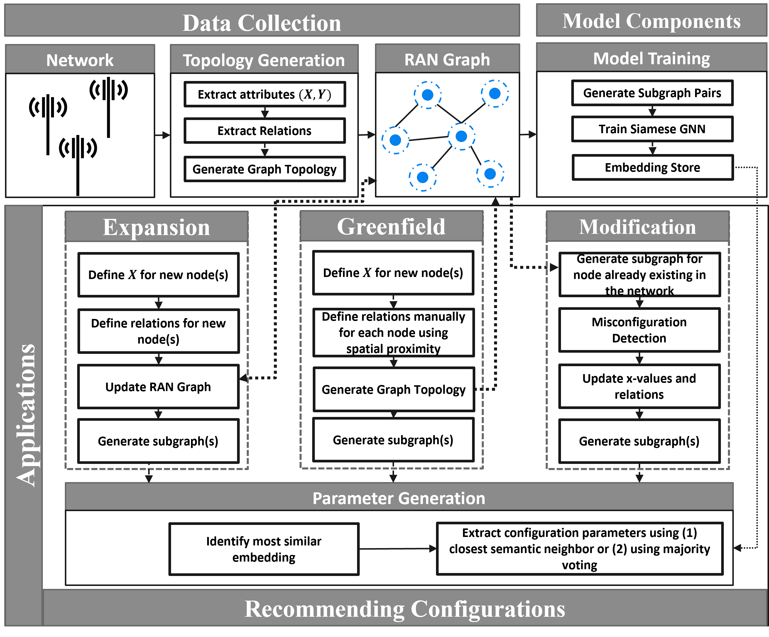
The configuration process in RAN is complex, often involving vendor default settings and additional adjustments based on deployment scenarios. Deployment typically includes two stages: Node Provisioning and Post-integration, with the latter requiring reconfigurations to achieve KPI acceptance. To address these challenges, this paper introduces a Deep Generative GNN, which aims to learn optimal parameters from stable networks and recommend configurations for other network areas. The approach involves three stages:
-
•
Stage I: Graph-based representation of multi-dimensional RAN data.
-
•
Stage II: Creation of subgraphs using a graph-sampling method and training a Siamese Graph Neural Network (S-GNN) with data from stable networks.
-
•
Stage III: Recommendation of Configuration Values tailored for different scenarios:
-
–
Expansion: Installing new cells on existing Radio Nodes.
-
–
Greenfield Deployment: Setting up new Radio Nodes in regions without existing infrastructure.
-
–
Modification: Adjusting existing cells and Radio Nodes to correct misconfigurations.
-
–
The method aims to develop a machine-assisted method for recommending network configuration parameters, transferring knowledge from stable operational networks, and identifying telecom system misconfigurations.
The key contributions of this work include:
-
1.
Developing an efficient configuration system with minimal manual intervention.
-
2.
Representing multidimensional RAN data as vectors in an embedding space.
-
3.
Introducing a robust, generalizable one-shot learning solution [2] that automatically updates with new data.
The paper’s structure is as follows: Section II introduces the methodology, and Section III details the evaluation metrics. Section IV details the results. Finally, section V concludes the paper with future research directions.
II Methodology
This section details the model architectures and the method for generating configuration values. The approach involves three stages, as shown in Figure 1.
II-A Data Description
The data for this study is collected from multiple eNBs and gNBs. This section details how data was collected and processed.
II-A1 Feature Values and Pre-processing
For this end, each cell in the telecom network is represented by two feature vectors in the dataset:
- •
-
•
- Configuration values displaying network variation, encompassing LTE attributes [1] like pZeroNominalPusch (target power level received by the eNB per resource block) and preambleInitialReceivedTargetPower (initial preamble power value), and NR attributes such as endcUlNrLowQualThresh and rachPreambleRecTargetPower [1].
These vectors combine LTE and NR attributes, facilitating model generalization across different technology deployments (4G, 5G, mixed mode), where N and M denote the number of LTE and NR cells in the network, respectively, is defined:
The datasets are then preprocessed as described in the following steps:
-
•
normalize values in each set to the range [0,1]
-
•
Concatenate sets:
-
•
Impute missing values by concatenating with 0.
II-B RAN Graph
The RAN is modeled as an undirected graph with vertices , each representing a RAN cell, and edges defining cell and inter-Radio Node relations, where
Subgraphs are , with being a random uniform sample of neighbors from , the vertices connected to . This approach focuses on local neighborhoods for configuring Radio Nodes or cells.
II-C Datasets for inductive Graph Neural Networks
GNNs are a class of machine learning models designed for learning and reasoning over graph-structured data. Unlike transductive GNNs, inductive GNNs [3] can generalize to unseen nodes and graphs. They achieve this by leveraging shared weights and aggregating information from neighboring nodes to learn node representations. Each subgraph has an associated feature set which is defined as:
| (1) |
Also, is the vector containing configuration values for the center cell for which the subgraph is constructed around. The dataset is then defined as:
| (2) |
II-D Model Definition & Architecture
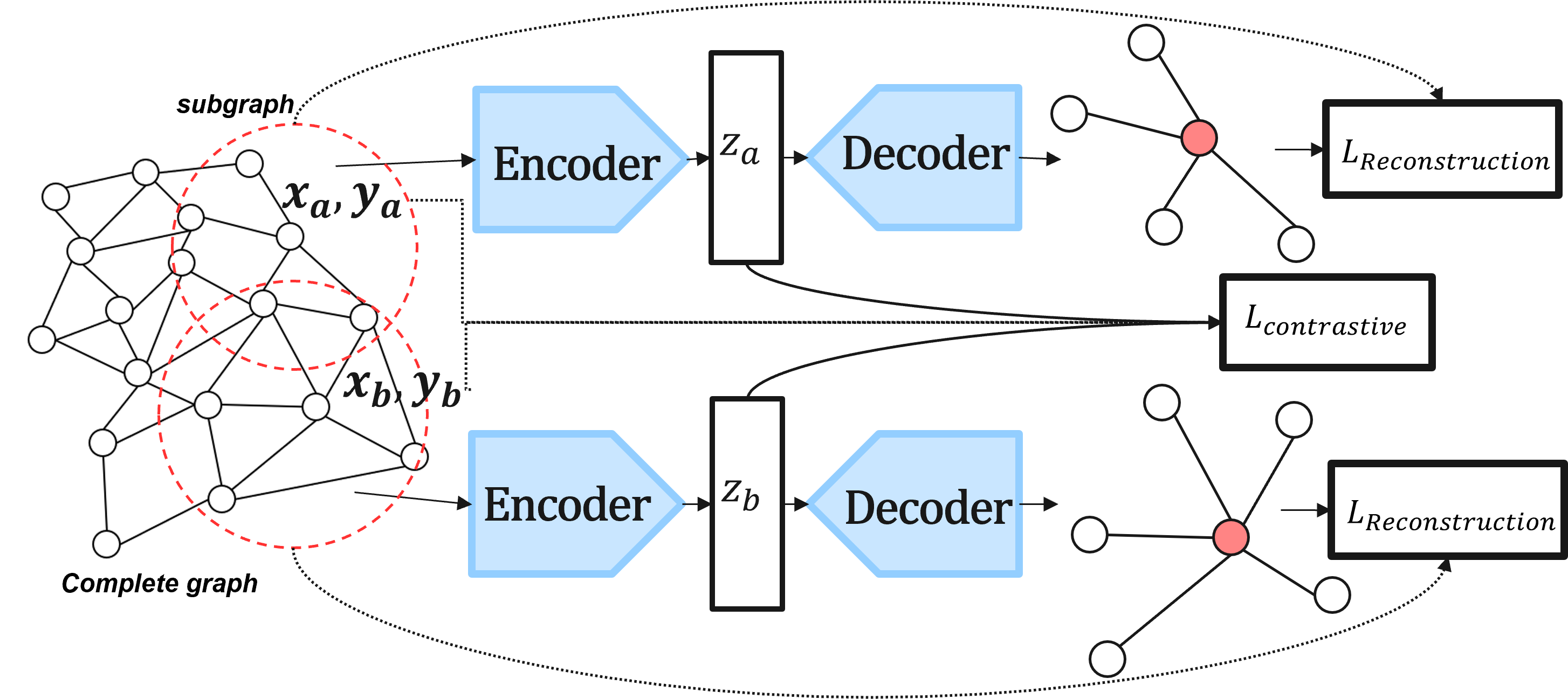
The models implemented in this study are one-shot meta-learners. The main model is an S-GNN-based model [4] that is trained using self-supervision through minimization of a contrastive loss. Figure 2 depicts the architecture of the model. The S-GNN is compared to a Graph Auto-Encoder (GAE) model that is trained through unsupervised learning.
The S-GNN and the GAE are functions represented by GNNs that are parameterized by and are defined as:
| (3) | |||
| (4) | |||
| (5) | |||
| (6) |
is the encoder part of the GAE and generates the latent space representation and reconstructs the input from the latent space. is the set of all embeddings of vertices associated with subgraph , where d is a hyperparameter that refers to the dimension of the latent space.
| (7) |
II-E Architecture & Training
The neural networks , , , each compose multi-headed Graph Attention (GATv2Conv) [5] and aggregates the output of each head using a Feed Forward Network (FFN).
The parameters in are trained with the objective to minimize the loss with as a hyperparameter:
| (8) |
| (9) |
are the labels, indicating how similar two arbitrary cells and are based on their corresponding configuration setups. Additionally, Subspace Learning is leveraged to limit the number of training pairs by identifying the most informative samples [6]. Informative pairs are composed of ambiguous samples, that is, samples that are close in the embedding space but belong to different classes.
The parameters in are trained with the objective to minimize the loss:
| (10) |
However, only will be used to infer the configuration values.
II-F Inference
The function that yields the configuration values for the cell that is introduced to the network after training is defined as:
| (11) |
where is either or , is the dataset that includes the N+M samples used for training and the samples that were introduced after the initial training.
| (12) |
Defines the set of all distances in the latent space from the new cell , to all other existing cells. The configuration values are generated using one of two methods.
II-F1 Using closest semantic subgraph neighbor
The configurations are acquired from the closest semantic subgraph in the embedding space.
| (13) |
II-F2 Using Majority voting
The configurations is acquired from an aggregation of the node’s closest neighbors in the latent space, where is a pre-defined parameter of neighbors.
| (14) |
is the smallest value in and is the set of loss values, excluding the set of losses:
This yields the configurations, as shown in equation (15).
| (15) |
where is an index value of the that yields which is the :th most optimal set of configuration values. Thus,
| (16) |
where aggregate is to be specified per attribute included in .
III Evaluation Metrics
This section details metrics used to evaluate the performance of the models.
III-A Configuration Accuracy Score
The accuracy of the generated configurations by the models across the whole network is then defined as:
| (17) |
Given are the configuration values for the cell network that yields the smallest with the embedding of cell .
III-B Misconfiguration Detection Score
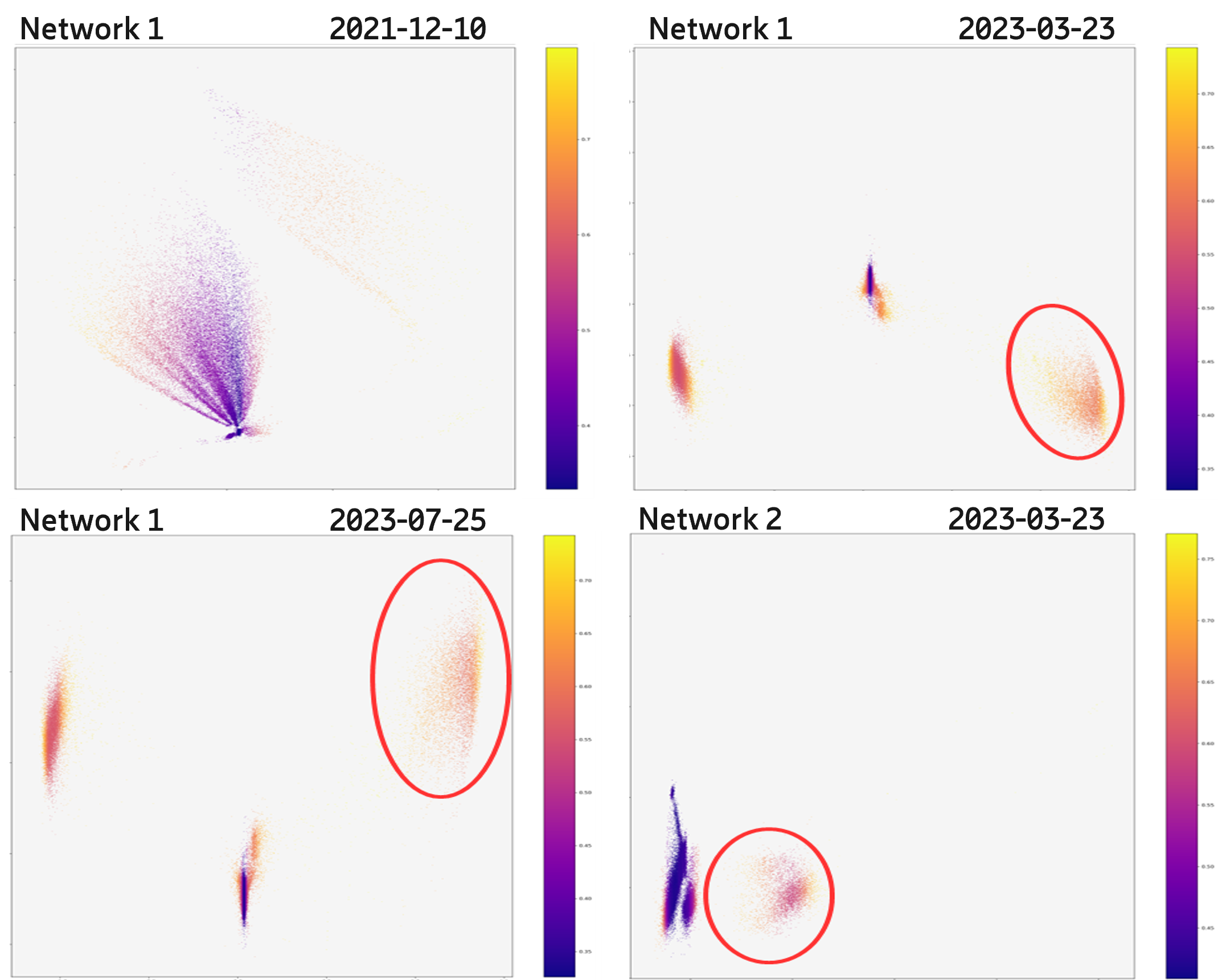
Anomaly detection is applied to evaluate the novelty of input samples in the network, providing operators with confidence values for the generated configurations. These values are anomaly scores, calculated by a model trained to identify novelties based on the distribution of embeddings in a latent space. If this score surpasses a predefined threshold, it signals the operator to reevaluate the specific instance.
| (18) |
Figure 4 presents the embeddings’ distributions with anomaly scores from iForest [7], indicating variation in network configurations.
IV Results
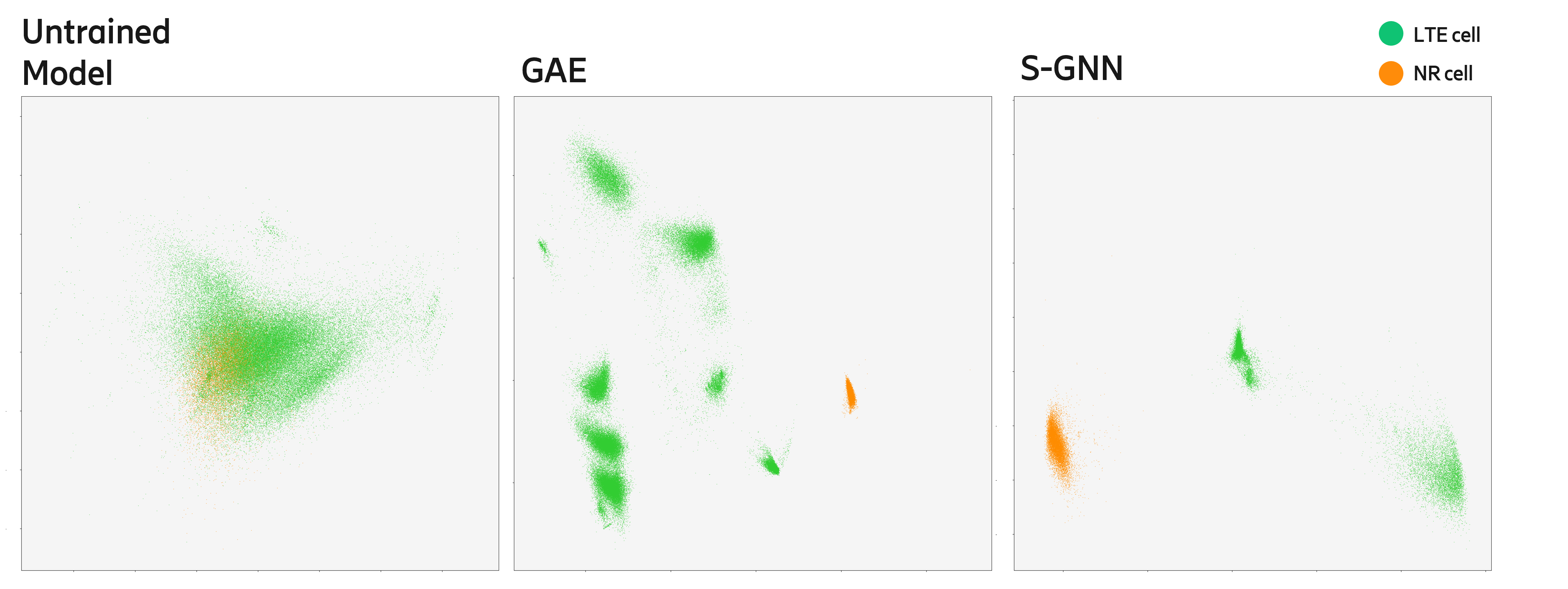
The paper evaluates two architectures, S-GNN and GAE, across four datasets. Their performance, measured using Average Optimal Cosine Similarity (17), is detailed in Table I. Higher scores in this measure correlate with better configuration prediction in telecom networks. Figure 3 illustrates the models’ 14-dimensional embeddings reduced to 2 dimensions via Principal Component Analysis (PCA), comparing an untrained model, GAE, and S-GNN. This visual representation highlights the distinct learning patterns of each model. GAE, an unsupervised model, demonstrates high accuracy in discerning different deployment contexts in the RAN, despite not being trained on configuration data. This indicates a strong correlation between the contextual information it processes and the resulting configurations.
In contrast, S-GNN shows higher accuracy in recognizing configuration setups when trained on both configuration and contextual data. However, this reliance on configuration data might lead to decreased adaptability over time as network settings evolve.
Figure 4 presents the embeddings’ distributions with anomaly scores. Notably, networks with less configuration variation show higher model accuracy, suggesting the models, especially S-GNN, perform better in more stable configuration environments. In summary, while GAE excels in unsupervised learning from non-configuration data, S-GNN is more accurate in supervised scenarios but may face challenges in adapting network configurations changes.
| Model | Dataset | Accuracy | ||
| Type | Network | Date | ||
| S-GNN | Test | 1 | 2021-12-10 | 0.888 |
| S-GNN | Train | 1 | 2023-03-23 | 0.953 |
| S-GNN | Test | 1 | 2023-07-25 | 0.921 |
| S-GNN | Test | 2 | 2023-03-23 | 0.990 |
| GAE | Test | 1 | 2021-12-10 | 0.906 |
| GAE | Train | 1 | 2023-03-23 | 0.916 |
| GAE | Test | 1 | 2023-07-25 | 0.907 |
| GAE | Test | 2 | 2023-03-23 | 0.991 |
V Conclusion and Future Direction
In this paper, the proposed framework enables mobile operators to generate a multitude of values for configuration parameters in telecom networks. At the core of this framework, a Deep Generative Model combines GNN and Siamese Neural Network. The framework represents RAN as a graph and then leverages subgraphs to enable inductive inference. The model generates embeddings which are used to infer configurations and to detect misconfiguration in the network. The model was evaluated on multiple datasets from operational networks. The model yields high accuracy on the datasets, indicating that the framework is generalizable and robust against concept drift.
In future developments, this work will focus on challenges related to recommending configurations for O-RAN [8] networks. Additionally, future work will involve eXplainable Artificial Intelligence (XAI) to demystify AI decisions, enhancing trust and transparency between machines and users.
References
- [1] 3GPP, “3gpp ts 32.300: Telecommunication management; configuration management (cm); name convention for managed objects,” 2024.
- [2] L. Bertinetto, J. F. Henriques, J. Valmadre, P. Torr, and A. Vedaldi, “Learning feed-forward one-shot learners,” Advances in neural information processing systems, vol. 29, 2016.
- [3] L. Anghinoni, Y.-t. Zhu, D. Ji, and L. Zhao, “Transgnn: A transductive graph neural network with graph dynamic embedding,” in 2023 International Joint Conference on Neural Networks (IJCNN), pp. 1–8, IEEE, 2023.
- [4] N. Mehrotra, N. Agarwal, P. Gupta, S. Anand, D. Lo, and R. Purandare, “Modeling functional similarity in source code with graph-based siamese networks,” IEEE Transactions on Software Engineering, vol. 48, no. 10, pp. 3771–3789, 2021.
- [5] S. Brody, U. Alon, and E. Yahav, “How attentive are graph attention networks?,” arXiv preprint arXiv:2105.14491, 2021.
- [6] E. Krivosheev, M. Atzeni, K. Mirylenka, P. Scotton, and F. Casati, “Siamese graph neural networks for data integration,” arXiv preprint arXiv:2001.06543, 2020.
- [7] X. Zhao, Y. Wu, D. L. Lee, and W. Cui, “iforest: Interpreting random forests via visual analytics,” IEEE transactions on visualization and computer graphics, 2018.
- [8] M. Polese, L. Bonati, S. D’oro, S. Basagni, and T. Melodia, “Understanding o-ran: Architecture, interfaces, algorithms, security, and research challenges,” IEEE Communications Surveys & Tutorials, 2023.